Inferring community structure in attributed hypergraphs using stochastic block models

Abstract

Hypergraphs are a representation of complex systems involving interactions among more than two entities and allow to investigation of higher-order structure and dynamics in real-world complex systems. Community structure is a common property observed in empirical networks in various domains. Stochastic block models have been employed to investigate community structure in networks. Node attribute data, often accompanying network data, has been found to potentially enhance the learning of community structure in dyadic networks. In this study, we develop a statistical framework that incorporates node attribute data into the learning of community structure in a hypergraph, employing a stochastic block model. We demonstrate that our model, which we refer to as HyperNEO, enhances the learning of community structure in synthetic and empirical hypergraphs when node attributes are sufficiently associated with the communities. Furthermore, we found that applying a dimensionality reduction method, UMAP, to the learned representations obtained using stochastic block models, including our model, maps nodes into a two-dimensional vector space while largely preserving community structure in empirical hypergraphs. We expect that our framework will broaden the investigation and understanding of higher-order community structure in real-world complex systems.

This work has been submitted to the IEEE for possible publication. Copyright may be transferred without notice, after which this version may no longer be accessible.

1 Introduction

A complex system is often represented as a network composed of nodes and pairwise interactions between the nodes. Various mathematical and computational methods have been developed to investigate the structure and dynamics of networks [20, 8, 44, 57]. Conventional modeling using dyadic networks (i.e., conventional networks, in which each edge connects a pair of nodes), however, may not accurately encode higher-order interactions among nodes (i.e., interactions among three or more nodes). In fact, higher-order interactions among nodes are not uncommon in real-world complex systems. Examples include group conversations in social contact networks [69, 51], co-authoring in collaboration networks [56, 62], joint purchase of products in co-purchasing networks [5], and many more [10]. Such complex systems can be represented as hypergraphs composed of nodes and hyperedges, where a hyperedge represents interaction among two or more nodes. In recent years, there has been notable progress in the development of measurements, dynamical process models, and theories for hypergraphs [71, 17, 11, 50, 18, 19]. This progress has uncovered that higher-order interactions among nodes are associated with structural properties, phenomena, and collective behaviors that cannot be adequately described by pairwise interactions alone (e.g., [4, 48, 55, 67]).

Community detection is a fundamental task that aims to describe the structure of a network by dividing the nodes into communities (i.e., sets of nodes such that each set of nodes is densely inter-connected) [59, 31, 32]. Numerous approaches for this task have been developed for dyadic networks [30, 31]. These methods have been extended to the case of hypergraphs [80, 42, 22, 21, 29, 23, 49, 79, 25, 66]. While communities are usually defined as disjoint sets of nodes, overlapping communities reflect that each node may belong to multiple communities in practice [60]. For example, an individual may belong to multiple communities via heterogeneous interactions with colleagues, friends, and neighbors in social networks [3].

A stochastic block model is a generative model for random graphs that assumes multiple communities underlying the network and latent parameters controlling intra- and inter-community interactions between nodes [38]. Stochastic block models have been deployed for investigating community structure in empirical networks [40, 43, 2, 45]. On one hand, basic models assume non-overlapping communities in a network. Previous studies have extended these models for dyadic networks to the case of hypergraphs [42, 22, 41, 23]. On the other hand, mixed-membership stochastic block models assume overlapping communities in a network [3]. Recent studies extended these models for dyadic networks to the case of hypergraphs [25, 66]. In this study, we focus on mixed-membership stochastic block models for hypergraphs.

Empirical network data is accompanied by node attribute data in many real-world complex systems. Examples of node attributes include the age, ethnicity, and gender of individuals in social networks [58, 26], affiliations of authors in collaboration networks [61, 54], and categories to which products belong in co-purchasing networks [5]. While node attributes do not always align with communities in a network [63], node attribute data potentially enhances the learning of community structure in dyadic networks [77, 58, 39, 75, 46, 26, 24, 9]. These previous studies motivate us to explore computational methods for incorporating node attribute data into the learning of community structure in hypergraphs.

In this study, we propose a mixed-membership stochastic block model for hypergraphs with node attributes. We refer to the proposed model as HyperNEO. The proposed model extends the Hy-MMSBM [66] and the MTCOV [26], which are both mixed-membership stochastic block models for networks, to the case of hypergraphs with node attributes. We demonstrate the capability of the proposed model in the learning of community structure in synthetic and empirical hypergraphs. Our code for the HyperNEO is available at https://github.com/kazuibasou/hyperneo.

2 Methods

2.1 Hypergraph with node attributes

A hypergraph consists of a set of nodes $V=\{v_{1},\ldots,v_{N}\}$ and a set of hyperedges $E$, where $N$ is the number of nodes. Any hyperedge $e$ is a subset of $V$ and its size $|e|$ is two or larger. We denote by $D$ the maximum size of the hyperedge in the hypergraph and $\Omega$ the set of all subsets of $V$ that have size of two or larger, including $V$ itself. We represent the hypergraph by an adjacency vector $\mathcal{A}=(A_{e})_{e\in\Omega}$, where $A_{e}$ represents the weight of hyperedge $e\in\Omega$. We assume that $A_{e}$ is a non-negative and discrete value for any $e\in\Omega$. In addition, each node $v_{i}$ belong to one of the $Z$ categories, as represented by a $Z$-dimensional attribute vector $(x_{iz})_{1\leq z\leq Z}$, where $x_{iz}=1$ if node $v_{i}$ belong to the $z$-th category and $x_{iz}=0$ otherwise for any $z\in\{1,\ldots,Z\}$. It holds true that $\sum_{z=1}^{Z}x_{iz}=1$ for any $i=1,\ldots,N$. We represent the attribute vectors for all the nodes as a $N\times Z$ matrix, denoted by $\bm{X}=(x_{iz})_{1\leq i\leq N,\ 1\leq z\leq Z}$.

2.2 Mixed-membership stochastic block model for hypergraphs with node attributes – HyperNEO

In this section, we propose a mixed-membership stochastic block model for hypergraphs with node attributes, which we refer to as HyperNEO. A mixed-membership stochastic block model (MMSBM) is a generative model for random graphs that allows each node to belong to multiple communities [3]. MMSBMs have been deployed for the learning of community structure in dyadic networks [7, 77, 27, 26]. These models have been extended to the case of hypergraphs [25, 66]. Hy-MMSBM is an MMSBM for hypergraphs without node attributes and exhibits a high performance on empirical hypergraphs in terms of inference accuracy and computation time [66]. MTCOV [26] is an MMSBM for multilayer dyadic networks (i.e., dyadic networks with multiple layers composed of sets of different types of interactions between nodes) with node attributes. We extend the Hy-MMSBM and the MTCOV to incorporate node attribute data into the learning of community structure in hypergraphs.

Our model is not the first to extend Hy-MMSBM and MTCOV to the case of hypergraphs with node attributes. In fact, HyCoSBM is an extension of these two models to the case of hypergraphs with node attributes [6]. Our model, however, does not impose any constraints on community memberships of the nodes in a hypergraph in inferring them, in contrast to the HyCoSBM. We find that our model achieves a comparable or higher quality of inferred communities in synthetic and empirical hypergraphs compared to the HyCoSBM (see Section 3 for numerical evidence).

2.2.1 Model

We model a hypergraph and node attributes probabilistically, assuming an underlying $K$ overlapping communities. Each node $v_{i}$ may belong to multiple communities. The propensity of $v_{i}$ belonging to each community is specified by a $K$-dimensional membership vector $(u_{ik})_{1\leq k\leq K}$, where $u_{ik}$ is a non-negative value for any $i=1,\ldots,N$ and any $k=1,\ldots,K$. We represent the membership vectors for all the nodes as a $N\times K$ matrix, denoted by $\bm{U}=(u_{ik})_{1\leq i\leq N,\ 1\leq k\leq K}$. The strength of intra- and inter-community interactions among nodes is represented by a symmetric $K\times K$ affinity matrix, denoted by $\bm{W}=(w_{kq})_{1\leq k\leq K,\ 1\leq q\leq K}$, where $w_{kq}$ is a non-negative value for any $k=1,\ldots,K$ and any $q=1,\ldots,K$. In addition, the strength of the association between each community and each category of the node attribute is represented by a $K\times Z$ matrix, denoted by $\bm{\beta}=(\beta_{kz})_{1\leq k\leq K,\ 1\leq z\leq Z}$, where $\beta_{kz}$ is a non-negative value for any $k=1,\ldots,K$ and any $z=1,\ldots,Z$. We assume $\sum_{z=1}^{Z}\beta_{kz}=1$ for any $k=1,\ldots,K$. We define the set of latent variables by $\bm{\theta}=(\bm{U},\bm{W},\bm{\beta})$. We assume the following as with MTCOV [26]: (i) $\mathcal{A}$ and $\bm{X}$ are conditionally independent given $\bm{\theta}$; (ii) $\bm{U}$ and $\bm{W}$ probabilistically generate $\mathcal{A}$, whereas $\bm{U}$ and $\bm{\beta}$ probabilistically generate $\bm{X}$.

We first model the network data $\mathcal{A}$ given $\bm{U}$ and $\bm{W}$. As with the Hy-MMSBM [66], we assume that the weight of hyperedge $e$ follows the Poisson distribution given by

$$P(A_{e}\ |\ \bm{U},\bm{W}) =e^{-\left(\frac{\lambda_{e}}{\kappa_{|e|}}\right)}\frac{\left(\frac{\lambda_{e}}{\kappa_{|e|}}\right)^{A_{e}}}{A_{e}!},$$ (1)

where

$$\lambda_{e} =\frac{1}{2}\sum_{v_{i}\in e}\sum_{v_{j}\in e\backslash\{v_{i}\}}\sum_{k=1}^{K}\sum_{q=1}^{K}u_{ik}u_{jq}w_{kq},$$ (2)

$$\kappa_{s} =\frac{s(s-1)}{2}\binom{N-2}{s-2}.$$ (3)

We also assume that the weights of the hyperedges in $\Omega$ are conditionally independent given $\bm{U}$ and $\bm{W}$ [66]:

$$P(\mathcal{A}\ |\ \bm{U},\bm{W})=\prod_{e\in\Omega}P(A_{e}\ |\ \bm{U},\bm{W}).$$ (4)

Then, the log-likelihood of $\mathcal{A}$ is given by [66]

$$\mathcal{L}_{\mathcal{A}}(\bm{U},\bm{W})=\sum_{e\in E}A_{e}\log(2\lambda_{e})-\frac{C}{2}\sum_{i=1}^{N}\sum_{j=1,\ j\neq i}^{N}\sum_{k=1}^{K}\sum_{q=1}^{K}u_{ik}u_{jq}w_{kq},$$ (5)

where

$$C=\sum_{s=2}^{D}\frac{1}{\kappa_{s}}\binom{N-2}{s-2}$$ (6)

and we discarded the terms not depending on $\bm{U}$ and $\bm{W}$.

We next model the node attribute data $\bm{X}$ given $\bm{U}$ and $\bm{\beta}$. Similar to the MTCOV [26], we assume that the attribute of node $v_{i}$ follow the multinomial distribution given by

$$P(x_{i1},\ldots,x_{iZ}\ |\ \bm{U},\bm{\beta})=\pi_{i1}^{x_{i1}}\dots\pi_{iZ}^{x_{iZ}},$$ (7)

where

$$\pi_{iz}=\frac{\sum_{k=1}^{K}u_{ik}\beta_{kz}}{\sum_{k^{\prime}=1}^{K}u_{ik^{\prime}}}$$ (8)

and it holds true that $\sum_{z=1}^{Z}\pi_{iz}=1$ for any $i=1,\ldots,N$ since we assume $\sum_{z=1}^{Z}\beta_{kz}=1$ for any $k=1,\ldots,K$. We also assume that the attributes of the nodes are conditionally independent given $\bm{U}$ and $\bm{\beta}$ [26]:

$$P(\bm{X}\ |\ \bm{U},\bm{\beta})=\prod_{i=1}^{N}P(x_{i1},\ldots,x_{iZ}\ |\ \bm{U},\bm{\beta}).$$ (9)

Then, the log-likelihood of $\bm{X}$ is given by

$$\mathcal{L}_{\bm{X}}(\bm{U},\bm{\beta})=\sum_{i=1}^{N}\sum_{z=1}^{Z}x_{iz}\log\left(\frac{\sum_{k=1}^{K}u_{ik}\beta_{kz}}{\sum_{k^{\prime}=1}^{K}u_{ik^{\prime}}}\right),$$ (10)

where we discarded the terms not depending on $\bm{U}$ and $\bm{W}$.

2.2.2 Inference

We turn to fit the latent parameters $\bm{\theta}$ to data $\mathcal{A}$ and $\bm{X}$. To this end, we deploy a maximum likelihood approach. Since we assume that $\mathcal{A}$ and $\bm{X}$ are conditionally independent given $\bm{\theta}$, the total log-likelihood, denoted by $\mathcal{L}(\bm{U},\bm{W},\bm{\beta})$, is decomposed into the sum of structural and attribute terms, i.e., $\mathcal{L}_{\mathcal{A}}(\bm{U},\bm{W})$ and $\mathcal{L}_{\bm{X}}(\bm{U},\bm{\beta})$. In practice, introducing a parameter $\gamma\in[0,1)$ that controls the relative contributions of the structural and attribute terms is useful for the learning of community structure in networks [77, 26]. Thus, we define the total log-likelihood as

$$\mathcal{L}(\bm{U},\bm{W},\bm{\beta})=(1-\gamma)\mathcal{L}_{\mathcal{A}}(\bm{U},\bm{W})+\gamma\mathcal{L}_{\bm{X}}(\bm{U},\bm{\beta}).$$ (11)

While one may fix $\gamma$ a priori, one may treat $\gamma$ as a hyperparameter [77, 26]. The inference procedure in our model with $\gamma=0$ is equivalent to that in the Hy-MMSBM [66]. Therefore, we describe the inference procedure in our model with $\gamma\in(0,1)$ in the following.

We aim to find $\bm{\theta}$ that maximizes Eq. (11). Since it is difficult to solve Eq. (11) analytically, we make it tractable using an expectation-maximization (EM) algorithm [28]. This approach has been used for inferring community structure in hypergraphs [25, 66]. First, using Jensen’s inequality gives the lower bound of $\mathcal{L}_{\mathcal{A}}(\bm{U},\bm{W})$ [66]:

$$\mathcal{L}_{\mathcal{A}}(\bm{U},\bm{W})\geq \mathcal{L}_{\mathcal{A}}(\bm{U},\bm{W},\rho)$$

$$= \sum_{e\in E}A_{e}\sum_{v_{i}\in e}\sum_{v_{j}\in e\backslash\{v_{i}\}}\sum_{k=1}^{K}\sum_{q=1}^{K}\rho_{ijkq}^{(e)}\log\left(\frac{u_{ik}u_{jq}w_{kq}}{\rho_{ijkq}^{(e)}}\right)-\frac{C}{2}\sum_{i=1}^{N}\sum_{j=1,\ j\neq i}^{N}\sum_{k=1}^{K}\sum_{q=1}^{K}u_{ik}u_{jq}w_{kq},$$ (12)

where $\rho_{ijkq}^{(e)}$ is a probability distribution that satisfies the condition $\sum_{v_{i}\in e}\sum_{v_{j}\in e\backslash\{v_{i}\}}\sum_{k=1}^{K}\sum_{q=1}^{K}\rho_{ijkq}^{(e)}=1$ [66]. The lower bound holds true when we take [66]

$$\rho_{ijkq}^{(e)}=\frac{u_{ik}u_{jq}w_{kq}}{2\lambda_{e}}.$$ (13)

Similarly, we apply Jensen’s inequality to $\mathcal{L}_{\bm{X}}(\bm{U},\bm{\beta})$:

$$\mathcal{L}_{\bm{X}}(\bm{U},\bm{\beta}) =\sum_{i=1}^{N}\sum_{z=1}^{Z}x_{iz}\log\left(\sum_{k=1}^{K}\frac{h^{\prime}_{izk}}{\sum_{k^{\prime}=1}^{K}u_{ik^{\prime}}}\frac{u_{ik}\beta_{kz}}{h^{\prime}_{izk}}\right)$$

$$=\sum_{i=1}^{N}\sum_{z=1}^{Z}x_{iz}\log\left(\sum_{k=1}^{K}h_{izk}\frac{u_{ik}\beta_{kz}}{h^{\prime}_{izk}}\right)$$

$$\geq\mathcal{L}_{\bm{X}}(\bm{U},\bm{\beta},h^{\prime},h)$$

$$=\sum_{i=1}^{N}\sum_{z=1}^{Z}x_{iz}\sum_{k=1}^{K}h_{izk}\log\left(\frac{u_{ik}\beta_{kz}}{h^{\prime}_{izk}}\right),$$ (14)

where $h^{\prime}_{izk}$ is a variable that satisfies the condition $\sum_{k=1}^{K}h^{\prime}_{izk}=\sum_{k^{\prime}=1}^{K}u_{ik^{\prime}}$, and $h_{izk}=h^{\prime}_{izk}/(\sum_{k^{\prime}=1}^{K}u_{ik^{\prime}})$ is a probability distribution that satisfies the condition $\sum_{k=1}^{K}h_{izk}=1$. The lower bound holds true when we take

$$h^{\prime}_{izk}=\frac{u_{ik}\beta_{kz}\sum_{k^{\prime}=1}^{K}u_{ik^{\prime}}}{\sum_{k^{\prime\prime}=1}^{K}u_{ik^{\prime\prime}}\beta_{k^{\prime\prime}z}}$$ (15)

and

$$h_{izk}=\frac{u_{ik}\beta_{kz}}{\sum_{k^{\prime\prime}=1}^{K}u_{ik^{\prime\prime}}\beta_{k^{\prime\prime}z}}.$$ (16)

The MTCOV [26] imposes the constraint that $\sum_{k^{\prime}=1}^{K}u_{ik^{\prime}}=1$ for any $i=1,\ldots,N$ to facilitate the partial differentiation of a lower bound of $\mathcal{L}_{\bm{X}}(\bm{U},\bm{\beta})$ with respect to $u_{ik}$. For the same purpose, the HyCoSBM [6] imposes the constraint that $0\leq u_{ik}\leq 1$ for any $i=1,\ldots,N$ and any $k=1,\ldots,K$. In contrast, instead of imposing a constraint on the membership matrix, we introduce the variable $h^{\prime}_{izk}$ to facilitate the partial differentiation of a lower bound of $\mathcal{L}_{\bm{X}}(\bm{U},\bm{\beta})$ with respect to $u_{ik}$. Note that $h_{izk}$ need to satisfy the condition $\sum_{k=1}^{K}h_{izk}=1$ to apply Jensen’s inequality to $\mathcal{L}_{\bm{X}}(\bm{U},\bm{\beta})$, whereas $h^{\prime}_{izk}$ is discarded when we perform partial differentiation of $\mathcal{L}_{\bm{X}}(\bm{U},\bm{\beta},h^{\prime},h)$ with respect to $u_{ik}$.

Overall, maximizing Eq. (11) is equivalent to maximizing

$$\mathcal{L}(\bm{U},\bm{W},\bm{\beta},\rho,h^{\prime},h)=(1-\gamma)\mathcal{L}_{\mathcal{A}}(\bm{U},\bm{W},\rho)+\gamma\mathcal{L}_{\bm{X}}(\bm{U},\bm{\beta},h^{\prime},h).$$ (17)

We maximize $\mathcal{L}(\bm{U},\bm{W},\bm{\beta},\rho,h^{\prime},h)$ by repeatedly updating $h^{\prime}$, $h$, $\rho$, and $\bm{\theta}$. We add Lagrange multiplier $\lambda^{(\bm{\beta})}=(\lambda_{1}^{(\bm{\beta})},\ldots,\lambda_{K}^{(\bm{\beta})})$ to enforce the constraint $\sum_{z=1}^{Z}\beta_{kz}=1$ for any $k=1,\ldots,K$:

$$\mathcal{L}^{\prime}(\bm{U},\bm{W},\bm{\beta},\rho,h^{\prime},h,\lambda^{(\bm{\beta})})=\mathcal{L}(\bm{U},\bm{W},\bm{\beta},\rho,h^{\prime},h)-\sum_{k=1}^{K}\lambda_{k}^{(\bm{\beta})}\left(\sum_{z=1}^{Z}\beta_{kz}-1\right).$$ (18)

We focus on updating $u_{ik}$. The partial derivative of $\mathcal{L}_{\mathcal{A}}(\bm{U},\bm{W},\rho)$ with respect to $u_{ik}$ is given by [66]

$$\frac{\partial}{\partial u_{ik}}\mathcal{L}_{\mathcal{A}}(\bm{U},\bm{W},\rho)=\frac{1}{u_{ik}}\left(\sum_{e\in E,\ v_{i}\in e}A_{e}\sum_{v_{j}\in e\backslash\{v_{i}\}}\sum_{q=1}^{K}\rho_{ijkq}^{(e)}\right)-\frac{C}{2}\sum_{j=1,\ j\neq i}^{N}\sum_{q=1}^{K}u_{jq}w_{kq}.$$ (19)

Then, the partial derivative of $\mathcal{L}_{\bm{X}}(\bm{U},\bm{\beta},h^{\prime},h)$ with respect to $u_{ik}$ is given by

$$\frac{\partial}{\partial u_{ik}}\mathcal{L}_{\bm{X}}(\bm{U},\bm{\beta},h^{\prime},h)=\frac{1}{u_{ik}}\sum_{z=1}^{Z}x_{iz}h_{izk}.$$ (20)

Setting the partial derivative of $\mathcal{L}^{\prime}(\bm{U},\bm{W},\bm{\beta},\rho,h^{\prime},h,\lambda^{(\bm{\beta})})$ with respect to $u_{ik}$ to zero yields

$$u_{ik}=\frac{2\left[(1-\gamma)\sum_{e\in E,\ v_{i}\in e}A_{e}\sum_{j=1,\ j\in e,\ j\neq i}^{N}\sum_{q=1}^{K}\rho_{ijkq}^{(e)}+\gamma\sum_{z=1}^{Z}x_{iz}h_{izk}\right]}{C(1-\gamma)\sum_{j=1,\ j\neq i}^{N}\sum_{q=1}^{K}u_{jq}w_{kq}}.$$ (21)

We focus on updating $w_{kq}$. It is sufficient to set the partial derivative of $\mathcal{L}_{\mathcal{A}}(\bm{U},\bm{W},\rho)$ with respect to $w_{kq}$ to zero, which has already done in Ref. [66]:

$$w_{kq}=\frac{2\sum_{e\in E}A_{e}\sum_{i=1,\ v_{i}\in e}^{N}\sum_{j=1,\ v_{j}\in e,\ j\neq i}^{N}\rho_{ijkq}^{(e)}}{C\sum_{i=1}^{N}\sum_{j=1,\ j\neq i}^{N}u_{ik}u_{jq}}.$$ (22)

We focus on updating $\beta_{kz}$. Setting the partial derivative of $\mathcal{L}^{\prime}(\bm{U},\bm{W},\bm{\beta},\rho,h^{\prime},h,\lambda^{(\bm{\beta})})$ regarding $\beta_{kz}$ to zero yields

$$\beta_{kz}=\frac{\sum_{i=1}^{N}x_{iz}h_{izk}}{\sum_{i^{\prime}=1}^{N}\sum_{z^{\prime}=1}^{Z}x_{i^{\prime}z^{\prime}}h_{i^{\prime}z^{\prime}k}}.$$ (23)

2.2.3 Implementation

The inference procedure in our model is as follows. We first initialize $\bm{\theta}=(\bm{U},\bm{W},\bm{\beta})$ uniformly at random. Then, we iterate $N_{\text{I}}$ times updating $\bm{U}$, $\bm{W}$, and $\bm{\beta}$ using Eqs. (21), (22), and (23), respectively. We set $N_{\text{I}}=20$ as in Ref. [58]. The computational complexity per iteration scales as $O(NKZ+|E|)$.

The EM algorithm is not guaranteed to converge to the global maximum [76]. To mitigate this issue, we adopt the same manner as Ref. [58]. First, we perform the above inference procedure independently $N_{\text{R}}$ times. Then, among the $N_{\text{R}}$ inferred results for $(\bm{U},\bm{W},\bm{\beta})$, we choose the one that yields the highest final value of $\mathcal{L}(\bm{U},\bm{W},\bm{\beta})$. We set $N_{\text{R}}=10$ as in Ref. [58]. We show the pseudocode of our algorithm in Supplementary Section S1.

2.2.4 Determining $K$ and $\gamma$

To deploy our model to a hypergraph with node attributes, we determine the values of the hyperparameters $K$ and $\gamma$. Unless we fix them a priori, we choose the pair of $K$ and $\gamma$ values such that our model achieves the highest accuracy in hyperedge prediction tasks among all candidate pairs of $K$ and $\gamma$ values [25, 66], as described below.

We perform a hyperedge prediction task as follows [25, 66]. Suppose that the train set of hyperedges, $E_{\text{train}}$, and the test set of hyperedges, $E_{\text{test}}$, are given. We use $E_{\text{train}}$ to infer the set of latent parameters $\bm{\theta}$. Then, we predict the hyperedges in $E_{\text{test}}$ using a set of inferred parameters. We use the area under the receiver-operator characteristic curve (AUC) as the accuracy metric for the prediction of the hyperedges in $E_{\text{test}}$. We compute the AUC as follows [25, 66]. First, for each hyperedge $e\in E_{\text{test}}$, we sample a hyperedge $e^{\prime}$ that satisfies the condition $|e|=|e^{\prime}|$ from the set $\Omega\ \backslash\ E_{\text{test}}$ uniformly at random without replacement. Let $R$ be the list of length $|E_{\text{test}}|$ of pairs $(e,e^{\prime})$ thus obtained. Then, we define the AUC as [25, 66]

$$\text{AUC}=\frac{1}{|R|}\left[\sum_{(e,\ e^{\prime})\in R}\bm{1}_{\{P(A_{e^{\prime}}\ >\ 0)\ >\ P(A_{e}\ >\ 0)\}}+0.5\sum_{(e,\ e^{\prime})\in R}\bm{1}_{\{P(A_{e^{\prime}}\ >\ 0)\ =\ P(A_{e}\ >\ 0)\}}\right],$$ (24)

where $\bm{1}_{\{\text{cond}\}}$ denotes an indicator function that returns 1 if the condition ‘cond’ holds true and returns 0 otherwise. We compute $P(A_{e}>0)$ for given hyperedge $e$ using Eq. (1) and the set of inferred parameters.

We compute the AUC for given $(K,\gamma)$ using the five-fold cross-validation. First, we partition the set $E$ into five subsets of equal size, denoted by $E_{1},\ldots,E_{5}$, uniformly at random. Then, we use the hyperedges in $E\ \backslash\ E_{i}$ as $E_{\text{train}}$ and use $E_{i}$ as $E_{\text{test}}$ to compute the AUC for each $i=1,\ldots,5$. The AUC for the $(K,\gamma)$ is the average of the five AUC values.

We choose $(K,\gamma)$ that yields the highest AUC among all the candidates for $(K,\gamma)$. Unless we state otherwise, we examine the $(Z-1)\times 9$ pairs of $K$ and $\gamma$, where $K\in\{2,3,\ldots,Z\}$ and $\gamma\in\{0.1,0.2,\ldots,0.9\}$.

2.3 Applying a dimensionality reduction method to the learned representation

To enhance the understanding of community structure, we map nodes into a two-dimensional vector space using inferred membership and affinity matrices. To this end, we first construct a $N\times N$ matrix, denoted by $\bar{\bm{A}}=(\bar{a}_{ij})_{1\leq i\leq N,\ 1\leq j\leq N}$. We define $\bar{a}_{ij}$ for each $i=1,\ldots,N$ and each $j=1,\ldots,N$ such that $i\neq j$ as the expectation conditional on Eq. (1) of the sum of the weights over the hyperedges to which nodes $v_{i}$ and $v_{j}$ belong:

$$\bar{a}_{ij}=\sum_{e\in E,\ v_{i}\in e,\ v_{j}\in e}\frac{\lambda_{e}}{\kappa_{|e|}},$$ (25)

where we calculate $\lambda_{e}$ for given hyperedge $e$ using the inferred membership and affinity matrices. We define $\bar{a}_{ii}=0$ for any $i=1,\ldots,N$. Note that $\bar{a}_{ij}=0$ for $i\neq j$ if and only if nodes $v_{i}$ and $v_{j}$ do not share any hyperedge in $E$. Then, we apply a topology-based dimensionality reduction method (UMAP [52]) to the learned representation $\bar{\bm{A}}$ to obtain a two-dimensional representation of each node. To this end, we used the ‘UMAP’ function in the ‘umap-learn’ library [1]. The UMAP has been deployed for the dimensionality reduction and clustering of high-dimensional data across disciplines [12, 53, 64, 16, 14].

The ‘UMAP’ function has three major hyperparameters that can have a significant impact on the resulting embedding in addition to the dimensionality of the reduced space (i.e., ‘n_components’; we set ‘n_components’ as two) [1]: (i) ‘n_neighbors’, balancing local and global structure in the input data; (ii) ‘min_dist’, controlling how tightly the UMAP is allowed to pack data points together in the reduced space; and (iii) ‘metric’, controlling how distance is computed in the ambient space of the input data. We set ‘n_neighbors’ as the average degree of the node in a given hypergraph, where we define the degree of a node as the number of hyperedges to which the node belongs. We set ‘min_dist’ as 0.1 as default. We examine two distance metrics: Euclidean distance (specified by setting ‘metric’ as ‘euclidean’) and the cosine distance (specified by setting ‘metric’ as ‘cosine’).

3 Results

3.1 Synthetic hypergraphs

We begin by assessing the proposed model on synthetic hypergraphs. We fix 1,000 nodes, two communities, and two categories of the node attribute. The set of parameters $\{p_{\bm{U}},w_{\text{in}},D,|E|/N\}$ control community structure and node attributes in our synthetic hypergraphs (see Supplementary Section S2 for details). For a given combination of parameter values $(p_{\bm{U}},w_{\text{in}},D,|E|/N)$, we independently generate 100 hypergraphs using the algorithm proposed in Ref. [65]. Then, we compute the average of the cosine similarity between the ground-truth membership matrix and an inferred membership matrix of the proposed model over the 100 hypergraphs (see Supplementary Section S3 for the definition of the cosine similarity). We set the hyperparameter $K=2$ in the proposed model.

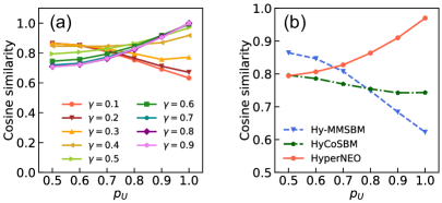
Figure 1: Inference accuracy of the proposed model when we vary the strength of the association between the communities and node attributes in synthetic hypergraphs. (a) Cosine similarity for the proposed model with a given value of $\gamma$. (b)–(f) Comparison of the cosine similarity between the proposed model and the two baseline models.

Figure 1(a) shows the cosine similarity for the proposed model with a given value of the hyperparameter $\gamma$ when we vary the parameter $p_{\bm{U}}$ for synthetic hypergraphs. The hyperparameter $\gamma$ controls the extent to which the proposed model incorporates node attribute data into the learning of community structure in a given hypergraph. In our synthetic hypergraphs, the propensity to which a node belongs to different communities is controlled by $p_{\bm{U}}$ and the attribute of a node explicitly encodes the propensity of the node (see Supplementary Section S2 for details). Therefore, the value of $\gamma$ at which the proposed model achieves the highest cosine similarity is expected to depend on $p_{\bm{U}}$. Indeed, when $p_{\bm{U}}=0.5$, the proposed model with a smaller value of $\gamma$ yields a higher cosine similarity (see Fig. 1(a)), indicating that the node attributes little contribute to the learning of the community structure. This is because each node belongs to the two communities with the same propensity when $p_{\bm{U}}=0.5$, making it difficult to associate the node attributes with the communities. On the other hand, when $p_{\bm{U}}=1.0$, the proposed model with a higher value of $\gamma$ yields a higher cosine similarity (see Fig. 1(a)). This is because each node belongs to one of the two communities when $p_{\bm{U}}=1.0$, and the community to which each node belongs is directly linked with the attribute of the node.

We next compare the proposed model with the two baseline models (i.e., Hy-MMSBM [66] and HyCoSBM [6]) in terms of the inference accuracy in synthetic hypergraphs. Hy-MMSBM uses only network data in the learning of community structure in a hypergraph. HyCoSBM is an MMSBM for hypergraphs with node attributes. In contrast to the proposed model, the HyCoSBM imposes a constraint on the membership matrix in inferring it. Unless we state otherwise, we set the same number of iterations for a set of initial parameters and the same number of sets of random initial parameters (i.e., $N_{\text{I}}=20$ and $N_{\text{R}}=10$, respectively) in all the models. We set the hyperparameter $K=2$ in all the models and set the hyperparameter $\gamma=0.5$ in the HyCoSBM and the proposed model. We compute the average of the cosine similarity for each model over the 100 hypergraphs generated for a given combination $(p_{\bm{U}},w_{\text{in}},D,|E|/N)$.

We found that the cosine similarity for the proposed model is higher than that for the Hy-MMSBM when $0.7\leq p_{\bm{U}}\leq 1.0$ and that for the HyCoSBM when $0.6\leq p_{\bm{U}}\leq 1.0$ (see Fig. 1(b)). We also found that the cosine similarity for the proposed model usually is higher than that for the two baseline models when we fix $p_{\bm{U}}=0.8$ and vary any one of the structural parameters (i.e., $w_{\text{in}}$, $D$, or $|E|/N$; see Supplementary Section S4 for details). We compare the inference accuracy between the proposed model and the HyCoSBM when we vary the value of $\gamma$ in Supplementary Section S5.

These results for synthetic hypergraphs indicate the following. First, node attribute data contributes to the learning of community structure in hypergraphs when node attributes are sufficiently associated with the communities. This extends previous results for dyadic networks [58, 26] and is consistent with those for hypergraphs [6]. Second, not imposing any constraint on the membership matrix in inferring it yields a comparable or higher inference accuracy than imposing it.

Table 1: AUC in hyperedge prediction tasks on the empirical hypergraphs. We show the mean $\pm$ standard deviation of the AUC across 100 independent runs for each model in each data set.

Data	Hy-MMSBM	HyCoSBM	HyperNEO	HyCoSBM	HyperNEO
				$\gamma=0.5$	$\gamma=0.5$
workplace	0.703 $\pm$ 0.016	0.755 $\pm$ 0.015	0.754 $\pm$ 0.015	0.707 $\pm$ 0.017	0.714 $\pm$ 0.016
hospital	0.769 $\pm$ 0.009	0.776 $\pm$ 0.008	0.771 $\pm$ 0.008	0.775 $\pm$ 0.008	0.769 $\pm$ 0.009
high-school	0.868 $\pm$ 0.006	0.905 $\pm$ 0.003	0.913 $\pm$ 0.003	0.888 $\pm$ 0.004	0.906 $\pm$ 0.003
primary-school	0.789 $\pm$ 0.006	0.834 $\pm$ 0.003	0.850 $\pm$ 0.003	0.802 $\pm$ 0.005	0.830 $\pm$ 0.004

3.2 Empirical hypergraphs

We turn to apply the proposed model to empirical hypergraphs with node attributes. See Supplementary Table S6 for the properties of the empirical hypergraphs. The ground-truth communities are not available for the empirical hypergraphs. In such cases, one performs a task that potentially measures the quality of inferred communities in a network, including link prediction tasks [36]. Therefore, we compare the proposed model with the two baseline models in terms of the AUC in hyperedge prediction tasks, as in Refs. [25, 66]. We examine the hyperparameter $K$ from 2 to $Z$ in increments of 1 in all the models; we examine the hyperparameter $\gamma$ from 0.1 to 0.9 in increments of 0.1 in the HyCoSBM and the proposed model. The procedure to compute the AUC for any model with a given hyperparameter set follows the same manner as described in Section 2.2.4 because all the models assume that the weight of a given hyperedge $e$ follows the same Poisson distribution given by Eq. (1). Hereafter, unless we state otherwise, we set the hyperparameter set that yields the highest mean of the AUC among all candidates in each model in each hypergraph (see Supplementary Table S7 for the hyperparameter sets).

Table 1 compares the AUC between the proposed model and the two baseline models in the empirical hypergraphs. First, the AUC for the proposed model is significantly higher than that for the Hy-MMSBM in each of the workplace, high-school, and primary-school hypergraphs (the $P$-value is less than 0.005 according to the Welch’s $t$-test) and is comparable in the hospital hypergraph. Second, the AUC for the proposed model is significantly higher than that for the HyCoSBM in each of the high-school and primary-school hypergraphs (the $P$-value is less than 0.005 according to the Welch’s $t$-test) and is comparable in other hypergraphs.

Tuning the value of $\gamma$ in the proposed model entails additional computational overhead compared to the Hy-MMSBM. In practical contexts, one may also set $\gamma=0.5$ in the proposed model, regardless of the strength of the association between the communities and node attributes in a given hypergraph. Therefore, we compute the AUC for the proposed model with $\gamma=0.5$ and the HyCoSBM with $\gamma=0.5$ while setting the same $K$ value in each model and each hypergraph (see Table 1). We found that the AUC for the proposed model with $\gamma=0.5$ is significantly higher than that for the Hy-MMSBM and that for the HyCoSBM with $\gamma=0.5$ in each of the workplace, high-school, and primary-school hypergraphs (the $P$-value is less than 0.005 according to the Welch’s $t$-test).

These results suggest that incorporating node attribute data into the learning of community structure contributes to the prediction of hyperedges in the workplace, high-school, and primary-school hypergraphs but little in the hospital hypergraph. In addition, inferred affinity matrices indicate that each empirical hypergraph has a community structure (i.e., nodes have more intra-community interactions than inter-community interactions; See Supplementary Section S8 for details). In the following, we further explore the association between community structure and node attributes in each empirical hypergraph using the three models. We present the results obtained by fixing a random seed in each empirical hypergraph.

3.2.1 Workplace

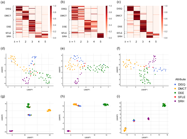
Figure 2: Inference of community structure in the workplace hypergraph. (a)–(c) Inferred membership matrices. (d)–(i) UMAP plots of the individuals. We use the Euclidean distance in (d)–(f) and the cosine distance in (g)–(i) in the UMAP. In this figure and Figs. 3–5, the results for the Hy-MMSBM are shown in (a), (d), and (g), those for the HyCoSBM are shown in (b), (e), and (h), and those for the proposed model are shown in (c), (f), and (i); in panels (a)–(c), we arrange the $N$ row indices according to the attributes of the nodes in each hypergraph.

We first focus on the workplace hypergraph composed of 92 individuals (i.e., nodes) working in an office building in France and 788 contact events (i.e., hyperedges) among them [35, 66]. The attribute of an individual is their department affiliation. Each individual belongs to one of the five departments: DISQ, DMCT, DSE, SFLE, and SRH.

Figures 2(a)–2(c) show inferred membership matrices of the three models (see Supplementary Section S8 for the visualization method). The result for Hy-MMSBM suggests that individuals in the DISQ, DMCT, DSE, and SRH departments tend to belong to distinct communities (see Fig. 2(a)). The result for HyCoSBM suggests that individuals in the DISQ, DMCT, and SFLE departments have similar community memberships and those in the DSE and SRH departments tend to belong to distinct communities (see Fig. 2(b)). The result for the proposed model more strongly suggests that individuals in the DISQ, DMCT, DSE, and SRH departments have distinct community memberships, compared to that for Hy-MMSBM (see Fig. 2(c)).

To further understand the association between community structure and the departments of individuals, we map the individuals into a two-dimensional vector space. We first compute the learned representation $\bar{\bm{A}}$ using the inferred membership and affinity matrices of a given model. Then, we apply a dimensionality reduction method (UMAP [52]) to the matrix $\bar{\bm{A}}$ to obtain a set of two-dimensional vectors of the individuals. We follow the same manner described in Section 2.3 for any model because all the models assume the same Poisson distribution, given by Eq. (1), regarding the weight of a given hyperedge $e$.

Figures 2(d)–2(f) show UMAP plots of the individuals for each model, where the two axes correspond to UMAP1 and UMAP2. We use the Euclidean distance as a distance metric in the UMAP. We found that individuals who have similar community memberships are positioned closely to each other for any model. In fact, for the Hy-MMSBM and the proposed model, individuals in the same department are positioned closely, and those in different departments are moderately far apart from each other (see Figs. 2(d) and 2(f)). For the HyCoSBM, individuals in the DISQ and DMCT are positioned closely to each other (see Fig. 2(e)).

Individuals who have similar community memberships but different numbers of contacts may be positioned far apart in the space when we use the Euclidean distance in the UMAP. Therefore, we next use the cosine distance in the UMAP to mitigate differences in the number of contacts between individuals. As expected, employing the cosine distance in the UMAP enables a more straightforward identification of individuals who have similar community memberships in the space, compared to using the Euclidean distance in the UMAP (see Figs. 2(g)–2(i)).

To sum up, we conclude that the workplace hypergraph has a community structure associated with the departments of individuals. These results are consistent with the previous results that individuals have more intra-departmental contacts than inter-departmental contacts [35]. We also found that applying the UMAP to the learned representation, $\bar{\bm{A}}$, maps the individuals into a two-dimensional vector space while largely preserving their community memberships.

3.2.2 Hospital

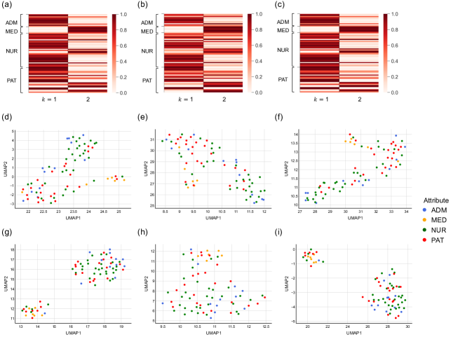
Figure 3: Inference of community structure in the hospital hypergraph. (a)–(c) Inferred membership matrices. (d)–(i) UMAP plots of the individuals. We use the Euclidean distance in (d)–(f) and the cosine distance in (g)–(i) in the UMAP.

We focus on the hospital hypergraph composed of 75 individuals (i.e., nodes) in a hospital and 1,825 contacts (i.e., hyperedges) among them [74, 66]. The attribute of an individual is the class to which they belong. Each individual belongs to one of the four classes according to their activity in the ward: patients (PAT), medical doctors (MED), paramedical staff (NUR), and administrative staff (ADM).

The three models produce qualitatively similar inferred membership matrices (see Figs. 3(a)–3(c)). They suggest that individuals in the same activity class do not strongly belong to the same community (see Figs. 3(a)–(c)). Figures 3(d)–3(f) show UMAP plots of the individuals for each model when we use the Euclidean distance in the UMAP. The individuals are relatively sparsely distributed over the space for any model. On the other hand, when we use the cosine distance in the UMAP, we find two sets of individuals who have similar community memberships for the Hy-MMSBM and the proposed model (see Figs. 3(g) and (i)); for example, the medical doctors are positioned closely to each other in one set (see Figs. 3(g) and (i)). The individuals are still sparsely distributed over the space for the HyCoSBM (see Fig. 3(h)).

These results suggest that there is not a strong association between the activity classes of individuals and the community structure in the hospital hypergraph. In fact, the original time series data contain a high frequency of contacts between medical doctors and between paramedical staff but fewer contacts between patients and between administrative staff [74]. The limited number of contacts between patients may be a characteristic of the wards with mostly single rooms in the hospital [74]. Such contact patterns due to some localization of individuals (e.g., patients in different rooms may have few contacts; patients and paramedical staff in different wards may have few contacts) have also been discussed in Ref. [72].

3.2.3 High school

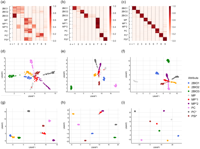
Figure 4: Inference of community structure in the high-school hypergraph. (a)–(c) Inferred membership matrices. (d)–(i) UMAP plots of the students. We use the Euclidean distance in (d)–(f) and the cosine distance in (g)–(i) in the UMAP.

We focus on the high-school hypergraph composed of 327 students (i.e., nodes) in a high school in France and 7,818 contact events (i.e., hyperedges) among them [51, 23, 15]. The attribute of a student is the class to which the student belongs. Each student belongs to one of the nine classes: three classes on mathematics and physics (MP, $\text{MP}^{*}$1, and $\text{MP}^{*}$2), three classes on biology (2BIO1, 2BIO2, and 2BIO3), two classes on physics and chemistry (PC and $\text{PC}^{*}$), and one class on engineering studies ($\text{PSI}^{*}$).

Figures 4(a)–4(c) show inferred membership matrices of the three models. The result for the Hy-MMSBM suggests that students in the biology classes have similar community memberships, as do those in the MP, $\text{MP}^{*}$1, PC, and $\text{PSI}^{*}$ classes (see Fig. 4(a)). The result for the HyCoSBM suggests that students in the mathematics and physics classes have similar community memberships and other students have different community memberships in different classes (see Fig. 4(b)). The result for the proposed model suggests that students have different community memberships in different classes (see Fig. 4(c)). These results are largely consistent with previous results that students have more intra-class contacts than inter-class contacts [51]. Figures 4(d)–4(f) plot the students in a two-dimensional vector space for each model when we use the Euclidean distance in the UMAP. We find that students who have similar community memberships are positioned closely to each other in the space for any model. In fact, students in the biology classes are positioned closely to each other for the Hy-MMSBM (see Figs. 4(d)); those in the mathematics and physics classes are positioned closely to each other for the HyCoSBM (see Figs. 4(e)); those in the same class are positioned closely to each other and those in different classes are moderately far apart from each other for the proposed model (see Figs. 4(f)). In addition, using the cosine distance in the UMAP allows us to more easily find students who have similar community memberships in the space, compared to using the Euclidean distance in the UMAP (Figs. 4(g)–4(i)). Therefore, we conclude that the high-school hypergraph has a community structure associated with the classes of students.

3.2.4 Primary school

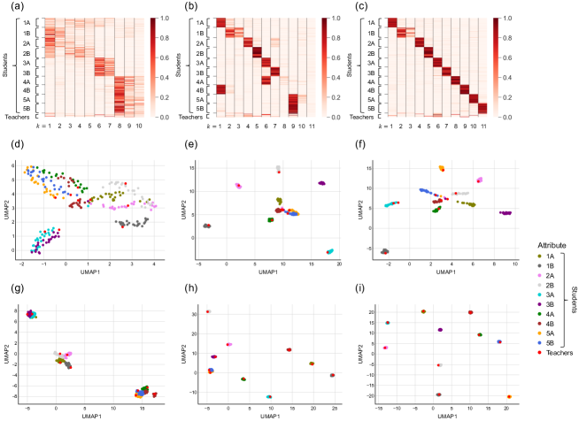
Figure 5: Inference of community structure in the primary-school hypergraph. (a)–(c) Inferred membership matrices. (d)–(i) UMAP plots of the individuals. We use the Euclidean distance in (d)–(f) and the cosine distance in (g)–(i) in the UMAP.

We finally focus on the primary-school hypergraph composed of 242 individuals (i.e., 232 students and 10 teachers; they are represented as nodes) in a primary school in France and 12,704 contact events (i.e., hyperedges) among them [69, 34, 23, 15]. The attribute of a student is the class to which they belong. There are two classes for each of the five grades: 1A, 1B, 2A, 2B, 3A, 3B, 4A, 4B, 5A, and 5B. Each student belongs to one of the ten classes. The teachers are grouped as a separate category.

Figures 5(a)–5(c) show inferred membership matrices of the three models. First, the result for any model suggests that teachers belong to different communities in a decentralized manner (see Figs. 5(a)–5(c)). These results are consistent with previous results that teachers do not have much more contact with each other than they do with students [69]. Second, the three models produce qualitatively different results for community memberships of students. The result for the Hy-MMSBM suggests that students in the first and second grades have similar community memberships, those in the third grade do, and those in the fourth and fifth grades do (see Fig. 5(a)). The result for the HyCoSBM suggests that students in the first, second, and third grades have different community memberships in different classes and those in the fifth grade have similar community memberships (see Fig. 5(b)). The result for the proposed model suggests that students have largely different community memberships in different classes (see Fig. 5(c)). These results are largely consistent with previous results that most contacts occur among students in the same class [69]. Figures 5(d)–5(f) show UMAP plots of the individuals for each model when we use the Euclidean distance in the UMAP. The set of embedded coordinates of the individuals is largely consistent with their community memberships for each model. In fact, teachers are dispersedly positioned in the space for any model (see Figs. 5(d)–5(f)). For the Hy-MMSBM, students in the first and second grades are positioned closely to each other, those in the third grade are, and those in the fourth and fifth grades are (see Fig. 5(d)). For the HyCoSBM, students in the fifth grade are positioned closely to each other (see Fig. 5(e)). For the proposed model, students in the same class are positioned closely to each other and those in different classes are moderately far apart from each other (see Fig. 5(f)). In addition, using the cosine distance in the UMAP makes it easier to find students who have similar community memberships in the space than using the Euclidean distance in the UMAP (see Figs. 5(g)–5(i)). Therefore, we conclude that the primary-school hypergraph has a community structure associated with the classes of students.

4 Discussion

We proposed a mixed membership stochastic block model for hypergraphs with node attributes called the HyperNEO. We compared the proposed model with Hy-MMSBM [66] and HyCoSBM [6] in terms of the capability of learning community structure in hypergraphs. Our results indicate that incorporating node attribute data enhances the learning of community structure in hypergraphs when node attributes are sufficiently correlated with the communities, which extends previous results for dyadic networks [77, 58, 39, 75, 46, 26, 9] and is consistent with the previous results for hypergraphs [6].

We extend the Hy-MMSBM [66] and the MTCOV [26] to incorporate node attribute data into the learning of community structure in a given hypergraph. The HyCoSBM [6] is an existing extension of these two models to the case of hypergraphs with node attributes. The proposed model includes a main significant addition to the HyCoSBM. Namely, the proposed model does not impose any constraint on the membership matrix in inferring it. Existing models similarly do not impose any constraint on the membership matrix [7, 27, 25, 66] (but see [77, 37, 78, 26, 6]). We found that the proposed model achieves comparable or higher fitting quality of community structure in synthetic and empirical hypergraphs compared to the HyCoSBM.

The proposed model introduces the hyperparameter $\gamma$, similar to the HyCoSBM [6]. The hyperparameter $\gamma$ controls the extent to which the model incorporates node attribute data into the learning of community structure in a hypergraph. We observed that the inference accuracy of the proposed model remarkably depends on the value of $\gamma$ and the strength of association between community structure and node attributes in synthetic hypergraphs. We tuned the value of $\gamma$ in empirical hypergraphs using cross-validation. In practical scenarios, one may also use the proposed model with $\gamma=0.5$ regardless of the strength of the association between community structure and node attributes in a given hypergraph. In fact, we found that the proposed model with $\gamma=0.5$ usually achieves a higher quality of fitting community structure than the HyCoSBM with $\gamma=0.5$ in synthetic and empirical hypergraphs.

We found the use of stochastic block models to map nodes into a two-dimensional vector space while largely preserving their community memberships in hypergraphs. In fact, we have demonstrated that node layouts obtained using the three models (i.e., Hy-MMSBM [66], HyCoSBM [6], and the proposed model) largely preserve inferred community memberships of the nodes in empirical hypergraphs. The development of standard tools to visualize a hypergraph is still ongoing [81, 47]. A basic method is to apply a force-directed algorithm [33] to the one-mode projected network of a given hypergraph [47]. For comparison, we show other node layouts [33, 68, 10] for empirical hypergraphs in Supplementary Section S9. We expect that the use of stochastic block models for the node layout facilitates the understanding of community structure in empirical hypergraphs.

We did not systematically examine different dimensionality reduction methods. We employed the UMAP, which has been used for the visualization and clustering of high-dimensional data across disciplines [12, 53, 64, 16, 14]. Other dimensionality reduction methods (e.g., Laplacian eigenmaps [13], Isomap [70], and t-SNE [73]) may yield qualitatively different results on community structure in the empirical hypergraphs used in our study. In addition, we focused on only the case of unordered attribute data (i.e., the index of the category to which a node belongs is not informative). It warrants future work to extend the proposed model to the case where the node attributes are ordered discrete values or continuous values [58, 68].

Supplementary Materials for:
Inferring community structure in attributed hypergraphs using stochastic block models

Kazuki Nakajima and Takeaki Uno

S1 Pseudocode of the HyperNEO

Algorithm S1 shows the pseudocode of our algorithm.

Algorithm S1 HyperNEO

0:  Hypergraph with node attributes: $(V,E,\bm{X})$, number of random initializations: $N_{\text{R}}$, number of iterations: $N_{\text{I}}$, and scaling parameter: $\gamma$.

0:  Inferred parameters: $(\bm{U},\bm{W},\bm{\beta})$.

1:  BestLoglik $=-\infty$

2:  BestParams $=$ None

3:  for $r=1,\ldots,N_{\text{R}}$ do

4:     Initialize $\bm{U}$, $\bm{W}$, and $\bm{\beta}$ uniformly at random.

5:     for $i=1,\ldots,N_{\text{I}}$ do

6:        Calculate $\rho$ using Eq. (13) and $h$ using Eq. (16).

7:        Update $\bm{U}$ using Eq. (21).

8:        Update $\bm{W}$ using Eq. (22).

9:        Update $\bm{\beta}$ using Eq. (23).

10:     L $\leftarrow(1-\gamma)\mathcal{L}_{\mathcal{A}}(\bm{U},\bm{W})+\gamma\mathcal{L}_{\bm{X}}(\bm{U},\bm{W})$

11:     if L $>$ BestLoglik then

12:        BestLoglik $\leftarrow$ L

13:        BestParams $\leftarrow(\bm{U},\bm{W},\bm{\beta})$

14:  return  BestParams

S2 Synthetic hypergraphs

As benchmark data, we generate hypergraphs with node attributes as follows. We fix $N=1,000$ nodes, $K=2$ communities, and $Z=2$ categories of the node attribute. We introduce the set of parameters $\{p_{\bm{U}},w_{\text{in}},D,|E|/N\}$ to control community structure and node attributes. First, we generate a hypergraph with community structure using the algorithm presented in Ref. [14]. To this end, we input $\bm{U}$, $\bm{W}$, and the distribution of the hyperedge size to the algorithm to sample a hypergraph conditioned on them as follows. We input $\bm{U}$ using a given probability $p_{\bm{U}}$: we assign the membership vector $[p_{\bm{U}},1-p_{\bm{U}}]$ to 500 nodes chosen uniformly at random and the membership vector $[1-p_{\bm{U}},p_{\bm{U}}]$ to other nodes. We input $\bm{W}$, setting its diagonal entries to the value $w_{\text{in}}>0$ and all other entries to 1. We input the uniform distribution of the hyperedge size given the maximum size of the hyperedge, $D$, and the hyperedge sparsity (i.e., the number of hyperedges divided by that of nodes), $|E|/N$. Afterward, we generate node attributes $\bm{X}$ according to Eqs. (7)–(9), where we set $\bm{\beta}$ as the identity matrix of size two; in this case, the attribute of a node explicitly encodes the propensity to which the node belongs to each community. We independently generate 100 hypergraphs using this procedure for a given combination of parameter values $(p_{\bm{U}},w_{\text{in}},D,|E|/N)$.

We examine the 41 unique combinations of parameter values $(p_{\bm{U}},w_{\text{in}},D,|E|/N)$ as follows: (i) we vary $p_{\bm{U}}$ from 0.5 to 1.0 in increments of 0.1 while fixing $(w_{\text{in}},D,|E|/N)=(10,10,10)$; (ii) we vary $w_{\text{in}}$ from 0.1 to 0.9 in increments of 0.1 and from 1.0 to 10.0 in increments of 1.0 while fixing $(p_{\bm{U}},D,|E|/N)=(0.8,10,10)$; (iii) we vary $D$ from 2 to 10 in increments of 1 while fixing $(p_{\bm{U}},w_{\text{in}},|E|/N)=(0.8,10,10)$; and (iv) we vary $|E|/N$ from 2 to 20 in increments of 2 while fixing $(p_{\bm{U}},w_{\text{in}},D)=(0.8,10,10)$.

Note that the results for $p_{\bm{U}}$ and those for $1-p_{\bm{U}}$ are equivalent because of the symmetry of the original membership matrix $\bm{U}$.

S3 Cosine similarity between the ground-truth membership matrix and an inferred membership matrix

To measure the quality of inferred communities of any model in our synthetic hypergraphs, we calculate the cosine similarity between the ground-truth membership matrix, denoted by $(u^{\text{g}}_{ik})_{1\leq i\leq N,\ 1\leq k\leq K}$, and an inferred membership matrix, $(u_{ik})_{1\leq i\leq N,\ 1\leq k\leq K}$, as in Refs. [7, 6, 15]:

$$\frac{1}{N}\sum_{i=1}^{N}\frac{\sum_{k=1}^{K}u_{ik}u^{\text{g}}_{ik}}{\sqrt{\left[\sum_{k=1}^{K}(u_{ik})^{2}\right]\left[\sum_{k=1}^{K}(u^{\text{g}}_{ik})^{2}\right]}}.$$ (S26)

The order of the indices of the $K$ ground-truth communities may not align with that in the $K$ inferred communities. Therefore, we compute the cosine similarity for all $K!$ permutations of the indices of the $K$ inferred communities, and we use the highest one as the cosine similarity [7].

S4 Cosine similarity when we vary a structural parameter in synthetic hypergraphs

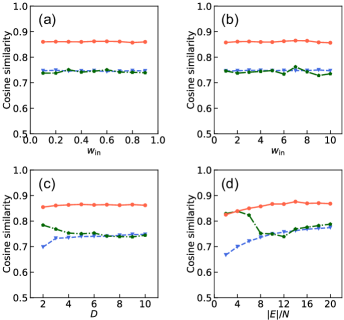
Figure S1: Comparison of the cosine similarity between the proposed model and the two baseline models when we vary a structural parameter for synthetic hypergraphs.

Figure S1 compares the cosine similarity between the proposed model and the two baseline models when we vary one of the structural parameters (i.e., $w_{\text{in}}$, $D$, or $|E|/N$) for synthetic hypergraphs.

S5 Cosine similarity for the HyCoSBM and HyperNEO when we vary the value of $\gamma$ in synthetic hypergraphs

We compute the average of the cosine similarity for the HyCoSBM [2] and HyperNEO over the 100 synthetic hypergraphs generated for a given combination $(p_{\bm{U}},w_{\text{in}},D,|E|/N)$. We set the hyperparameter $K=2$. We vary the value of the hyperparameter $\gamma$ from 0.1 to 0.9 in increments of 0.1 in both models.

Tables S1–S5 show the cosine similarity for the HyCoSBM and the HyperNEO with a given value of $\gamma$ when we vary one of the parameters for synthetic hypergraphs. We make the following observations. First, the proposed model with $\gamma=0.4$ or $\gamma=0.5$ achieves a higher value of the average cosine similarity over the different values of $p_{\bm{U}}$ (See Table S1). Second, the proposed model achieves the highest value of the average cosine similarity over the different values of any parameter for synthetic hypergraphs (see Tables S1–S5). Third, when we fix the value of a parameter for synthetic hypergraphs, the proposed model often achieves the highest value of the cosine similarity (see Tables S1–S5). Fourth, when we fix the value of $\gamma$ as 0.3, 0.4, or 0.5, the proposed model yields a higher value of the average cosine similarity over the different values of any parameter for synthetic hypergraphs than the HyCoSBM (see Tables S1–S5). Fifth, when we fix the value of $\gamma$ as 0.1, 0.2, 0.6, 0.7, 0.8, or 0.9, the proposed model yields a comparable or slightly lower value of the average cosine similarity over the different values of any parameter for synthetic hypergraphs than the HyCoSBM (see Tables S1–S5).

S6 Empirical hypergraphs

Table S6 shows the properties of the empirical hypergraphs. For any empirical hypergraph, the set $E$ contains a unique hyperedge, $e$, composed of the same set of nodes, and the number of times $e$ appears in the data set is stored in $A_{e}$.

S7 Hyperparameter tuning in empirical hypergraphs

Table S7 shows the tuned hyperparameter set for each model in each empirical hypergraph.

S8 Visualization of inferred membership and affinity matrices

Suppose that a given model produces inferred membership and affinity matrices, denoted by $(u_{ik})_{1\leq i\leq N,\ 1\leq k\leq K}$ and $(w_{kq})_{1\leq k\leq K,\ 1\leq q\leq K}$, respectively.

We perform the visualization of the inferred membership matrix as follows. First, we construct the normalized membership matrix $(u_{ik}^{\prime})_{1\leq i\leq N,\ 1\leq k\leq K}$, where we define $u_{ik}^{\prime}=u_{ik}/\sum_{k^{\prime}=1}^{K}u_{ik^{\prime}}$. This normalization is performed only for visualization purposes. Second, we arbitrarily fix the order of the indices of the $Z$ categories of the node attribute. Suppose that the order is given by $z_{1},\ldots,z_{Z}$, where $z_{l}\in\{1,\ldots,Z\}$ for any $l=1,\ldots,Z$. Third, we arrange the indices of the $N$ nodes according to their attributes as follows. We first arrange arbitrarily the indices of the nodes that have the attribute $z_{1}$. Then, for $l=2,\ldots,Z$ in order, we arrange arbitrarily the indices of the nodes that have the attribute $z_{l}$, and then, we place these indices behind the indices of the nodes that have the attribute $z_{l-1}$. In this way, we obtain the order of the indices of the $N$ nodes, denoted by $i_{1},\ldots,i_{N}$, where $i_{m}\in\{1,\ldots,N\}$ for any $m=1,\ldots,N$. Fourth, we arbitrarily fix the order of the indices of the $K$ communities. Suppose that the order is given by $k_{1},\ldots,k_{K}$, where $k_{n}\in\{1,\ldots,K\}$ for any $n=1,\ldots,K$. Finally, we visualize a heat map of the matrix $(u_{i_{m}k_{n}}^{\prime})_{1\leq m\leq N,\ 1\leq n\leq K}$.

We perform the visualization of the inferred affinity matrix as follows. We denote by $w_{\text{max}}$ is the largest element of the matrix. First, we calculate the normalized affinity matrix $(w_{kq}^{\prime})_{1\leq k\leq K,\ 1\leq q\leq K}$, where we define $w_{kq}^{\prime}=w_{kq}/w_{\text{max}}$. Then, we fix the same order of the indices of the $K$ communities, i.e., $k_{1},\ldots,k_{K}$, as that for the inferred membership matrix. We visualize a heat map of the matrix $(w_{k_{n}k_{n^{\prime}}}^{\prime})_{1\leq n\leq K,\ 1\leq n^{\prime}\leq K}$.

Figure S2 shows inferred affinity matrices of the three models in each empirical hypergraph.

S9 Other node layouts for empirical hypergraphs

To validate the node layouts obtained using the three stochastic block models, we show node layouts obtained using four baseline methods for each empirical hypergraph.

In the first baseline method, we apply the UMAP to the adjacency matrix, $\bm{A}=(a_{ij})_{1\leq i\leq N,\ 1\leq j\leq N}$, commonly defined for hypergraphs [3]. Formally, we define $a_{ij}$ as the number of hyperedges to which nodes $v_{i}$ and $v_{j}$ belong, i.e.,

$$a_{ij}=\sum_{e\in E,\ v_{i}\in e,\ v_{j}\in e}A_{e},$$ (S27)

for any $i=1,\ldots,N$ and any $j=1,\ldots,N$ such that $i\neq j$. We define $a_{ii}=0$ for any $i=1,\ldots,N$. We show in Fig. S3 UMAP projections of the adjacency matrix $\bm{A}$ in each empirical hypergraph. While the node layouts in each hypergraph are acceptable, the individuals are relatively sparsely distributed over the space in the workplace hypergraph (see Figs. S3(a) and S3(b))).

In the second baseline method, we use the adjacency matrix, $\bm{A}^{\prime}=(a^{\prime}_{ij})_{1\leq i\leq N,\ 1\leq j\leq N}$, where $(i,j)$-th entry is weighted by a factor that depends on the size of every hyperedge to which nodes $v_{i}$ and $v_{j}$ belong. We use $\kappa_{|e|}$, defined as Eq. (3), for the weight of given hyperedge $e$ [15]. We define

$$a^{\prime}_{ij}=\sum_{e\in E,\ v_{i}\in e,\ v_{j}\in e}\frac{A_{e}}{\kappa_{|e|}}$$ (S28)

for any $i=1,\ldots,N$ and any $j=1,\ldots,N$ such that $i\neq j$. We define $a^{\prime}_{ii}=0$ for any $i=1,\ldots,N$. We show in Fig. S4 UMAP projections of the adjacency matrix $\bm{A}^{\prime}$ in each empirical hypergraph. The individuals are positioned more closely to each other in the high-school and primary-school hypergraphs (see Figs. S4(e)–S4(h)), compared to the first baseline method; this result indicates the effectiveness of using the weight $\kappa_{|e|}$. On the other hand, the individuals are still relatively sparsely distributed over the space in the workplace hypergraph (see Figs. S4(a) and S4(b))).

In the third baseline method, we apply the UMAP to the attribute matrix $\bm{X}$. We use the Euclidean distance in the UMAP. Note that the set of coordinates obtained using the Euclidean distance in the UMAP is equivalent to that obtained using the cosine distance in the UMAP. This is because it holds true that $\sum_{z=1}^{Z}x_{iz}=1$ for any $i=1,\ldots,N$. This method is similar to that used in Ref. [16] in that we apply a dimensionality reduction method to the representation of node attributes. We show in Fig. S5 a UMAP projection of the matrix $\bm{X}$ in each empirical hypergraph. This method is expected to perform well when node attributes align with the communities. However, node attributes do not always align with the communities in empirical networks [13]. In fact, the students are sparsely distributed over the space in the high-school hypergraph (see Fig. S5(d)).

In the fourth baseline method, we use the Fruchterman-Reingold force-directed algorithm [8] to map nodes into a two-dimensional vector space. This method has been deployed in the library ‘Hypergraphx’ for the visualization of a hypergraph [11]. To deploy this algorithm to an empirical hypergraph, we first construct the one-mode projected network in which two nodes $v_{i}$ and $v_{j}\ (i\neq j)$ are connected by an undirected edge $(v_{i},v_{j})$ with the weight $a_{ij}$ if they share one or more hyperedges. Then, we obtain a set of coordinates of the nodes by applying the Fruchterman-Reingold force-directed algorithm to the projected network. To this end, we use ‘spring_layout’ function setting default parameters in the ‘NetworkX’ library [1]. We show in Fig. S6 a force-directed layout of the nodes in each empirical hypergraph. While the node layout in each hypergraph is acceptable, it seems to be easier to find individuals who have similar community memberships in the space using stochastic block models than using the force-directed algorithm.

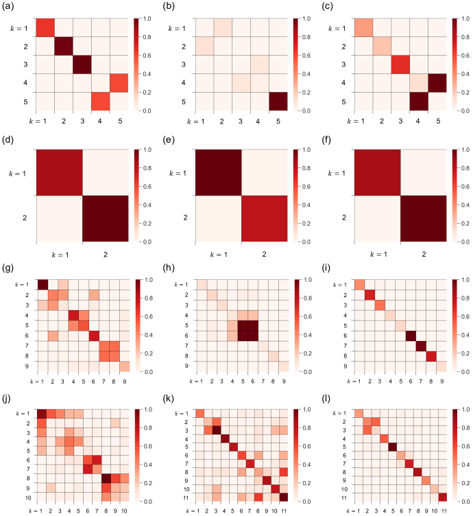
Figure S2: Inferred affinity matrices in each empirical hypergraph. Panels (a)–(c) show the results for the workplace hypergraph, panels (d)–(f) show the results for the hospital hypergraph, panels (g)–(i) show the results for the high-school hypergraph, and panels (j)–(l) show the results for the primary-school hypergraph. The results for the Hy-MMSBM are shown in (a), (d), (g), and (j), those for the HyCoSBM are shown in (b), (e), (h), and (k), and those for the proposed model are shown in (c), (f), (i), and (l).

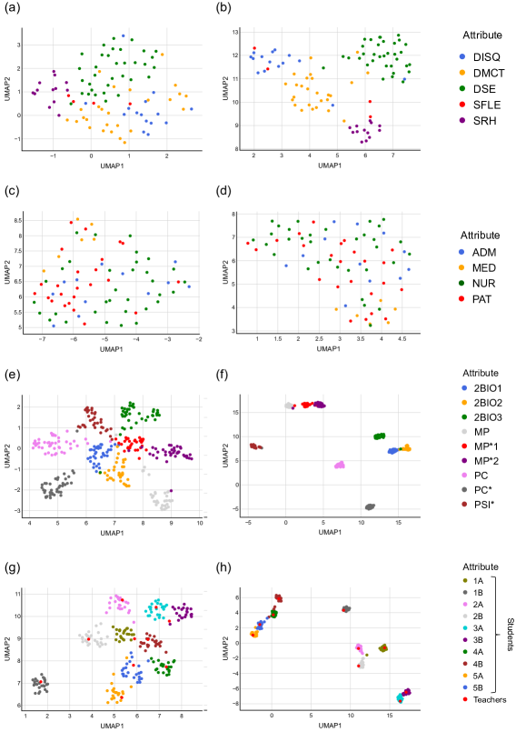
Figure S3: UMAP projections of the representation $\bm{A}$ for each empirical hypergraph. Panels (a) and (b): workplace hypergraph. Panels (c) and (d): hospital hypergraph. Panels (e) and (f): high-school hypergraph. Panels (g) and (h): primary-school hypergraph. We use the Euclidean distance in (a), (c), (e), and (g) and the cosine distance in (b), (d), (f), and (h) in the UMAP.

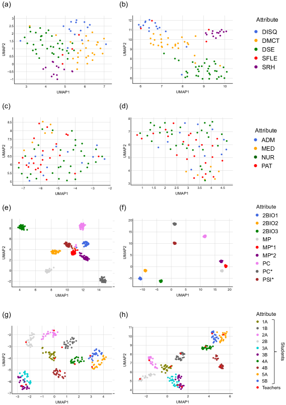
Figure S4: UMAP projections of the representation $\bm{A}^{\prime}$ in each empirical hypergraph. Panels (a) and (b): workplace hypergraph. Panels (c) and (d): hospital hypergraph. Panels (e) and (f): high-school hypergraph. Panels (g) and (h): primary-school hypergraph. We use the Euclidean distance in (a), (c), (e), and (g) and the cosine distance in (b), (d), (f), and (h) in the UMAP.

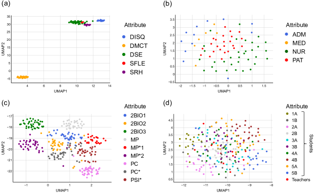
Figure S5: UMAP projection of the representation $\bm{X}$ in each empirical hypergraph. Panel (a): workplace hypergraph. Panel (b): hospital hypergraph. Panel (c): high-school hypergraph. Panel (d): primary-school hypergraph.

Figure S6: Force-directed layout of the one-mode projected network for each empirical hypergraph. Panel (a): workplace hypergraph. Panel (b): hospital hypergraph. Panel (c): high-school hypergraph. Panel (d): primary-school hypergraph.

Table S1: Cosine similarity for the HyCoSBM and HyperNEO with a given value of the hyperparameter $\gamma$ when we vary $p_{\bm{U}}$. In Tables S1–S5, the rightmost column shows the average of the cosine similarity of a model with a given value of $\gamma$ across the different values of a given parameter for synthetic hypergraphs, and the highest value in each column is indicated in bold.

Model	$p_{\bm{U}}$						Mean
	0.5	0.6	0.7	0.8	0.9	1.0
HyCoSBM
$\gamma=0.1$	0.869	0.853	0.815	0.754	0.693	0.641	0.771
$0.2$	0.873	0.855	0.821	0.769	0.714	0.681	0.785
$0.3$	0.854	0.847	0.810	0.773	0.715	0.699	0.783
$0.4$	0.826	0.812	0.795	0.759	0.699	0.675	0.761
$0.5$	0.796	0.786	0.769	0.754	0.743	0.743	0.765
$0.6$	0.770	0.783	0.805	0.845	0.892	0.971	0.844
$0.7$	0.728	0.738	0.778	0.837	0.910	0.998	0.831
$0.8$	0.719	0.731	0.772	0.827	0.906	0.999	0.826
$0.9$	0.709	0.723	0.766	0.825	0.904	0.999	0.821
HyperNEO
$\gamma=0.1$	0.865	0.851	0.809	0.753	0.691	0.633	0.767
$0.2$	0.866	0.853	0.818	0.765	0.712	0.671	0.781
$0.3$	0.864	0.852	0.828	0.796	0.757	0.772	0.811
$0.4$	0.846	0.845	0.846	0.855	0.869	0.918	0.863
$0.5$	0.794	0.806	0.828	0.864	0.910	0.970	0.862
$0.6$	0.745	0.758	0.793	0.845	0.918	0.992	0.842
$0.7$	0.719	0.732	0.772	0.828	0.910	0.999	0.827
$0.8$	0.709	0.723	0.761	0.823	0.909	0.999	0.821
$0.9$	0.707	0.723	0.764	0.828	0.905	0.999	0.821

Table S2: Cosine similarity for the HyCoSBM and HyperNEO when we vary $\gamma$ and $w_{\text{in}}$, where $w_{\text{in}}<1.0$.

Model	$w_{\text{in}}$									Mean
	0.1	0.2	0.3	0.4	0.5	0.6	0.7	0.8	0.9
HyCoSBM
$\gamma=0.1$	0.758	0.755	0.756	0.753	0.754	0.753	0.756	0.754	0.754	0.755
$0.2$	0.767	0.769	0.765	0.768	0.765	0.764	0.765	0.765	0.770	0.766
$0.3$	0.766	0.765	0.765	0.765	0.767	0.760	0.767	0.770	0.766	0.766
$0.4$	0.746	0.743	0.758	0.749	0.754	0.733	0.753	0.742	0.754	0.748
$0.5$	0.738	0.738	0.751	0.742	0.745	0.751	0.742	0.741	0.739	0.743
$0.6$	0.840	0.838	0.840	0.850	0.846	0.847	0.850	0.844	0.836	0.843
$0.7$	0.832	0.835	0.837	0.832	0.830	0.835	0.835	0.832	0.834	0.834
$0.8$	0.834	0.830	0.832	0.830	0.829	0.830	0.832	0.827	0.829	0.830
$0.9$	0.823	0.823	0.827	0.824	0.828	0.825	0.835	0.827	0.828	0.827
HyperNEO
$\gamma=0.1$	0.751	0.751	0.751	0.753	0.752	0.754	0.751	0.750	0.751	0.752
$0.2$	0.763	0.761	0.766	0.761	0.763	0.763	0.760	0.762	0.761	0.762
$0.3$	0.794	0.794	0.793	0.794	0.793	0.795	0.798	0.789	0.791	0.793
$0.4$	0.853	0.855	0.858	0.851	0.855	0.856	0.853	0.841	0.847	0.852
$0.5$	0.860	0.861	0.861	0.860	0.862	0.862	0.861	0.857	0.860	0.861
$0.6$	0.841	0.846	0.845	0.846	0.849	0.842	0.845	0.845	0.845	0.845
$0.7$	0.833	0.833	0.835	0.833	0.827	0.826	0.829	0.834	0.832	0.831
$0.8$	0.825	0.832	0.825	0.823	0.825	0.831	0.828	0.823	0.828	0.827
$0.9$	0.826	0.828	0.823	0.823	0.820	0.824	0.826	0.822	0.823	0.824

Table S3: Cosine similarity for the HyCoSBM and HyperNEO when we vary $\gamma$ and $w_{\text{in}}$, where $w_{\text{in}}\geq 1.0$.

Model	$w_{\text{in}}$										Mean
	1.0	2.0	3.0	4.0	5.0	6.0	7.0	8.0	9.0	10.0
HyCoSBM
$\gamma=0.1$	0.757	0.755	0.753	0.755	0.755	0.756	0.754	0.755	0.756	0.754	0.755
$0.2$	0.767	0.771	0.766	0.769	0.767	0.765	0.772	0.768	0.769	0.769	0.768
$0.3$	0.765	0.765	0.767	0.766	0.765	0.767	0.763	0.767	0.768	0.770	0.766
$0.4$	0.747	0.759	0.760	0.772	0.747	0.746	0.758	0.769	0.748	0.747	0.755
$0.5$	0.746	0.738	0.741	0.744	0.748	0.734	0.762	0.743	0.728	0.735	0.742
$0.6$	0.841	0.841	0.850	0.845	0.847	0.845	0.845	0.855	0.847	0.845	0.846
$0.7$	0.835	0.834	0.841	0.836	0.834	0.837	0.836	0.836	0.836	0.838	0.836
$0.8$	0.838	0.832	0.832	0.830	0.830	0.834	0.826	0.827	0.827	0.828	0.830
$0.9$	0.827	0.830	0.825	0.829	0.825	0.826	0.826	0.826	0.825	0.831	0.827
HyperNEO
$\gamma=0.1$	0.752	0.751	0.753	0.751	0.751	0.752	0.753	0.752	0.751	0.752	0.752
$0.2$	0.764	0.766	0.764	0.765	0.766	0.764	0.761	0.766	0.761	0.763	0.764
$0.3$	0.796	0.794	0.797	0.798	0.798	0.793	0.795	0.791	0.802	0.795	0.796
$0.4$	0.850	0.848	0.850	0.850	0.851	0.843	0.854	0.855	0.859	0.847	0.851
$0.5$	0.858	0.861	0.862	0.860	0.859	0.863	0.865	0.864	0.858	0.857	0.861
$0.6$	0.846	0.842	0.845	0.840	0.847	0.846	0.846	0.846	0.839	0.848	0.844
$0.7$	0.833	0.832	0.832	0.835	0.829	0.832	0.831	0.835	0.828	0.833	0.832
$0.8$	0.822	0.825	0.829	0.824	0.828	0.826	0.828	0.827	0.822	0.829	0.826
$0.9$	0.824	0.830	0.826	0.829	0.825	0.820	0.828	0.826	0.818	0.820	0.825

Table S4: Cosine similarity for the HyCoSBM and HyperNEO when we vary $\gamma$ and $D$.

Model	$D$									Mean
	2	3	4	5	6	7	8	9	10
HyCoSBM
$\gamma=0.1$	0.748	0.741	0.744	0.743	0.746	0.750	0.752	0.755	0.758	0.749
$0.2$	0.755	0.753	0.755	0.758	0.758	0.765	0.763	0.770	0.772	0.761
$0.3$	0.753	0.754	0.759	0.760	0.759	0.756	0.770	0.757	0.768	0.760
$0.4$	0.741	0.738	0.743	0.743	0.753	0.753	0.773	0.736	0.760	0.749
$0.5$	0.784	0.769	0.753	0.750	0.753	0.741	0.739	0.738	0.744	0.752
$0.6$	0.855	0.844	0.851	0.854	0.841	0.850	0.847	0.843	0.846	0.848
$0.7$	0.848	0.843	0.844	0.833	0.835	0.836	0.835	0.830	0.830	0.837
$0.8$	0.843	0.838	0.841	0.834	0.834	0.827	0.835	0.831	0.832	0.835
$0.9$	0.842	0.833	0.827	0.828	0.821	0.828	0.827	0.825	0.829	0.829
HyperNEO
$\gamma=0.1$	0.749	0.740	0.741	0.741	0.745	0.746	0.748	0.750	0.751	0.745
$0.2$	0.755	0.750	0.749	0.755	0.754	0.757	0.759	0.762	0.766	0.756
$0.3$	0.777	0.767	0.769	0.773	0.776	0.784	0.789	0.791	0.794	0.780
$0.4$	0.798	0.799	0.807	0.816	0.826	0.839	0.840	0.842	0.847	0.824
$0.5$	0.855	0.861	0.863	0.865	0.863	0.864	0.862	0.865	0.862	0.862
$0.6$	0.847	0.854	0.841	0.848	0.844	0.846	0.848	0.848	0.849	0.847
$0.7$	0.832	0.835	0.834	0.829	0.830	0.834	0.833	0.833	0.830	0.832
$0.8$	0.827	0.823	0.827	0.825	0.830	0.829	0.825	0.825	0.828	0.827
$0.9$	0.825	0.824	0.830	0.825	0.827	0.825	0.824	0.826	0.824	0.825

Table S5: Cosine similarity for the HyCoSBM and HyperNEO when we vary $\gamma$ and $|E|/N$.

Model	$|E|/N$										Mean
	2	4	6	8	10	12	14	16	18	20
HyCoSBM
$\gamma=0.1$	0.713	0.720	0.733	0.747	0.755	0.762	0.767	0.774	0.775	0.778	0.752
$0.2$	0.681	0.734	0.753	0.760	0.767	0.776	0.779	0.783	0.784	0.788	0.760
$0.3$	0.768	0.704	0.732	0.752	0.762	0.776	0.780	0.790	0.786	0.787	0.764
$0.4$	0.832	0.766	0.718	0.737	0.746	0.766	0.780	0.788	0.782	0.790	0.771
$0.5$	0.829	0.838	0.823	0.752	0.750	0.739	0.769	0.776	0.782	0.788	0.785
$0.6$	0.829	0.834	0.831	0.842	0.834	0.823	0.802	0.792	0.787	0.784	0.816
$0.7$	0.827	0.827	0.833	0.829	0.832	0.837	0.849	0.850	0.857	0.848	0.839
$0.8$	0.824	0.824	0.831	0.828	0.829	0.830	0.837	0.833	0.834	0.840	0.831
$0.9$	0.821	0.825	0.825	0.826	0.829	0.826	0.829	0.829	0.827	0.826	0.826
HyperNEO
$\gamma=0.1$	0.705	0.715	0.730	0.741	0.753	0.758	0.766	0.769	0.774	0.777	0.749
$0.2$	0.793	0.758	0.756	0.760	0.764	0.769	0.773	0.774	0.778	0.780	0.771
$0.3$	0.832	0.826	0.814	0.802	0.799	0.791	0.788	0.792	0.791	0.790	0.802
$0.4$	0.836	0.842	0.855	0.857	0.850	0.841	0.833	0.835	0.823	0.820	0.839
$0.5$	0.825	0.839	0.850	0.857	0.867	0.867	0.876	0.869	0.870	0.868	0.859
$0.6$	0.825	0.827	0.832	0.832	0.843	0.847	0.861	0.868	0.870	0.872	0.848
$0.7$	0.828	0.824	0.826	0.824	0.832	0.838	0.837	0.845	0.848	0.857	0.836
$0.8$	0.827	0.826	0.823	0.828	0.822	0.826	0.825	0.835	0.825	0.835	0.827
$0.9$	0.829	0.820	0.824	0.822	0.825	0.821	0.821	0.827	0.828	0.822	0.824

Table S6: Properties of the empirical hypergraphs. $N$: number of nodes, $|E|$: number of hyperedges, $\bar{k}$: average degree of the node, $\bar{s}$: average size of the hyperedge, $D$: maximum size of the hyperedge, and $Z$: number of categories of the node attribute.

Data	$N$	$|E|$	$\bar{k}$	$\bar{s}$	$D$	$Z$	References
workplace	92	788	17.7	2.1	4	5	[10, 15]
hospital	75	1,825	59.1	2.4	5	4	[18, 15]
high-school	327	7,818	55.6	2.3	5	9	[12, 5, 4]
primary-school	242	12,704	127.0	2.4	5	11	[17, 9, 5, 4]

Table S7: Tuned hyperparameter set for each model in the empirical hypergraphs.

Data	Hy-MMSBM	HyCoSBM	HyperNEO
	$K$	($K,\gamma$)	($K,\gamma$)
workplace	5	(5, 0.9)	(5, 0.9)
hospital	2	(2, 0.2)	(2, 0.4)
high-school	9	(9, 0.9)	(9, 0.8)
primary-school	10	(11, 0.9)	(11, 0.8)

References

- [1] UMAP: Uniform manifold approximation and projection for dimension reduction. https://umap-learn.readthedocs.io/en/latest/. Accessed November 2023.
- [2] Christopher Aicher, Abigail Z. Jacobs, and Aaron Clauset. Learning latent block structure in weighted networks. Journal of Complex Networks, 3:221–248, 2014.
- [3] Edo M Airoldi, David Blei, Stephen Fienberg, and Eric Xing. Mixed membership stochastic blockmodels. Journal of Machine Learning Research, 9:1981–2014, 2008.
- [4] Unai Alvarez-Rodriguez, Federico Battiston, Guilherme Ferraz de Arruda, Yamir Moreno, Matjaž Perc, and Vito Latora. Evolutionary dynamics of higher-order interactions in social networks. Nature Human Behaviour, 5:586–595, 2021.
- [5] Ilya Amburg, Nate Veldt, and Austin Benson. Clustering in graphs and hypergraphs with categorical edge labels. In Proceedings of The Web Conference 2020, page 706â717, 2020.
- [6] Anna Badalyan, Nicolò Ruggeri, and Caterina De Bacco. Hypergraphs with node attributes: structure and inference. arXiv preprint arXiv:2311.03857, 2023.
- [7] Brian Ball, Brian Karrer, and M. E. J. Newman. Efficient and principled method for detecting communities in networks. Physical Review E, 84:036103, 2011.
- [8] A. Barrat, M. Barthélemy, and A. Vespignani. Dynamical Processes on Complex Networks. Cambridge University Press, Cambridge, UK, 2008.
- [9] Aleix Bassolas, Anton Holmgren, Antoine Marot, Martin Rosvall, and Vincenzo Nicosia. Mapping nonlocal relationships between metadata and network structure with metadata-dependent encoding of random walks. Science Advances, 8:eabn7558, 2022.
- [10] F. Battiston, G. Cencetti, I. Iacopini, V. Latora, M. Lucas, A. Patania, J.-G. Young, and G. Petri. Networks beyond pairwise interactions: Structure and dynamics. Physics Reports, 874:1–92, 2020.
- [11] Federico Battiston, Enrico Amico, Alain Barrat, Ginestra Bianconi, Guilherme Ferraz de Arruda, Benedetta Franceschiello, Iacopo Iacopini, Sonia Kéfi, Vito Latora, Yamir Moreno, Micah M. Murray, Tiago P. Peixoto, Francesco Vaccarino, and Giovanni Petri. The physics of higher-order interactions in complex systems. Nature Physics, 17:1093–1098, 2021.
- [12] Etienne Becht, Leland McInnes, John Healy, Charles-Antoine Dutertre, Immanuel W H Kwok, Lai Guan Ng, Florent Ginhoux, and Evan W Newell. Dimensionality reduction for visualizing single-cell data using umap. Nature Biotechnology, 37:38–44, 2019.
- [13] Mikhail Belkin and Partha Niyogi. Laplacian eigenmaps and spectral techniques for embedding and clustering. In T. Dietterich, S. Becker, and Z. Ghahramani, editors, Advances in Neural Information Processing Systems, volume 14, 2001.
- [14] Alexandre Benatti, Henrique Ferraz de Arruda, Filipi Nascimento Silva, César Henrique Comin, and Luciano da Fontoura Costa. On the stability of citation networks. Physica A: Statistical Mechanics and its Applications, 610:128399, 2023.
- [15] Austin R. Benson. https://www.cs.cornell.edu/~arb/data/. Accessed September 2023.
- [16] Kenneth S. Berenhaut, Katherine E. Moore, and Ryan L. Melvin. A social perspective on perceived distances reveals deep community structure. Proceedings of the National Academy of Sciences of the United States of America, 119:e2003634119, 2022.
- [17] Ginestra Bianconi. Higher-Order Networks. Elements in the Structure and Dynamics of Complex Networks. Cambridge University Press, 2021.
- [18] Christian Bick, Elizabeth Gross, Heather A. Harrington, and Michael T. Schaub. What are higher-order networks? SIAM Review, 65:686–731, 2023.
- [19] S. Boccaletti, P. De Lellis, C.I. del Genio, K. Alfaro-Bittner, R. Criado, S. Jalan, and M. Romance. The structure and dynamics of networks with higher order interactions. Physics Reports, 1018:1–64, 2023.
- [20] S. Boccaletti, V. Latora, Y. Moreno, M. Chavez, and D.-U. Hwang. Complex networks: Structure and dynamics. Physics Reports, 424:175–308, 2006.
- [21] Timoteo Carletti, Duccio Fanelli, and Renaud Lambiotte. Random walks and community detection in hypergraphs. Journal of Physics: Complexity, 2:015011, 2021.
- [22] I Chien, Chung-Yi Lin, and I-Hsiang Wang. Community detection in hypergraphs: Optimal statistical limit and efficient algorithms. In Proceedings of the Twenty-First International Conference on Artificial Intelligence and Statistics, volume 84, pages 871–879, 2018.
- [23] Philip S. Chodrow, Nate Veldt, and Austin R. Benson. Generative hypergraph clustering: From blockmodels to modularity. Science Advances, 7:eabh1303, 2021.
- [24] Petr Chunaev. Community detection in node-attributed social networks: A survey. Computer Science Review, 37:100286, 2020.
- [25] Martina Contisciani, Federico Battiston, and Caterina De Bacco. Inference of hyperedges and overlapping communities in hypergraphs. Nature Communications, 13:7229, 2022.
- [26] Martina Contisciani, Eleanor A. Power, and Caterina De Bacco. Community detection with node attributes in multilayer networks. Scientific Reports, 10:15736, 2020.
- [27] Caterina De Bacco, Eleanor A. Power, Daniel B. Larremore, and Cristopher Moore. Community detection, link prediction, and layer interdependence in multilayer networks. Physical Review E, 95:042317, 2017.
- [28] A. P. Dempster, N. M. Laird, and D. B. Rubin. Maximum likelihood from incomplete data via the em algorithm. Journal of the Royal Statistical Society: Series B (Methodological), 39:1–22, 1977.
- [29] Anton Eriksson, Daniel Edler, Alexis Rojas, Manlio de Domenico, and Martin Rosvall. How choosing random-walk model and network representation matters for flow-based community detection in hypergraphs. Communications Physics, 4:133, 2021.
- [30] Santo Fortunato. Community detection in graphs. Physics Reports, 486:75–174, 2010.
- [31] Santo Fortunato and Darko Hric. Community detection in networks: A user guide. Physics Reports, 659:1–44, 2016.
- [32] Santo Fortunato and Mark E. J. Newman. 20 years of network community detection. Nature Physics, 18:848–850, 2022.
- [33] Thomas M. J. Fruchterman and Edward M. Reingold. Graph drawing by force-directed placement. Software: Practice and Experience, 21:1129–1164, 1991.
- [34] Valerio Gemmetto, Alain Barrat, and Ciro Cattuto. Mitigation of infectious disease at school: targeted class closure vs school closure. BMC Infectious Diseases, 14:695, 2014.
- [35] Mathieu Génois, Christian L Vestergaard, Julie Fournet, André Panisson, Isabelle Bonmarin, and Alain Barrat. Data on face-to-face contacts in an office building suggest a low-cost vaccination strategy based on community linkers. Network Science, 3:326â347, 2015.
- [36] Amir Ghasemian, Homa Hosseinmardi, and Aaron Clauset. Evaluating overfit and underfit in models of network community structure. IEEE Transactions on Knowledge and Data Engineering, 32:1722–1735, 2020.
- [37] Prem K. Gopalan and David M. Blei. Efficient discovery of overlapping communities in massive networks. Proceedings of the National Academy of Sciences of the United States of America, 110:14534–14539, 2013.
- [38] Paul W. Holland, Kathryn Blackmond Laskey, and Samuel Leinhardt. Stochastic blockmodels: First steps. Social Networks, 5:109–137, 1983.
- [39] Darko Hric, Tiago P. Peixoto, and Santo Fortunato. Network structure, metadata, and the prediction of missing nodes and annotations. Physical Review X, 6:031038, 2016.
- [40] Brian Karrer and M. E. J. Newman. Stochastic blockmodels and community structure in networks. Physical Review E, 83:016107, 2011.
- [41] Zheng Tracy Ke, Feng Shi, and Dong Xia. Community detection for hypergraph networks via regularized tensor power iteration. arXiv preprint arXiv:1909.06503, 2019.
- [42] Chiheon Kim, Afonso S. Bandeira, and Michel X. Goemans. Community detection in hypergraphs, spiked tensor models, and sum-of-squares. In 2017 International Conference on Sampling Theory and Applications (SampTA), pages 124–128, 2017.
- [43] Daniel B. Larremore, Aaron Clauset, and Abigail Z. Jacobs. Efficiently inferring community structure in bipartite networks. Physical Review E, 90:012805, 2014.
- [44] V. Latora, V. Nicosia, and G. Russo. Complex Networks: Principles, Methods and Applications. Cambridge University Press, Cambridge, UK, 2017.
- [45] Clement Lee and Darren J. Wilkinson. A review of stochastic block models and extensions for graph clustering. Applied Network Science, 4(1):122, 2019.
- [46] Ye Li, Chaofeng Sha, Xin Huang, and Yanchun Zhang. Community detection in attributed graphs: An embedding approach. Proceedings of the AAAI Conference on Artificial Intelligence, 32, 2018.
- [47] Quintino Francesco Lotito, Martina Contisciani, Caterina De Bacco, Leonardo Di Gaetano, Luca Gallo, Alberto Montresor, Federico Musciotto, Nicolò Ruggeri, and Federico Battiston. Hypergraphx: a library for higher-order network analysis. Journal of Complex Networks, 11:cnad019, 2023.
- [48] Quintino Francesco Lotito, Federico Musciotto, Alberto Montresor, and Federico Battiston. Higher-order motif analysis in hypergraphs. Communications Physics, 5(1), 2022.
- [49] Quintino Francesco Lotito, Federico Musciotto, Alberto Montresor, and Federico Battiston. Hyperlink communities in higher-order networks. arXiv preprint arXiv:2303.01385, 2023.
- [50] Soumen Majhi, Matjaž Perc, and Dibakar Ghosh. Dynamics on higher-order networks: A review. Journal of The Royal Society Interface, 19:20220043, 2022.
- [51] Rossana Mastrandrea, Julie Fournet, and Alain Barrat. Contact patterns in a high school: A comparison between data collected using wearable sensors, contact diaries and friendship surveys. PLOS ONE, 10:e0136497, 2015.
- [52] Leland McInnes, John Healy, Nathaniel Saul, and Lukas GroÃberger. UMAP: Uniform manifold approximation and projection. Journal of Open Source Software, 3:861, 2018.
- [53] Dakota Murray, Jisung Yoon, Sadamori Kojaku, Rodrigo Costas, Woo-Sung Jung, StaÅ¡a MilojeviÄ, and Yong-Yeol Ahn. Unsupervised embedding of trajectories captures the latent structure of scientific migration. Proceedings of the National Academy of Sciences of the United States of America, 120:e2305414120, 2023.
- [54] Kazuki Nakajima, Ruodan Liu, Kazuyuki Shudo, and Naoki Masuda. Quantifying gender imbalance in east asian academia: Research career and citation practice. Journal of Informetrics, 17:101460, 2023.
- [55] Kazuki Nakajima, Kazuyuki Shudo, and Naoki Masuda. Higher-order rich-club phenomenon in collaborative research grant networks. Scientometrics, 128(4):2429–2446, 2023.
- [56] M. E. J. Newman. The structure of scientific collaboration networks. Proceedings of the National Academy of Sciences of the United States of America, 98:404–409, 2001.
- [57] M. E. J. Newman. Networks. Second Edition. Oxford University Press, Oxford, UK, 2018.
- [58] M. E. J. Newman and Aaron Clauset. Structure and inference in annotated networks. Nature Communications, 7(1):11863, 2016.
- [59] M. E. J. Newman and M. Girvan. Finding and evaluating community structure in networks. Physical Review E, 69:026113, 2004.
- [60] Gergely Palla, Imre Derényi, Illés Farkas, and Tamás Vicsek. Uncovering the overlapping community structure of complex networks in nature and society. Nature, 435:814–818, 2005.
- [61] Raj Kumar Pan, Kimmo Kaski, and Santo Fortunato. World citation and collaboration networks: uncovering the role of geography in science. Scientific Reports, 2:902, 2012.
- [62] A. Patania, G. Petri, and F. Vaccarino. The shape of collaborations. EPJ Data Science, 6, 2017. Art. no. 18.
- [63] Leto Peel, Daniel B. Larremore, and Aaron Clauset. The ground truth about metadata and community detection in networks. Science Advances, 3:e1602548, 2017.
- [64] Ludovic Rheault and Andreea Musulan. Efficient detection of online communities and social bot activity during electoral campaigns. Journal of Information Technology & Politics, 18:324–337, 2021.
- [65] Nicolò Ruggeri, Federico Battiston, and Caterina De Bacco. A framework to generate hypergraphs with community structure. arXiv preprint arXiv:2212.08593, 2023. DOI: 10.48550/arXiv.2212.08593.
- [66] Nicolò Ruggeri, Martina Contisciani, Federico Battiston, and Caterina De Bacco. Community detection in large hypergraphs. Science Advances, 9:eadg9159, 2023.
- [67] Marta Sales-Pardo, Aleix Mariné-Tena, and Roger Guimerà . Hyperedge prediction and the statistical mechanisms of higher-order and lower-order interactions in complex networks. Proceedings of the National Academy of Sciences of the United States of America, 120:e2303887120, 2023.
- [68] Natalie Stanley, Thomas Bonacci, Roland Kwitt, Marc Niethammer, and Peter J. Mucha. Stochastic block models with multiple continuous attributes. Applied Network Science, 4(1):54, 2019.
- [69] Juliette Stehlé, Nicolas Voirin, Alain Barrat, Ciro Cattuto, Lorenzo Isella, Jean-François Pinton, Marco Quaggiotto, Wouter Van den Broeck, Corinne Régis, Bruno Lina, and Philippe Vanhems. High-resolution measurements of face-to-face contact patterns in a primary school. PLOS ONE, 6:e23176, 2011.
- [70] Joshua B. Tenenbaum, Vin de Silva, and John C. Langford. A global geometric framework for nonlinear dimensionality reduction. Science, 290:2319–2323, 2000.
- [71] Leo Torres, Ann S. Blevins, Danielle Bassett, and Tina Eliassi-Rad. The why, how, and when of representations for complex systems. SIAM Review, 63:435–485, 2021.
- [72] Taro Ueno and Naoki Masuda. Controlling nosocomial infection based on structure of hospital social networks. Journal of Theoretical Biology, 254:655–666, 2008.
- [73] Laurens van der Maaten and Geoffrey Hinton. Visualizing data using t-sne. Journal of Machine Learning Research, 9:2579–2605, 2008.
- [74] Philippe Vanhems, Alain Barrat, Ciro Cattuto, Jean-François Pinton, Nagham Khanafer, Corinne Régis, Byeul-a Kim, Brigitte Comte, and Nicolas Voirin. Estimating potential infection transmission routes in hospital wards using wearable proximity sensors. PLOS ONE, 8:e73970, 2013.
- [75] Xiao Wang, Di Jin, Xiaochun Cao, Liang Yang, and Weixiong Zhang. Semantic community identification in large attribute networks. Proceedings of the AAAI Conference on Artificial Intelligence, 30, 2016.
- [76] C. F. Jeff Wu. On the convergence properties of the EM algorithm. The Annals of Statistics, 11:95–103, 1983.
- [77] Jaewon Yang, Julian McAuley, and Jure Leskovec. Community detection in networks with node attributes. In 2013 IEEE 13th International Conference on Data Mining, pages 1151–1156, 2013.
- [78] Jaewon Yang, Julian McAuley, and Jure Leskovec. Detecting cohesive and 2-mode communities indirected and undirected networks. In Proceedings of the 7th ACM International Conference on Web Search and Data Mining, page 323â332, 2014.
- [79] Yaoming Zhen and Junhui Wang. Community detection in general hypergraph via graph embedding. Journal of the American Statistical Association, 118:1620–1629, 2023.
- [80] Dengyong Zhou, Jiayuan Huang, and Bernhard Schölkopf. Learning with hypergraphs: Clustering, classification, and embedding. In Advances in Neural Information Processing Systems, volume 19, 2006.
- [81] Youjia Zhou, Archit Rathore, Emilie Purvine, and Bei Wang. Topological simplifications of hypergraphs. IEEE Transactions on Visualization and Computer Graphics, 29:3209–3225, 2023.