Adversarially Trained Actor Critic for offline CMDPs

Abstract

We propose a Safe Adversarial Trained Actor Critic (SATAC) algorithm for offline reinforcement learning (RL) with general function approximation in the presence of limited data coverage. SATAC operates as a two-player Stackelberg game featuring a refined objective function. The actor (leader player) optimizes the policy against two adversarially trained value critics (follower players), who focus on scenarios where the actor’s performance is inferior to the behavior policy. Our framework provides both theoretical guarantees and a robust deep-RL implementation. Theoretically, we demonstrate that when the actor employs a no-regret optimization oracle, SATAC achieves two guarantees: $(i)$ For the first time in the offline RL setting, we establish that SATAC can produce a policy that outperforms the behavior policy while maintaining the same level of safety, which is critical to designing an algorithm for offline RL. $(ii)$ We demonstrate that the algorithm guarantees policy improvement across a broad range of hyperparameters, indicating its practical robustness. Additionally, we offer a practical version of SATAC and compare it with existing state-of-the-art offline safe-RL algorithms in continuous control environments. SATAC outperforms all baselines across a range of tasks, thus validating the theoretical performance.

1 INTRODUCTION

Online safe reinforcement learning (RL) has found successful applications in various domains, such as autonomous driving (Isele et al.,, 2018), recommender systems (Chow et al.,, 2017), and robotics (Achiam et al.,, 2017). It enables the learning of safe policies that perform effectively while satisfying multiple safety constraints, including collision avoidance, budget adherence, and reliability. However, collecting diverse interaction data can be prohibitively expensive or infeasible in many real-world applications, and this challenge becomes even more critical in the context of safe RL. Especially in scenarios where safety is of utmost importance, the cost associated with any form of risky behavior cannot be tolerated. Given the inherently risk-sensitive nature of these safety-related tasks, data collection becomes feasible only when employing behavior policies that conform to specific baseline performance or safety requirements.

To overcome the limitations imposed by interactive data collection, offline RL algorithms are designed to learn a policy from an available dataset collected from historical experiences by some behavior policies, which may differ from the policy we aim to learn. As discussed in Cheng et al., (2022), an offline RL algorithm should produce a policy that outperforms the behavior policy used to collect the data and should have the capability to learn other policies when the state-action distribution is sufficiently covered. These advantages become even more crucial in the context of safe offline RL. For instance, in autonomous driving, the ideal scenario involves having a defensive human driver operate the vehicle to accumulate a diverse dataset under various road and weather conditions, serving as the behavior policy. This behavior policy can be considered good since it adheres to all traffic rules. Subsequently, we can train an improved policy while ensuring at least the same level of safety using this historical data. This approach can significantly mitigate the potential collisions and safety issues that might arise if autonomous vehicles were to explore the environment directly.

However, unlike online safe-RL (Brantley et al.,, 2020; Efroni et al., 2020a, ; Wei et al., 2022b, ; Wei et al., 2022a, ; Liu et al.,, 2021; Bura et al.,, 2021; Singh et al.,, 2020; Ding et al.,, 2021; Chen et al., 2022b, ; Ding and Lavaei,, 2022; Wei et al.,, 2023; WeiLiuYin_24), as far as we know, existing theoretical studies on offline safe-RL are quite limited. The following questions arise:

$(1)$ Can we guarantee an improvement in performance over the behavior policy while maintaining safety?
$(2)$ Under what conditions can we learn the optimal and safe policy?

We answer these questions affirmatively by proposing a new model-free offline safe-RL algorithm, Safe Adversarially Trained Actor Critic (SATAC). SATAC is designed based on a refined Stackelberg game theoretical (Von Stackelberg,, 2010) formulation of offline safe-RL. The actor acts as the leader player to perform well and safe over two follower critics (one for reward and one for cost). The two critics are adversarially trained to find scenarios that the actor acts worse than the behavior policy. Our main contributions are summarized below:

• We prove that under standard function approximation assumptions, when the actor employs a no-regret policy optimization oracle, SATAC outputs a policy which outperforms the behavior policy while maintaining at least the same level of safety. It is the first result with provable guarantees on the safe policy improvement in the offline safe-RL setting. In addition, we show that such an output policy is optimal when the offline data can cover the distribution visited by an optimal policy.

• The improvement over the behavior policy is guaranteed with a large range of hyperparameter choices, which benefit the designing of practical algorithms.

• Furthermore, we provide a practical implementation of SATAC following a two-timescale actor-critic framework and test it on several continuous control environments in the offline safe-RL benchmark (Liu et al.,, 2023). SATAC outperforms all other state-of-the-art baselines, validating the property of a safe policy improvement.

2 RELATE WORK

Offline RL without safety constraints: There is a rich literature on unconstrained RL with function approximation either under the condition that the data distribution is sufficiently rich (Xie and Jiang,, 2020; Farahmand et al.,, 2010; Munos and Szepesvári,, 2008; Antos et al.,, 2008; Chen and Jiang,, 2019) or with partial coverage (Cheng et al.,, 2022; Xie et al.,, 2021). Policy improvement in the unconstrained setting has also been extensively studied through behavior regularization approaches (Fujimoto and Gu,, 2021; Fujimoto et al.,, 2018; Laroche et al.,, 2019; Kumar et al.,, 2019) or by employing the principle of pessimism in the face of uncertainty (Zanette et al.,, 2021; Jin et al.,, 2021; Liu et al.,, 2020; Yu et al.,, 2020; Kidambi et al.,, 2020).

Offline safe-RL: Deep offline safe-RL algorithms (Fujimoto et al.,, 2019; Kumar et al.,, 2019; Lee et al.,, 2021; Xu et al.,, 2022) have shown strong empirical performance, but lack theoretical guarantees. To the best of our knowledge, the investigation of policy improvement properties in offline safe-RL is relatively rare in state-of-the-art offline RL literature.

Wu et al., (2021) focuses on the offline constrained multi-objective Markov Decision Process (CMOMDP) and demonstrates that an optimal policy can be learned when there is sufficient data coverage. However, although they show that CMDP problems can be formulated as CMOMDP problems, they assume a linear kernel CMOMDP in their paper, whereas our consideration extends to a more general function approximation setting. Chen et al., 2022a proposes a primal-dual-type algorithm with deviation controlled for offline safe-RL setting. With prior knowledge of the slackness in Slater’s condition and a constant on the concentrability coefficient, a $(\epsilon,\delta)$-PAC error is achievable when the number of data samples $N$ is large enough $(N=\tilde{\mathcal{O}}(1/\epsilon^{2}))$. All these assumptions make the algorithm not practical, and in addition, their computational complexity is much higher than ours’. In another concurrent work (Hong et al.,, 2023), a primal-dual critic algorithm is proposed for offline-constrained RL settings with general function approximation.

Our approach fundamentally differs from theirs in the following folds. Our algorithm is designed based on the Stackelberg game, while their method relies on primal-dual optimization, necessitating an additional assumption on the Slater’s condition. Furthermore, their method requires an additional no-regret online linear optimization oracle to optimize the dual variable, resulting in higher computational complexity than our approach. Last, our theoretical guarantee is achievable across a wide range of hyperparameter choices, while they require careful selection of these hyperparameters. Additionally, all the previous works can only demonstrate that the output policy is close to the optimal policy when the dataset is sufficiently large and the number of iterations is also substantial. However, the critical question of whether policy improvement over behavior policies is achievable in the offline safe-RL setting, with partial data coverage as we consider in this paper, has not been discussed or proven in Hong et al., (2023).

3 PRELIMINARIES

3.1 Constrained Markov Decision Process

We consider a Constrained Markov Decision Process (CMDP) $\mathcal{M},$ denoted by $(\mathcal{S},\mathcal{A},\mathcal{P},R,C,\gamma).$ $\mathcal{S}$ is the state space, $\mathcal{A}$ is the action space, $\mathcal{P}:\mathcal{S}\times\mathcal{A}\rightarrow\Delta(\mathcal{S})$ is the transition kernel, where $\Delta(\cdot)$ is a probability simplex. We use $R:\mathcal{S}\times\mathcal{A}\rightarrow[0,1]$ to denote the reward function, $C:\mathcal{S}\times\mathcal{A}\rightarrow[-1,1]$ to denote the cost function, and $\gamma$ is the discount factor. We assume that the initial state $s_{0}$ of the CMDP is deterministic. We use $\pi:\mathcal{S}\rightarrow\Delta(\mathcal{A})$ to denote an agent’s policy. At each time, the agent observes a state $s_{t}\in\mathcal{S},$ takes an action $a_{t}\in\mathcal{S}$ according to a policy $\pi,$ receives a reward $r_{t}$ and a cost $c_{t},$ where $r_{t}=R(s_{t},a_{t}),c_{t}=C(s_{t},a_{t}).$ Then the CMDP moves to the next state $s_{t+1}$ based on the transition kernel $\mathcal{P}(\cdot|s_{t},a_{t}).$ Given a policy $\pi,$ we use

$$J_{r}(\pi):=\mathbb{E}[\sum_{t=0}^{\infty}\gamma^{t}r_{t}|s_{0},a_{t}\sim\pi(\cdot|s_{t})]$$ (1)

to denote the expected discounted return and

$$J_{c}(\pi):=\mathbb{E}[\sum_{t=0}^{\infty}\gamma^{t}c_{t}|s_{0},a_{t}\sim\pi(\cdot|s_{t})]$$ (2)

to denote the expected discounted cost of $\pi.$ Accordingly, we also define the $Q-$value function under a policy $\pi$ for the reward as

$$Q^{\pi}_{r}(s,a):=\mathbb{E}[\sum_{t=0}^{\infty}\gamma^{t}r_{t}|(s_{0},a_{0})=(s,a),a_{t}\sim\pi(\cdot|s_{t})],$$

and for cost

$$Q^{\pi}_{c}(s,a):=\mathbb{E}[\sum_{t=0}^{\infty}\gamma^{t}c_{t}|(s_{0},a_{0})=(s,a),a_{t}\sim\pi(\cdot|s_{t})],$$

respectively. As rewards and costs are bounded, we have that $0\leq Q^{\pi}_{r}\leq\frac{1}{1-\gamma},$ and $-\frac{1}{1-\gamma}\leq Q_{c}^{\pi}\leq\frac{1}{1-\gamma}.$ We let $V_{\max}=\frac{1}{1-\gamma}$ to simplify the notation. For a given policy $\pi,$ the Bellman operator for the reward is defined as

$$(\mathcal{T}^{\pi}_{r}f)(s,a):=R(s,a)+\gamma\mathbb{E}_{\mathcal{P}(s^{\prime}|s,a)}[f(s^{\prime},\pi)],$$

where $f(s^{\prime},\pi):=\sum_{a^{\prime}}\pi(a^{\prime}|s^{\prime})f(s^{\prime},a^{\prime}).$ Also the Bellman operator for the cost is

$$(\mathcal{T}^{\pi}_{c}f)(s,a):=C(s,a)+\gamma\mathbb{E}_{\mathcal{P}(s^{\prime}|s,a)}[f(s^{\prime},\pi)].$$

In addition, we use $d^{\pi}$ to denote the normalized and discounted state-action occupancy measure of the policy $\pi:$

$$d^{\pi}(s,a):=(1-\gamma)\mathbb{E}[\sum_{t=0}^{\infty}\gamma^{t}\mathds{1}(s_{t}=s,a_{t}=a)|a_{t}\sim\pi(\cdot|s_{t})],$$

where $\mathds{1}(\cdot)$ is the indicator function. We further use $\mathbb{E}_{\pi}$ to be the expectation with respect to $d^{\pi}.$ The objective of an agent is to find a policy such that

$$\pi\in\arg\max~{} J_{r}(\pi)$$

s.t. $$J_{c}(\pi)\leq 0.$$

Remark 1.

For ease of exposition, this paper exclusively focuses on a single constraint. However, it is readily extendable to accommodate multiple constraints.

3.2 Offline RL

In offline RL, we assume that the available offline data $\mathcal{D}=\{(s_{i},a_{i},r_{i},c_{i},s_{i}^{\prime})\}_{i=1}^{N}$ consists of $N$ samples. Samples are i.i.d., and the distribution of each tuple $(s,a,r,c,s^{\prime})$ is specified by a distribution $\mu\in\Delta(\mathcal{S}\times\mathcal{A}).$ In particular, $(s,a)\sim\mu,r=R(s,a),c=C(s,a),s^{\prime}\sim\mathcal{P}(\cdot|s,a).$ The distribution $\mu$ also represents the discounted state-action occupancy of a behavior policy. We use $a\sim\mu(\cdot|s),$ to denote action drawn from the behavior policy and $(s,a,s^{\prime})\sim\mu$ to denote that $(s,a)\sim\mu,$ and $s^{\prime}\sim\mathcal{P}(\cdot|s,a).$

3.3 Function Approximation

We consider the function approximation setting to address large and possible infinite state and action spaces. We assume access to a policy class $\Pi\subseteq(\mathcal{S}\rightarrow\Delta(\mathcal{A}))$ consisting of all candidate policies from which we can search. We also assume access to a value function class $\mathcal{F}\subseteq(\mathcal{S}\times\mathcal{A}\rightarrow[0,V_{\max}])$ to model the reward $Q-$functions, and $\mathcal{G}\subseteq(\mathcal{S}\times\mathcal{A}\rightarrow[-V_{\max},V_{\max}])$ to model the cost $Q-$functions of candidate policies. Let $\|\cdot\|_{2,\mu}:=\sqrt{\mathbb{E}_{\mu}[(\cdot)^{2}]}$ to denote the $\mu-$weighted $2-$norm. We make the following standard assumptions in offline RL setting (Bertsekas and Tsitsiklis,, 1996; Konda and Tsitsiklis,, 2000; Haarnoja et al.,, 2018; Cheng et al.,, 2022) on the representation power of the function classes:

Assumption 1 (Approximate Realizability).

For any given policy $\pi\in\Pi,$ we have $\min_{f\in\mathcal{F}}\max_{\nu}\|f-T_{r}^{\pi}f\|_{2,\nu}^{2}\leq\epsilon_{1}$, and $\min_{f\in\mathcal{F}}\max_{\nu}\|f-T_{c}^{\pi}f\|_{2,\nu}^{2}\leq\epsilon_{1},$ where $\nu$ is the state-action distribution of any admissible policy such that $\nu\in\{d^{\pi},\forall\pi\in\Pi\}.$

Assumption 2 (Approximate Completeness).

For any policy $\pi\in\Pi,$ and $f_{r}\in\mathcal{F},f_{c}\in\mathcal{G},$ we have $\min_{f^{\prime}\in\mathcal{F}}\|f^{\prime}-\mathcal{T}^{\pi}_{r}f_{r}\|_{2,\mu}^{2}\leq\epsilon_{2},$ and $\min_{f^{\prime}\in\mathcal{G}}\|f^{\prime}-\mathcal{T}^{\pi}_{c}f_{c}\|_{2,\mu}^{2}\leq\epsilon_{2}.$

Note that we require approximate completeness only on the data distribution. This assumption is weaker than the Bellman completeness assumption required by Jin et al., (2020); Fan et al., (2020) such that $\mathcal{T}^{\pi}_{r}f_{r}\in\mathcal{F},\mathcal{T}^{\pi}_{c}f_{c}\in\mathcal{G}$ for all $\pi\in\Pi,$ and $f_{r}\in\mathcal{F},f_{c}\in\mathcal{G}.$ The Bellman completeness assumption is very hard to satisfy in practice; even adding a single function can let this property be violated. More discussions can be found in Cheng et al., (2022).

4 A GAME-THEORETIC FORMULATION OF OFFLINE SAFE-RL WITH ROBUST POLICY IMPROVEMENT

As discussed in Cheng et al., (2022), offline RL with robust policy improvement can be simulated as a Stacklberg game (Von Stackelberg,, 2010), where the leader and the follower take actions sequentially. It can be modeled as a bilevel optimization problem:

$$\max_{x}g(x,y_{x})$$ (3)

$$s.t.{}{} y_{x}\in\arg\max_{y}h(x,y)$$

where the leader $x$ and follower $y$ optimize their objectives $g$ and $h$ alternatively. This formulation has recently been employed in both unconstrained offline and online RL algorithms. Cheng et al., (2022) demonstrates that the learned policy is not inferior to the behavior policy, ensuring subsequent policy improvement. However, to the best of our knowledge, no existing work has explored offline safe-RL using this framework. The primary challenges are as follows: $(i):$ Increased Complexity: Introducing constraints complicates the problem, necessitating a trade-off between reward and cost objectives for both the learner and follower. It remains unclear whether the problem can be formulated as a bilevel optimization problem. $(ii):$ Balancing Robustness and Safety: While the Stackelberg game formulation offers robust policy improvement, this alone is insufficient for offline safe-RL. It is essential to ensure that such improvement is, at the very least, as safe as the (safe) behavior policy. In other words, a formulation is required to guarantee robust policy improvement while maintaining a safety level equivalent to that of the behavior policy. All these challenges bring additional difficulties in the design of a new algorithm.

4.1 Safe Offline RL as a Stackelberg Game

As inspired by the stackelberg game formulation of unconstrained offline RL (Cheng et al.,, 2022) and the penalty-based optimization techniques in the literature Boyd and Vandenberghe, (2004), we introduce our formulation of offline safe-RL as a Stackelberg game in this section. We formulate the safe offline-RL as a bilevel optimization problem, with the learner policy $\pi\in\Pi$ as the leader policy and two critic $f_{r}\in\mathcal{F},f_{c}\in\mathcal{G}$ as the followers:

$$\hat{\pi}^{*}\in\underset{\pi\in\Pi}{\arg\max}~{}\mathcal{L}_{\mu}(\pi,f^{\pi}_{r})-\lambda\{{\mathcal{L}}_{\mu}(\pi,f^{\pi}_{c})\}_{+}$$ (4)

$$s.t.{}{}{} f^{\pi}_{r}\in\underset{f_{r}\in\mathcal{F}}{\arg\min}~{}\mathcal{L}_{\mu}(\pi,f_{r})+\beta\mathcal{E}_{\mu}(\pi,f_{r})$$

$$f^{\pi}_{c}\in\underset{f_{c}\in\mathcal{G}}{\arg\min}~{}-\lambda{\mathcal{L}}_{\mu}(\pi,f_{c})+\beta\hat{\mathcal{E}}_{\mu}(\pi,f_{c}),$$

where

$$\mathcal{L}_{\mu}(\pi,f):=\mathbb{E}_{\mu}[f(s,\pi)-f(s,a)],$$ (5)

$$\mathcal{E}_{\mu}(\pi,f):=\mathbb{E}_{\mu}[((f-T^{\pi}_{r}f)(s,a))^{2}]$$ (6)

$$\hat{\mathcal{E}}_{\mu}(\pi,f):=\mathbb{E}_{\mu}[((f-T^{\pi}_{c}f)(s,a))^{2}].$$ (7)

In the objective function, the learner aims to maximize the policy by considering the combined two $Q$-value functions predicted by both $f_{r}^{\pi}$ and $f_{c}^{\pi}.$ The “dual variable” $\lambda$ and the $\{\cdot\}_{+}$ operator control the trade-off between the reward and cost approximated $Q$-functions. A similar concept has been adopted in Guo et al., (2023) to manage hard cumulative constraint violations in the continuum-armed bandit setting by preventing aggressive decisions. In our case, we penalize the objective function only when the approximate cost $Q$-function $f_{c}^{\pi}$ of the policy $\pi$ is more perilous than the behavior policy ($(f_{c}^{\pi}(s,\pi)\geq f_{c}^{\pi}(s,a))$). The hyperparameter $\lambda$ is selected appropriately to ensure that the policy demonstrates robust performance improvement while maintaining relative safety. The notion of robust improvement, introduced in Cheng et al., (2022), implies that policy enhancement is guaranteed over a wide range of hyperparameters, potentially simplifying the task of hyperparameter tuning. This property is of significant importance, as hyperparameter selection remains a challenging open problem in offline reinforcement learning (Zhang and Jiang,, 2021; Paine et al.,, 2020; Tittaferrante and Yassine,, 2022).

Below we show that the solution of the bilevel optimization problem (4) is no worse than the behavior policy $\pi$ for any $\beta>0,\lambda>0$ while maintaining the same level of safety from the policy $\pi$ under Assumption 1.

Theorem 1.

Assume that Assumption 1 holds with $\epsilon_{1}=0,$ and the behavior policy $\mu\in\Pi,$ then for any $\beta>0,\lambda>0$ we have

$$J_{r}(\hat{\pi}^{*})\geq J_{r}(\mu),$$

and

$$\{J_{c}(\hat{\pi}^{*})\}_{+}\leq\frac{1}{\lambda(1-\gamma)}+\{J_{c}(\mu)\}_{+}.$$

Proof.

According to the performance difference lemma (Kakade and Langford,, 2002), we have

$$(1-\gamma)(J_{r}(\pi)-J_{r}(\mu))-(1-\gamma)\lambda\{J_{c}(\pi)-J_{c}(\mu)\}_{+}$$

$$= \mathcal{L}_{\mu}(\pi,Q_{r}^{\pi})-\lambda\{\mathcal{L}_{\mu}(\pi,Q_{c}^{\pi})\}_{+}$$

$$= \mathcal{L}_{\mu}(\pi,Q_{r}^{\pi})+\beta\mathcal{E}_{\mu}(\pi,Q_{r}^{\pi})-\lambda\{\mathcal{L}_{\mu}(\pi,Q_{c}^{\pi})\}_{+}+\beta\hat{\mathcal{E}}_{\mu}(\pi,Q_{c}^{\pi})$$

$$\geq \mathcal{L}_{\mu}(\pi,f_{r}^{\pi})+\beta\mathcal{E}_{\mu}(\pi,f_{r}^{\pi})-\lambda\{\mathcal{L}_{\mu}(\pi,f_{c}^{\pi})\}_{+}+\beta\hat{\mathcal{E}}_{\mu}(\pi,f_{c}^{\pi})$$

$$\geq \mathcal{L}_{\mu}(\pi,f_{r}^{\pi})-\lambda\{\mathcal{L}_{\mu}(\pi,f_{c}^{\pi})\}_{+},$$ (8)

where the second equality is true because $\mathcal{E}_{\mu}(\pi,Q_{r}^{\pi})=\hat{\mathcal{E}}_{\mu}(\pi,Q_{c}^{\pi})=0$ by Assumption 1, and the first inequality comes from the selection of $f_{r}^{\pi}$ and $f_{c}^{\pi}$ in optimization (4).

Therefore, we can obtain

$$J_{r}(\hat{\pi}^{*})-J_{r}(\mu)$$

$$\geq \frac{1}{1-\gamma}\big{(}\mathcal{L}_{\mu}(\hat{\pi}^{*},f_{r}^{\hat{\pi}^{*}})-\lambda\{\mathcal{L}_{\mu}(\hat{\pi}^{*},f_{c}^{\hat{\pi}^{*}})\}_{+}\big{)}$$

$$+\lambda\{J_{c}(\hat{\pi}^{*})-J_{c}(\mu)\}_{+}$$

$$\geq \frac{1}{1-\gamma}\big{(}\mathcal{L}_{\mu}(\mu,f_{r}^{\mu})-\lambda\{\mathcal{L}_{\mu}(\mu,f_{c}^{\mu})\}_{+}\big{)}$$

$$+\lambda\{J_{c}(\hat{\pi}^{*})-J_{c}(\mu)\}_{+}$$

$$\geq \lambda\{J_{c}(\hat{\pi}^{*})-J_{c}(\mu)\}_{+}\geq 0$$ (9)

and

$$\{J_{c}(\hat{\pi}^{*})\}_{+}-\{J_{c}(\mu)\}_{+}\leq\{J_{c}(\hat{\pi}^{*})-J_{c}(\mu)\}_{+}$$

$$\leq \frac{1}{\lambda}(J_{r}(\hat{\pi}^{*})-J_{r}(\mu))\leq\frac{1}{\lambda(1-\gamma)}$$ (10)

∎

Remark 2.

Our formulation optimizes the performance of the combined objective $J_{r}(\pi)-J_{r}(\mu)-\lambda\{J_{c}(\pi)-J_{c}(\mu)\}_{+}$ by adding a relative pessimism controlled by $\beta.$ The result from Theorem 1 indicates that the formulation can ensure a safe policy improvement as long as $\beta>0,\lambda>0,$ which has significant values in practice.

Remark 3.

The choices of $\lambda$ controls the relative level of safety compared with the behavior policy. If we further assume that the behavior policy is a safe policy such that ${J_{c}(\mu)}\leq 0,$ by choosing $\lambda$ large enough, the solution to Eq. (4) can therefore guarantee a no worse safe policy than the behavior policy.

5 THEORETICAL ANALYSIS OF SATAC

In this section we present the theoretical version of SATAC with an optimization oracle for the leader and followers for solving the optimization problem (4). For a given dataset $\mathcal{D}$ we define the empirical estimates of $\mathcal{L}_{\mu}$ and $\mathcal{E}_{\mu},\hat{\mathcal{E}}_{\mu}$ as follows:

$$\mathcal{L}_{\mathcal{D}}(\pi,f):= \mathbb{E}_{\mathcal{D}}[f(s,\pi)-f(s,a)]$$ (11)

$$\mathcal{E}_{\mathcal{D}}(\pi,f):= \mathbb{E}_{\mathcal{D}}[(f(s,a)-r-\gamma f(s^{\prime},\pi))^{2}]$$

$$-\min_{f^{\prime}\in\mathcal{F}}\mathbb{E}_{\mathcal{D}}[(f^{\prime}(s,a)-r-\gamma f(s^{\prime},\pi))^{2}]$$ (12)

$$\hat{\mathcal{E}}_{\mathcal{D}}(\pi,f):= \mathbb{E}_{\mathcal{D}}[(f(s,a)-c-\gamma f(s^{\prime},\pi))^{2}]$$

$$-\min_{f^{\prime}\in\mathcal{G}}\mathbb{E}_{\mathcal{D}}[(f^{\prime}(s,a)-c-\gamma f(s^{\prime},\pi))^{2}].$$ (13)

5.1 Algorithm

We now formally introduce the SATAC algorithm as shown in Algorithm 1. At each iteration, SATAC selects $f_{r}^{k}$ maximally pessimistic and $f_{c}^{k}$ maximally optimistic for the current policy $\pi_{k}$ with a weighted regularization on the estimated Bellman error for reward and cost, respectively (Line $4$ and $5$). The actor then applies a no-regret policy optimization oracle to update the policy $\pi_{k+1}$ by optimizing the refined optimistic-pessimistic objective function (Line $6$):

$$f_{r}^{k}(\cdot,\cdot)-\lambda\{f_{c}^{k}(\cdot,\cdot)\}_{+}$$ (14)

5.2 No-regret policy optimization oracle

1 Input: Batch data $\mathcal{D},$ coefficient $\beta,\lambda.$

2 Initialize policy $\pi_{1}$ randomly.

3 for k=1,2,…,K do

4       Obtain the reward estimation of $\pi_{k}:f_{r}^{k}\leftarrow\arg\min_{f_{r}\in\mathcal{F}_{k}}\mathcal{L}_{\mathcal{D}}(\pi_{k},f_{r})+\beta\mathcal{E}_{\mathcal{D}}(\pi_{k},f_{r})$ ;

5       Obtain the cost estimation of $\pi_{k}:f_{c}^{k}\leftarrow\arg\min_{f_{c}\in\mathcal{G}_{k}}-\lambda\hat{\mathcal{L}}_{\mathcal{D}}(\pi_{k},f_{c})+\beta\hat{\mathcal{E}}_{\mathcal{D}}(\pi_{k},f_{c})$ ;

       Compute $\pi_{k+1}$ by: $\pi_{k+1}\leftarrow\text{PO}(\pi_{k},f_{r}^{k}-\lambda\{f_{c}^{k}\}_{+},\mathcal{D}).$ // PO denotes a no-regret oracle

6      

Output: $\bar{\pi}=\text{Unif}(\pi_{1},\dots,\pi_{K}).$ // Uniformly mix $\pi_{1},\dots,\pi_{K}$

Algorithm 1 SATAC-Theoretical Version

The policy improvement process relies on a no-regret policy optimization oracle, a technique commonly employed in offline RL literature Zhu et al., (2023); Cheng et al., (2022); Hong et al., (2023). Extensive literature exists on such methodologies. For instance, approaches like soft policy iteration (Pirotta et al.,, 2013) and algorithms based on natural policy gradients (Kakade,, 2001; Agarwal et al.,, 2021) can function as effective no-regret policy optimization oracles. We now formally define the oracle:

Definition 1 (No-regret policy optimization oracle).

An algorithm is called a no-regret policy optimization oracle if for any sequence of functions $f^{1},\dots,f^{K}$ with $f^{k}:\mathcal{S}\times\mathcal{A}\rightarrow[0,V_{\max}].$ The policies $\pi_{1},\dots,\pi_{K}$ produced by the oracle satisfy that for any policy $\pi\in\Pi:$

$$\frac{1}{1-\gamma}\sum_{k=1}^{K}\mathbb{E}_{\pi}[f^{k}(s,\pi)-f^{k}(s,\pi_{k})]=o(K)$$ (15)

Based on the definition 1, we have the following guarantee:

Lemma 1.

Applying the no-regret oracle (line $6$ in Algorithm 1) for $K$ episodes with $(f_{r}^{k}-\gamma\{f^{k}_{c}\}_{+})$, for an arbitrary policy $\pi$ satisfies that $\frac{1}{K}\sum_{k=1}^{K}\mathbb{E}_{\pi}[\{f_{c}^{k}(s,\pi)\}_{+}]\leq\epsilon^{\pi}_{opt},$ we have

$$\frac{1}{(1-\gamma)K} \sum_{k=1}^{K}\mathbb{E}_{\pi}[f_{r}^{k}(s,\pi)-f_{r}^{k}(s,\pi_{k})]\leq o(1)+\frac{\lambda\epsilon_{opt}^{\pi}}{1-\gamma}$$ (16)

$$\frac{1}{(1-\gamma)K} \sum_{k=1}^{K}\mathbb{E}_{\pi}[\{f_{c}^{k}(s,\pi_{k})\}_{+}]$$ (17)

$$\leq o(1)+\frac{V_{\max}}{(1-\gamma)\lambda}+\frac{\epsilon_{opt}^{\pi}}{1-\gamma}.$$ (18)

Proof.

First according to the definition for the no-regret oracle 1, we have

$$\frac{1}{(1-\gamma)K}\sum_{k=1}^{K} \mathbb{E}_{\pi}[f_{r}^{k}(s,\pi)-f_{r}^{k}(s,\pi_{k})-\lambda\{f_{c}^{k}(s,\pi)\}_{+}$$

$$+\lambda\{f_{c}^{k}(s,\pi_{k})\}_{+}]\leq o(1)$$ (19)

Therefore,

$$\frac{1}{(1-\gamma)K}\sum_{k=1}^{K}\mathbb{E}_{\pi}[f_{r}^{k}(s,\pi)-f_{r}^{k}(s,\pi_{k})]+\leq o(1)+$$

$$\frac{1}{(1-\gamma)K}\sum_{k=1}^{K}\mathbb{E}_{\pi}[\lambda\{f_{c}^{k}(s,\pi)\}_{+}-\lambda\{f_{c}^{k}(s,\pi_{k})\}_{+}]$$

$$\leq ~{}o(1)+\frac{\lambda}{(1-\gamma)K}\sum_{k=1}^{K}\mathbb{E}_{\pi}[\lambda\{f_{c}^{k}(s,\pi)\}_{+}]$$

$$\leq ~{}o(1)+\frac{\lambda\epsilon_{opt}^{\pi}}{1-\gamma}$$ (20)

and

$$\frac{1}{(1-\gamma)K}\sum_{k=1}^{K}\mathbb{E}_{\pi}[\{f_{c}^{k}(s,\pi_{k})\}_{+}-\{f_{c}^{k}(s,\pi)\}_{+}]$$

$$\leq ~{}o(1)-\frac{1}{\lambda}\cdot\frac{1}{(1-\gamma)K}\sum_{k=1}^{K}\mathbb{E}_{\pi}[f_{r}^{k}(s,\pi)-f_{r}^{k}(s,\pi_{k})]$$

$$\leq ~{}o(1)+\frac{V_{\max}}{(1-\gamma)\lambda},$$ (21)

which implies that

$$\frac{1}{(1-\gamma)K}\sum_{k=1}^{K}\mathbb{E}_{\pi}[\{f_{c}^{k}(s,\pi_{k})\}_{+}]$$

$$\leq o(1)+\frac{V_{\max}}{(1-\gamma)\lambda}+\frac{\epsilon_{opt}^{\pi}}{1-\gamma}.$$ (22)

We finish the proof. ∎

Remark 4.

Lemma 1 establishes that, provided that the behavior policy is sufficiently safe, such that $\epsilon_{opt}^{\pi}$ is small or tends to zero as $k\rightarrow\infty$, the no-regret policy optimization oracle to the refined objective function (14) ensures the achievement of a relatively safe policy. This requirement is of critical significance, as it guarantees that the resulting policy is no worse than the behavior policy in terms of both reward and constraints, as discussed in Section 5.3. The necessity for a relatively safe behavior policy arises from the fact that the optimization problem (4) is formulated to achieve a robust safe policy, a substantially distinct objective from obtaining an optimal policy without considering constraints.

Remark 5.

Another reason for requiring the behavior policy to be relatively safe relates to technical considerations. Ideally, we aim for a no-regret policy optimization oracle in the constrained setting. Such an oracle should ensure that for any sequence of functions $\{f_{r}^{k}\}_{k=1}^{K}$ and $\{f_{c}^{k}\}_{k=1}^{K}$, the policies $\{\pi_{k}\}_{k=1}^{K}$ produced by the oracle satisfy the following conditions:

$$\frac{1}{1-\gamma}\sum_{k=1}^{K}\mathbb{E}_{\pi}[f^{k}_{r}(s,\pi)-f^{k}_{r}(s,\pi_{k})]=o(K)$$

and

$$\frac{1}{1-\gamma}\sum_{k=1}^{K}\mathbb{E}_{\pi}[f^{k}_{c}(s,k)-f^{k}_{c}(s,\pi)]=o(K)$$

or

$$\frac{1}{(1-\gamma)}\sum_{k=1}^{K}\mathbb{E}_{\pi}[\{f_{c}^{k}(s,\pi_{k})\}_{+}]=o(K).$$

However, whether such an oracle exists remains a highly challenging open problem Efroni et al., 2020b . Even in the bandit setting, we have yet to develop an adversarial version of the EXP-3 algorithm for the constrained case.

Remark 6.

For designing practical algorithm perspective, as long as we make sure the $f_{c}^{k}$ is a pessimistic estimate of the true value function $f_{c}^{\pi}$ for any given safe behavior policy, the condition in Lemma 1 is easy to be guaranteed, and $\epsilon_{opt}^{\pi}=0$ in that case. Pessimistic estimation has been heavily used in the RL (Rashidinejad et al.,, 2021) literature and multi-armed algorithms (Lattimore and Szepesvári,, 2020).

5.3 Theoretical Guarantees

Before presenting the main results, we recall the definition of the data coverage in offline RL. Following Cheng et al., (2022), we define

$$\mathscr{C}(\nu;\mu,\mathcal{F},\pi):= \max_{f\in\mathcal{F}}\frac{\|f-\mathcal{T}_{r}^{\pi}f\|_{2,\nu}^{2}}{\|f-\mathcal{T}_{r}^{\pi}f\|_{2,\mu}^{2}}$$ (23)

$$\hat{\mathscr{C}}(\nu;\mu,\mathcal{G},\pi):= \max_{f\in\mathcal{G}}\frac{\|f-\mathcal{T}_{c}^{\pi}f\|_{2,\nu}^{2}}{\|f-\mathcal{T}_{c}^{\pi}f\|_{2,\mu}^{2}}$$ (24)

to measure how sufficient a distribution $\nu$ is covered by the offline data distribution $\mu$ for a given policy $\pi$ and function class $\mathcal{F}(\mathcal{G}).$ This is standard in offline RL to demonstrate the performance of a policy within or out of the covered distribution. We use $d_{\mathcal{F},\Pi}(d_{\mathcal{G},\Pi})$ to denote the joint statistical complexity of the policy class $\Pi$ and $\mathcal{F}(\mathcal{G}).$ More specifically, we have $d_{\mathcal{F},\Pi}=\mathcal{O}(\log|\mathcal{F}||\Pi|/\delta),d_{\mathcal{G},\Pi}=\mathcal{O}(\log|\mathcal{G}||\Pi|/\delta).$

We are now ready to provide the theoretical guarantees of Algorithm 1. For the sake of clarity, we assume $\epsilon_{1}=\epsilon_{2}=0$ in Theorem 2, and a more general version of the algorithm can be found in Appendix (Section B.1).

Theorem 2 (Informal).

Let $|\mathcal{D}|=N,C\geq 1$ be any constant, $\nu\in\Delta(\mathcal{S}\times\mathcal{A})$ be an arbitrary distribution that satisfies that $\max_{k\in[K]}\mathscr{C}(\nu;\mu,\mathcal{F},\pi_{k})\leq C,\max_{k\in[K]}\hat{\mathscr{C}}(\nu;\mu,\mathcal{G},\pi_{k})\leq C$ and $\pi\in\Pi$ be an arbitrary policy satisfies that $\frac{1}{K}\sum_{k=1}^{K}\mathbb{E}_{\pi}[\{f_{c}^{k}(s,\pi)\}_{+}]\leq\epsilon^{\pi}_{opt}.$ Assume that we have $\epsilon_{1}=\epsilon_{2}=0,$ then by selecting $\beta=\Theta\bigg{(}\sqrt[3]{\frac{V_{\max}N^{2}}{d^{2}_{\mathcal{F},\Pi}}}\bigg{)},$ with high probability we have:

$$J_{r}(\pi)-J_{r}(\bar{\pi})\leq\mathcal{O}\bigg{(}\frac{{V_{\max}}\sqrt{C}(d_{\mathcal{F},\Pi})^{1/3}}{(1-\gamma)N^{1/3}}\bigg{)}$$

$$+\frac{1}{K}\sum_{k=1}^{K}\frac{\langle d^{\pi}\setminus\nu,f^{k}_{r}-\mathcal{T}^{\pi_{k}}_{r}f_{r}^{k}\rangle}{1-\gamma}+\frac{\lambda\epsilon_{opt}^{\pi}}{1-\gamma}$$ (25)

$$J_{c}(\bar{\pi})-J_{c}(\pi)\leq\mathcal{O}\bigg{(}\frac{{V_{\max}}\sqrt{C}(d_{\mathcal{G},\Pi})^{1/3}}{(1-\gamma)N^{1/3}}\bigg{)}$$

$$+\frac{1}{K}\sum_{k=1}^{K}\frac{\langle d^{\pi}\setminus\nu,f^{k}_{c}-\mathcal{T}^{\pi_{k}}_{c}f_{c}^{k}\rangle}{1-\gamma}+\frac{V_{\max}}{(1-\gamma)\lambda}+\frac{\epsilon_{opt}^{\pi}}{1-\gamma}.$$ (26)

Compared to previous theoretical results, when disregarding the optimization error, in Hong et al., (2023); Chen et al., 2022a , the finite sample error decays at a rate of ${N^{-1/2}},$ in contrast to our rate of $N^{-1/3}$, which is attributed to the use of regularization. A similar observation is made in the unconstrained setting (Cheng et al.,, 2022). As the realizability error $\epsilon_{1}$ approaches zero, we can further deduce the following finite sample error result:

Proposition 1.

Let $\bar{\pi}$ be the output of Algorithm 1, assume that $\epsilon_{1}=\epsilon_{2}=0$ and $\mu\in\Pi$ in Assumption 1, then with high probability we have:

$$J_{r}(\pi)-J_{r}(\bar{\pi})$$

$$\leq \mathcal{O}\bigg{(}\frac{V_{\max}}{1-\gamma}\sqrt{\frac{d_{\mathcal{F},\Pi}}{N}}+\frac{\beta V_{\max}^{2}d_{\mathcal{F},\Pi}}{(1-\gamma)N}\bigg{)}+\frac{\lambda\epsilon_{opt}^{\pi}}{1-\gamma}$$

$$J_{c}(\bar{\pi})-J_{c}(\pi)$$

$$\leq \mathcal{O}\bigg{(}\frac{V_{\max}}{1-\gamma}\sqrt{\frac{d_{\mathcal{G},\Pi}}{N}}+\frac{\beta V_{\max}^{2}d_{\mathcal{G},\Pi}}{(1-\gamma)N}\bigg{)}+\frac{V_{\max}}{(1-\gamma)\lambda}+\frac{\epsilon_{opt}^{\pi}}{1-\gamma}.$$

Proposition 1 enjoys an improved statistical error rate when $\beta\leq\mathcal{O}(N^{1/2}).$ It’s worth noting that the policy learned, denoted as $\bar{\pi}$ in Algorithm 1, is assured to be safely improved compared to the behavior policy across a wide range of $\beta$, indicating that the algorithm is considerably less sensitive to hyperparameter choices.

1 Input: Batch data $\mathcal{D},$ policy network $\pi,$ network for the reward critic $f_{r},$ network for the cost critic $f_{c},\beta>0,\lambda>0.$

2 for k=1,2,…,K do

3       Sample minibatch $\mathcal{D}_{\text{mini}}$ from the dataset $\mathcal{D}.$

4       Update Critic Networks:

$$l_{\text{reward}}(f_{r}) :=\mathcal{L}_{\mathcal{D}_{\text{mini}}}(\pi,f_{r})+\beta\mathcal{E}_{\mathcal{D}_{\text{mini}}}(\pi,f_{r}),$$

$$f_{r} \leftarrow\text{ADAM}(f_{r}-\eta_{\text{fast}}\nabla l_{\text{reward}}(f_{r})),$$

$$l_{\text{cost}}(f_{c}) :=-\lambda\mathcal{L}_{\mathcal{D}_{\text{mini}}}(\pi,f_{c})+\beta\mathcal{E}_{\mathcal{D}_{\text{mini}}}(\pi,f_{c}),$$

$$f_{c} \leftarrow\text{ADAM}(f_{c}-\eta_{\text{fast}}\nabla l_{\text{cost}}(f_{c})).$$

5       Update Policy Network:

$$l_{\text{actor}}(\pi) :=-\mathcal{L}_{\text{mini}}(\pi,f_{r})+\lambda\{\mathcal{L}_{\text{mini}}(\pi,f_{c})\}_{+},$$

$$\pi \leftarrow\text{ADAM}(\pi-\eta_{\text{slow}}\nabla l_{\text{actor}}(\pi)).$$

Output: $\pi$

Algorithm 2 SATAC - Practical Version

6 EXPERIMENTS

Figure 1: Evaluation results during training (each value is the moving averaged over $10$ evaluation episodes and $3$ random seeds, and the cost threshold is $1$ (any normalized cost below $1$ is considered as safe).

Figure 2: PointPush Environment

6.1 SATAC-Practical Implementation

We introduce a deep RL implementation of SATAC in Algorithm 2, following the key structure of its theoretical version (Algorithm 1). The reward, cost $Q-$functions $f_{r},f_{c}$ and the policy network $\pi$ are all parameterized by neural networks. The critic losses (line $4$) $l_{reward}(f_{r})$ and $l_{cost}(f_{c})$ are calculated based on the principles of Algorithm 1, on the minibatch dataset. Optimizing the actor aims to achieve a no-regret optimization oracle, we use a gradient based update on the actor loss (line $5$) $l_{actor}(\pi).$ In the implementation we use adaptive gradient descent algorithm ADAM (Kingma and Ba,, 2015) for updating two critic networks and the actor network. Algorithm follows standard two-timescale first-order algorithms (Fujimoto et al.,, 2018; Haarnoja et al.,, 2018) with a fast learning rate $\eta_{fast}$ on update critic networks and a slow learning rate $\eta_{slow}$ for updating the actor.

6.2 Simulations

we evaluate SATAC (Algorithm 2) and consider Behavior Cloning (BC), and one of the state-of-the-art algorithms, COptiDICE (Lee et al.,, 2021) as baseline.s We study several representative environments and focus on presenting “PointPush”(Ji et al.,, 2023) as shown in Figure 2. The experiments on other environments can be found in Appendix (Section C). In PointPush, the point aims to push a box to reach the goal while circumventing hazards and pillars. The objects are in a 2D planes and the point has two actuators, one for rotation and the other for forward/backward movement. It has a small square in front of it, which makes it easier to visually determine the orientation and also helps point push the box. The positive rewards are returned when the point are getting closer to the box and the box is getting closer to the goal; or when the goal is reached. The negative rewards are returned when the box are away from the goal. The costs incur when entering the hazardous areas or the point colluding with pillars.

We use the offline dataset from Liu et al., (2023) where the corresponding expert policy are used to interact with the environments and collect the data. We normalize the reward and cost as follows:

$$R_{normalized}=\frac{R_{\pi}-r_{min}(\mathcal{M})}{r_{max}(\mathcal{M})-r_{min}(\mathcal{M})}$$ (27)

$$C_{normalized}=\frac{C_{\pi}+\epsilon}{\kappa+\epsilon},$$ (28)

where $r(\mathcal{M})$ is the empirical reward for task $\mathcal{M}$, $\kappa$ is the cost threshold, $\epsilon$ is a small number to ensure numerical stability, and $R_{\pi}$ and $C_{\pi}$ are the reward and cost for the evaluated policy, respectively. The parameters of $r_{min}(\mathcal{M}),$ $r_{max}(\mathcal{M})$ and $\kappa$ are environment dependent constants and the specific values can be found in Appendix. We remark that the normalized reward and cost and only used for demonstrating the performance purpose and are not used in the training process.

The performance of average rewards and costs are shown in Figure 1. From the results, we observe that SATAC achieves a better reward performance with significantly lower costs against COptiDICE. It suggests SATAC can establish a safe and efficient policy and achieve a steady improvement by leveraging the offline dataset.

7 CONCLUSION

In this paper, we study the problem of offline Safe-RL and propose a Safe Adversarial Trained Actor Critic (SATAC) algorithm. SATAC is proved to outperform the behavior policy while maintaining the same level of safety and is shown robust to a broad range of hyperparameters. The experimental results justify that SATAC outperform the existing state-of-the-art offline safe-RL algorithm.

Appendix A AUXILIARY LEMMAS

Definition 2 ($\epsilon-$covering number).

An $\epsilon-$cover of a set $\mathcal{F}$ with respect to some measure $\rho$ is a set $\{f_{1},\dots,f_{n}\}\in\mathcal{F},$ such that for any $f\in\mathcal{F},$ there exists some $f_{i}\in\{f_{1},\dots,f_{n}\}$ such that $\rho(f,f_{i})\leq\epsilon.$ The $\epsilon-$covering number $\mathcal{N}(\mathcal{F},\epsilon,\rho)$ of the set $\mathcal{F}$ under the measure $\rho,$ is defined as the cardinality of the smallest $\epsilon-$cover.

Notations: For the function class $\mathcal{F},\mathcal{G}$ and the policy class $\Pi$ used in this paper, we define the following measure

$$\rho_{\mathcal{F}}(f_{1},f_{2}):=\|f_{1}-f_{2}\|_{\infty}=\underset{(s,a)\in\mathcal{S}\times\mathcal{A}}{\sup}|f_{1}(s,a)-f_{2}(s,a)|,$$

and

$$\rho_{\mathcal{G}}(f_{1},f_{2}):=\|f_{1}-f_{2}\|_{\infty}=\underset{(s,a)\in\mathcal{S}\times\mathcal{A}}{\sup}|f_{1}(s,a)-f_{2}(s,a)|.$$

We use $\mathcal{N}_{\infty}(\mathcal{F},\epsilon)$ and $\mathcal{N}_{\infty}(\mathcal{G},\epsilon)$ to denote the $\epsilon-$covering number of $\mathcal{F},$ and $\mathcal{G}$ respectively w.r.t. the measures $\rho_{\mathcal{F}}$ and $\rho_{\mathcal{G}}.$

Similarly, we define the measure for the policy class as follows

$$\rho_{\Pi}(\pi_{1},\pi_{2}):=\|\pi_{1}-\pi_{2}\|_{\infty,1}=\sup_{s\in\mathcal{S}}\|\pi_{1}(\cdot|s)-\pi_{2}(\cdot|s)\|_{1}.$$

We denote $\mathcal{N}_{\infty,1}(\Pi,\epsilon)$ to be the corresponding $\epsilon-$covering number of policy $\Pi$ w.r.t the measure $\rho_{\Pi}.$

In the following, we first provide several lemmas in our analysis.

Lemma 2.

With probability at least $1-2\delta,$ for any $f,f_{1},f_{2}\in\mathcal{F},g_{1},g_{2}\in\mathcal{G}$ and any policy $\pi\in\Pi,$ we have

$$\bigg{|}\|f_{1}-\mathcal{T}_{r}^{\pi}f|_{2,\mu}^{2}-\|f_{2}-\mathcal{T}_{r}^{\pi}f\|_{2,\mu}^{2}$$

$$-\frac{1}{N}\sum_{(s,a,r,s^{\prime})\in\mathcal{D}}(f_{1}(s,a)-r-\gamma f(s^{\prime},\pi))^{2}+\frac{1}{N}\sum_{(s,a,r,s^{\prime})}(f_{2}(s,a)-r-\gamma f(s^{\prime},\pi))^{2}\bigg{|}$$

$$\leq \mathcal{O}\bigg{(}V_{\max}\|f_{1}-f_{2}\|_{2,\mu}\sqrt{\frac{\log\frac{|\mathcal{N}_{\infty}(\mathcal{F},\frac{V_{\max}}{N})||\mathcal{N}_{\infty,1}(\Pi,\frac{1}{N})|}{\delta}}{N}}+\frac{V_{\max}^{2}\log\frac{|\mathcal{N}_{\infty}(\mathcal{F},\frac{V_{\max}}{N})|\mathcal{N}_{\infty,1}(\Pi,\frac{1}{N})|}{\delta}}{N}\bigg{)}.$$ (29)

and

$$\bigg{|}\|g_{1}-\mathcal{T}_{c}^{\pi}f|_{2,\mu}^{2}-\|g_{2}-\mathcal{T}_{c}^{\pi}f\|_{2,\mu}^{2}$$

$$-\frac{1}{N}\sum_{(s,a,c,s^{\prime})\in\mathcal{D}}(g_{1}(s,a)-c-\gamma f(s^{\prime},\pi))^{2}+\frac{1}{N}\sum_{(s,a,c,s^{\prime})}(g_{2}(s,a)-c-\gamma f(s^{\prime},\pi))^{2}\bigg{|}$$

$$\leq \mathcal{O}\bigg{(}V_{\max}\|g_{1}-g_{2}\|_{2,\mu}\sqrt{\frac{\log\frac{|\mathcal{N}_{\infty}(\mathcal{G},\frac{V_{\max}}{N})||\mathcal{N}_{\infty,1}(\Pi,\frac{1}{N})|}{\delta}}{N}}+\frac{V_{\max}^{2}\log\frac{|\mathcal{N}_{\infty}(\mathcal{G},\frac{V_{\max}}{N})|\mathcal{N}_{\infty,1}(\Pi,\frac{1}{N})|}{\delta}}{N}\bigg{)}.$$ (30)

The proofs can be found in Lemma $10$ in Cheng et al., (2022).

Theorem 3.

For any policy, define $\pi\in\Pi,$ let $f_{r}^{\pi},f_{c}^{\pi}$ as follows:

$$f_{r}^{\pi}:=\underset{f_{r}\in\mathcal{F}}{\arg\min}\underset{\text{admissible }\nu}{\sup}\|f_{r}-\mathcal{T}_{r}^{\pi}f_{r}\|_{2,\nu}^{2},\forall\pi\in\Pi$$

$$f_{c}^{\pi}:=\underset{f_{c}\in\mathcal{G}}{\arg\min}\underset{\text{admissible }\nu}{\sup}\|f_{c}-\mathcal{T}_{c}^{\pi}f_{c}\|_{2,\nu}^{2},\forall\pi\in\Pi,$$

where an admissible distribution $\nu$ means that $\nu\in\{d^{\pi}:\pi\in\Pi\}.$

Then for $\mathcal{E}_{\mathcal{D}}(\pi,f_{r}^{\pi})$ and $\hat{\mathcal{E}}_{\mathcal{D}}(\pi,f_{c}^{\pi})$ (defined in Eq. 13), we have with probability at least $1-2\delta,$ for all $\pi\in\Pi:$

$$\mathcal{E}_{\mathcal{D}}(\pi,f_{r}^{\pi})\leq \mathcal{O}\bigg{(}\frac{V_{\max}^{2}\log|\mathcal{N}_{\infty}(\mathcal{F},V_{\max}/N)||\mathcal{N}_{\infty,1}(\Pi,1/N)|/\delta}{N}+\epsilon_{1}\bigg{)}=:\epsilon_{r},$$ (31)

$$\hat{\mathcal{E}}_{\mathcal{D}}(\pi,f_{c}^{\pi})\leq \mathcal{O}\bigg{(}\frac{V_{\max}^{2}\log|\mathcal{N}_{\infty}(\mathcal{G},V_{\max}/N)||\mathcal{N}_{\infty,1}(\Pi,1/N)|/\delta}{N}+\epsilon_{1}\bigg{)}=:\epsilon_{c}.$$ (32)

The detailed proofs can be found in Theorem $8$ in Cheng et al., (2022).

Theorem 4.

For any policy $\pi\in\Pi,f_{r}\in\mathcal{F},f_{c}\in\mathcal{G},$ we have with probability at least $1-2\delta,$

$$\|f_{r}-\mathcal{T}^{\pi}_{r}f_{r}\|_{2,\mu}-\sqrt{\mathcal{E}_{\mathcal{D}}(\pi,f_{r}^{\pi})}\leq\mathcal{O}\bigg{(}V_{\max}\sqrt{\frac{\log|\mathcal{N}_{\infty}(\mathcal{F},V_{\max}/N)||\mathcal{N}_{\infty,1}(\Pi,1/N)|/\delta}{N}}+\sqrt{\epsilon_{2}}\bigg{)},$$ (33)

$$\|f_{c}-\mathcal{T}^{\pi}_{c}f_{c}\|_{2,\mu}-\sqrt{\hat{\mathcal{E}}_{\mathcal{D}}(\pi,f_{c}^{\pi})}\leq\mathcal{O}\bigg{(}V_{\max}\sqrt{\frac{\log|\mathcal{N}_{\infty}(\mathcal{G},V_{\max}/N)||\mathcal{N}_{\infty,1}(\Pi,1/N)|/\delta}{N}}+\sqrt{\epsilon_{2}}\bigg{)},$$ (34)

The detailed proofs can be found in Theorem $9$ in Cheng et al., (2022).

Denote $\epsilon_{b}^{r}$ and $\epsilon_{b}^{c}$ as follows,

$$\sqrt{\epsilon_{b}^{r}} :=\sqrt{\epsilon_{r}}+\mathcal{O}\bigg{(}V_{\max}\sqrt{\frac{\log|\mathcal{N}_{\infty}(\mathcal{F},V_{\max}/N)||\mathcal{N}_{\infty,1}(\Pi,1/N)|/\delta}{N}}+\sqrt{\epsilon_{2}}\bigg{)},$$ (35)

$$\sqrt{\epsilon_{b}^{c}} :=\sqrt{\epsilon_{c}}+\mathcal{O}\bigg{(}V_{\max}\sqrt{\frac{\log|\mathcal{N}_{\infty}(\mathcal{G},V_{\max}/N)||\mathcal{N}_{\infty,1}(\Pi,1/N)|/\delta}{N}}+\sqrt{\epsilon_{2}}\bigg{)}.$$ (36)

which are will be used later.

Lemma 3.

For an arbitrary policy $\pi,\hat{\pi},$ and $f$ be an arbitrary function over $\mathcal{S}\times\mathcal{A}.$ Then we have,

$$J_{\diamond}(\pi)-J_{\diamond}(\hat{\pi})$$

$$= \frac{1}{1-\gamma}\bigg{(}\mathbb{E}_{\mu}\big{[}\big{(}f-\mathcal{T}_{\diamond}^{\hat{\pi}}\big{)}(s,a)\big{]}+\mathbb{E}_{\pi}\big{[}\big{(}\mathcal{T}^{\hat{\pi}}_{\diamond}f-f\big{)}(s,a)\big{]}+\mathbb{E}_{\pi}[f(s,\pi)-f(s,\hat{\pi})]+\mathcal{L}_{\mu}(\hat{\pi},f)-\mathcal{L}_{\mu}(\hat{\pi},Q_{\diamond}^{\hat{\pi}})\bigg{)},$$ (37)

where $\diamond:=r$ or $c.$

Proof.

We prove the case when $\diamond:=r,$ the other case is identical. Let $R^{f,\hat{\pi}}(s,a):=f(s,a)-\gamma\mathbb{E}_{s^{\prime}|(s,a)}[f(s^{\prime},\hat{\pi})]$ be a virtual reward function for given $f$ and $\hat{\pi}.$ According to performance difference lemma (Kakade and Langford,, 2002), We first have that

$$(1-\gamma)(J_{r}(\hat{\pi})-J_{r}(\mu))= \mathcal{L}_{\mu}(\hat{\pi},Q_{r}^{\hat{\pi}})$$

$$= \Delta(\hat{\pi})+\mathcal{L}_{\mu}(\hat{\pi},f) \Delta(\hat{\pi}):=\mathcal{L}_{\mu}(\hat{\pi},Q_{r}^{\hat{\pi}})-\mathcal{L}_{\mu}(\hat{\pi},f)$$ ()

$$= \Delta(\hat{\pi})+\mathbb{E}_{\mu}[f(s,\hat{\pi})-f(s,a)]$$

$$= \Delta(\hat{\pi})+(1-\gamma)(J_{R^{f,\hat{\pi}}}(\hat{\pi})-J_{R^{f,\hat{\pi}}}(\mu))$$

$$= \Delta(\hat{\pi})+(1-\gamma)Q_{R^{f,\hat{\pi}}}^{\hat{\pi}}(s_{0},\hat{\pi})-\mathbb{E}_{\mu}[R^{\hat{\pi},f}(s,a)]$$

$$= \Delta(\hat{\pi})+(1-\gamma)f(s_{0},\hat{\pi})-\mathbb{E}_{\mu}[R^{\hat{\pi},f}(s,a)],$$

where the last equality is true because that

$$Q^{\pi}_{R^{f,\hat{\pi}}}(s,a)=(\mathcal{T}^{\pi}_{R^{f,\hat{\pi}}}f)(s,a)=R^{f,\hat{\pi}}+\gamma\mathbb{E}_{s^{\prime}|(s,a)}[f(s^{\prime},\hat{\pi})]=f(s,a).$$

Thus we have

$$(1-\gamma)(J_{r}(\pi)-J_{r}(\hat{\pi}))= (1-\gamma)({J_{r}(\pi)-J_{r}(\mu)}-(J_{r}(\hat{\pi})-J_{r}(\mu))$$

$$= (1-\gamma)(J_{r}(\pi)-f(d_{0},\hat{\pi}))+\bigg{(}\mathbb{E}_{\mu}[R^{\hat{\pi},f}(s,a)]-(1-\gamma)J_{r}(\mu)\bigg{)}-\Delta(\hat{\pi}).$$ (38)

For the first term, we have

$$(1-\gamma)(J_{r}(\pi)-f(d_{0},\hat{\pi}))= (1-\gamma)(J_{r}(\pi)-f(s_{0},\hat{\pi}))$$

$$= (1-\gamma)J_{r}(\pi)-\mathbb{E}_{d^{\pi}}[R^{\hat{\pi},f}(s,a)]+\mathbb{E}_{d^{\pi}}[R^{\hat{\pi},f}(s,a)]-(1-\gamma)f(s_{0},\hat{\pi})$$

$$= \mathbb{E}_{d^{\pi}}[R(s,a)-R^{\hat{\pi},f}(s,a)]+\mathbb{E}_{d^{\pi}}[f(s,\pi)-f(s,\hat{\pi})]$$

$$= \mathbb{E}_{d^{\pi}}[(\mathcal{T}^{\hat{\pi}}_{r}f-f)(s,a)]+\mathbb{E}_{d^{\pi}}[f(s,\pi)-f(s,\hat{\pi})],$$ (39)

where the second equality is true because

$$\mathbb{E}_{d^{\pi}}[R^{\hat{\pi},f}(s,a)]-(1-\gamma)f(s_{0},\hat{\pi})$$

$$= \mathbb{E}_{d^{\pi}}\big{[}f(s,a)-\gamma\mathbb{E}_{s^{\prime}|(s,a)}[f(s^{\prime},\hat{\pi})]\big{]}-(1-\gamma)f(s_{0},\hat{\pi})$$

$$= \mathbb{E}_{d^{\pi}}\big{[}f(s,\pi)]-(1-\gamma)\sum_{s}\sum_{t=1}^{\infty}\gamma^{t}\Pr(s_{t}=s|s_{0}\sim d_{0},\pi)f(s,\hat{\pi}(s))-(1-\gamma)f(s_{0},\hat{\pi})$$

$$= \mathbb{E}_{d^{\pi}}\big{[}f(s,\pi)]-(1-\gamma)\sum_{s}\sum_{t=0}^{\infty}\gamma^{t}\Pr(s_{t}=s|s_{0}\sim d_{0},\pi)f(s,\hat{\pi}(s))$$

$$= \mathbb{E}_{d^{\pi}}\big{[}f(s,\pi)]-(1-\gamma)\sum_{s,a}\sum_{t=0}^{\infty}\gamma^{t}\Pr(s_{t}=s,a_{t}=a|s_{0}\sim d_{0},\pi)f(s,\hat{\pi}(s))$$

$$= \mathbb{E}_{d^{\pi}}[f(s,\pi)-f(s,\hat{\pi})].$$

For the second term we have

$$\mathbb{E}_{\mu}[R^{\hat{\pi},f}(s,a)]-(1-\gamma)J_{r}(\mu)$$

$$= \mathbb{E}_{\mu}[R^{\hat{\pi},f}(s,a)-R(s,a)]$$

$$= \mathbb{E}_{\mu}[(f-\mathcal{T}^{\hat{\pi}}_{r}f)(s,a)].$$ (40)

Therefore plugging 39 and (40) into Eq. (38), we have

$$(J_{r}(\pi)-J_{r}(\hat{\pi}))$$

$$= \frac{1}{1-\gamma}\bigg{(}\mathbb{E}_{\mu}\big{[}\big{(}f-\mathcal{T}_{r}^{\hat{\pi}}\big{)}(s,a)\big{]}+\mathbb{E}_{\pi}\big{[}\big{(}\mathcal{T}_{r}^{\hat{\pi}}f-f\big{)}(s,a)\big{]}+\mathbb{E}_{\pi}[f(s,\pi)-f(s,\hat{\pi})]+\mathcal{L}_{\mu}(\hat{\pi},f)-\mathcal{L}_{\mu}(\hat{\pi},Q_{r}^{\hat{\pi}})\bigg{)}.$$

The proof is completed. ∎

Lemma 4.

Let $\pi$ be an arbitrary policy, and $\pi_{k}$ be the policy obtained by Algorithm 1 for $k\in[K],$ then under assumptions 1 and 2, with high probability, for any $k\in[K]$ we have:

$$(1-\gamma)(J_{r}(\pi)-J_{r}(\pi_{k}))$$

$$\leq \mathbb{E}_{\mu}\big{[}\big{(}f_{r}^{k}-\mathcal{T}_{r}^{{\pi_{k}}}f_{r}^{k}\big{)}(s,a)\big{]}+\mathbb{E}_{\pi}\big{[}\big{(}\mathcal{T}_{r}^{{\pi_{k}}}f_{r}^{k}-f_{r}^{k}\big{)}(s,a)\big{]}+\mathbb{E}_{\pi}[f_{r}^{k}(s,\pi)-f_{r}^{k}(s,{\pi_{k}})]$$

$$+ \mathcal{O}\bigg{(}V_{\max}\sqrt{\frac{\log|\mathcal{N}_{\infty}(\mathcal{F},V_{\max}/N)||\mathcal{N}_{\infty,1}(\Pi,1/N)|/\delta}{N}}+\sqrt{\epsilon_{1}}\bigg{)}$$

$$+\beta\cdot\mathcal{O}\bigg{(}\frac{V_{\max}^{2}\log|\mathcal{N}_{\infty}(\mathcal{F},V_{\max/N})|\cdot|\mathcal{N}_{\infty,1}(\Pi,1/N)|/\delta}{N}+\epsilon_{1}\bigg{)},$$ (41)

and

$$(1-\gamma)(J_{c}(\pi_{k})-J_{c}(\pi))$$

$$\leq \mathbb{E}_{\pi}\big{[}\big{(}f_{c}^{k}-\mathcal{T}_{c}^{{\pi_{k}}}f_{c}^{k}\big{)}(s,a)\big{]}+\mathbb{E}_{\mu}\big{[}\big{(}\mathcal{T}_{c}^{{\pi_{k}}}f_{c}^{k}-f_{c}^{k}\big{)}(s,a)\big{]}+\mathbb{E}_{\pi}[f_{c}^{k}(s,{\pi_{k}}-f_{c}^{k}(s,\pi))]$$

$$+ \mathcal{O}\bigg{(}V_{\max}\sqrt{\frac{\log|\mathcal{N}_{\infty}(\mathcal{G},V_{\max}/N)||\mathcal{N}_{\infty,1}(\Pi,1/N)|/\delta}{N}}+\sqrt{\epsilon_{1}}\bigg{)}$$

$$+\beta\cdot\mathcal{O}\bigg{(}\frac{V_{\max}^{2}\log|\mathcal{N}_{\infty}(\mathcal{G},V_{\max/N})|\cdot|\mathcal{N}_{\infty,1}(\Pi,1/N)|/\delta}{N}+\epsilon_{1}\bigg{)},$$ (42)

Proof.

We will show the result for reward, the other case for the cost can follow a similar proof. By using Lemma 3, we have

$$(J_{r}(\pi)-J_{r}({\pi_{k}}))$$ (43)

$$= \frac{1}{1-\gamma}\bigg{(}\mathbb{E}_{\mu}\big{[}\big{(}f_{r}^{k}-\mathcal{T}_{r}^{{\pi_{k}}}f_{r}^{k}\big{)}(s,a)\big{]}+\mathbb{E}_{\pi}\big{[}\big{(}\mathcal{T}_{r}^{{\pi_{k}}}f_{r}^{k}-f_{r}^{k}\big{)}(s,a)\big{]}+\mathbb{E}_{\pi}[f_{r}^{k}(s,\pi)-f_{r}^{k}(s,{\pi_{k}})]+\mathcal{L}_{\mu}({\pi_{k}},f_{r}^{k})-\mathcal{L}_{\mu}({\pi_{k}},Q_{r}^{{\pi_{k}}})\bigg{)}.$$ (44)

Define

$$f_{r}^{\pi}:= \underset{f_{r}\in\mathcal{F}}{\arg\min}\underset{\text{admissible }\nu}{\sup}\|f_{r}-\mathcal{T}_{r}^{\pi}f_{r}\|_{2,\nu}^{2},\forall\pi\in\Pi$$ (45)

$$\epsilon_{stat}^{r}:= \mathcal{O}\bigg{(}\frac{V_{\max}^{2}\log|\mathcal{N}_{\infty}(\mathcal{F},V_{\max/N})|\cdot|\mathcal{N}_{\infty,1}(\Pi,1/N)|/\delta}{N}\bigg{)}$$ (46)

$$\epsilon_{r}:= \epsilon_{stat}^{r}+\mathcal{O}(\epsilon_{1}).$$ (47)

Thus we have

$$\epsilon_{\mathcal{D}}(\pi_{k},f_{r}^{\pi_{k}})\leq\epsilon_{r}.$$ (48)

According to Theorem 3. We first have that

$$|\mathcal{L}_{\mu}({\pi_{k}},Q_{r}^{{\pi_{k}}})-\mathcal{L}_{\mu}({\pi_{k}},f_{r}^{\pi_{k}})|$$

$$= |\mathbb{E}_{\mu}[Q_{r}^{\pi_{k}}(s,\pi_{k})-Q_{r}^{\pi_{k}}(s,a)]-\mathcal{L}_{\mu}({\pi_{k}},f_{r}^{\pi_{k}})|$$

$$= |(1-\gamma)(J_{r}(\pi_{k})-J_{r}(\mu))-\mathcal{L}_{\mu}({\pi_{k}},f_{r}^{\pi_{k}})|$$

$$= |(1-\gamma)(f_{r}^{\pi_{k}}(s_{0},\pi_{k})-J_{r}(\mu))+(1-\gamma)(J_{r}(\pi_{k})-f_{r}^{\pi_{k}}(s_{0},\pi_{k}))-\mathcal{L}_{\mu}({\pi_{k}},f_{r}^{\pi_{k}})|$$

$$= |\mathbb{E}_{\mu}[f_{r}^{\pi_{k}}(s,\pi_{k})-(\mathcal{T}_{r}^{\pi_{k}}f_{r}^{\pi_{k}})(s,a)]+\mathbb{E}_{d^{\pi_{k}}}[(\mathcal{T}_{r}^{\pi_{k}}f_{r}^{\pi_{k}})(s,a)-f_{r}^{\pi_{k}}(s,a)]-\mathcal{L}_{\mu}({\pi_{k}},f_{r}^{\pi_{k}})|$$

$$= |\mathcal{L}_{\mu}(\pi_{k},f_{r}^{\pi_{k}})+\mathbb{E}_{\mu}[f_{r}^{\pi_{k}}(s,a)-(\mathcal{T}_{r}^{\pi_{k}}f_{r}^{\pi_{k}})(s,a)]+\mathbb{E}_{d^{\pi_{k}}}[(\mathcal{T}_{r}^{\pi_{k}}f_{r}^{\pi_{k}})(s,a)-f_{r}^{\pi_{k}}(s,a)]-\mathcal{L}_{\mu}({\pi_{k}},f_{r}^{\pi_{k}})|$$

$$\leq \|f_{r}^{\pi_{k}}(s,a)-(\mathcal{T}_{r}^{\pi_{k}}f_{r}^{\pi_{k}})(s,a)\|_{2,\mu}+\|(\mathcal{T}_{r}^{\pi_{k}}f_{r}^{\pi_{k}})(s,a)-f_{r}^{\pi_{k}}(s,a)\|_{2.d^{\pi_{k}}}$$

$$\leq \mathcal{O}(\sqrt{\epsilon_{1}}),$$ (49)

where the last inequality comes from assumption 1.

Also applying concentration inequality on $\mathcal{L}_{\mathcal{D}},$ then according to Lemma 2, we have:

$$|\mathcal{L}_{\mu}(\pi_{k},f_{r}^{k})-\mathcal{L}_{\mathcal{D}}(\pi_{k},f_{r}^{k})|+|\mathcal{L}_{\mu}(\pi_{k},f_{r}^{\pi_{k}})-\mathcal{L}_{\mathcal{D}}(\pi_{k},f_{r}^{\pi_{k}})|\leq\sqrt{\epsilon_{stat}^{r}},~{}~{}~{}~{}~{}~{}\forall k\in[K].$$ (50)

Therefore for the last term in Eq. (44), we have

$$\mathcal{L}_{\mu}({\pi_{k}},f_{r}^{k})-\mathcal{L}_{\mu}({\pi_{k}},Q_{r}^{{\pi_{k}}})$$

$$\leq \mathcal{L}_{\mu}({\pi_{k}},f_{r}^{k})+\beta\mathcal{E}_{\mathcal{D}}(\pi_{k},f_{r}^{k})-\mathcal{L}_{\mu}({\pi_{k}},Q_{r}^{{\pi_{k}}}) \beta\geq 0,\epsilon_{\mathcal{D}}(\cdot)\geq 0$$ ()

$$= \mathcal{L}_{\mu}({\pi_{k}},f_{r}^{k})+\beta\mathcal{E}_{\mathcal{D}}(\pi_{k},f_{r}^{k})-\mathcal{L}_{\mu}(\pi_{k},f_{r}^{\pi_{k}})+\mathcal{L}_{\mu}(\pi_{k},f_{r}^{\pi_{k}})-\mathcal{L}_{\mu}({\pi_{k}},Q_{r}^{{\pi_{k}}})$$

$$\leq \mathcal{L}_{\mu}({\pi_{k}},f_{r}^{k})+\beta\mathcal{E}_{\mathcal{D}}(\pi_{k},f_{r}^{k})-\mathcal{L}_{\mu}({\pi_{k}},f_{r}^{{\pi_{k}}})-\beta\mathcal{E}_{\mathcal{D}}(\pi_{k},f_{r}^{\pi_{k}})+\mathcal{O}(\sqrt{\epsilon_{1}})+\beta\epsilon_{r}$$ (by Eq. (48) and Eq. (49))

$$\leq \mathcal{L}_{\mathcal{D}}({\pi_{k}},f_{r}^{k})+\beta\mathcal{E}_{\mathcal{D}}(\pi_{k},f_{r}^{k})-\mathcal{L}_{\mathcal{D}}({\pi_{k}},f_{r}^{{\pi_{k}}})-\beta\mathcal{E}_{\mathcal{D}}(\pi_{k},f_{r}^{\pi_{k}})+\mathcal{O}(\sqrt{\epsilon_{1}})+\sqrt{\epsilon_{stat}^{r}}+\beta\mathcal{O}(\epsilon_{stat}^{r}+\epsilon_{1})$$ (by Eq. (50))

$$\leq \mathcal{O}(\sqrt{\epsilon_{1}})+\sqrt{\epsilon_{stat}^{r}}+\beta\mathcal{O}(\epsilon_{stat}^{r}+\epsilon_{1}),$$ (51)

where the last inequality is true because of the optimality of selecting $f_{r}^{k}$ in Algorithm 1. Then substituting all the parameters, we finish the proof. ∎

Appendix B MISSING PROOFS

B.1 Proof of Theorem 2

We first present the general version of Theorem 2

Theorem 2 (General Version).

Let $|\mathcal{D}|=N,C\geq 1$ be any constant, $\nu\in\Delta(\mathcal{S}\times\mathcal{A})$ be an arbitrarily distribution that satisfies that $\max_{k\in[K]}\mathscr{C}(\nu;\mu,\mathcal{F},\pi_{k})\leq C,\max_{k\in[K]}\hat{\mathscr{C}}(\nu;\mu,\mathcal{G},\pi_{k})\leq C$ and $\pi\in\Pi$ be an arbitrary policy satisfies that $\frac{1}{K}\sum_{k=1}^{K}\mathbb{E}_{\pi}[\{f_{c}^{k}(s,\pi)\}_{+}]\leq\epsilon^{\pi}_{opt}.$ Under assumptions 1 and 2, then by selecting $\beta=\bigg{(}\frac{V_{\max}^{1/3}}{(\epsilon_{\mathcal{F}}+\epsilon_{stat})^{2/3}}\bigg{)},$ with probability at least $1-2\delta$ we have:

$$J_{r}(\pi)-J_{r}(\bar{\pi})$$

$$\leq \mathcal{O}\bigg{(}\frac{\sqrt{C}(\sqrt{\epsilon_{1}}+\sqrt{\epsilon_{2}}+\sqrt{\epsilon_{stat}}+(V_{\max}\epsilon_{1}+V_{\max}\epsilon_{stat})^{1/3})}{1-\gamma}\bigg{)}+\frac{1}{K}\sum_{k=1}^{K}\frac{\langle d^{\pi}\setminus\nu,f^{k}_{r}-\mathcal{T}^{\pi_{k}}_{r}f_{r}^{k}\rangle}{1-\gamma}+\frac{\lambda\epsilon_{opt}^{\pi}}{1-\gamma}$$ (52)

$$J_{c}(\bar{\pi})-J_{c}(\pi)$$

$$\leq \mathcal{O}\bigg{(}\frac{\sqrt{C}(\sqrt{\epsilon_{1}}+\sqrt{\epsilon_{2}}+\sqrt{\epsilon_{stat}}+(V_{\max}\epsilon_{1}+V_{\max}\epsilon_{stat})^{1/3})}{1-\gamma}\bigg{)}+\frac{V_{\max}}{(1-\gamma)\lambda}+\frac{\epsilon_{opt}^{\pi}}{1-\gamma}$$

$$+\frac{1}{K}\sum_{k=1}^{K}\frac{\langle d^{\pi}\setminus\nu,f^{k}_{c}-\mathcal{T}^{\pi_{k}}_{c}f_{c}^{k}\rangle}{1-\gamma},$$ (53)

where $\epsilon_{stat}=\max\{\epsilon_{stat}^{r},\epsilon_{stat}^{c}\}.$ Recall that we define $\epsilon_{stat}^{r},\epsilon_{stat}^{c}$ as:

$$\epsilon_{stat}^{r}:= \mathcal{O}\bigg{(}\frac{V_{\max}^{2}\log|\mathcal{N}_{\infty}(\mathcal{F},V_{\max/N})|\cdot|\mathcal{N}_{\infty,1}(\Pi,1/N)|/\delta}{N}\bigg{)},$$ (54)

$$\epsilon_{stat}^{c}:= \mathcal{O}\bigg{(}\frac{V_{\max}^{2}\log|\mathcal{N}_{\infty}(\mathcal{G},V_{\max/N})|\cdot|\mathcal{N}_{\infty,1}(\Pi,1/N)|/\delta}{N}\bigg{)}.$$ (55)

Proof.

According to the definition of $\bar{\pi},$ we have

$$J_{r}(\pi)-J_{r}(\bar{\pi})$$

$$= \frac{1}{K}\sum_{k=1}^{K}(J_{r}(\pi)-J_{r}(\pi_{k}))$$

$$\leq \frac{1}{K}\sum_{k=1}^{K}\left(\underbrace{\frac{\mathbb{E}_{\mu}\ [f_{r}^{k}-\mathcal{T}^{\pi_{k}}_{r}f_{r}^{k}]}{1-\gamma}}_{(\text{I})}+\underbrace{\frac{\mathbb{E}_{\pi}[\mathcal{T}^{\pi_{k}}_{r}f_{r}^{k}-f_{r}^{k}]}{1-\gamma}}_{(\text{II})}+\underbrace{\frac{\mathbb{E}_{\pi}[f_{r}^{k}(s,\pi)-f_{r}^{k}(s,\pi_{k})]}{1-\gamma}}_{(\text{III})}+\sqrt{\epsilon_{1}}+\sqrt{\epsilon_{stat}^{r}}+\beta\cdot\mathcal{O}(\epsilon_{1}+\epsilon_{stat}^{r})\right).$$ (56)

Using the results from Xie et al., (2021)(Proof of Theorem $4.1$), we know that for any $k\in[K],$

$$(\text{I}) \leq\frac{\sqrt{\epsilon_{b}^{r}}+\sqrt{V_{\max}/\beta}}{1-\gamma}$$ (57)

$$(\text{II}) \leq\frac{2\sqrt{C}(\sqrt{\epsilon_{b}^{r}}+\sqrt{V_{\max}/\beta})}{1-\gamma}+\frac{\langle d^{\pi}\setminus\nu,f^{k}_{r}-\mathcal{T}^{\pi_{k}}_{r}f_{r}^{k}\rangle}{1-\gamma},$$ (58)

where $C\geq 1$ can be arbitrarily selected $\nu$ is an arbitrarily distributed that satisfies $\mathscr{C}(\nu;\mu,\mathcal{F},\pi_{k})\leq C.$ Recall that the $\sqrt{\epsilon_{b}^{r}}$ defined in Eq. (35) is:

$$\sqrt{\epsilon_{b}^{r}}:=\sqrt{\epsilon_{r}}+\mathcal{O}\bigg{(}V_{\max}\sqrt{\frac{\log|\mathcal{N}_{\infty}(\mathcal{F},V_{\max}/N)||\mathcal{N}_{\infty,1}(\Pi,1/N)|/\delta}{N}}+\epsilon_{2}\bigg{)},$$ (59)

where $\epsilon_{r}^{r}$ was defined in Eq. (31) as:

$$\epsilon_{r}:=\mathcal{O}\bigg{(}\frac{V_{\max}^{2}\log|\mathcal{N}_{\infty}(\mathcal{F},V_{\max}/N)||\mathcal{N}_{\infty,1}(\Pi,1/N)|/\delta}{N}+\epsilon_{1}\bigg{)}.$$ (60)

For the last term, according to Lemma 1, we have

$$\frac{1}{K}\sum_{k=1}^{K}(\text{III})\leq o(1)+\frac{\lambda\epsilon_{opt}^{\pi}}{1-\gamma}.$$ (61)

By the definition we have $\sqrt{\epsilon_{b}^{r}}=\mathcal{O}(\sqrt{\epsilon_{1}}+\sqrt{\epsilon_{2}}+\sqrt{\epsilon_{stat}^{r}}).$Then combining all results above, we obtain

$$J_{r}(\pi)-J_{r}(\bar{\pi})$$

$$\leq \mathcal{O}\bigg{(}\frac{\sqrt{C}(\sqrt{\epsilon_{1}}+\sqrt{\epsilon_{2}}+\sqrt{\epsilon_{stat}^{r}}+\sqrt{V_{\max}/\beta})}{1-\gamma}+\beta(\epsilon_{1}+\epsilon_{stat}^{r})+\frac{\lambda\epsilon_{opt}^{\pi}}{1-\gamma}\bigg{)}$$

$$+\frac{1}{K}\sum_{k=1}^{K}\frac{\langle d^{\pi}\setminus\nu,f^{k}_{r}-\mathcal{T}^{\pi_{k}}_{r}f_{r}^{k}\rangle}{1-\gamma}$$ (62)

Following a similar argument, we have that

$$J_{c}(\bar{\pi})-J_{c}(\pi)$$

$$= \frac{1}{K}\sum_{k=1}^{K}(J_{c}(\pi_{k})-J_{c}(\pi))$$

$$\leq \frac{1}{K}\sum_{k=1}^{K}\left({\frac{\mathbb{E}_{\mu}[\mathcal{T}^{\pi_{k}}_{c}f_{c}^{k}-f_{c}^{k}]}{1-\gamma}}+{\frac{\mathbb{E}_{\pi}[f_{c}^{k}-\mathcal{T}^{\pi_{k}}_{c}f_{c}^{k}]}{1-\gamma}}+{\frac{\mathbb{E}_{\pi}[f_{c}^{k}(s,\pi_{k})-f_{c}^{k}(s,\pi)]}{1-\gamma}}+\sqrt{\epsilon_{1}}+\sqrt{\epsilon_{stat}^{c}}+\beta\cdot\mathcal{O}(\epsilon_{1}+\epsilon_{stat}^{c})\right)$$

$$\leq \frac{1}{K}\sum_{k=1}^{K}\bigg{(}{\frac{\mathbb{E}_{\mu}[\mathcal{T}^{\pi_{k}}_{c}f_{c}^{k}-f_{c}^{k}]}{1-\gamma}}+{\frac{\mathbb{E}_{\pi}[f_{c}^{k}-\mathcal{T}^{\pi_{k}}_{c}f_{c}^{k}]}{1-\gamma}}+{\frac{\mathbb{E}_{\pi}[\{f_{c}^{k}(s,\pi_{k})\}_{+}]+\mathbb{E}_{\pi}[\{f_{c}^{k}(s,\pi)\}_{+}]}{1-\gamma}}$$

$$+\sqrt{\epsilon_{1}}+\sqrt{\epsilon_{stat}^{c}}+\beta\cdot\mathcal{O}(\epsilon_{1}+\epsilon_{stat}^{c})\bigg{)}$$

$$\leq \mathcal{O}\bigg{(}\frac{\sqrt{C}(\sqrt{\epsilon_{1}}+\sqrt{\epsilon_{2}}+\sqrt{\epsilon_{stat}^{c}}+\sqrt{V_{\max}/\beta})}{1-\gamma}+\beta(\epsilon_{1}+\epsilon_{stat}^{c})+\frac{V_{\max}}{(1-\gamma)\lambda}+\frac{\epsilon_{opt}^{\pi}}{1-\gamma}\bigg{)}$$

$$+\frac{1}{K}\sum_{k=1}^{K}\frac{\langle d^{\pi}\setminus\nu,f^{k}_{c}-\mathcal{T}^{\pi_{k}}_{c}f_{c}^{k}\rangle}{1-\gamma}.$$ (63)

∎

B.2 Proof of Proposition 1

Under the conditions $\epsilon_{1}=\epsilon_{2}=0,$ and the data distribution $\mu$ has a sufficient coverage $\mu\in\Pi,$ then all the “off-support” errors in Theorem 2:

$$\frac{1}{K}\sum_{k=1}^{K}\frac{\langle d^{\pi}\setminus\nu,f^{k}_{r}-\mathcal{T}^{\pi_{k}}_{r}f_{r}^{k}\rangle}{1-\gamma}$$ (64)

and

$$\frac{1}{K}\sum_{k=1}^{K}\frac{\langle d^{\pi}\setminus\nu,f^{k}_{c}-\mathcal{T}^{\pi_{k}}_{c}f_{c}^{k}\rangle}{1-\gamma}$$ (65)

become zero. Substituting $d_{\mathcal{F},\Pi}$ and $d_{\mathcal{G},\Pi}$ we finish the proof.

Appendix C EXPERIMENTAL SUPPLEMENT

C.1 Task Description

Besides the “PointPush” environment, we also study several representative environments shown in Figure 3 whose offline dataset is from Liu et al., (2023).

• CarCircle: This environment requires the car to move on a circle in a clockwise direction within the safety zone defined by the boundaries. The car is a four-wheeled agent based on MIT’s race car. The reward is dense and increases by the car’s velocity and by the proximity towards the boundary of the circle. The cost incurs if the agent leaves the safety zone defined by the two yellow boundaries.

• BallCircle: This environment requires the ball on a circle in a clockwise direction without leaving the safety zone defined by the boundaries. The ball is a spherical-shaped agent which can freely move on the xy-plane. The reward and cost are the same as “CarCircle”.

• PointButton: This environment requires the point/agent to navigate to the goal button location and touch the right goal button while avoiding more gremlins and hazards. The point is the same as “PointPush”. The reward consists of two parts, indicating the distance between the agent and the goal and if the agent reaches the goal button and touches it.

  The cost will incurs if the agent enters the hazardous areas, contacts the gremlins, or presses the wrong button.

Figure 3: BallCircle and CarCircle (left) and PointButton (right).

C.2 Implementation Details and Hyperparameters

To make the adversarial training more stable, we use different $\beta$ for the reward and cost critic networks in (4). We also let the key parameter $\lambda$ within a certain range to balance reward and cost during the whole training process. Their values are shown in Table 1.

Parameters	PointPush	CarCircle	BallCircle	PointButton
$\beta_{c}$	30.0
$\beta_{r}$	10.0
$\lambda$	$[1.0,20.0]$
Batch size	$512$
Actor learning rate	$0.0003$
Critic learning rate	$0.0001$
$\kappa$	$40$
$r_{min}(\mathcal{M})$	0.0012	3.4844	0.3831	0.0141
$r_{max}(\mathcal{M})$	14.6910	534.3061	881.4633	42.8986

Table 1: Hyperparameters of SATAC

C.3 Experiment Results

The performance of average rewards and costs for the above environments are shown in Figure 4. From the results of CarCircle and BallCircle in Figure 4, we observe that SATAC can establish a safe and efficient policy and achieve a steady improvement by leveraging the offline dataset, which again outperform the representative baselines COptiDice and BC. For the challenging task of PointButton, SATAC can also achieve the lowest costs and a nearly safe policy.

(a) CarCircle

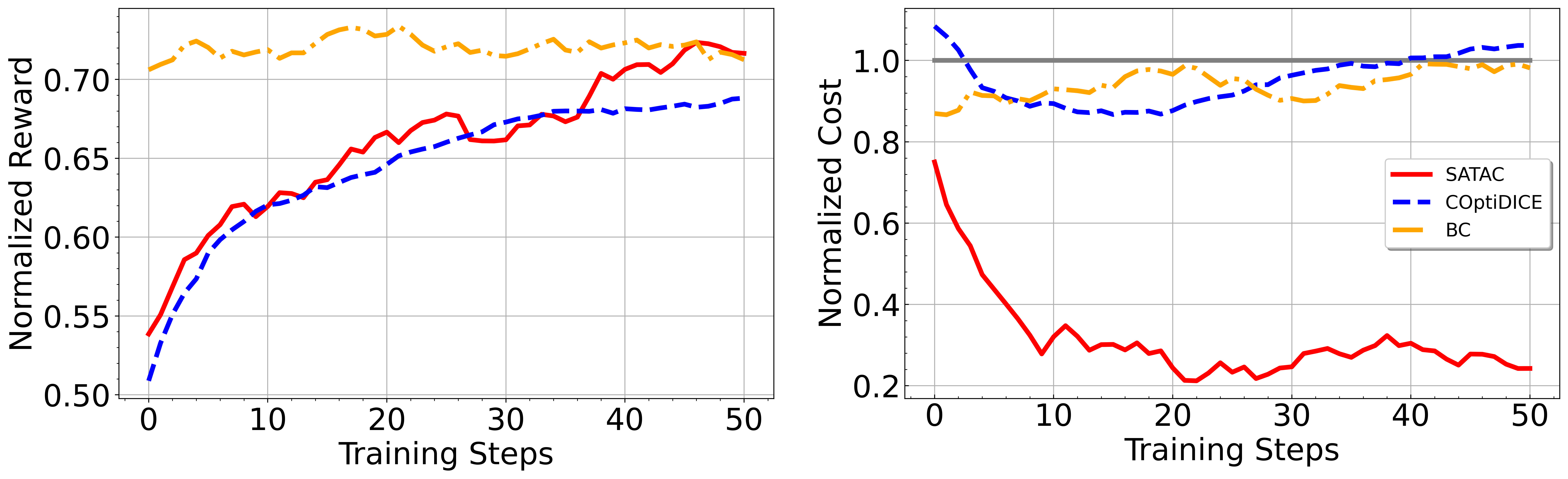
(b) BallCircle

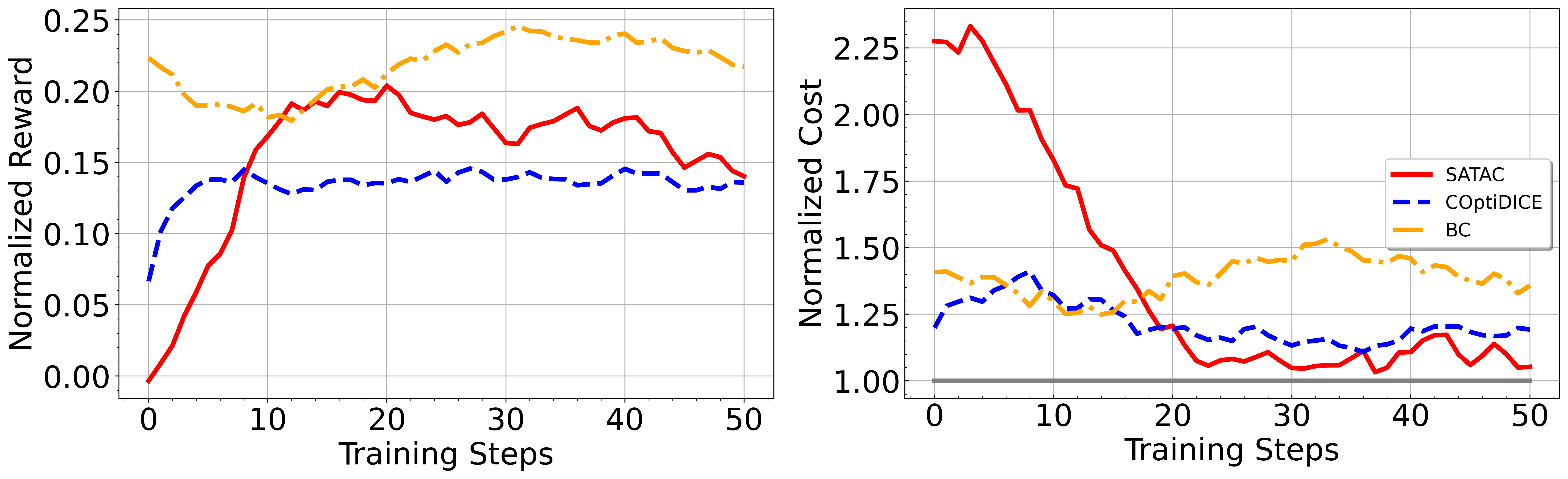
(c) PointButton

Figure 4: Evaluation results during training (each value is the moving average over $20$ evaluation episodes and $3$ random seeds, and the cost threshold is $1$ (any normalized cost below $1$ is considered as safe).

C.4 Experimental settings

We run all the experiments with NVIDIA GeForce RTX $3080$ Ti $8-$Core Processor.

References

• Achiam et al., (2017) Achiam, J., Held, D., Tamar, A., and Abbeel, P. (2017). Constrained policy optimization. In Int. Conf. Machine Learning (ICML), volume 70, pages 22–31. JMLR.
• Agarwal et al., (2021) Agarwal, A., Kakade, S. M., Lee, J. D., and Mahajan, G. (2021). On the theory of policy gradient methods: Optimality, approximation, and distribution shift. Journal of Machine Learning Research, 22(98):1–76.
• Antos et al., (2008) Antos, A., Szepesvári, C., and Munos, R. (2008). Learning near-optimal policies with bellman-residual minimization based fitted policy iteration and a single sample path. Machine Learning, 71:89–129.
• Bertsekas and Tsitsiklis, (1996) Bertsekas, D. and Tsitsiklis, J. N. (1996). Neuro Dynamic Programming. Athena Scientific.
• Boyd and Vandenberghe, (2004) Boyd, S. and Vandenberghe, L. (2004). Convex Optimization. Cambridge Univ. Press, New York, NY.
• Brantley et al., (2020) Brantley, K., Dudik, M., Lykouris, T., Miryoosefi, S., Simchowitz, M., Slivkins, A., and Sun, W. (2020). Constrained episodic reinforcement learning in concave-convex and knapsack settings. In Advances Neural Information Processing Systems (NeurIPS), volume 33, pages 16315–16326. Curran Associates, Inc.
• Bura et al., (2021) Bura, A., HasanzadeZonuzy, A., Kalathil, D., Shakkottai, S., and Chamberland, J.-F. (2021). Safe exploration for constrained reinforcement learning with provable guarantees. arXiv preprint arXiv:2112.00885.
• (8) Chen, F., Zhang, J., and Wen, Z. (2022a). A near-optimal primal-dual method for off-policy learning in cmdp. In Advances Neural Information Processing Systems (NeurIPS), volume 35, pages 10521–10532.
• Chen and Jiang, (2019) Chen, J. and Jiang, N. (2019). Information-theoretic considerations in batch reinforcement learning. In Int. Conf. Machine Learning (ICML), pages 1042–1051. PMLR.
• (10) Chen, L., Jain, R., and Luo, H. (2022b). Learning infinite-horizon average-reward markov decision process with constraints. In Int. Conf. Machine Learning (ICML), pages 3246–3270. PMLR.
• Cheng et al., (2020) Cheng, C.-A., Kolobov, A., and Agarwal, A. (2020). Policy improvement via imitation of multiple oracles. In Advances Neural Information Processing Systems (NeurIPS), volume 33, pages 5587–5598.
• Cheng et al., (2022) Cheng, C.-A., Xie, T., Jiang, N., and Agarwal, A. (2022). Adversarially trained actor critic for offline reinforcement learning. In International Conference on Machine Learning, pages 3852–3878. PMLR.
• Chow et al., (2017) Chow, Y., Ghavamzadeh, M., Janson, L., and Pavone, M. (2017). Risk-constrained reinforcement learning with percentile risk criteria. The Journal of Machine Learning Research, 18(1):6070–6120.
• Ding et al., (2021) Ding, D., Wei, X., Yang, Z., Wang, Z., and Jovanovic, M. (2021). Provably efficient safe exploration via primal-dual policy optimization. In Int. Conf. Artificial Intelligence and Statistics (AISTATS), volume 130, pages 3304–3312. PMLR.
• Ding and Lavaei, (2022) Ding, Y. and Lavaei, J. (2022). Provably efficient primal-dual reinforcement learning for cmdps with non-stationary objectives and constraints. arXiv preprint arXiv:2201.11965.
• (16) Efroni, Y., Mannor, S., and Pirotta, M. (2020a). Exploration-exploitation in constrained MDPs. arXiv preprint arXiv:2003.02189.
• (17) Efroni, Y., Mannor, S., and Pirotta, M. (2020b). Exploration-exploitation in constrained mdps. arXiv preprint arXiv:2003.02189.
• Fan et al., (2020) Fan, J., Wang, Z., Xie, Y., and Yang, Z. (2020). A theoretical analysis of deep q-learning. In Learning for Dynamics and Control, pages 486–489. PMLR.
• Farahmand et al., (2010) Farahmand, A.-m., Szepesvári, C., and Munos, R. (2010). Error propagation for approximate policy and value iteration. Advances in Neural Information Processing Systems, 23.
• Fujimoto and Gu, (2021) Fujimoto, S. and Gu, S. S. (2021). A minimalist approach to offline reinforcement learning. Advances in neural information processing systems, 34:20132–20145.
• Fujimoto et al., (2019) Fujimoto, S., Meger, D., and Precup, D. (2019). Off-policy deep reinforcement learning without exploration. In International conference on machine learning, pages 2052–2062. PMLR.
• Fujimoto et al., (2018) Fujimoto, S., van Hoof, H., and Meger, D. (2018). Addressing function approximation error in actor-critic methods. In Int. Conf. Machine Learning (ICML), pages 1582–1591.
• Guo et al., (2023) Guo, H., Qi, Z., and Liu, X. (2023). Rectified pessimistic-optimistic learning for stochastic continuum-armed bandit with constraints. In Learning for Dynamics and Control Conference, pages 1333–1344. PMLR.
• Haarnoja et al., (2018) Haarnoja, T., Zhou, A., Abbeel, P., and Levine, S. (2018). Soft Actor-Critic: Off-policy maximum entropy deep reinforcement learning with a stochastic actor. In Int. Conf. Machine Learning (ICML), pages 1861–1870.
• Hong et al., (2023) Hong, K., Li, Y., and Tewari, A. (2023). A primal-dual-critic algorithm for offline constrained reinforcement learning. arXiv preprint arXiv:2306.07818.
• Isele et al., (2018) Isele, D., Nakhaei, A., and Fujimura, K. (2018). Safe reinforcement learning on autonomous vehicles. In 2018 IEEE/RSJ International Conference on Intelligent Robots and Systems (IROS), pages 1–6. IEEE.
• Ji et al., (2023) Ji, J., Zhang, B., Pan, X., Zhou, J., Dai, J., and Yang, Y. (2023). Safety-gymnasium. GitHub repository.
• Jin et al., (2020) Jin, C., Yang, Z., Wang, Z., and Jordan, M. I. (2020). Provably efficient reinforcement learning with linear function approximation. In Conference on Learning Theory, pages 2137–2143. PMLR.
• Jin et al., (2021) Jin, Y., Yang, Z., and Wang, Z. (2021). Is pessimism provably efficient for offline rl? In International Conference on Machine Learning, pages 5084–5096. PMLR.
• Kakade and Langford, (2002) Kakade, S. and Langford, J. (2002). Approximately optimal approximate reinforcement learning. In Int. Conf. Machine Learning (ICML), pages 267–274.
• Kakade, (2001) Kakade, S. M. (2001). A natural policy gradient. In Advances Neural Information Processing Systems (NeurIPS).
• Kidambi et al., (2020) Kidambi, R., Rajeswaran, A., Netrapalli, P., and Joachims, T. (2020). Morel: Model-based offline reinforcement learning. Advances in neural information processing systems, 33:21810–21823.
• Kingma and Ba, (2015) Kingma, D. P. and Ba, J. (2015). Adam: A method for stochastic optimization. In Bengio, Y. and LeCun, Y., editors, Int. Conf. on Learning Representations (ICLR).
• Konda and Tsitsiklis, (2000) Konda, V. and Tsitsiklis, J. (2000). Actor-critic algorithms. In Solla, S., Leen, T., and Müller, K., editors, Advances in Neural Information Processing Systems, volume 12. MIT Press.
• Kumar et al., (2019) Kumar, A., Fu, J., Soh, M., Tucker, G., and Levine, S. (2019). Stabilizing off-policy q-learning via bootstrapping error reduction. Advances in Neural Information Processing Systems, 32.
• Laroche et al., (2019) Laroche, R., Trichelair, P., and Des Combes, R. T. (2019). Safe policy improvement with baseline bootstrapping. In International conference on machine learning, pages 3652–3661. PMLR.
• Lattimore and Szepesvári, (2020) Lattimore, T. and Szepesvári, C. (2020). Bandit Algorithms. Cambridge University Press.
• Lee et al., (2021) Lee, J., Jeon, W., Lee, B., Pineau, J., and Kim, K.-E. (2021). Optidice: Offline policy optimization via stationary distribution correction estimation. In Meila, M. and Zhang, T., editors, Int. Conf. Machine Learning (ICML), volume 139 of Proceedings of Machine Learning Research, pages 6120–6130. PMLR.
• Liu et al., (2021) Liu, T., Zhou, R., Kalathil, D., Kumar, P., and Tian, C. (2021). Learning policies with zero or bounded constraint violation for constrained MDPs. In Advances Neural Information Processing Systems (NeurIPS), volume 34.
• Liu et al., (2020) Liu, Y., Swaminathan, A., Agarwal, A., and Brunskill, E. (2020). Provably good batch off-policy reinforcement learning without great exploration. Advances in neural information processing systems, 33:1264–1274.
• Liu et al., (2023) Liu, Z., Guo, Z., Lin, H., Yao, Y., Zhu, J., Cen, Z., Hu, H., Yu, W., Zhang, T., Tan, J., et al. (2023). Datasets and benchmarks for offline safe reinforcement learning. arXiv preprint arXiv:2306.09303.
• Munos and Szepesvári, (2008) Munos, R. and Szepesvári, C. (2008). Finite-time bounds for fitted value iteration. Journal of Machine Learning Research, 9(5).
• Paine et al., (2020) Paine, T. L., Paduraru, C., Michi, A., Gulcehre, C., Zolna, K., Novikov, A., Wang, Z., and de Freitas, N. (2020). Hyperparameter selection for offline reinforcement learning. arXiv preprint arXiv:2007.09055.
• Pirotta et al., (2013) Pirotta, M., Restelli, M., Pecorino, A., and Calandriello, D. (2013). Safe policy iteration. In Int. Conf. Machine Learning (ICML), pages 307–315. PMLR.
• Rashidinejad et al., (2021) Rashidinejad, P., Zhu, B., Ma, C., Jiao, J., and Russell, S. (2021). Bridging offline reinforcement learning and imitation learning: A tale of pessimism. In Advances Neural Information Processing Systems (NeurIPS), volume 34, pages 11702–11716.
• Singh et al., (2020) Singh, R., Gupta, A., and Shroff, N. B. (2020). Learning in markov decision processes under constraints. arXiv preprint arXiv:2002.12435.
• Tittaferrante and Yassine, (2022) Tittaferrante, A. and Yassine, A. (2022). Hyperparameter tuning in offline reinforcement learning. In 2022 21st IEEE International Conference on Machine Learning and Applications (ICMLA), pages 585–590.
• Von Stackelberg, (2010) Von Stackelberg, H. (2010). Market structure and equilibrium. Springer Science & Business Media.
• Wei et al., (2023) Wei, H., Ghosh, A., Shroff, N., Ying, L., and Zhou, X. (2023). Provably efficient model-free algorithms for non-stationary CMDPs. In Int. Conf. Artificial Intelligence and Statistics (AISTATS), pages 6527–6570. PMLR.
• (50) Wei, H., Liu, X., and Ying, L. (2022a). A provably-efficient model-free algorithm for infinite-horizon average-reward constrained markov decision processes. In AAAI Conf. Artificial Intelligence.
• (51) Wei, H., Liu, X., and Ying, L. (2022b). Triple-Q: a model-free algorithm for constrained reinforcement learning with sublinear regret and zero constraint violation. In Int. Conf. Artificial Intelligence and Statistics (AISTATS).
• Wu et al., (2021) Wu, R., Zhang, Y., Yang, Z., and Wang, Z. (2021). Offline constrained multi-objective reinforcement learning via pessimistic dual value iteration. In Advances Neural Information Processing Systems (NeurIPS), volume 34, pages 25439–25451.
• Xie et al., (2021) Xie, T., Cheng, C.-A., Jiang, N., Mineiro, P., and Agarwal, A. (2021). Bellman-consistent pessimism for offline reinforcement learning. Advances in neural information processing systems, 34:6683–6694.
• Xie and Jiang, (2020) Xie, T. and Jiang, N. (2020). Q* approximation schemes for batch reinforcement learning: A theoretical comparison. In Conference on Uncertainty in Artificial Intelligence, pages 550–559. PMLR.
• Xu et al., (2022) Xu, H., Zhan, X., and Zhu, X. (2022). Constraints penalized q-learning for safe offline reinforcement learning. In AAAI Conf. Artificial Intelligence, volume 36, pages 8753–8760.
• Yu et al., (2020) Yu, T., Thomas, G., Yu, L., Ermon, S., Zou, J. Y., Levine, S., Finn, C., and Ma, T. (2020). Mopo: Model-based offline policy optimization. Advances Neural Information Processing Systems (NeurIPS), 33:14129–14142.
• Zanette et al., (2021) Zanette, A., Wainwright, M. J., and Brunskill, E. (2021). Provable benefits of actor-critic methods for offline reinforcement learning. Advances in neural information processing systems, 34:13626–13640.
• Zhang and Jiang, (2021) Zhang, S. and Jiang, N. (2021). Towards hyperparameter-free policy selection for offline reinforcement learning. Advances Neural Information Processing Systems (NeurIPS), 34:12864–12875.
• Zhu et al., (2023) Zhu, H., Rashidinejad, P., and Jiao, J. (2023). Importance weighted actor-critic for optimal conservative offline reinforcement learning. arXiv preprint arXiv:2301.12714.