Decision Making under Costly Sequential Information Acquisition:
the Paradigm of Reversible and Irreversible Decisions

Abstract

Decision making in modern stochastic systems, including e-commerce platforms, financial markets, and healthcare systems, has evolved into a multifaceted process that involves information acquisition and adaptive information sources. This paper initiates a study on this integrated process, where these elements are not only fundamental but also interact in a complex and dynamically intertwined manner.

We introduce a relatively simple model, which, however, captures the novel elements we consider. Specifically, a decision maker (DM) can choose between an established product $A$ with a known value and a new product $B$ with an unknown value. The DM can observe signals about the unknown value of product $B$ and can also opt to exchange it for product $A$ if $B$ is initially chosen. Mathematically, the model gives rise to a sequential optimal stopping problem with two different informational regimes (before and after buying product $B$), differentiated by the initial, coarser signal and the subsequent, finer one. We analyze the underlying problems using predominantly viscosity solution techniques, differing from the existing literature on information acquisition which is based on traditional optimal stopping techniques. Additionally, our modeling approach offers a novel framework for developing more complex interactions among decisions, information sources, and information costs through a sequence of nested obstacles.

1 Introduction

The paper initiates a study that integrates costly information acquisition, adaptive information sources, and sequential decision making. The motivation comes from numerous applications in which these elements not only play a fundamental role but also interact and influence each other in a rather complex, dynamic intertwined way.

In medical care, doctors continually adjust treatment plans for chronic conditions such as diabetes, guided by ongoing assessments of patient health and lifestyle changes [37]. However, learning about each patient’s evolving health conditions requires effort and care, and informational sources do not remain static. In finance, investors and fund managers make sequential investment decisions influenced by evolving market trends, economic data, and realized returns while in parallel seeking information from, frequently, distinct sources [10, 11, 12]. Supply chain managers adjust inventory and logistics strategies based on real-time sales trends and consumer demands, while they harvest information from newly coming sources [8, 21]. In retail, consumers routinely return products they use for a short amount of time while, in parallel, learning more about their quality as well as about the price and quality of comparable products [14, 15]. In the context of dynamic contract design, the principal faces the challenge of dynamically monitoring labor activities to minimize adverse event occurrences [5]. These examples underscore the critical importance of information in making informed, adaptive decisions in contexts where complete information is not only unavailable, but its acquisition is costly and, furthermore, it changes regimes and accuracy while decisions are, in parallel, being intertemporally made.

To our knowledge, the literature on models that combine sequential decision making with dynamically changing costly information sources is not adequately developed. Indeed, the existing models predominantly consider both a single information source and a single decision occurring at an (optimal) time, at which the problem immediately terminates. Herein, we aim at relaxing both these features by allowing, from the one hand, distinct costly information sources across time and, from the other, sequential decisions which may even include reversal of previous ones.

Herein, we build a general model motivated mainly from E-commerce. On such platforms, we often encounter situations where a new product of unknown quality is introduced to compete against existing ones of known quality. A buyer who is choosing between this new product and several old products could collect information on the former by reading reviews, and decide whether to purchase it or not. Meanwhile, she could also access information about the pricing of existing products on the platform. As most of the E-commerce platforms offer flexible return and exchange services (especially for new products), buyers could first purchase either the new product or a known, established, one, after a preliminary investigation. If the buyer is unsatisfied with the initial purchase, she can return the product and exchange it with the alternative (possibly with a penalty). Similar decision making problems with learning and opportunity to reverse can also be found in airline and hotel bookings. Frequently, travelers, looking for airline tickets, at first purchase “flexible” tickets (with no or low cancellation fee) after investigating different options. They may then continue collecting information on these options and also checking for updated ticket prices. If a better option arises later, a traveler may pay a fee to cancel the existing ticket and switch to the one she prefers better. Another example, that falls into this framework, is membership subscriptions. Service providing entities, such as gyms and news subscription companies, frequently introduce alternative plans as a strategy to expand their business operations and stimulate increased customer engagement. Existing clients are presented with an option to choose between these new plans and their current subscriptions. Furthermore, there is an opportunity for these clients to revert to their original plan, albeit at a financial cost, after a trial period with the new plan.

We introduce a relatively simple model, which however captures the novel elements we consider. In an infinite horizon setting, a decision maker (DM) may choose between two products, $A$ and $B$. Product $A$ is established and offers a known return. Product $B$, on the other hand, has been only recently introduced, and its actual value is unknown. The latter is modeled as a binomial random variable $\Theta$. While its two values are known to the DM, she learns about $\Theta$ under a noisy signal $Y_{t}$ over a time period before making her initial decision, to buy $A$ or $B$. This noisy signal may be, for example, understood as posted reviews of product $B$ on an E-commerce platform.

If the DM chooses product $B$, she is offered the optionality to return it and switch to product $A$ at a later instant chosen by the user. This optionality is not cost-free as the DM must pay a return fee. On the other hand, she is now able to evaluate product $B$ more accurately through its use and, more broadly, through a new informational signal which is naturally more accurate than the initial one. This updated learning procedure continues either till the DM decides to return the product, pay the return fee, and terminate the problem or indefinitely if the DM decides to keep product $B$. See Figure 1 for the timeline of the decisions. In both cases, learning occurs within a Bayesian framework, as in the classical filtering theory.

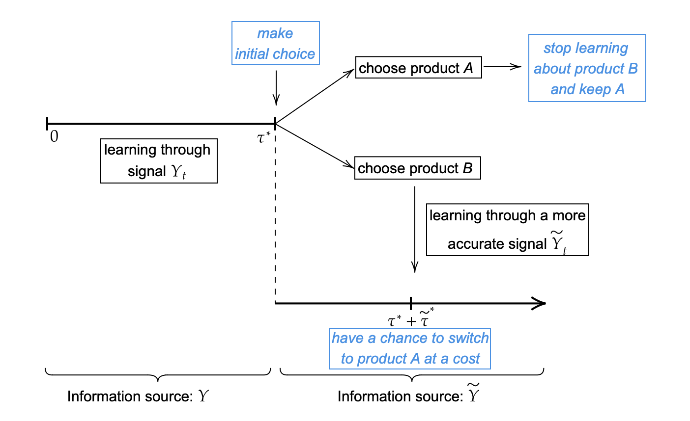
Figure 1: Timeline of the decisions.

Mathematically, the model gives rise to a sequential optimal stopping problem with two different informational regimes, differentiated by the initial, coarser signal and the subsequent, finer one. More precisely, the obstacle term in the “outer” decision making problem is itself a value function of another, “nested”, optimal stopping problem. Each of these two problems corresponds to distinct informational sources, costs, and utility flows and their analysis highlights the complex interactions between decisions, information sources, learning, and the associated payoffs and costs.

We analyze the underlying problems using predominantly viscosity solution techniques, for enough regularity may not be always achieved. Furthermore, viscosity arguments allow for a unified approach to obtain existence, uniqueness, and comparison results. They are also flexible enough to perform sensitivity analysis and to study the limiting behavior of the solutions and the free boundaries, by building suitable sub- and super-solutions. Methodologically, our approach thus differs from existing ones which are based on traditional optimal stopping techniques. As a matter of fact, a special/benchmark case of what we consider is the single decision (irreversible) problem, which has been extensively analyzed; see, for example, [4, 9, 28, 38]. Our approach offers a complementary way to analyze it. We also note that, from a mathematical perspective, the concepts of “reversible” and “irreversible” decisions can be unified under the optimal stopping problem framework we propose but with a general, considerably more complex obstacle. However, the nature of this obstacle differs for each type of decision. The modeling approach herein offers a novel framework for developing more complex interactions among decisions, information sources, and information costs achieved through a sequence of nested obstacles.

Related Literature.

Our work is related to two lines of literature, one on decision making under costly information acquisition and one on stochastic control with filtering.

Decision making under information acquisition has a long history, dating back to the seminal paper [36], in which the flow of information is assumed to be fully exogenous, and the DM only controls the decision time and action choice. Specifically, [36] formulates an optimal stopping problem where the entire space of beliefs can be partitioned into a stopping region and a continuation region. Early works along this direction have focused on the duration of search when there is a cost per unit of time when seeking information. For example, [28] generalizes the framework in [36] to an information intensity control problem where information is modeled as the trajectory of a Brownian motion with the drift representing the state and the variance representing the intensity. [25] characterizes the solution to the dynamic rational inattention problem using the posterior-based approach. [17] tackles the problem of acquiring information on multiple alternatives simultaneously, characterizing a star-shaped optimal stopping boundary and the corresponding value function.

A similar setting is used in [9] to study the trade-off between information speed and precision. Some recent works have been trying to address the information selection issue when there are multiple information sources and when the DM has limited capacity to process information. In this paradigm, [4, 24] study the allocation of limited attention when there are multiple sources of information that are modeled by Poisson bandits. Work [23] has a similar focus and assumes that the DM sequentially samples from a finite set of Gaussian signals and aims to predict a persistent multi-dimensional state at an unknown final period. The authors show that the optimal choice from Gaussian information sources is myopic. Recently, [38] studies a setting where the DM has access to both Gaussian signals (which are available in continuous time but are very noisy) and Poisson signals (which are less frequent but contain precise information). Another tropical area of focus is partially observable Markov decision processes. In this context, [31] investigates the optimal times for acquiring costly observations and determining subsequent optimal action values. In addition, [1] examines a scenario where the DM sequentially evaluates a stream of decision tasks to make optimal choices, exploring the impact of task accumulation and time pressure on her decisions. This framework can also be used to understand the equilibrium of information gathering in which the decisions of the agents affect their speed of access to information [3].

However, despite the importance of addressing the search duration and information selection questions, most of the decisions considered in these papers are rather oversimplified (e.g., a static single decision between two products) or extremely abstract (a general form of the terminal cost with no further analysis). As the decision is an integral part of the framework and has a considerable impact on the learning process and information search behavior, it is crucial to discuss some realistic downstream decision making scenario and examine how these tasks affect learning behavioral patterns. To the best of our knowledge, this aspect has been largely missing in the literature.

In stochastic control literature with filtering, the DM has partial information about the underlying system which is often modeled through a stochastic differential equation (SDE). The DM will first use the observation process to form an estimate of the state of the system and then, thanks to the separation principle [32], construct the control signal as a function of this estimate. For this line of work, the observation process is often assumed to be obtained at no cost. The main focus, on the other hand, is on the construction of the filtering process and the solvability of the associated control problem [26, 33]. Most of the studies have been focused on linear-quadratic problems [2, 27, 34]. This is because a tractable finite dimensional Kalman-Bucy filter can be derived in explicit form when the underlying SDE is linear, and the associated control problem can be, in turn, solved through the Riccati system when the cost function is quadratic. Although sharing some common ingredients with our framework such as using the Bayesian formula to estimate unknown quantities, the partially observed quantities considered in this line of work are often more complex (i.e., unknown processes) than those considered in the literature on information acquisition (i.e., unknown variables). More importantly, the settings considered in stochastic control and filtering theory cannot be applied directly to the situation where the DM pays a cost to process information and to facilitate the understanding of how the cost of information affects the behavior of the DM.

Our Contributions.

Our contribution is twofold, modeling and methodological. We propose a general model that integrates sequential decision making, distinct informational sources, and information acquisition costs. To our knowledge, this is the first model with such features. It gives rise to new kind of optimal stopping problems in which the obstacles themselves solve different, nested, optimal stopping problems. The obstacles take a general form which, in turn, requires a more involved analysis.

Methodologically, we develop a viscosity theory toolkit that allows us to study various aspects of the underlying optimal stopping problems. We also recover, as a special case, the well-known problem with a single (irreversible) decision which we solve with the complementary viscosity techniques. The viscosity theory allows us to perform a rather detailed analysis and study, among others, the effects of the return fee on both decisions of the DM, the behavior of the solution in terms of the volatility of the signals, the width of the exploratory regions in terms of the various modeling parameters, as well as various limiting cases. In particular, we find that i) the return optionality makes the DM spend less effort to explore the value of $\Theta$ during the first decision period, ii) if the exchange fee is comparatively small, the DM makes her first choice earlier compared to the situation when the return cost is high, and iii) if the exchange cost is relatively high, the DM is more willing to choose the well-known product $A$ than choosing the new product $B$.

We finally note that the setting for the “irreversible” decisions part is akin to the set-up in [28], where the precision of the information signal can be further controlled at a cost. However, the mathematical tools used in our framework are markedly different. Work [28] uses the smooth-fit principle to characterize the continuation and stopping regions under the assumption that the value function is twice continuously differentiable. In contrast, we construct proper sub/super viscosity solutions and utilize the comparison principle to identify the continuation and stopping regions, and to establish the asymptotic and monotonicity behavior with respect to the model parameters. Some of the constructions are non-trivial and rather delicate, particularly in the sensitivity analysis. However, the discussion on sensitivity analysis in [28] is limited and, at various points, lacks mathematical details.

The paper is organized as follows. In Section 2, we introduce the new extended model and study the underlying integrated optimal stopping problem. We present the main regularity results, the sensitivity analysis, and the limiting behavior of its solutions and of the free boundaries. We also study the special case of irreversible decisions. In Section 3, we study the general problem for two distinct kinds of information sources after the initial exploratory period. Namely, we study the cases of a Poisson and a Gaussian signal, respectively, and study various questions, among others, about the effects of the return penalty on the optimal decisions of the DM. We conclude in Section 4.

2 The general decision making model under costly sequential information

A DM acts in an environment in which two products, $A$ and $B,$ are available. Product $A$ has known performance modeled by a given constant $\mu>0$ while product $B$ is new, and not yet established. The quality of product $B$ is not entirely known and is modeled by a random variable $\Theta,$ which may take only two possible values, $l$ and $h$. The DM knows these values but not the actual performance of product $B$. For this, she formulates beliefs using informational signals in a Bayesian framework. The signals, however, are costly while they are being used.

In all existing works, the DM starts at time $0,$ chooses a signal process, and pays information acquisition costs while she learns about the new product. At some time, say $\tau\geq 0,$ she chooses one of the two products and the problem terminates. There is a rich literature on this problem and we provide further comments and references in the sequel.

Herein, we depart from the known settings and propose a new, extended model which allows for i) subsequent decision making beyond the initial (decision) time, ii) access to sequentially differential information and iii) reversal of the initial decision at a cost.

Specifically, after her initial choice at time $\tau^{\ast}$, the DM begins using the product she chose while continuing learning about it. The latter is carried out through a new, more accurate refined signal since now the DM has access to the product itself. At some future time $\tau^{\ast}+\widetilde{\tau}^{\ast}$, with $\widetilde{\tau}^{\ast}\leq\infty$, she makes a second choice: either returns the initially chosen product $\left(\widetilde{\tau}^{\ast}<\infty\right)$ and switches to the alternative, or keeps it $\left(\widetilde{\tau}^{\ast}=\infty\right)$, and the problem terminates. To our knowledge, such models have not been considered before.

We describe the new model next. Starting at time $t=0$, the DM chooses a Gaussian signal process, say $Y$, solving

$$dY_{t}=\,\Theta\,dt+\sigma dW_{t},\text{ \ }Y_{0}=0,$$ (2.1)

with $\sigma>0$ and $W$ being a standard Brownian motion in a probability space $\left(\Omega,\mathcal{F},\mathbb{P}\right)$. In turn, she dynamically updates her views, based on the information generated by $Y$, acquiring the belief process $q$ where

$$q_{t}:=\mathbb{P}\left[\left.\Theta=h\right|\mathcal{F}_{t}^{Y}\right],$$ (2.2)

with $\mathcal{F}_{t}^{Y}:=\sigma(Y_{s};0\leq s\leq t)$.

Classical results from filtering theory (see, for example, [16], also [28, 38] and others) yield that $q$ is a martingale, solving

$$dq_{t}=\frac{h-l}{\sigma}q_{t}\left(1-q_{t}\right)dZ_{t},\text{ \ }q_{0}=q\in\left[0,1\right],$$ (2.3)

with $Z$ being a standard Brownian motion in $\left(\Omega,\mathcal{F},\left\{\mathcal{F}_{t}^{Y}\right\},\mathbb{P}\right)$. Note that the states $0$ and $1$ are absorbing, i.e. if the initial belief $q_{0}=0,1$ then $q_{t}=0,1$, for $t>0$, respectively.

To have access to this signal process, the DM encounters information acquisition cost. It is assumed that they occur at a discounted rate $C(q)$ per unit of time, namely, the process (with a slight abuse of notation)

$$C_{t}:=\int_{0}^{t}e^{-\rho s}C(q_{s})ds,\text{ \ \ }\rho>0,$$ (2.4)

is the cumulative cost of acquiring information in $\left[0,t\right]$ through signal $Y$. It is assumed that there are neither initial fixed costs nor cost jumps thereafter.

Examples: i)  $C(q)=C_{I}>0.$ This constant cost case has been extensively studied (see, [19, 20]). We also study it herein but in a more general context. In this case, the cumulative information cost is deterministic with $C_{t}=\left(1-e^{-\rho t}\right)\frac{C_{I}}{\rho}$.

ii) $C\left(q\right)=\operatorname{Var}\left[\left.\Theta\right|q\right]$ (or $C\left(q\right)=\sqrt{\operatorname{Var}\left[\left.\Theta\right|q\right]}).$ The cumulative information cost is stochastic, $C_{t}=\int_{0}^{t}e^{-\rho s}\operatorname{Var}\left[\left.\Theta\right|q_{s}\right]ds$ (or $C_{t}=\int_{0}^{t}e^{-\rho s}\sqrt{\operatorname{Var}\left[\left.\Theta\right|q_{s}\right]}ds)$, and relates to the uncertainty in the DM’s belief through time.

The DM acts under the belief process $q$ till time $\tau^{\ast}$ at which she makes her initial choice. Right afterward, a new signal is activated related to a different process $\widetilde{Y}$, which generates its own belief process $\widetilde{q}$. In any upcoming interval $\left[\tau^{\ast},\tau^{\ast}+\widetilde{\tau}\right],$ she receives utility from the product she acquired at time $\tau^{\ast}$ while she refines her knowledge about it. Then, at an optimal time $\tau^{\ast}+\widetilde{\tau}^{\ast}$ she decides whether to return it and exchange it with the other product, or keep it (i.e. $\widetilde{\tau}^{\ast}=\infty)$. The problem then terminates.

The value function of the DM, $V:\left[0,1\right]\rightarrow\mathbb{R},$ is defined as

$$V(q)=\sup_{\tau\in\mathcal{T}_{Y}}\mathbb{E}\left.\left[-\int_{0}^{\tau}e^{-\rho t}C(q_{t})dt+e^{-\rho\tau}{G(q}_{\tau}{)}\right|q_{0}=q\right],$$ (2.5)

where $\mathcal{T}_{Y}$ is the set of stopping times generated by the signal process $Y$,

$$\mathcal{T}_{Y}:=\left\{\tau\geq 0,\text{ }\tau\in\left\{\mathcal{F}_{t}^{Y}\right\}\right\}.$$ (2.6)

The function $G:\left[0,1\right]\rightarrow\mathbb{R}$ is modeled as

$$G(q)=\max\Big{(}V_{A}(q),V_{B}(q)\Big{)}$$ (2.7)

where $V_{A}(q)$ and $V_{B}(q)$ represent the rewards the DM will receive at times beyond the instant she makes her initial choice. The subscripts $A$ and $B$ correspond to the products initially chosen by the DM. The DM will evaluate the expected payoff $G$ and select the greater of the two rewards, $V_{A}$ or $V_{B}$. We will discuss a few different scenarios of $V_{A}$ and $V_{B}$ in the sequel.

2.1 The single (irreversible) decision model

This is the case that has been so far studied. The problem terminates at the optimal time (when the initial decision is made) in (2.5) and the rewards are, in most works, given by

$$V_{A}\left(q\right)=\mu\text{ \ \ and \ \ }V_{B}(q)=qh+(1-q)l,$$

(see [19, 28, 38]). In other words, the payoff $G$ is the maximum of the known return $\mu$ of product $A$ and the expected return $qh+(1-q)l$ of product $B$ under belief $q$. The DM’s value function takes the form

$$V(q)=\sup_{\tau\in\mathcal{T}_{Y}}\mathbb{E}\left.\left[-\int_{0}^{\tau}e^{-\rho t}C(q_{t})dt+e^{-\rho\tau}\max\Big{(}\mu,q_{\tau}h+(1-q_{\tau})l\Big{)}\right|q_{0}=q\right].$$ (2.8)

A popular case is when the information cost has a constant rate, $C(q)=C_{I}>0,$ $q\in\left[0,1\right].$ This value function,

$$w(q):=\sup_{\tau\in\mathcal{T}_{Y}}\mathbb{E}\left.\left[-\int_{0}^{\tau}e^{-\rho t}C_{I}dt+e^{-\rho\tau}\max\left(\mu,q_{\tau}h+(1-q_{\tau})l\right)\right|q_{0}=q\right],$$ (2.9)

will serve as a benchmark quantity in the sequel.

2.2 The extended (reversible) decision model

We introduce a general decision making model with costly information acquisition and differential informational signals. Specifically, after her initial decision (between $A$ or $B)$, the DM starts using the chosen product, explores it and continues learning about it. For generality, we assume that, even at this stage, complete information about the product is not entirely accessible but, instead, the new informational signal is more accurate than the initial one. The DM has the optionality to return the product at a cost and replace it with the other one, and then the problem terminates. Otherwise, she retains the product that was chosen initially.

To keep the analysis tractable, we assume that the known product $A$ is not returnable so the optionality to reverse the initial choice is available only if the DM first chooses the unknown product $B.$ This is done only for convenience as, mathematically, the analysis is the same, albeit more involved.

If the DM chooses product $B$ at $\tau^{\ast}$, she continues learning about it via a new signal process $\widetilde{Y}_{t}$, which, in analogy to (2.1), generates a new belief process, $\widetilde{q}_{t}$ (see, (3.5) and (3.22)). The DM may decide to keep $B$ or exchange it for $A$, say at time $\tau^{\ast}+\widetilde{\tau}^{\ast}.$ If she returns it, she encounters a return penalty $R(\widetilde{q}_{\widetilde{\tau}^{\ast}})$ and the overall decision process terminates. The form of $R(.)$ is known to the DM at the initial time $0$.

In summary, if she chooses product $B$ at time $\tau^{\ast}$, a new optimization problem is being generated on $\left[\tau^{\ast},\infty\right)$ that incorporates the optionality of exchange, the return penalty and the information acquisition under the new signal. Then, the related value function is given by

$$U_{B}(q_{\tau^{\ast}})\ :={\sup_{\widetilde{\tau}\in\mathcal{T}_{\widetilde{Y}}}}\,\mathbb{\widetilde{E}}\left[\left.\int_{0}^{\widetilde{\tau}}e^{-\rho t}\left(-\widetilde{C}\left(\widetilde{q}_{t}\right)+\widetilde{m}\left(\widetilde{q}_{t}\right))\right)dt+e^{-\rho\widetilde{\tau}}\left(\mu-R(\widetilde{q}_{\widetilde{\tau}})\right)\right|\widetilde{q}_{0}=q_{\tau^{\ast}}\right].$$ (2.10)

Herein, $\widetilde{C}\left(\widetilde{q}\right)$ is the information acquisition cost function for the refined signal $\widetilde{Y}$ and $\widetilde{m}(\widetilde{q})$ the payoff the DM accumulates from using product $B$ in $\left[\tau^{\ast},\tau^{\ast}+\widetilde{\tau}\right]$; for simplicity, we take $\widetilde{C}\equiv 0$. Furthermore, in analogy to (2.6), $\mathcal{T}_{\widetilde{Y}}$ is the set of stopping times associated with the new filtration generated by the modified signal process. We make this all precise in Section 4.

We now formulate the integrated optimization problem in $\left[0,\infty\right]$,

$$V(q)=\sup_{\tau\in\mathcal{T}_{Y}}\mathbb{E}\left.\left[-\int_{0}^{\tau}e^{-\rho t}C(q_{t})dt+e^{-\rho\tau}\max\left(\mu,U_{B}(q_{\tau})\right)\right|q_{0}=q\right].$$ (2.11)

In other words, for the payoff in (2.7) we choose

$$V_{A}\left(q\right)=\mu\text{ \ and \ }V_{B}\left(q\right)=U_{B}\left(q\right),$$

with $U_{B}$ defined in (2.10).

2.3 General regularity results and sensitivity analysis

Whether the DM chooses to work with the irreversible or the reversible decision making problems, the mathematical analysis concerns optimal stopping problems of the general form

$$V(q)=\sup_{\tau\in\mathcal{T}_{Y}}\mathbb{E}\left.\left[-\int_{0}^{\tau}e^{-\rho t}C(q_{t})dt+e^{-\rho\tau}{G(q}_{\tau}{)}\right|q_{0}=q\right],\text{ \ }q\in\left[0,1\right],$$ (2.12)

with the belief process $q$ solving (cf. (2.3)),

$$dq_{t}=\frac{h-l}{\sigma}q_{t}\left(1-q_{t}\right)dZ_{t},\text{ \ }q_{0}=q\in\left[0,1\right],$$

for general information costs and payoff functions $C(.)$ and $G(.),$ respectively.

As mentioned earlier, only the case $(C(q),G(q))=(C_{I}$, ${\max(\mu,qh+(1-q)l))}$ have been so far analyzed; we refer the reader to [19].

Herein, we provide an extended mathematical analysis of (2.11) for general pairs ($C,G)$ under the following mild conditions.

Assumption 1.

1. The information cost $C:[0,1]\rightarrow\mathbb{R}_{+}$ is Lipschitz with Lipschitz constant $L>0$, and for some $C_{1},C_{2},$ $0<C_{1}\leq C(q)\leq C_{2},$ $q\in\left[0,1\right].$

2. The payoff function $G:[0,1]\rightarrow\mathbb{R}_{+}$ is Lipschitz with Lipschitz constant $K>0$, convex and non-decreasing.

3. The model parameters satisfy

   $$0<l<\mu<h\text{ \ \ \ and \ }\sigma>0.$$ (2.13)

Classical results in optimal stopping yield that $V\$is expected to satisfy the variational inequality

$$({\rm OP})\text{ }\left\{\begin{array}[]{c}{\min}\left(\rho V(q)-\frac{1}{2}\left(\frac{h-l}{\sigma}\right)^{2}q^{2}(1-q)^{2}V^{\prime\prime}\left(q\right)+C(q),\,\,V(q)-G(q)\right)=0,\text{ \ \ }q\in\left[0,1\right],\\ \\ V\left(0\right)=G\left(0\right)\text{ \ \ and \ \ }V\left(1\right)=G\left(1\right).\end{array}\right.$$ (2.14)

For the boundary conditions, we recall that $q=0$ is an absorbing state and, thus, (2.12) gives

$$V(0)=\sup_{\tau\in\mathcal{T}}\mathbb{E}\left.\left[-\int_{0}^{\tau}e^{-\rho t}C(0)dt+e^{-\rho\tau}{G(0)}\right|q_{0}=0\right].$$

Using that $C(q)>0$ and $\rho>0,$ we deduce that the optimal time must be $\tau^{\ast}=0$ and $V(0)=G(0)$ follows. Similar arguments yield that $V(1)=G(1)$.

For the reader’s convenience, we highlight below the key steps for the derivation of (2.14). If $q\in\left(0,1\right),$ there are two admissible, in general suboptimal, policies: i) the DM may immediately choose product $A$ or $B,$ without seeking any information about the latter or ii) she may spend some time, say $\left(0,\varepsilon\right]$ with $\varepsilon$ small, learning about $B$ before deciding which product to choose. Choices (i) and (ii) give, respectfully,

$$V(q)\geq G(q),$$ (2.15)

and

$$V(q)\geq\mathbb{E}\left[\left.-\int_{0}^{\varepsilon}e^{-\rho t}C(q_{t})dt+e^{-\rho\varepsilon}V(q_{\varepsilon})\right|q_{0}=q\right].$$

Assuming that $V$ is smooth enough, Itô’s formula gives

$$V(q_{\varepsilon})=V(q)+\int_{0}^{\varepsilon}\frac{1}{2}\left(\frac{h-l}{\sigma}\right)^{2}q_{t}^{2}(1-q_{t})^{2}V^{\prime\prime}\left(q_{t}\right)dt+\int_{0}^{\varepsilon}\sigma V^{\prime}\left(q_{t}\right)dZ_{t},$$

where we used (2.3). Diving by $\varepsilon$ and passing to the limit $\varepsilon\downarrow 0,$ we deduce that

$$\rho V(q)-\frac{1}{2}\left(\frac{h-l}{\sigma}\right)^{2}q^{2}(1-q)^{2}V^{\prime\prime}\left(q\right)+C(q)\geq 0.$$ (2.16)

Because one of these two choices must be optimal, (2.15) or (2.16) must hold as equality and (2.14) follows.

Lemma 1.

There exists a positive constant $\bar{\rho}>0$ such that for $\rho\geq\bar{\rho}$, the value function $V$ is Lipschitz continuous on $\left[0,1\right]$.

Proof.

We show that there exists a positive constant $\rho_{0}=\rho_{0}($$h,l,\sigma)$ such that for $\rho>2\rho_{0}$,

$$|V(q_{1})-V(q_{2})|\leq{\left(\frac{L}{\rho_{0}}+K\right)}|q_{1}-q_{2}|,\text{ \ }q_{1},q_{2}\in[0,1].$$

First note that, for $q_{1},q_{2}\in\left[0,1\right]$, the function $b(q):=\frac{h-l}{\sigma}q(1-q)$ satisfies $b(q)\leq\frac{h-l}{\sigma}q$ and

$$|b(q_{1})-b(q_{2})|\leq\frac{h-l}{\sigma}((1+q_{1}+q_{2})|q_{1}-q_{2}|)\leq 3\frac{h-l}{\sigma}|q_{1}-q_{2}|.$$

Therefore, (see, for example, [29, Theorem 1.3.16]), there exists a positive constant $\rho_{0}=\rho_{0}($$h,l,\sigma)$ such that

$$\mathbb{E}\left[\sup_{0\leq u\leq t}|q_{u}^{q_{1}}-q_{u}^{q_{2}}|\right]\leq e^{\rho_{0}t}|q_{1}-q_{2}|,$$

where $q_{u}^{q_{i}}$ follows the belief process (2.3) with initial state $q_{i}$, $i=1,2$. For $\rho>2\rho_{0}$, we can, similarly, prove that $\mathbb{E}\left[\sup_{t\geq 0}e^{-\rho t}|q_{t}^{q_{1}}-q_{t}^{q_{2}}|\right]\leq|q_{1}-q_{2}|$. In turn, the Lipschitz properties of $C(.)$ and $G(.)$ (see Assumption 1) yield

$$|V(q_{1})-V(q_{2})| \leq {\ \sup_{\tau\in\mathcal{T}_{Y}}}\,\,\mathbb{E}\left[\int_{0}^{\tau}e^{-\rho t}\left|C(q_{t}^{q_{1}})-C(q_{t}^{q_{2}})\right|dt+e^{-\rho\tau}\left|G(q_{\tau}^{q_{1}})-G(q_{\tau}^{q_{2}})\right|\right]$$

$$\leq {\ L}\mathbb{E}\left[\int_{0}^{\infty}e^{-\rho t}\left|q_{t}^{q_{1}}-q_{t}^{q_{2}}\right|dt\right]+{\ K}\mathbb{E}\left[\sup_{t\geq 0}e^{-\rho t}\left|q_{t}^{q_{1}}-q_{t}^{q_{2}}\right|\right]$$

$$\leq {\ \left(\frac{L}{\rho-\rho_{0}}+K\right)}|q_{1}-q_{2}|.$$

∎

The connection between the value function and viscosity solutions of optimal stopping problems was established in [30] (see, also, [29]). Throughout, we will be using viscosity arguments to carry out an extensive analysis of the problem; for completeness, we also highlight the key steps in the following characterization result.

Theorem 2.

The value function $V$ (2.12) is a viscosity solution to (2.14), unique in the class of Lipschitz continuous functions.

Proof.

We first establish that $V$ is a viscosity subsolution of (2.14) in $(0,1).$ For this, let $\bar{q}\in\left(0,1\right)$ and consider a test function $\varphi\in\mathcal{C}^{2}((0,1))$ such that $(V-\varphi)(\bar{q})=\max_{q\in\left(0,1\right)}(V-\varphi)$ and $(V-\varphi)(\bar{q})=0.$ We need to show that

$$\min\left(\rho\varphi\left(\bar{q}\right)-\frac{1}{2}\left(\frac{h-l}{\sigma}\right)^{2}\bar{q}^{2}(1-\bar{q})^{2}\varphi^{\prime\prime}\left(\bar{q}\right)+C(\bar{q}),V(\bar{q})-G(\bar{q})\right)\leq 0.$$

We argue by contradiction, assuming that both inequalities

$$\rho\varphi\left(\bar{q}\right)-\frac{1}{2}\left(\frac{h-l}{\sigma}\right)^{2}\bar{q}^{2}(1-\bar{q})^{2}\varphi^{\prime\prime}\left(\bar{q}\right)+C(\bar{q})>0\text{ \ and \ }V(\bar{q})-G(\bar{q})>0$$ (2.17)

hold. Using the continuity of the involved functions, we obtain that there would exist $\delta>0$ such that, for $0\leq t\leq{\ \hat{\tau}},$

$$\rho\varphi\left(\bar{q}_{t}\right)-\frac{1}{2}\left(\frac{h-l}{\sigma}\right)^{2}\bar{q}_{t}^{2}(1-\bar{q}_{t})^{2}\varphi^{\prime\prime}\left(\bar{q}_{t}\right)+C(\bar{q}_{t})\geq\delta\text{ and }V\left(\bar{q}_{t}\right)-G(\bar{q}_{t})\geq\delta,$$ (2.18)

where $\bar{q}_{t}:=q_{t}^{\bar{q}}{\ }$ denotes the belief process (2.3) with initial state $\bar{q}$ and ${\hat{\tau}}$ is the exit time of $\bar{q}_{t}$ from $[\bar{q}-\delta,\bar{q}+\delta]$.

Applying Itô’s formula to $e^{-\rho t}\varphi(\bar{q}_{t})$, $t\in\left[0,{\hat{\tau}}\wedge\tau\right],$ $\tau\in\mathcal{T}_{Y},$ yields

$$V(\bar{q}) = \varphi(\bar{q})=\mathbb{E}\left[\int_{0}^{{\hat{\tau}}\wedge\tau}e^{-\rho t}(\rho\varphi\left(\bar{q}_{t}\right)-\frac{1}{2}\left(\frac{h-l}{\sigma}\right)^{2}\bar{q}_{t}^{2}(1-\bar{q}_{t})^{2}\varphi^{\prime\prime}\left(\bar{q}_{t}\right))dt+e^{-\rho({\hat{\tau}}\wedge\tau)}\varphi(\bar{q}_{\tau\wedge{\hat{\tau}}})\right]$$

$$\geq \mathbb{E}\left[-\int_{0}^{{\hat{\tau}}\wedge\tau}e^{-\rho t}C(\bar{q}_{t})dt+e^{-\rho\tau}G(\bar{q}_{\tau})\mathbf{1}_{\tau<{\ \hat{\tau}}}+e^{-\rho{\ \hat{\tau}}}V(\bar{q}_{{\ \hat{\tau}}})\mathbf{1}_{{\ \hat{\tau}}\leq\tau}\right]+\delta\mathbb{E}\left[\int_{0}^{{\hat{\tau}}\wedge\tau}e^{-\rho t}dt+e^{-\rho\tau}\mathbf{1}_{\tau<{\hat{\tau}}}\right],$$

where we use that $\varphi\geq V$ on $[\bar{q}-\delta,\bar{q}+\delta]$ and (2.18). Next, we claim that there exists $c_{0}>0$ such that

$$\mathbb{E}\left[\int_{0}^{{\hat{\tau}}\wedge\tau}e^{-\rho t}dt+e^{-\rho\tau}\mathbf{1}_{\tau<{\hat{\tau}}}\right]\geq c_{0},\text{ }\tau\in\mathcal{T}_{Y}.$$

To this end, let $v\left(q\right):=c_{0}\left(1-\frac{1}{\delta^{2}}(q-\bar{q})^{2}\right)$, with $c_{0}=\min\left(\left(\rho+\frac{1}{16}\left(\frac{h-l}{\sigma\delta}\right)^{2}\right)^{-1},1\right)$. Then,

$$\rho v(q)-\frac{1}{2}\left(\frac{h-l}{\sigma}\right)^{2}q^{2}(1-q)^{2}v^{\prime\prime}(q)\leq 1,\text{ \ \ }v(q)\leq c_{0}\leq 1,\text{ \ }q\in(\bar{q}-\delta,\bar{q}+\delta)$$ (2.20)

and

$$v(\bar{q}-\delta)=0\text{, \ }v(\bar{q}+\delta)=0\text{ \ and \ }v(\bar{q})=c_{0}>0.$$ (2.21)

Applying Itô’s formula to $e^{-\rho t}w(\bar{q}_{t})$ gives

$$0<c_{0}=v(\bar{q}) = \mathbb{E}\left[\int_{0}^{{\ \hat{\tau}}\wedge\tau}e^{-\rho t}\left(\rho v\left(\bar{q}_{t}\right)-\frac{1}{2}\left(\frac{h-l}{\sigma}\right)^{2}\bar{q}_{t}^{2}(1-\bar{q}_{t})^{2}v^{\prime\prime}(\bar{q}_{t})\right)dt+e^{-\rho({\ \hat{\tau}}\wedge\tau)}v(\bar{q}_{{\ \hat{\tau}}\wedge\tau})\right]$$ (2.22)

$$\leq \mathbb{E}\left[\int_{0}^{{\ \hat{\tau}}\wedge\tau}e^{-\rho t}dt+e^{-\rho\tau}\mathbf{1}_{\tau<{\ \hat{\tau}}}\right],\text{ }\tau\in\mathcal{T},$$

where the last inequality holds from (2.20) and (2.21). Plugging the last inequality into (LABEL:eq:V_ine), and taking the supremum over $\tau\in\mathcal{T}_{Y}$, it leads to a contradiction with (2.17) to the Dynamic Programing Principle (cf. (2.28)). The supersolution property follows easily and the boundary conditions were justified earlier. For the uniqueness, we refer the reader to [6, Theorem 3.3]. ∎

Next, we study problem (2.12) for general $C(.)$ and obstacle $G$ given by (2.24) below. To our knowledge, only the constant case $C(q)=C_{I},\ q\in[0,1]$ has been so far analyzed in the literature (see [28]).

2.3.1 The exploration and the product-selection regions for general information acquisition costs

We introduce the sets

$$\mathcal{S}:=\left\{\left.q\in[0,1]\,\right|\,\,V(q)=G(q)\right\}\text{ \ and \ }\mathcal{E}:=\left\{\left.q\in[0,1]\right|\,V(q)>G(q)\right\}$$ (2.23)

with

$$G(q)={\max\Big{(}\mu,qh+(1-q)l\Big{)}.}$$ (2.24)

We will refer to $\mathcal{S}$ as the product-selection, or stopping, region since it is therein optimal to immediately stop and choose one of the products. Its complement $\mathcal{E}$ is the continuation region, as it is optimal in this region to keep exploring, and acquiring information about the unknown product. We explore the structure of $\mathcal{S}$ and $\mathcal{E},$ and investigate their dependence on the model parameters.

The analysis is carried out using appropriate sub- and super-viscosity solutions. In Proposition 3 we use the comparison principle. Thus an analytic interpretation of the continuation region $\mathcal{E}$ will be justified in Proposition 4. Several properties of the solution $V$ to the HJB equation (2.14) in this case will be discussed in Theorem 5. We introduce the point $\hat{p}\in(0,1)$,

$$\hat{p}:=\frac{\mu-l}{h-l},$$ (2.25)

which we will use frequently later on. Note that at this point, $G(\hat{p})=\hat{p}h+(1-\hat{p})l=\mu$.

Proposition 3.

The regions $\mathcal{S}$ (stopping) and $\mathcal{E}$ (exploration) are non-empty.

Proof.

i) The region $\mathcal{S}\neq\emptyset$.

We show that there exists a continuous viscosity supersolution $v$, such that $v=G$ in $[0,\varepsilon]\cup[1-\varepsilon,1],$ for sufficiently small $\varepsilon>0$. To this end, for some $M>0$ and $\varepsilon>0$ to be determined, let

$$v(q):=\begin{cases}\mu+M\left(\frac{q}{\varepsilon}-1\right)_{+}^{3},\text{ \ }&0\leq q\leq 2\varepsilon,\\ \mu+M+\frac{q-2\varepsilon}{1-4\varepsilon}(h(1-2\varepsilon)+2l\varepsilon-\mu),\text{ \ }&2\varepsilon\leq q\leq 1-2\varepsilon,\\ qh+(1-q)l+M\left(\frac{1-q}{\varepsilon}-1\right)_{+}^{3},\text{ \ }&1-2\varepsilon\leq q\leq 1.\end{cases}$$

Note that, by construction, $v$ is continuous and twice differentiable at $q=\varepsilon$ and $q=1-\varepsilon$. Furthermore,

$$v^{\prime}(q)=3\frac{M}{\varepsilon}\left(\frac{q}{\varepsilon}-1\right)_{+}^{2}\text{ \ and \ }v^{\prime\prime}(q)=6\frac{M}{\varepsilon^{2}}\left(\frac{q}{\varepsilon}-1\right)_{+},\text{\ \ }0<q<2\varepsilon,$$

$$v^{\prime}(q):=\frac{1}{1-4\varepsilon}(h(1-2\varepsilon)+2l\varepsilon-\mu)\text{ \ and }v^{\prime\prime}\left(q\right)=0,\text{ }2\varepsilon<q<1-2\varepsilon,$$

$$v^{\prime}(q):=h-l-3\frac{M}{\varepsilon}\left(\frac{1-q}{\varepsilon}-1\right)_{+}^{2}\text{ \ and \ }6\frac{M}{\varepsilon^{2}}\left(\frac{1-q}{\varepsilon}-1\right)_{+},\text{\ }1-2\varepsilon<q<1.$$

Then, for $q\in(2\varepsilon,1-2\varepsilon)$,

$$\rho v(q)-\frac{1}{2}\left(\frac{h-l}{\sigma}\right)^{2}q^{2}(1-q)^{2}v^{\prime\prime}\left(q\right)+C\left(q\right)=\rho v(q)+C(q)>0,$$

and, for $q\in[0,2\varepsilon)\cup(1-2\varepsilon,1]$,

$$\rho v(q)-\frac{1}{2}\left(\frac{h-l}{\sigma}\right)^{2}q^{2}(1-q)^{2}v^{\prime\prime}\left(q\right)+C\left(q\right)\geq\rho\mu-6\frac{M}{2\varepsilon^{2}}\left(\frac{h-l}{\sigma}\right)^{2}(2\varepsilon)^{2}\geq\rho\mu-12M\left(\frac{h-l}{\sigma}\right)^{2}.$$

Setting $M:=\frac{\rho\mu}{24}\left(\frac{\sigma}{h-l}\right)^{2}$ the right hand side of the above inequality is positive.

Next, note that $v_{-}^{\prime}(2\varepsilon)=3M\varepsilon^{-1}$ and $v_{+}^{\prime}(1-2\varepsilon)=-3M\varepsilon^{-1}+h-l$. Therefore, by choosing $\varepsilon<\min\left(\frac{3M}{2(\mu-l)},\frac{3M}{2(h-\mu)},\frac{1}{8}\right)$, it holds that

$$v_{-}^{\prime}(2\varepsilon)>\left.\left(\mu+M+\frac{q-2\varepsilon}{1-4\varepsilon}(h(1-2\varepsilon)+2l\varepsilon-\mu)\right)_{+}^{\prime}\right|_{q=2\varepsilon}$$

$$=\left.\left(\mu+M+\frac{q-2\varepsilon}{1-4\varepsilon}(h(1-2\varepsilon)+2l\varepsilon-\mu)\right)_{-}^{\prime}\right|_{q=1-2\varepsilon}$$

$$=\frac{h(1-2\varepsilon)+2l\varepsilon-\mu}{1-4\varepsilon}>v_{+}^{\prime}(1-2\varepsilon).$$

Thus, any $\mathcal{C}_{2}$ test function $\varphi$ can only touch $v$ from below at some $q_{0}$ in $[0,2\varepsilon)\cup(2\varepsilon,1-2\varepsilon)\cup(1-2\varepsilon,1]$, on which $v$ is $\mathcal{C}^{2}$ and $v^{\prime\prime}(q_{0})\geq\varphi^{\prime\prime}(q_{0})$. Therefore, $v$ is a supersolution with $v=G$ in $[0,\varepsilon]\cup[1-\varepsilon,1]$. As a consequence, we have, by uniqueness, that the value function satisfies $G\leq V\leq v,$ and hence $V=G$, $q\in[0,\varepsilon]\cup[1-\varepsilon,1]$, and we conclude.

ii) The region $\mathcal{E}$$\neq\emptyset$.

We show that there exists a continuous viscosity subsolution $u$, such that $u(\hat{p})>G(\hat{p})$.

To this end, for some $M>0$ and $\varepsilon>0$ to be chosen in the sequel, let

$$r(q):=\mu+M\left(-\frac{\varepsilon}{2}+\frac{1}{\varepsilon}(q-(\hat{p}-\varepsilon))^{2}\right),\text{ \ }\hat{p}-\varepsilon\leq q\leq\hat{p}+\varepsilon,$$

with

$$\varepsilon<\min\left(\frac{\hat{p}}{2},\frac{1}{32(15M+\overline{C}+\rho\mu)}\left(\frac{h-l}{\sigma}\right)^{2}\hat{p}^{2}(1-\hat{p})^{2}M\right)\text{ \ \ and \ \ }M<\frac{2}{7}(h-l),$$

in which $\overline{C}=\max_{|q-\hat{p}|\leq\varepsilon}C(q)$. We claim that $r$ is a viscosity subsolution in $[\hat{p}-\varepsilon,\hat{p}+\varepsilon]$. Indeed, $r^{\prime\prime}\left(q\right)=\frac{2M}{\varepsilon},$ and

$$\rho r(q)-\frac{1}{2}\left(\frac{h-l}{\sigma}\right)^{2}q^{2}(1-q)^{2}r^{\prime\prime}\left(q\right)+C(q)$$

$$\qquad\leq\rho(\mu+15\varepsilon M)+\overline{C}-\frac{M}{2\varepsilon}\left(\frac{h-l}{\sigma}\right)^{2}(\hat{p}-\varepsilon)^{2}(1-\hat{p}-\varepsilon)^{2}<0,$$

where the last inequality holds from the choice of $\varepsilon$. Next, let

$$u(q):=\begin{cases}\max\left(r(q),G(q)\right),&\hat{p}-\varepsilon\leq q\leq\hat{p}+\varepsilon,\\ G(q),&\text{otherwise}.\end{cases}$$

Then, $u$ is continuous on $[0,1]$ since

$$u(\hat{p}-\varepsilon) =\mu-\frac{1}{2}M\varepsilon<\mu=G(\hat{p}-\varepsilon),$$

$$u(\hat{p}+\varepsilon) =\mu+\frac{7}{2}M\varepsilon<\mu+(h-l)\varepsilon=G(\hat{p}+\varepsilon).$$

Therefore, $u$ is a continuous subsolution, and moreover, $u(\hat{p})=r(\hat{p})=\mu+\frac{1}{2}M\varepsilon>\mu=G(\hat{p}).$ Therefore, by the comparison principle, $V(\hat{p})\geq u(\hat{p})>G(\hat{p})$, and we conclude. ∎

Proposition 4.

The value function $V$ is $\mathcal{C}^{1}\left(\partial\mathcal{E}\right)$ and the unique $\mathcal{C}^{2}\left({int\mathcal{E}}\right)$ solution to

$$\rho V(q)-\frac{1}{2}\left(\frac{h-l}{\sigma}\right)^{2}q^{2}(1-q)^{2}V^{\prime\prime}(q)+C\left(q\right)=0,\text{ \ }q\in int\mathcal{E}\text{,}$$ (2.26)

where $int\mathcal{E}$ denotes the interior of $\mathcal{E}$.

Proof.

From Proposition 3, we have that, for some $\varepsilon>0,$ we must have $\mathcal{E}\subset(\varepsilon,1-\varepsilon)$ and, thus, the above equation is uniformly elliptic in $\mathcal{E}.$ Classical results (see, [7]; more recent references [22, Theorem 2.6] and [35, Lemma 5]) yield the existence and uniqueness of a $\mathcal{C}^{2}$ solution of (2.26), say $w,$ in any open set $\mathcal{O}\subset\mathcal{E}$, with boundary condition $w=V.$ On the other hand, the value function $V$ is the unique viscosity solution and, therefore, we must have $w\equiv V$.

To show that $V\in$ $\mathcal{C}^{1}(\partial\mathcal{E)}$ we argue by contradiction. To this end, for $\hat{q}\in\partial\mathcal{E}$, we have $V(\hat{q})=G(\hat{q})$, and $V(p)\geq G(p)$, $p\in[0,1]$. In addition,

$$\frac{V(p)-V(\hat{q})}{p-\hat{q}}\leq\frac{G(p)-G(\hat{q})}{p-\hat{q}},\text{ }p<\hat{q}\text{ \ \ and \ }\frac{V(p)-V(\hat{q})}{p-\hat{q}}\geq\frac{G(p)-G(\hat{q})}{p-\hat{q}},\text{ }p>\hat{q}.$$

Therefore, $V_{-}^{\prime}(\hat{q})\leq G^{\prime}(\hat{q})\leq V_{+}^{\prime}(\hat{q})$. If $V$ is not differentiable at $\hat{q}$, there must exist some $d\in(V_{-}^{\prime}(\hat{q}),V_{+}^{\prime}(\hat{q}))$. Let,

$$\varphi_{\varepsilon}(p):=V(\hat{q})+d(p-\hat{q})+\frac{1}{2\varepsilon}(p-\hat{q})^{2}.$$

Then, $V$ dominates $\varphi_{\varepsilon}$ locally in a neighborhood of $\hat{q}$, i.e., $\hat{q}$ is a local minimum of $V-\varphi_{\varepsilon}$. From the viscosity supersolution property of $V$, we deduce that

$$\rho V(\hat{q})-\frac{1}{2\varepsilon}\frac{(h-l)^{2}}{2\sigma^{2}}\hat{q}^{2}(1-\hat{q})^{2}V^{\prime\prime}(\hat{q})+C(\hat{q})\geq 0.$$

Sending $\varepsilon\rightarrow 0$ yields a contradiction since $\hat{q}\in(0,1)$, and both $V$ and $C$ are Lipschitz continuous on $\left[0,1\right].$ ∎

Theorem 5.

For problem (2.12) with $G(q)$ as in (2.24), the following assertions hold:

1. There exist points $\underline{q}$ and $\overline{q},$ with $0<\underline{q}<\overline{q}<1,$ such that

   $$V(q)=G(q),\text{ }q\leq\underline{q}\text{, }q\geq\overline{q},\text{ \ \ and \ }V(q)>G(q),\text{ }q\in[\underline{q},\overline{q}].$$ (2.27)

2. $\ V$ is convex and non-decreasing on $[0,1]$.

Proof.

i) Recall that $V(0)=\mu.$ We claim that, if there exists $\underline{q}>0$ such that the $V(\underline{q})=\mu$, then it must be

$$V(q)=\mu,\text{ \ }q\in[0,\underline{q}].$$

We argue by contradiction, assuming there exists $p$ such that $V(p):=\sup_{p\in[0,\underline{q}]}V(p)>\mu$. From the Dynamic Programming Principle, we have, for $\hat{\tau}\in\mathcal{T}_{Y}$,

$$V(p)=\sup_{\tau\in\mathcal{T}_{Y}}\mathbb{E}\left[-\int_{0}^{\tau\wedge\hat{\tau}}e^{-\rho t}C({q_{t}^{p}})dt+e^{-\rho\tau}G(q_{\tau}^{p})1_{\tau<\hat{\tau}}+e^{-\rho\hat{\tau}}V(q_{\hat{\tau}}^{p})1_{\hat{\tau}\leq\tau}\right],$$ (2.28)

where $q_{t}^{p}$ denotes the belief process (2.3) with initial state $p$. Then, for $\hat{\tau}:=\inf\left(t\,\,\geq 0|\,\,q_{t}^{p}=0\mathrm{\ }\text{or }q_{t}^{p}=\underline{q}\right)$, we obtain

$$V(p)=\sup_{\tau\in\mathcal{T}_{Y}}\mathbb{E}\left[-\int_{0}^{\tau\wedge\hat{\tau}}e^{-\rho t}C(q_{t}^{p})dt+e^{-\rho\tau}G(q_{\tau}^{p})1_{\tau<\hat{\tau}}+e^{-\rho\hat{\tau}}\mu 1_{\hat{\tau}\leq\tau}\right],$$

where we used that $V(q_{\hat{\tau}}^{p})1_{\hat{\tau}\leq\tau}=\mu 1_{\hat{\tau}\leq\tau}$. Conditionally on the event $\{\tau<\hat{\tau}\}$, we have (almost surely), that $0\leq q_{\tau}^{p}\leq\underline{q}\leq\frac{\mu-l}{h-l}$ and, hence, $G(q_{\tau}^{p})=\mu$. This, however, yields a contradiction, since

$$V(p) = \sup_{\tau\in\mathcal{T}}\mathbb{E}\left[\int_{0}^{\tau\wedge\hat{\tau}}-e^{-\rho t}C(q_{t}^{p})dt+e^{-\rho\tau}\mu 1_{\tau<\hat{\tau}}+e^{-\rho\hat{\tau}}\mu 1_{\hat{\tau}\leq\tau}\right]$$

$$= \sup_{\tau\in\mathcal{T}}\mathbb{E}\left[\int_{0}^{\tau\wedge\hat{\tau}}-e^{-\rho t}C(q_{t}^{p})dt+e^{-\rho\tau\wedge\hat{\tau}}\mu\right]\leq\mu,$$

where the last inequality holds because $C(q)>C_{1}>0$. Similarly, we can show that if there exists $\overline{q}\in(0,1)$ such that the $V(\overline{q})=\overline{q}h+(1-\overline{q})l$, then we must have

$$V(q)=qh+(1-q)l,\text{ \ }q\in[\overline{q},1].$$

Using the above results we deduce that the continuation region must satisfy $\mathcal{E}=$$(\underline{q},\overline{q}).$

By Proposition 4, we have that $V$ satisfies

$$\rho V(q)-\frac{1}{2}\left(\frac{h-l}{\sigma}\right)^{2}q^{2}(1-q)^{2}V^{\prime\prime}+C(q)=0\text{ \ \ in \ }\mathcal{E}.$$

Since $V\left(q\right)\geq G(q)>0$ and $C(q)>0,$ $q\in[0,1]$, the above gives that $V^{\prime\prime}(q)>0,$ $q\in\mathcal{E}$, and thus $V$ is convex in $\mathcal{E}$. Furthermore, $V$ is constant on $[0,\underline{q}]$ and linear on $[\overline{q},1]$. Therefore, to establish the convexity on $\left[0,1\right],$ it suffices to show that $V$ is convex at both $\underline{q}$ and $\overline{q}$. To this end, for any $(a,b,\lambda)$ such that $\underline{q}=\lambda a+(1-\lambda)b$ with $0<a<\underline{q}<b<1$ and $\lambda\in(0,1)$, we have

$$\lambda V(a)+(1-\lambda)V(b)\geq\mu=V(\underline{q}),$$

since $V(b)\geq\mu$. Similarly, for any $(a,b,\lambda)$ such that $\overline{q}=\lambda a+(1-\lambda)b$ with $0<a<\overline{q}<b<1$ and $\lambda\in(0,1)$, we deduce

$$\lambda V(a)+(1-\lambda)V(b)=\lambda V(a)+(1-\lambda)\left(V(\overline{q})+(h-l)(b-\overline{q})\right)$$

$$=\lambda V(a)+(1-\lambda)\left(V(\overline{q})+\lambda(h-l)(b-a)\right)>V\left(\bar{q}\right),$$

where the last inequality holds since $V(a)>ha+l(1-a).$

The monotonicity follows easily as $V^{\prime}(q)\geq 0,$ on $\mathcal{E}$, and $V$ is non-decreasing on $\mathcal{S}$. ∎

Corollary 5.1.

Let $\underline{q}$ and $\overline{q}$ be the points as in Theorem 5. Then, the value function $V$ is the unique $\mathcal{C}^{2}\left(\left(\underline{q},\overline{q}\right)\right)$ solution of

$$\begin{cases}&\rho V(q)-\frac{1}{2}\left(\frac{h-l}{\sigma}\right)^{2}q^{2}(1-q)^{2}V^{\prime\prime}(q)+C(q)=0,\\ &V(\underline{q})=\mu,V(\overline{q})=\overline{q}h+(1-\overline{q})l,\\ &V^{\prime}(\underline{q})=0,V^{\prime}(\overline{q})=h-l,\end{cases}$$ (2.29)

in the class of Lipschitz continuous functions.

We introduce the notation

$$\mathcal{S}_{1}:=[0,\underline{q}]\text{ \ \ and \ }\mathcal{S}_{2}:=[\overline{q},1].$$ (2.30)

Discussion: Theorem 5 implies that the DM will choose product $A$ if the initial belief $q\in\mathcal{S}_{1}$ and product $B$ if $q\in\mathcal{S}_{2}$. If, on the other hand, $q\in\left(\underline{q},\overline{q}\right)$ the DM starts learning about the unknown product $B$ and makes a decision when the belief process hits either of the cut-off points, $\underline{q}$ or $\overline{q}$.

We will be calling $[0,\underline{q}]$ the safe choice region, $[\underline{q},\overline{q}]$ the exploration region, and $[\overline{q},1]$ the new choice region. In general, calculating $\underline{q}$ and $\overline{q}$ in closed form is not possible, even for simple cases for the information cost $C$ and the payoff function $G.$ One of the main contributions herein is that, despite this lack of tractability, we are still able to study the behavior of the solution and the various regions for general information acquisition costs.

Remark 6.

In the degenerate case $\sigma=0$, the DM can immediately observe the true value of $\Theta$ as soon as she has access to the signal process $Y$, which now degenerates to $dY_{t}=\Theta dt$. If the DM starts with belief $q_{0_{-}}=q$ at time $t=0_{-}$ and has access to $Y$ at time $t=0$, then the belief follows the càdlàg process

$$q_{0}=\begin{cases}1,&\text{ if }\Theta=h,\\ 0,&\text{ if }\Theta=l,\end{cases}\qquad\text{ and }q_{t}=q_{0},\text{ }t\geq 0.$$ (2.31)

Given the possible discontinuity of the belief process at time $t=0$, the corresponding value function is now defined as

$$V(q)=\sup_{\tau\in\mathcal{T}}\mathbb{E}\left.\left[-\int_{0}^{\tau}e^{-\rho t}C(q_{t})dt+e^{-\rho\tau}{G(q_{\tau})}\right|q_{0_{-}}=q\right].$$ (2.32)

We argue that, in this case, the optimal stopping time $\tau^{\ast}=0$. Indeed, from (2.31) it holds, almost surely, that

$$e^{-\rho t}C(q_{t}) = e^{-\rho t}C(q_{0})\leq C(q_{0}),\text{ }t\geq 0;$$

$$e^{-\rho t}G(q_{t}) = e^{-\rho t}G(q_{0})\leq G(q_{0}),\text{ }t\geq 0.$$ (2.33)

In turn, (2.32) yields

$$V(q)=\mathbb{E}\left[\left.G\left(q_{0}\right)\right|q_{0_{-}}=q\right]=qG(1)+(1-q)G(0)=qh+(1-q)\mu.$$

2.3.2 Sensitivity analysis for general information costs

We analyze the effects of $\rho,\sigma$ and $C(.)$ on the regions $\mathcal{S}_{1},\mathcal{S}_{2}$ and $\mathcal{E}$ for arbitrary information cost functions $C(.)$ and payoff functions $G$ of form (2.24). The solution approach is based on building appropriate sub- and super-viscosity solutions. For the reader’s convenience, we put the proofs in the Appendix.

The following auxiliary result will be used repeatedly.

Lemma 7.

Let $V_{1},V_{2}\in\mathcal{C}([0,1])$ satisfying, respectively,

$$V_{i}(q)=G(q),q\in[0,\underline{q}_{i}]\cup[\overline{q}_{i},1]\text{ \ and }V_{i}(q)>G(q),\text{ }q\in(\underline{q}_{i},\overline{q}_{i}),\text{ }i=1,2.$$

If $V_{1}\left(q\right)\geq V_{2}\left(q\right)$, $q\in\left[0,1\right],$ then it must be that

$$\underline{q}_{1}\leq\underline{q}_{2},\ \ \overline{q}_{2}\leq\overline{q}_{1}.$$

Proof.

For every $q\in(\underline{q}_{2},\overline{q}_{2})$, it holds that $V_{1}(q)\geq V_{2}(q)>G(q)$, and, thus, $q\in(\underline{q}_{1},\overline{q}_{1})$. Therefore, $(\underline{q}_{2},\overline{q}_{2})\subseteq(\underline{q}_{1},\overline{q}_{1})$. ∎

The next results yield the monotonicity of the exploration region with respect to the parameters $\rho,\ \sigma,\ C$ and $\mu$.

Proposition 8.

The following assertions hold:

1. If $\rho_{1}\leq\rho_{2},$ then $\underline{q}_{1}\leq$ $\underline{q}_{2}$ while $\overline{q}_{1}\geq$ $\overline{q}_{2}$.

2. If $\sigma_{1}\leq\sigma_{2},$ then $\underline{q}_{1}\leq$ $\underline{q}_{2}$ while $\overline{q}_{1}\geq$ $\overline{q}_{2}$.

3. If $C_{1}(q)\geq$ $C_{2}(q),$ for each $q\in\left[0,1\right],$ then we have $\underline{q}_{1}\leq$ $\underline{q}_{2}$ while $\overline{q}_{1}\geq$ $\overline{q}_{2}.$

Proposition 9.

If $\mu_{1}\leq\mu_{2},$ then $\underline{q}_{1}\leq$ $\underline{q}_{2}$ while $\overline{q}_{1}\leq$ $\overline{q}_{2}$.

Discussion: When the discount rate $\rho$ increases, the width $\underline{q}-\overline{q}$ of the exploration region $\mathcal{E}$ decreases. Hence, the DM tends to spend less effort in learning and processing information about the product $B$. Similar behavior occurs for larger information cost functions.

If the volatility $\sigma$ is too large to extract useful information, the DM will spend less effort in learning and prefers to choose a product faster. On the contrary, the DM spends more effort in learning when $\sigma$ is low, as the signal contains more precise information about product $B$.

When the reward $\mu$ of product $A$ is higher than the expected reward of $B$, the DM is more reluctant to leave the safe choice region $\mathcal{S}_{1}$  (since $\underline{q}$ increases) versus choosing $B$  (since $\overline{q}$ increases).

In addition to the monotonicity properties in Proposition 8 and Proposition 9, we also derive various limiting results. Their proofs are provided in Appendix A.

Proposition 10.

Let $\hat{p}=\frac{\mu-l}{h-l}$ (cf. (2.25)). The following assertions hold:

1. If $\rho\uparrow+\infty$, then $\underline{q}\rightarrow\hat{p}$ and $\overline{q}\rightarrow\hat{p}$.

2. If $\sigma\uparrow+\infty$, then $\underline{q}\rightarrow\hat{p}$ and $\overline{q}\rightarrow\hat{p}$.

3. Recall $C_{1}\leq C(q)\leq C_{2}$ from Assumption 1. If $C_{1}\uparrow+\infty$, then $\underline{q}\rightarrow\hat{p}$ and $\overline{q}\rightarrow\hat{p}$.

The proof is provided in Appendix A.

Proposition 10 implies that $\hat{p}$ is a critical value that $\underline{q}$ and $\overline{q}$ converges to when $\rho,\sigma,C_{1}\uparrow+\infty$.

Proposition 11.

The following assertions hold:

1. If $l\uparrow\mu$, then $\overline{q}\downarrow 0$ and $\underline{q}\downarrow 0$.

2. If $h\uparrow\infty$, then $\overline{q}\uparrow 1$ and $\underline{q}\downarrow 0$.

We note that the above results are by no means trivial as the variables $l$ and $h$ appear in both the “volatility” term $\left(\frac{h-l}{\sigma}\right)^{2}$ and the obstacle term in (2.14).

Monotonicity of the cutoff points with respect to parameters $h$ and $l$ does not, in general, hold. At the moment, we can only show that $\underline{q}$ decreases when $h$ increases and that $\overline{q}$ decreases when $l$ increases.

2.3.3 Constant information acquisition cost

We revisit the case of constant information cost and piecewise linear reward function (cf. (2.9)), rewritten below for convenience,

$$w(q)=\sup_{\tau\in\mathcal{T}_{Y}}\mathbb{E}\left[\left.-\int_{0}^{\tau}e^{-\rho t}C(q_{t})dt+e^{-\rho\tau}{G}(q_{\tau})\,\right|q_{0}=q\right],$$ (2.34)

where

$$C(q)=C_{I}>0\text{ \ \ and \ }G(q)=\max\Big{(}\mu,qh+(1-q)l\Big{)}.$$ (2.35)

This case was analyzed in [19] but we provide herein further analytical results.

Under (2.35), the variational inequality (2.14) becomes

$${\min}\left(\rho w(q)-\frac{1}{2}\left(\frac{h-l}{\sigma}\right)^{2}q^{2}(1-q)^{2}w^{\prime\prime}(q)+C_{I},w(q)-\max\Big{(}\mu,qh+(1-q)l\Big{)}\right)=0.$$

It is easy to deduce that the ODE

$$\rho w(q)-\frac{1}{2}\left(\frac{h-l}{\sigma}\right)^{2}q^{2}(1-q)^{2}w^{\prime\prime}(q)+C_{I}=0$$

has a general solution of the form

$$w(q)=c_{1}v_{1}(q)+c_{2}v_{2}(q)-\frac{C_{I}}{\rho},$$

where

$$v_{1}(q)=\frac{(1-q)^{\frac{k+1}{2}}}{q^{\frac{k-1}{2}}}\text{ \ and \ }v_{2}(q)=\frac{q^{\frac{k+1}{2}}}{(1-q)^{\frac{k-1}{2}}}$$

and

$$\text{ \ }k=\sqrt{1+8\rho\left(\frac{\sigma}{h-l}\right)^{2}}.$$ (2.36)

The constants $c_{1},c_{2}$ are two free parameters determined from (2.29). Thus, we must have the conditions

$$\begin{cases}-\frac{C_{I}}{\rho}+c_{1}v_{1}(\underline{q})+c_{2}v_{2}(\underline{q})&=\mu,\\ c_{1}v_{1}^{\prime}(\underline{q})+c_{2}v_{2}^{\prime}(\underline{q})&=0,\\ -\frac{C_{I}}{\rho}+c_{1}v_{1}(\overline{q})+c_{2}v_{2}(\overline{q})&=\overline{q}h+(1-\overline{q})l,\\ c_{1}v_{1}^{\prime}(\overline{q})+c_{2}v_{2}^{\prime}(\overline{q})&=h-l.\end{cases}$$

After specifying the special form (2.35), semi-explicit solutions may be found which can be, in turn, used to perform sensitivity analysis and also investigate the limiting behavior of the free boundary and the value function. Because the calculations are rather tedious, we choose not to carry out this analysis here but, rather, analyze similar systems in the next Section where we study the general problem.

3 Decision making under costly sequential information acquisition

We provide an extensive analysis of the new model we introduce herein, which incorporates both sequential decisions and intertemporal differential information sources. As discussed in Section 2, in contrast to the existing literature, decision making does not terminate once a product is first chosen, say at time $\tau^{*}$. Rather, the DM is offered the optionality to exchange the product at a future, optimally chosen, time $\tau^{*}+\widetilde{\tau}^{*}$ paying, however, an exchange fee. In general, $\widetilde{\tau}^{*}\leq+\infty,$ thus allowing for the possibility of keeping the product $\left(\widetilde{\tau}^{*}=+\infty\right)$. In the time interval $\left[\tau^{*},\tau^{*}+\widetilde{\tau}^{*}\right],$ the DM uses the product she chose and, in parallel, continues learning about it but employs a new, more refined signal for this exploration period.

For tractability, we make two simplifying assumptions, leaving the more general case for future research. Firstly, the return optionality is allowed only for the unknown product $B$. Product $A$ is not returnable and, thus, the decision making problem terminates if the DM chooses it at time $\tau^{*}$. Secondly, we assume that if product $B$ is chosen, then in $\left[\tau^{*},\tau^{*}+\widetilde{\tau}^{*}\right]$ the DM draws utility from using it but does not encounter information acquisition costs. However, she is charged with a fixed return/exchange fee $R>0$ the instance she decides to return product $B$ and switch to $A$. Variations and relaxations of this setting are discussed in Section 4.

In the second exploration period, $\left[\tau^{*},\tau^{*}+\widetilde{\tau}^{*}\right],$ the DM learns about product $B$ using a more refined information source. To model this, we introduce a new signal process $\widetilde{Y}$ on a probability space $\left(\widetilde{\Omega},\mathcal{\widetilde{F}},\mathbb{\widetilde{P}}\right)$ and define the associated belief process $\widetilde{q}$ as

$$\widetilde{q}_{t}=\mathbb{\widetilde{P}}\left[\left.\Theta=h\right|\mathcal{F}_{t}^{\widetilde{Y}}\right],\text{ \ with }\widetilde{q}_{0}=\widetilde{q},\text{ \ }\widetilde{q}\in\left[0,1\right],$$ (3.1)

where $\left\{\mathcal{F}_{t}^{\widetilde{Y}}\right\}=\sigma(\widetilde{Y}_{s},$ $s\in\left[0,t\right]).$

Herein, we study two types of informational signals in the second exploratory regime: a Poisson signal, which provides the updated information through its jumps, and a Gaussian signal, which provides similar information as the one used in Section 2 but with a smaller variance.

Before we present the new criterion, we introduce the auxiliary value function

$$V_{B}(\widetilde{q})={\sup_{\widetilde{\tau}\in\mathcal{T}_{\widetilde{Y}}}}\,\mathbb{\widetilde{E}}\left[\left.\int_{0}^{\widetilde{\tau}}\rho e^{-\rho t}\left(\widetilde{q}_{t}h+(1-\widetilde{q}_{t})l\right)\,dt+e^{-\rho\widetilde{\tau}}\left(\mu-R\right)\,\,\right|\,\,\widetilde{q}_{0}=\widetilde{q}\right],\text{ \ \ }\widetilde{q}\in\left[0,1\right],$$ (3.2)

with $\mathcal{T}_{\widetilde{Y}}=\left\{\widetilde{\tau}>0,\text{ }\widetilde{\tau}\in\mathcal{F}_{t}^{\widetilde{Y}}\right\}$. The running term $\rho e^{-\rho t}\left(\widetilde{q}_{t}h+(1-\widetilde{q}_{t})l\right)$ models the discounted rate (per unit of time) of utility from using product $B,$ free of any information acquisition costs. The term $e^{-\rho\widetilde{\tau}}\left(\mu-R\right)$ represents the discounted payoff received at stopping time $\widetilde{\tau},$ which consists of the known payoff $\mu$ minus the return penalty $R.$ To make the problem non-trivial, it is assumed that

$$l<\mu-R.$$

We will refer to this problem as the nested continuation problem for product $B$ and to $V_{B}$ as its nested continuation value function.

Figure 2: Timeline of the decisions when the initial choice is product $B$.

Having defined $V_{B},$ we introduce the value function of the extended problem,

$$V(q)=\sup_{\tau\in\mathcal{T}_{Y}}\mathbb{E}\left[\left.-\int_{0}^{\tau}e^{-\rho t}C(q_{t})dt+e^{-\rho\tau}\max\Big{(}\mu,V_{B}\left(q_{\tau}\right)\Big{)}\right|q_{0}=q\right],\text{ \ }q\in\left[0,1\right].$$ (3.3)

Formally, we may write $V$ as

$$V(q)\ = \sup_{\tau\in\mathcal{T}_{Y}}\mathbb{E}\left[-\int_{0}^{\tau}e^{-\rho t}C(q_{t})dt\right.$$

$$\left.\left.+e^{-\rho\tau}\max\left(\mu,\,\,{\sup_{\widetilde{\tau}\in\mathcal{T}_{\widetilde{Y}}}}\,\mathbb{\widetilde{E}}\left[\left.\int_{0}^{\widetilde{\tau}}\rho e^{-\rho t}\left(\widetilde{q}_{t}h+(1-\widetilde{q}_{t})l\right)\,dt+e^{-\rho\widetilde{\tau}}\left(\mu-R\right)\right|\widetilde{q}_{0}=q_{\tau}\right]\right)\right|q_{0}=q\right].$$

However, to make this representation rigorous, we need to develop further arguments based on Markov properties of the various quantities involved but we defer this for future work.

3.1 Case 1: Poisson Signal

Information acquisition problems with Poisson-type signals have been proposed, among others, in [13, 18]. Herein, we consider the case that the belief process $\widetilde{q}$ follows the dynamics

$$d\widetilde{q}_{t}=(1-\widetilde{q}_{t})\,d\,J_{t}^{1}(\lambda\widetilde{q}_{t})+(-\widetilde{q}_{t})\,d\,J_{t}^{0}(\lambda(1-\widetilde{q}_{t})),\ \ \widetilde{q}_{0}=\widetilde{q}\in\left[0,1\right],$$ (3.5)

where $J^{1}(\lambda\widetilde{q}_{t})$ and $J^{0}(\lambda(1-\widetilde{q}_{t}))$ are independent Poisson counting processes with respective intensity rates $\lambda\widetilde{q}_{t}$ and $\lambda(1-\widetilde{q}_{t}),$ $\lambda>0,$ and $J_{0}^{0}=J_{0}^{1}=0$. We may think about these rates as

$$\lambda(1-\widetilde{q}_{t})dt=\mathbb{\widetilde{P}}\left[\left.J_{t+dt}^{0}-J_{t}^{0}=1\right|\mathcal{F}_{t}^{\widetilde{Y}}\right]\text{ \ and \ }\lambda\widetilde{q}_{t}dt=\mathbb{\widetilde{P}}\left[\left.J_{t+dt}^{1}-J_{t}^{1}=1\right|\mathcal{F}_{t}^{\widetilde{Y}}\right].$$

In other words, the belief process will jump immediately to state $1$ (resp. state $0$) when the Poisson signal arrives with the true information $\Theta=h$ (resp. $\Theta=l)$. We introduce the auxiliary constant, which will be used frequently throughout this section,

$$\widetilde{l}:=\frac{\rho}{\rho+\lambda}l+\frac{\lambda}{\rho+\lambda}(\mu-R).$$ (3.6)

Proposition 12.

The nested continuation value function $V_{B}(\widetilde{q}),$ $\widetilde{q}\in\left[0,1\right]$, is the unique continuous solution to the variational inequality

$${\min}\Bigg{(}\rho V_{B}(\widetilde{q})-\lambda\Big{(}\widetilde{q}h+(1-\widetilde{q})(\mu-R)-V_{B}(\widetilde{q})\Big{)}-\rho\Big{(}\widetilde{q}h+(1-\widetilde{q})l\Big{)},\,V_{B}(\widetilde{q})-\left(\mu-R\right)\Bigg{)}=0,$$ (3.7)

with boundary conditions $V_{B}(0)=\mu-R$ and $V_{B}(1)=h$. It is given by

$$V_{B}(\widetilde{q})=\begin{cases}\mu-R,\quad&\widetilde{q}\leq q_{B},\\ \widetilde{q}h+(1-\widetilde{q})\widetilde{l},\quad&\widetilde{q}>q_{B},\end{cases}\text{ }$$ (3.8)

with $\widetilde{l}$ as in (3.6) and

$$q_{B}=\rho\frac{\mu-l-R}{\lambda(\left(h-\mu\right)+R)+\rho(h-l)}.$$

Furthermore,

$$\lim_{\lambda\downarrow 0}q_{B}=\frac{\mu-l-R}{h-l}\text{ and \ }\lim_{\lambda\uparrow\infty}q_{B}=0\text{,}$$ (3.9)

and

$$\widetilde{l}>l\text{ \ \ and \ }q_{B}<\hat{p},$$ (3.10)

with $\hat{p}$ as in (2.25).

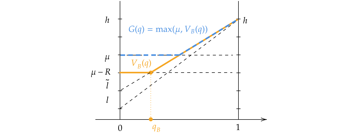
Figure 3: $V_{B}$ defined in (3.8) (in orange) v.s. $G$ defined in (2.24) (in dashed blue).

Proof.

The boundary conditions $V_{B}(0)=\mu-R$ and $V_{B}(1)=h$ follow directly. The form of equation (3.7) also follows, observing that

$$\lambda\widetilde{q}\left(V_{B}(1)-V_{B}(\widetilde{q})\right)+\lambda(1-\widetilde{q})\left(V_{B}(0)-V_{B}(\widetilde{q})\right)=\lambda(\widetilde{q}h+(1-\widetilde{q})(\mu-R)-V_{B}(\widetilde{q})).$$

Assertions (3.9) and (3.10) are obvious. ∎

The value function $V$ (cf. (3.3)) is then given by the optimal stopping problem

$$V(q)=\sup_{\tau\in\mathcal{T}_{Y}}\mathbb{E}\left[\left.-\int_{0}^{\tau}e^{-\rho t}C(q_{t})dt+e^{-\rho\tau}\widetilde{G}(q_{\tau})\,\right|q_{0}=q\right],$$ (3.11)

where

$$\widetilde{G}(q)=\max\left(\mu,\,V_{B}(q)\right),$$

with $\,V_{B}(q)$ as in (3.8). Note that because of the form of $\,V_{B},$ the obstacle term $\widetilde{G}(q)$ has a similar, piece-wise structure to the one in the irreversible case with $G(q)=\max(\mu,qh+(1-q)l),$ with the only difference being that the constant $l$ (representing the low value of the unknown product $B$) is now replaced by $\widetilde{l}$ in (3.6). As a consequence, the results in Proposition 11  are directly applicable. We stress, however, that while problems (3.11) and (2.34) appear technically similar, they are generated by very different decision making models.

3.1.1 Constant information cost

To derive various properties of the value function $V(q),\ q\in[0,1]$ and compare them to their analogues in the irreversible case, we work in the case $C(q)=C_{I}>0$. Then, (3.3) becomes

$${\min}\left(\rho V(q)-\frac{1}{2}\left(\frac{h-l}{\sigma}\right)^{2}q^{2}(1-q)^{2}V^{\prime\prime}\left(q\right)+C_{I},V(q)-\max\Big{(}\mu,\,V_{B}(q)\Big{)}\right)=0,$$ (3.12)

with $V_{B}$ as in (3.8).

Theorem 13.

There exists a unique pair $(\underline{q},\overline{q}),$ with $0<\underline{q}<\overline{q}<1,$ such that the value function $V(q)\in\mathcal{C}^{1}([0,1])$ and satisfies

$$V(q)=\begin{cases}\mu,\quad&q\leq\underline{q},\\ d_{1}q^{\frac{1-k}{2}}(1-q)^{\frac{1+k}{2}}+d_{2}(1-q)^{\frac{1-k}{2}}q^{\frac{1+k}{2}}{-}\frac{C_{I}}{\rho},\quad&\underline{q}\leq q\leq\overline{q},\\ qh+(1-q)\widetilde{l},\quad&\overline{q}\leq q,\end{cases}$$

with $\widetilde{l}$ defined in (3.6), $k$ as in (2.36),

$$d_{1}=\frac{\frac{1+k}{2}-\underline{q}}{k(1-\underline{q})^{\frac{1+k}{2}}\underline{q}^{\frac{1-k}{2}}}\left({\mu}+\frac{C_{I}}{\rho}\right),\text{ and }\ \ d_{2}=-\frac{\frac{1-k}{2}-\underline{q}}{k(1-\underline{q})^{\frac{1-k}{2}}\underline{q}^{\frac{1+k}{2}}}\left({\mu}+\frac{C_{I}}{\rho}\right).$$

Proof.

The ODE

$$\rho V-\frac{(h-l)^{2}}{2\sigma^{2}}q^{2}(1-q)^{2}V^{\prime\prime}+C_{I}=0$$ (3.13)

has a general solution given by

$$V(q)=d_{1}v_{1}(q)+d_{2}v_{2}(q)-\frac{C_{I}}{\rho},$$ (3.14)

where $d_{1},d_{2}$ are parameters to be determined, and

$$v_{1}(q)=q^{\frac{1-k}{2}}(1-q)^{\frac{1+k}{2}},\quad v_{2}(q)=q^{\frac{1+k}{2}}(1-q)^{\frac{1-k}{2}},$$

with $k$ as in (2.36).

Working as in Theorem 5 we deduce that there exist $\underline{q},\overline{q}$ with $0<\underline{q}<\overline{q}<1$, such that $V(q)=\mu,$ for $q\in[0,\underline{q}]$; $V(q)=qh+(1-q)\,\widetilde{l},$ for $q\in[\overline{q},1]$; and $V(q)$ satisfies the ODE (3.13) for $q\in[\underline{q},\overline{q}]$. Therefore, by the smooth-fit principle, $d_{1},d_{2},\underline{q},\overline{q}$ need to satisfy

$$\begin{cases}d_{1}v_{1}(\underline{q})+d_{2}v_{2}(\underline{q})-\frac{C_{I}}{\rho}&={\mu},\\ d_{1}v_{1}^{\prime}(\underline{q})+d_{2}v_{2}^{\prime}(\underline{q})&=0,\\ d_{1}v_{1}(\overline{q})+d_{2}v_{2}(\overline{q})-\frac{C_{I}}{\rho}&=\overline{q}h+(1-\overline{q})\,\widetilde{l},\\ d_{1}v_{1}^{\prime}(\overline{q})+d_{2}v_{2}^{\prime}(\overline{q})&=h-\,\widetilde{l}.\end{cases}$$

Technically, two of the four equations above are sufficient to write $d_{1},d_{2}$ in terms of $\overline{q},\underline{q}$. For simplicity, we write both $d_{1}$ and $d_{2}$ in terms of $\underline{q}$ which utilizes the first two equations. To simplify the notation, denote $m:=\frac{1-k}{2}$. Then, the general solution (3.14) can be written as

$$V(q)=d_{1}q^{m}(1-q)^{-m+1}+d_{2}(1-q)^{m}q^{-m+1}-\frac{C_{I}}{\rho}.$$

In turn,

$$V^{\prime}(q) = d_{1}mq^{m-1}(1-q)^{-m+1}+d_{1}(m-1)q^{m}(1-q)^{-m}$$

$$+d_{2}(-m)(1-q)^{m-1}q^{-m+1}+d_{2}(-m+1)(1-q)^{m}q^{-m}$$

$$= d_{1}q^{m-1}(1-q)^{-m}\left(m(1-q)+(m-1)q\right)+d_{2}(1-q)^{m-1}q^{-m}\left(-mq+(-m+1)(1-q)\right)$$

$$= d_{1}q^{m-1}(1-q)^{-m}(m-q)+d_{2}(1-q)^{m-1}q^{-m}\left(-m+1-q\right).$$

At point $\underline{q}$, we must have

$$d_{1}\underline{q}^{m}(1-\underline{q})^{-m+1}+d_{2}(1-\underline{q})^{m}\underline{q}^{-m+1}={\mu}+\frac{C_{I}}{\rho},$$ (3.15)

$$d_{1}(m-\underline{q})\underline{q}^{m-1}(1-\underline{q})^{-m}+d_{2}\left(-m+1-\underline{q}\right)(1-\underline{q})^{m-1}\underline{q}^{-m}=0.$$ (3.16)

From (3.16), we then obtain

$$d_{1}=-d_{2}\frac{-m+1-\underline{q}}{m-\underline{q}}\frac{(1-\underline{q})^{m-1}\underline{q}^{-m}}{\underline{q}^{m-1}(1-\underline{q})^{-m}}=-d_{2}\frac{-m+1-\underline{q}}{m-\underline{q}}\frac{(1-\underline{q})^{2m-1}}{\underline{q}^{2m-1}}.$$ (3.17)

Plugging the above equation into (3.15) gives

$$-d_{2}\frac{-m+1-\underline{q}}{m-\underline{q}}\frac{(1-\underline{q})^{2m-1}}{\underline{q}^{2m-1}}\underline{q}^{m}(1-\underline{q})^{-m+1}+d_{2}(1-\underline{q})^{m}\underline{q}^{-m+1}={\mu}+\frac{C_{I}}{\rho}.$$

By direct computation, we deduce

$$-d_{2}\frac{-m+1-\underline{q}}{m-\underline{q}}(1-\underline{q})^{m}q^{-m+1}+d_{2}(1-\underline{q})^{m}(\underline{q})^{-m+1}={\mu}+\frac{C_{I}}{\rho}.$$

Hence $d_{2}\left(1-\frac{-m+1-\underline{q}}{m-\underline{q}}\right)(1-\underline{q})^{m}\underline{q}^{-m+1}={\mu}+\frac{C_{I}}{\rho}$ and, in turn,

$$d_{2}=\left({\mu}+\frac{C_{I}}{\rho}\right)\frac{m-\underline{q}}{2m-1}(1-\underline{q})^{-m}\underline{q}^{m-1}.$$ (3.18)

Plugging (3.18) into (3.17), gives

$$d_{1}=-\left({\mu}+\frac{C_{I}}{\rho}\right)\frac{-m+1-\underline{q}}{2m-1}(1-\underline{q})^{m-1}\underline{q}^{-m}.$$

∎

Next, we investigate how the exchange penalty $R$ affects the actions of the DM in the first exploration period $[0,\tau^{\ast}]$.

Proposition 14.

Fix the values of $l$, $\mu$, $h$, $\rho$, $C_{I}$, $\sigma$, and $\lambda$. If the exchange fee $R$ increases, then both $\underline{q}$ and $\overline{q}$ increase.

Proof.

Let $R_{2}<R_{1}$ and denote $\widetilde{l}_{1},\widetilde{l}_{2}$ as in (3.6) with $R_{1}$,$R_{2}$ respectively. Then we have $\widetilde{l}_{1}<\widetilde{l}_{2}$. Let

$$\widetilde{G}_{1}(q)=\max\left(\mu,qh+(1-q)\widetilde{l}_{1}\right)\text{ \ \ and \ \ }\widetilde{G}_{2}(q)=\max\left(\mu,qh+(1-q)\widetilde{l}_{2}\right),$$

and note that, for $q\in\left[0,1\right],$

$$\frac{h-\widetilde{l}_{2}}{h-\widetilde{l}_{1}}\widetilde{G}_{1}(q)+\frac{\widetilde{l}_{2}-\widetilde{l}_{1}}{h-\widetilde{l}_{1}}h\,\geq\,\widetilde{G}_{2}(q)\,\geq\,\widetilde{G}_{1}(q).$$

Let $V_{1}$ and $V_{2}$ be the respective viscosity solutions to

$$\min\left(\rho V_{1}(q)-\frac{1}{2}\left(\frac{h-l}{\sigma}\right)^{2}q^{2}(1-q)^{2}V_{1}^{\prime\prime}(q)+C_{I},V_{1}(q)-\widetilde{G}_{1}(q)\right) =0,$$ (3.19)

$$\min\left(\rho V_{2}(q)-\frac{1}{2}\left(\frac{h-l}{\sigma}\right)^{2}q^{2}(1-q)^{2}V_{2}^{\prime\prime}(q)+C_{I},V_{2}(q)-\widetilde{G}_{2}(q)\right) =0.$$ (3.20)

Using that $\widetilde{G}_{1}(q)\leq\widetilde{G}_{2}(q)$ and working as in the proof of Proposition 11 herein, we deduce that $V_{1}$ is a viscosity subsolution to (3.20) and, by comparison, we conclude that $V_{1}\left(q\right)\leq V_{2}\left(q\right)$.

Next, we show that the function $\frac{h-\widetilde{l}_{2}}{h-\widetilde{l}_{1}}V_{1}+\frac{\widetilde{l}_{2}-\widetilde{l}_{1}}{h-\widetilde{l}_{1}}h$ is a viscosity supersolution to (3.20). For this, we take $q_{0}\in(0,1)$ and a test function $\psi\in\mathcal{C}^{2}((0,1))$, such that

$$\left(\frac{h-\widetilde{l}_{2}}{h-\widetilde{l}_{1}}V_{1}+\frac{\widetilde{l}_{2}-\widetilde{l}_{1}}{h-\widetilde{l}_{1}}h-\psi\right)(q_{0})=\min_{q\in(0,1)}\left(\frac{h-\widetilde{l}_{2}}{h-\widetilde{l}_{1}}V_{1}\left(q\right)+\frac{\widetilde{l}_{2}-\widetilde{l}_{1}}{h-\widetilde{l}_{1}}h\left(q\right)-\psi\left(q\right)\right)=0.$$

Then, the test function $\varphi:=\frac{h-\widetilde{l}_{1}}{h-\widetilde{l}_{2}}\left(\psi-\frac{\widetilde{l}_{2}-\widetilde{l}_{1}}{h-\widetilde{l}_{1}}h\right)$ satisfies $\varphi\in\mathcal{C}^{2}((0,1))$ and

$$(V_{1}-\varphi)(q_{0})=\min_{q\in(0,1)}(V_{1}\left(q\right)-\varphi\left(q\right))=0.$$

Since $V_{1}$ is the viscosity solution to (3.19), it is a viscosity supersolution to (3.19) and, thus,

$$\min\left(\rho\varphi(q_{0})-\frac{1}{2}\left(\frac{h-l}{\sigma}\right)^{2}q_{0}^{2}(1-q_{0})^{2}\varphi^{\prime\prime}(q_{0})+C_{I},\varphi(q_{0})-\widetilde{G}_{1}(q_{0})\right)\geq 0.$$

On the other hand, $\varphi\leq\frac{h-\widetilde{l}_{1}}{h-\widetilde{l}_{2}}\psi$, $\varphi^{\prime\prime}=\frac{h-\widetilde{l}_{1}}{h-\widetilde{l}_{2}}\psi^{\prime\prime}$, $C_{I}\leq\frac{h-\widetilde{l}_{1}}{h-\widetilde{l}_{2}}C_{I}$, and $\varphi-\widetilde{G}_{1}=\frac{h-\widetilde{l}_{1}}{h-\widetilde{l}_{2}}\psi-\frac{\widetilde{l}_{2}-\widetilde{l}_{1}}{h-\widetilde{l}_{2}}h-\widetilde{G}_{1}\leq\frac{h-\widetilde{l}_{1}}{h-\widetilde{l}_{2}}(\psi-\widetilde{G}_{2})$, and, thus,

$$\min\left(\rho\psi(q_{0})-\frac{1}{2}\left(\frac{h-l}{\sigma}\right)^{2}q_{0}^{2}(1-q_{0})^{2}\psi^{\prime\prime}(q_{0})+C_{I},\psi(q_{0})-\widetilde{G}_{2}(q_{0})\right)\geq 0.$$

Therefore, $\frac{h-\widetilde{l}_{2}}{h-\widetilde{l}_{1}}V_{1}+\frac{\widetilde{l}_{2}-\widetilde{l}_{1}}{h-\widetilde{l}_{1}}h$ is a viscosity supersolution to (3.20) and, in turn, the comparison principle yields that it dominates $V_{2}.$ In summary, we have so far shown that

$$\frac{h-\widetilde{l}_{2}}{h-\widetilde{l}_{1}}V_{1}(q)+\frac{\widetilde{l}_{2}-\widetilde{l}_{1}}{h-\widetilde{l}_{1}}h\geq V_{2}(q)\geq V_{1}(q),\text{ \ \ }q\in[0,1].$$

By Theorem 5, there exist two pairs of cutoff points $\left(\underline{q}_{1},\overline{q}_{1}\right)$   and $\ \left(\underline{q}_{2},\overline{q}_{2}\right)$ such that

$$\begin{cases}V_{1}(q)=\mu,&q\in[0,\underline{q}_{1}],\\ V_{1}(q)>\widetilde{G}_{1}(q),&q\in(\underline{q}_{1},\overline{q}_{1}),\\ V_{1}(q)=hq+\widetilde{l}_{1}(1-q),&q\in[\overline{q}_{1},1],\end{cases}\qquad\begin{cases}V_{2}(q)=\mu,&q\in[0,\underline{q}_{2}],\\ V_{2}(q)>\widetilde{G}_{2}(q),&q\in(\underline{q}_{2},\overline{q}_{2}),\\ V_{2}(q)=hq+\widetilde{l}_{2}(1-q),&q\in[\overline{q}_{2},1].\end{cases}$$

To compare $\underline{q}_{1}$ and $\underline{q}_{2}$, note that $V_{2}(q)\geq V_{1}(q)\geq\mu.$ For any $q\in[0,1]$ such that $V_{2}(q)=\mu$, we also have $V_{1}(q)=\mu$ and, hence,

$$[0,\underline{q}_{2}]=\{q\in[0,1]:V_{2}(q)=\mu\}\subseteq\{q\in[0,1]:V_{1}(q)=\mu\}=[0,\underline{q}_{1}],$$

which implies that $\underline{q}_{2}\leq\underline{q}_{1}$. Analogously, to compare $\overline{q}_{1},\overline{q}_{2}$, we observe that

$$\frac{h-\widetilde{l}_{2}}{h-\widetilde{l}_{1}}V_{1}+\frac{\widetilde{l}_{2}-\widetilde{l}_{1}}{h-\widetilde{l}_{1}}h\geq\frac{h-\widetilde{l}_{2}}{h-\widetilde{l}_{1}}(hq+\widetilde{l}_{1}(1-q))+\frac{\widetilde{l}_{2}-\widetilde{l}_{1}}{h-\widetilde{l}_{1}}h=hq+\widetilde{l}_{2}(1-q).$$

For any $q\in[0,1]$ such that $V_{1}(q)=hq+\widetilde{l}_{1}(1-q)$, we also have $V_{2}(q)=hq+\widetilde{l}_{2}(1-q)$ and, therefore,

$$[\overline{q}_{1},1]=\{q\in[0,1]:V_{1}(q)=hq+\widetilde{l}_{1}(1-q)\}$$

$$\subseteq\{q\in[0,1]:V_{2}(q)=hq+\widetilde{l}_{2}(1-q)\}=[\overline{q}_{2},1],$$

which yields $\overline{q}_{2}\leq\overline{q}_{1}$.

In conclusion, for $\widetilde{l}_{2}>\widetilde{l}_{1}$, i.e. $R_{2}<R_{1}$, we have $\underline{q}_{2}\leq\underline{q}_{1}$ and $\overline{q}_{2}\leq\overline{q}_{1}$. ∎

Proposition 14 implies that, when the return fee $R$ increases, the DM becomes more reluctant to leave the safe choice region (since $\underline{q}$ increases) and take the risk to choose product $B$ (since $\overline{q}$ increases).

Comparison with the single (irreversible) decisions.

As mentioned earlier, $\widetilde{G}(q)$ has the same structure as the $G(q)$ function, by replacing $l$ by $\widetilde{l}$. Hence the solution of the extended model with a Poisson-type refined signal may be viewed as a single (irreversible) problem with a modified low value for the unknown product. Conceptually, however, we are dealing with distinct model settings.

The quantity $\widetilde{l}$ decreases when the return fee $R$ increases, with the limiting value $\widetilde{l}=l$ achieved when $R=\mu-l$. By rewriting $\widetilde{l}=-\frac{\rho}{\rho+\lambda}(\mu-R-l)+(\mu-R)$, we also see that $\widetilde{l}$ increases when $\lambda$ increases.

Proposition 11 suggests that, asymptotically, the bandwidth of the exploration region $[\underline{q},\overline{q}]$ converges to zero as $\lambda\uparrow\infty$ and $R\downarrow 0$. This implies that when the Poisson signal arrives fast enough and when the cost of switching is low, the DM will spend less time acquiring costly information in the first exploratory period, and will make her initial choice comparatively sooner than in the single (irreversible) case.

3.2 Case 2: Gaussian signal of higher accuracy

The new observation process $\widetilde{Y}$ is modeled as

$$d\widetilde{Y}_{t}=\Theta\,dt+\widetilde{\sigma}d\widetilde{W}_{t},$$ (3.21)

with $0<\widetilde{\sigma}\leq\sigma,$ $\sigma$ being the volatility coefficient of the signal $Y$ used in the first exploratory period, and $\widetilde{W}_{t}$ is a standard Brownian motion independent of $W_{t}$. In analogy, the related belief process $\widetilde{q}$ solves (3.22),

$$d\widetilde{q}_{t}=\frac{h-l}{\widetilde{\sigma}}\widetilde{q}_{t}\left(1-\widetilde{q}_{t}\right)d\widetilde{Z}_{t},\text{ \ }\widetilde{q}_{0}=\widetilde{q}\in\left[0,1\right],$$ (3.22)

with $\widetilde{Z}$ being a standard Brownian motion in $\left(\Omega,\mathcal{F},\left\{\mathcal{F}_{t}^{\widetilde{Y}}\right\},\mathbb{P}\right)$. The corresponding variational inequality for the nested continuation value function of product $B$ is

$${\min}\left(\rho{V}_{B}(\widetilde{q})-\frac{1}{2}\left(\frac{h-l}{\widetilde{\sigma}}\right)^{2}\widetilde{q}^{2}(1-\widetilde{q})^{2}V_{B}^{\prime\prime}(\widetilde{q})-\rho\left(\widetilde{q}h+(1-\widetilde{q})l\right),{V}_{B}(\widetilde{q})-\left(\mu-R\right)\right)=0,$$

with $V_{B}(0)=\mu-R$ and $V_{B}(1)=h.$

Proposition 15.

The nested continuation value function for product $B{\ }$is given by

$${V}_{B}(\widetilde{q})=\begin{cases}\mu-R,\quad&\widetilde{q}\leq q_{B},\\ \widetilde{q}h+(1-\widetilde{q})l+{d}_{B}\widetilde{q}^{\frac{1-\widetilde{k}}{2}}(1-\widetilde{q})^{\frac{1+\widetilde{k}}{2}},\quad&\widetilde{q}>q_{B},\end{cases}$$ (3.23)

where

$$q_{B}=\frac{\left(l-\mu+R\right)\left(\frac{1-\widetilde{k}}{2}\right)}{(h-l)\left(\frac{1+\widetilde{k}}{2}\right)+l-\mu+R},$$

with

$${d}_{B}=\frac{\mu-R-q_{B}h-(1-q_{B})l}{q_{B}{}^{\frac{1-\widetilde{k}}{2}}(1-\widetilde{q}_{B})^{\frac{1+\widetilde{k}}{2}}}\text{ \ \ and \ \ }\widetilde{k}=\sqrt{1+8\rho\left(\frac{\widetilde{\sigma}}{h-l}\right)^{2}}.$$ (3.24)

Proof.

We first note that the solution of the ODE (with a slight abuse of notation)

$$\rho V_{B}(\widetilde{q})-\frac{1}{2}\left(\frac{h-l}{\widetilde{\sigma}}\right)^{2}\widetilde{q}^{2}(1-\widetilde{q})^{2}V_{B}^{\prime\prime}(\widetilde{q})-\rho\Big{(}\widetilde{q}h+(1-\widetilde{q})l\Big{)}=0$$ (3.25)

can be written as

$$V_{B}(\widetilde{q})=\widetilde{q}h+(1-\widetilde{q})l+c_{1}v_{1}(\widetilde{q})+c_{2}v_{2}(\widetilde{q}),$$

where

$$v_{1}(\widetilde{q})=\widetilde{q}^{\frac{1-\widetilde{k}}{2}}(1-\widetilde{q})^{\frac{1+\widetilde{k}}{2}},\quad v_{2}(\widetilde{q})=\widetilde{q}^{\frac{1+\widetilde{k}}{2}}(1-\widetilde{q})^{\frac{1-\widetilde{k}}{2}},$$

$c_{1}$ and $c_{2}$ two free parameters to be determined, and $\widetilde{k}$ as in (3.24).

Working as in the proof of Proposition 12, we seek ${V}_{B}\in\mathcal{C}^{1}([0,1])$ and $q_{B}\in(0,1)$ such that ${V}_{B}(\widetilde{q})=\mu-R,$ $q\leq\widetilde{q}_{B}$, and ${V}_{B}(\widetilde{q})$ satisfies ODE (3.25) for $\widetilde{q}>q_{B}$.

Since $V_{B}$ is bounded near $\widetilde{q}=1$ we conclude that $c_{2}=0$, otherwise we would have $\lim_{\widetilde{q}\rightarrow 1}|V_{B}(\widetilde{q})|=+\infty$ since $\lim_{\widetilde{q}\rightarrow 1}v_{2}(\widetilde{q})=\infty$. We introduce the notation $d_{B}=c_{1}$.

Applying the smooth fit principle yields

$$q_{B}h+(1-q_{B})l+d_{B}q_{B}{}^{\frac{1-\widetilde{k}}{2}}(1-{q}_{B})^{\frac{1+\widetilde{k}}{2}}=\mu-R,$$

$$h-l+d_{B}q_{B}{}^{-\frac{1+\widetilde{k}}{2}}(1-q_{B})^{-\frac{1-\widetilde{k}}{2}}\left(\frac{1-\widetilde{k}}{2}-{q}_{B}\right)=0,$$

which, in turn, implies

$$q_{B} = \frac{\left(l-\mu+R\right)\left(\frac{1-\widetilde{k}}{2}\right)}{(h-l)\left(\frac{1+\widetilde{k}}{2}\right)+l-\mu+R},$$

$${d}_{B} = \frac{\mu-R-q_{B}h-(1-q_{B})l}{q_{B}{}^{\frac{1-\widetilde{k}}{2}}(1-{q}_{B})^{\frac{1+\widetilde{k}}{2}}}.$$

∎

We now provide some properties of the terminal condition.

Lemma 16.

If $R>0$, there exists a unique $q^{\prime}\in(0,1)$ such that $V_{B}(q^{\prime})=\mu$.

Proof.

Since $V_{B}(q_{B})=\mu-R<\mu$ and $V_{B}(1)=h>\mu$, by the continuity of $V_{B}$ there exists, at least, one $\widetilde{q}\in(q_{B},1)$ such that $V_{B}(\widetilde{q})=\mu$.

Moreover, using the form of $V_{B}$, we can show that for $\widetilde{q}\in(q_{B},1)$, we have

$$V_{B}^{\prime\prime}(\widetilde{q})=\frac{d_{B}(\widetilde{k}^{2}-1)}{4\widetilde{q}^{\frac{3+\widetilde{k}}{2}}(1-\widetilde{q})^{\frac{3-\widetilde{k}}{2}}}>0.$$

Therefore, $V_{B}(\widetilde{q})$ is convex for $\widetilde{q}\in(q_{B},1)$. Next, suppose there exist at least two points $q_{1}$ and $q_{2}$ such that $V_{B}(q_{1})=V_{B}(q_{2})=\mu$, with $\widetilde{q}_{B}<q_{1}<q_{2}<1$. Then, by the convexity of $V_{B}$, we must have

$$V_{B}(q_{1})\leq\frac{q_{2}-q_{1}}{q_{2}-q_{B}}V_{B}(\widetilde{q}_{B})+\frac{q_{1}-q_{B}}{q_{2}-q_{B}}V_{B}(q_{2})<\mu,$$

which, however, contradicts that $V_{B}(q_{1})=\mu$. Therefore, there must be a unique point $q^{\prime}$ such that $V(q^{\prime})=\mu$. See Figure 4 for a demonstration.

∎

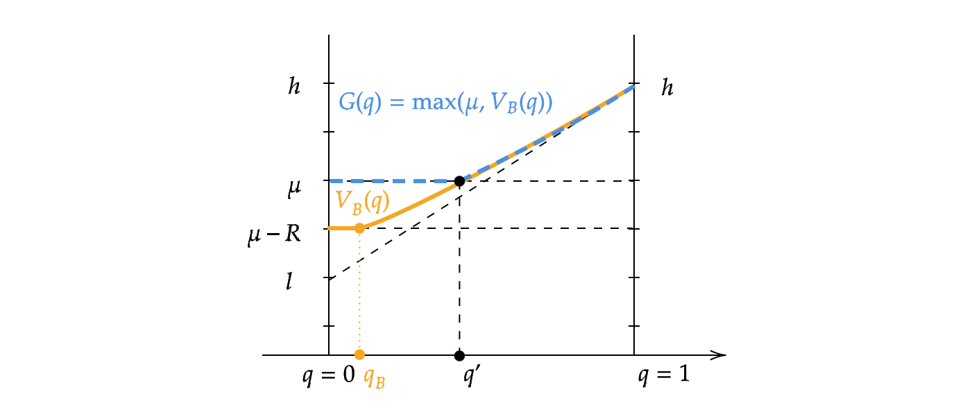
Figure 4: $V_{B}$ defined in (3.23) (in orange) v.s. $G$ defined in (2.24) (in dashed blue).

3.2.1 Constant information cost

We assume that $C(q)=C_{I}>0,$ $q\in\left[0,1\right]$. Then the value function $V$ satisfies

$${\min}\left(\rho V(q)-\frac{1}{2}\left(\frac{h-l}{\sigma}\right)^{2}q^{2}(1-q)^{2}V^{\prime\prime}\left(q\right)+C_{I},V(q)-\widetilde{G}(q)\right)=0.$$

where

$$\widetilde{G}(q)=\max\Big{(}\mu,V_{B}(q)\Big{)}$$

with $V_{B}$ given in (3.23). Working as in the proof of Theorem 13 we deduce the following result. The arguments are similar, albeit more tedious but are omitted for brevity.

Theorem 17.

There exists a unique pair $(\underline{q},\overline{q})$, with $0<\underline{q}<\overline{q}<1$, such that the value function $V(q)\in\mathcal{C}^{1}\left(\left[0,1\right]\right)$ and satisfies

$$V(q)=\begin{cases}{\mu},\quad&q\leq\underline{q},\\ d_{1}q^{\frac{1-k}{2}}(1-q)^{\frac{1+k}{2}}+d_{2}(1-q)^{\frac{1-k}{2}}q^{\frac{1+k}{2}}-\frac{C_{I}}{\rho},\quad&\underline{q}\leq q\leq\overline{q},\\ qh+(1-q)l+d_{B}q^{\frac{1-\widetilde{k}}{2}}(1-q)^{\frac{1+\widetilde{k}}{2}},\quad&\overline{q}\leq q,\end{cases}$$

where

$$d_{1}=\frac{\frac{1+k}{2}-\underline{q}}{k(1-\underline{q})^{\frac{1+k}{2}}\underline{q}^{\frac{1-k}{2}}}\left({\mu}+\frac{C_{I}}{\rho}\right)\text{, \ }d_{2}=-\frac{\frac{1-k}{2}-\underline{q}}{k(1-\underline{q})^{\frac{1-k}{2}}\underline{q}^{\frac{1+k}{2}}}\left({\mu}+\frac{C_{I}}{\rho}\right),$$

and

$$d_{B}=\frac{\mu-l-R}{\frac{1+\widetilde{k}}{2}}\left(\frac{\left(\frac{1+\widetilde{k}}{2}\right)(h-\mu+R)}{-\left(\frac{1-\widetilde{k}}{2}\right)(\mu-l-R)}\right)^{\frac{1-\widetilde{k}}{2}},$$

with $\widetilde{k}=\sqrt{1+8\rho\left(\frac{\widetilde{\sigma}}{h-l}\right)^{2}}$.

3.2.2 Comparison with the solution of the single (irreversible) decision problem

Analytically, as $\widetilde{\sigma}\downarrow 0$, we can show from Theorem 15, or using similar arguments as in Section 2.3.2, that $q_{B}\downarrow 0$ and $V_{B}(\widetilde{q})=\widetilde{q}h+(1-\widetilde{q})\left(\mu-R\right)$. Thus, we may view $\widetilde{G}(q)$ as the analogous $G(q)$ function in the irreversible decision making case but with the lower value of product $B$ replaced by $\mu-R$. This implies that, if the DM could observe immediately the true value of product $B$ should she choose it, she would immediately finalize her decision whether to keep it if $\Theta=h$, or switch to product $A$ at a cost of $R$, if $\Theta=l$.

Also note that when $\widetilde{\sigma}=0$, the same monotonicity result with respect to changes in $R$ in Proposition 14 holds, i.e., as $R$ increases, both $\underline{q}$ and $\overline{q}$ increase. This indicates that when the cost of revising the initial decision is higher, the DM is more likely to choose the well-known product $A$.

Finally, we further conduct a series of numerical experiments when $0<\widetilde{\sigma}<\sigma$, as illustrated in Figure 5, to further investigate the impact of the exchange cost $R$ on the behavior of DM.

Here we re-denote the cutoffs of the irreversible counterpart as $\underline{q}^{\ast}$ and $\overline{q}^{\ast}$. As $R$ increases from zero to $\mu-l$, we observe that:

• Both points, $\underline{q}$ and $\overline{q},$ increase monotonically and converge towards $\underline{q}^{\ast}$ and $\overline{q}^{\ast},$ respectively. This indicates that when the return becomes more costly, the behavior of the DM tends to align more closely with the one exhibited in single (irreversible) decision problem.

• The width of the exploration region $\overline{q}-\underline{q}$ also expands from zero to $\overline{q}^{\ast}-\underline{q}^{\ast}$ of the single (irreversible) decision problem. This shows that when the exchange cost is zero, the DM tends to make her initial choice without any exploration. This situation also presents a significant advantage for selecting product $B$ initially (since both $\underline{q}$ and $\overline{q}$ have a small value), as the DM can always switch to product $A$ at no additional cost later on. However, as the cost to return the unknown product increases, the DM engages in more exploration before reaching her initial decision in the first exploratory period.

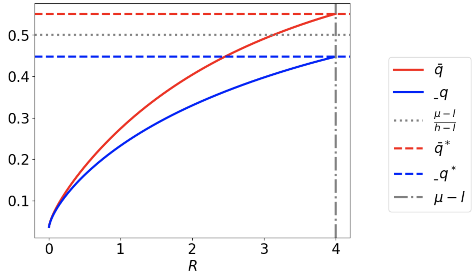
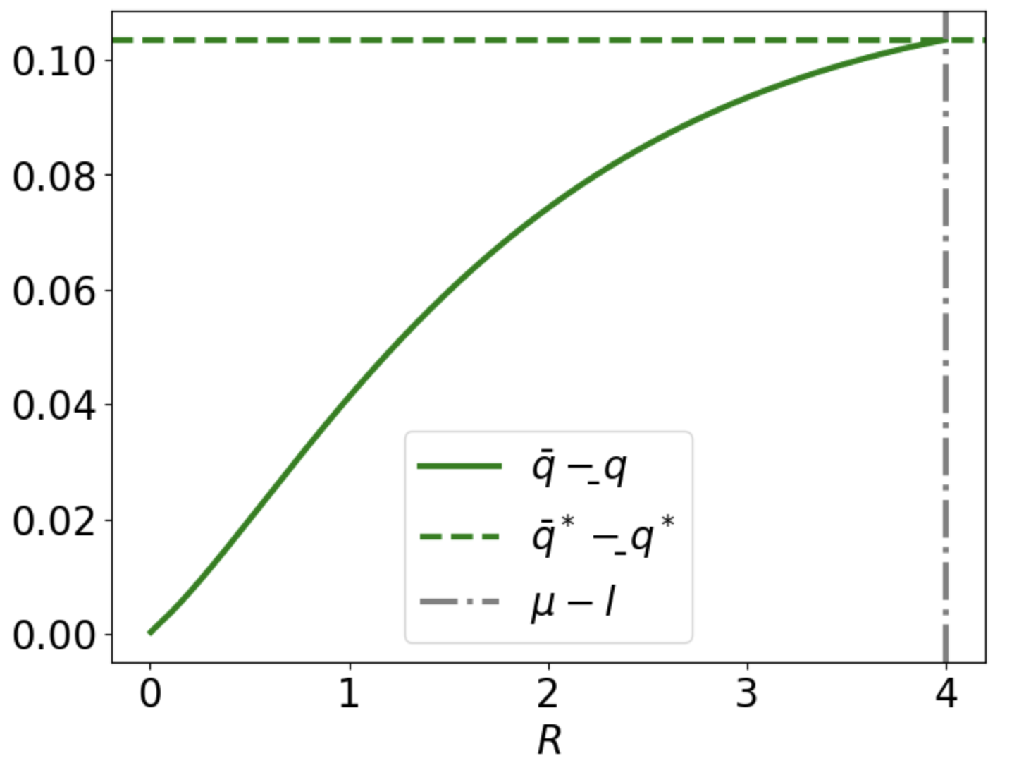
Figure 5: Behavior of $\underline{q}$, $\overline{q}$, and $\overline{q}-\underline{q}$. In this experiment, we take $\rho=1$, $l=1$, $h=9$, $\mu=5$, $c=1$, $\sigma=5$, $\widetilde{\sigma}=1$.

4 Conclusions and future research directions

We introduced and analyzed a new decision-making model with sequential decisions, costly information acquisition and distinct informational sources across time. We focused on an E-commerce model in which a DM is presented with the opportunity to choose between a well-known product and a new one about which she learns through a continuous-time signal. Acquiring information about the new product is costly and accumulates through time. The DM chooses a product but, contrary to the existing models, decision-making continues as she has the optionality to return it and exchange it with the other one and, in addition, she has access to a finer, more accurate source of information if she first chooses product $B$. On the other hand, returning the product is costly. We formulated the underlying optimal stopping problem which is a compilation of an “outer” and a “nested” optimal stopping problem with general payoffs and informational costs. We developed a viscosity solution toolkit and analyzed various cases, performed sensitivity analysis, and studied the limiting behavior of the solution in terms of the various model inputs.

There are various directions the current work may be extended. Firstly, it is important to allow for multiple signals in the different decision regimes, so that the DM also controls the type of information source. This is expected to give rise to nested optimal stopping problems with variance control (for the case of Gaussian signals). Secondly, one may extend the current setting to multiple DMs who complete product availability but share common informational sources. This is expected to give rise to a mean field game of control. Thirdly, the proposed model provides a flexible framework to study variable return fees and set up a separate optimization problem for their specification. Some of these questions are being currently investigated by the authors.

Appendix A Additional Proofs

Proof of Proposition 8.

We establish monotonicity in $\sigma$. For $\sigma_{2}>\sigma_{1}$, let $V_{1}$, $V_{2}$ be the viscosity solutions to

$$\min\left(\rho V_{1}(q)-\frac{1}{2}\left(\frac{h-l}{\sigma_{1}}\right)^{2}q^{2}(1-q)^{2}V_{1}^{\prime\prime}\left(q\right)+C(q),V_{1}(q)-G(q)\right) =0,$$ (A.1)

$$\min\left(\rho V_{2}(q)-\frac{1}{2}\left(\frac{h-l}{\sigma_{2}}\right)^{2}q^{2}(1-q)^{2}V_{2}^{\prime\prime}\left(q\right)+C(q),V_{2}(q)-G(q)\right) =0,$$ (A.2)

with $V_{1}\left(0\right)=V_{2}\left(0\right)=G(0)$ and $V_{1}\left(1\right)=V_{2}\left(1\right)=G(1)$. We show that $V_{2}$ is a viscosity subsolution to (A.1). Let $q_{0}\in(0,1)$ and consider a test function $\varphi\in\mathcal{C}^{2}((0,1))$ such that

$$(V_{2}-\varphi)(q_{0})=\max_{q\in\left(0,1\right)}(V_{2}-\varphi)\left(q\right)=0.$$

Since $V_{2}$ is a viscosity subsolution to (A.2), $\varphi$ must satisfy

$$\min\left(\rho\varphi(q_{0})-\frac{1}{2}\left(\frac{h-l}{\sigma_{2}}\right)^{2}q_{0}^{2}(1-q_{0})^{2}\varphi^{\prime\prime}(q_{0})+C(q_{0}),\varphi(q_{0})-G(q_{0})\right)\leq 0.$$

Therefore, either $\varphi(q_{0})-G(q_{0})\leq 0$ or

$$\varphi(q_{0})-G(q_{0})>0\text{ \ and \ }\rho\varphi(q_{0})-\frac{1}{2}\left(\frac{h-l}{\sigma_{2}}\right)^{2}q_{0}^{2}(1-q_{0})^{2}\varphi^{\prime\prime}\left(q_{0}\right)+C(q_{0})\leq 0.$$

The latter inequality implies that $\varphi^{\prime\prime}(q_{0})>0$ and, consequently,

$$\rho\varphi(q_{0})-\frac{1}{2}\left(\frac{h-l}{\sigma_{1}}\right)^{2}q_{0}^{2}(1-q_{0})^{2}\varphi^{\prime\prime}\left(q_{0}\right)+C(q_{0})<\rho\varphi(q_{0})-\frac{1}{2}\left(\frac{h-l}{\sigma_{2}}\right)^{2}q_{0}^{2}(1-q_{0})^{2}\varphi^{\prime\prime}\left(q_{0}\right)+C(q_{0})\leq 0.$$

Combining the above inequalities and using Lemma 7, we easily conclude. The rest of the proof follows easily. ∎

Proof of Proposition 9..

For $\mu_{2}>\mu_{1}$, let

$$G_{1}(q):=\max\Big{(}\mu_{1},qh+(1-q)l\Big{)}\text{ \ \ and \ \ }G_{2}(q)=:\max\Big{(}\mu_{2},qh+(1-q)l\Big{)}.$$

Then $G_{2}\left(q\right)\geq G_{1}\left(q\right)\geq G_{2}\left(q\right)-\mu_{2}+\mu_{1}$. Let $V_{1}$, $V_{2}$ be the viscosity solutions to

$$\min\left(\rho V_{1}(q)-\frac{1}{2}\left(\frac{h-l}{\sigma}\right)^{2}q^{2}(1-q)^{2}V_{1}^{\prime\prime}\left(q\right)+C\left(q\right),V_{1}(q)-G_{1}(q)\right) =0,$$ (A.3)

$$\min\left(\rho V_{2}(q)-\frac{1}{2}\left(\frac{h-l}{\sigma}\right)^{2}q^{2}(1-q)^{2}V_{2}^{\prime\prime}\left(q\right)+C\left(q\right),V_{2}(q)-G_{2}(q)\right) =0.$$ (A.4)

Let $q_{0}\in(0,1)$ and $\varphi\in\mathcal{C}^{2}((0,1))$ such that

$$(V_{1}-\varphi)(q_{0})=\max_{q\in\left(0,1\right)}(V_{1}-\varphi)\left(q\right)=0.$$

Since $V_{1}$ is the viscosity solution to (A.3) we have  

$$\min\left(\rho\varphi(q_{0})-\frac{1}{2}\left(\frac{h-l}{\sigma}\right)^{2}q_{0}^{2}(1-q_{0})^{2}\varphi^{\prime\prime}\left(q_{0}\right)+C(q_{0}),\varphi(q_{0})-G_{1}(q_{0})\right)\leq 0,$$

and, thus, using that $G_{1}(q)\leq G_{2}(q)$, we also have

$$\min\left(\rho\varphi(q_{0})-\frac{1}{2}\left(\frac{h-l}{\sigma}\right)^{2}q_{0}^{2}(1-q_{0})^{2}\varphi^{\prime\prime}\left(q_{0}\right)+C(q_{0}),\varphi(q_{0})-G_{2}(q_{0})\right)\leq 0,$$

which implies that $V_{1}$ is a viscosity subsolution to (A.3). By comparison, $V_{1}\leq V_{2}$.

Next, we show that the function $V_{2}-\mu_{2}+\mu_{1}$ is a viscosity subsolution to (A.3). For this, consider a test function $\psi\in\mathcal{C}^{2}((0,1))$, such that

$$(V_{2}-\mu_{2}+\mu_{1}-\psi)(q_{0}):=\max_{q\in\left(0,1\right)}(V_{2}-\mu_{2}+\mu_{1}-\psi)\left(q\right)=0.$$

Then, $\varphi:=\psi+\mu_{2}-\mu_{1}$ satisfies $\varphi\in\mathcal{C}^{2}((0,1))$ and

$$(V_{2}-\varphi)(q_{0})=\max_{q\in\left(0,1\right)}(V_{2}-\varphi)(q)=0.$$

Therefore,

$$\min\left(\rho\varphi(q_{0})-\frac{1}{2}\left(\frac{h-l}{\sigma}\right)^{2}q_{0}^{2}(1-q_{0})^{2}\varphi^{\prime\prime}\left(q_{0}\right)+C(q_{0}),\varphi(q_{0})-G_{2}(q_{0})\right)\leq 0.$$

Since $\varphi\geq\psi$, $\varphi^{\prime\prime}=\psi^{\prime\prime}$, and $\varphi-G_{2}=\psi+\mu_{2}-\mu_{1}-G_{2}\geq\psi-G_{1}$, we deduce that

$$\min\left(\rho\psi(q_{0})-\frac{1}{2}\left(\frac{h-l}{\sigma}\right)^{2}q_{0}^{2}(1-q_{0})^{2}\psi^{\prime\prime}\left(q_{0}\right)+C(q_{0}),\psi(q_{0})-G_{1}(q_{0})\right)\leq 0,$$

and, thus, $V_{2}-\mu_{2}+\mu_{1}$ is a viscosity subsolution to (A.3). By comparison, $V_{2}-\mu_{2}+\mu_{1}\leq V_{1}$.

So far we have shown that

$$V_{2}(q)-\mu_{2}+\mu_{1}\leq V_{1}(q)\leq V_{2}(q),\qquad q\in[0,1].$$

By Theorem 5 we know that there exist two pairs $\left(\underline{q}_{1},\overline{q}_{1}\right)$ and $\left(\underline{q}_{2},\overline{q}_{2}\right)$ such that

$$\begin{cases}V_{1}(q)=\mu_{1},&0\leq q\leq\underline{q}_{1}\\ V_{1}(q)>G_{1}(q),&\underline{q}_{1}<q<\overline{q}_{1}\\ V_{1}(q)=qh+(1-q)l,&\overline{q}_{1}\leq q\leq 1,\end{cases}\qquad\begin{cases}V_{2}(q)=\mu_{2},&0\leq q\leq\underline{q}_{2}\\ V_{2}(q)>G_{2}(q),&\underline{q}_{2}<q<\overline{q}_{2}\\ V_{2}(q)=qh+(1-q)l,&\overline{q}_{2}\leq q\leq 1.\end{cases}$$

To compare $\overline{q}_{1}$ and $\overline{q}_{2}$, notice that

$$V_{2}(q)\geq V_{1}(q)\geq qh+(1-q)l.$$

For any $q\in[0,1]$ such that $V_{2}(q)=qh+(1-q)l$, we also have $V_{1}(q)=qh+(1-q)l$. Therefore,

$$[\overline{q}_{2},1]=\Big{\{}q\in[0,1]:V_{2}(q)=qh+(1-q)l\Big{\}}\subseteq\Big{\{}q\in[0,1]:V_{1}(q)=qh+(1-q)l\Big{\}}=[\overline{q}_{1},1],$$

which yields $\overline{q}_{2}\geq\overline{q}_{1}$. To compare $\underline{q}_{1}$ and $\underline{q}_{2}$, notice that inequality $V_{2}(q)-\mu_{2}+\mu_{1}\leq V_{1}(q)$ yields

$$0\leq V_{2}(q)-\mu_{2}\leq V_{1}(q)-\mu_{1}.$$

For any $q\in[0,1]$ such that $V_{1}(q)=\mu_{1}$, we also have $V_{2}(q)=\mu_{2}$. Therefore,

$$[0,\underline{q}_{1}]=\{q\in[0,1]:V_{1}(q)=\mu_{1}\}\subseteq\{q\in[0,1]:V_{2}(q)=\mu_{2}\}=[0,\underline{q}_{2}],$$

which yields $\underline{q}_{2}\geq\underline{q}_{1}$. In conclusion, for $\mu_{2}>\mu_{1}$, we have $\underline{q}_{2}\geq\underline{q}_{1}$ and $\overline{q}_{2}\geq\overline{q}_{1}$. ∎

Proof of Proposition 10.

We only analyze the case $\sigma\uparrow+\infty$ as the other two follow similarly. To this end, we recall that $V$ is the viscosity solution to (2.14), rewritten for convenience,

$$\min\left(\rho V(q)-\frac{1}{2}\left(\frac{h-l}{\sigma}\right)^{2}q^{2}(1-q)^{2}V^{\prime\prime}\left(q\right)+C(q),V(q)-G(q)\right)=0,$$

with $G(q)=\max\left(\mu,qh+\left(1-q\right)l\right)$. We construct a suitable $\mathcal{C}^{1}((0,1))$ supersolution, introducing

$$U(q):=\begin{cases}\mu,&0\leq q\leq r\\ \mu+M(q-r)^{2},&r\leq q\leq p\\ qh+(1-q)l,&p\leq q\leq 1,\end{cases}$$

for some $r\in(0,\hat{p})$, $p\in(\hat{p},1)$ and $M>0$. To have $U\in\mathcal{C}^{1}(0,1)$, we need

$$U(p)=\mu+M(p-r)^{2}=ph+(1-p)l,$$ (A.5)

$$U^{\prime}(p)=2M(p-r)=h-l.$$ (A.6)

Note that, by construction, $U\left(q\right)=G\left(q\right)$ on $[0,r]\cup[p,1]$. Therefore, it suffices to verify that

$$\rho U(q)-\frac{1}{2}M\left(\frac{h-l}{\sigma}\right)^{2}q^{2}(1-q)^{2}+C(q)>0,\text{ \ }q\in[r,p],$$

which follows for large $\sigma.$ In turn, we use Lemma 7 to deduce that $r\leq\underline{q}\leq\overline{q}\leq p$.

We finish the proof by showing that the points $r$ and $p$ can be arbitrarily close to $\hat{p}$ (cf. (2.36)) if we choose $M$ sufficiently large. Indeed, applying (A.6) to (A.5) gives

$$\mu+\frac{(h-l)^{2}}{4M}=ph+(1-p)l=\mu+(h-l)(p-\hat{p}),$$

which yields $p=\hat{p}+\dfrac{h-l}{4M}.$ Using (A.6), we deduce that $r=\hat{p}-\dfrac{h-l}{4M}$. Hence $p\rightarrow\hat{p}$ and $r\rightarrow\hat{p},$ as $M\rightarrow\infty$. ∎

Proof of Proposition 11..

We first prove i). Note that $\hat{p}=\frac{\mu-l}{h-l}\downarrow 0$ when $l\uparrow\mu$. In this case, $\underline{q}\rightarrow 0$ as $\hat{p}\rightarrow 0$.

Next, we construct a suitable convex supersolution $U\in\mathcal{C}([0,1])$ to (2.14). For this, let

$$U(q):=\begin{cases}\mu,&q=0,\\ qh+(1-q)l+M(p-q)^{2},&0<q\leq p,\\ qh+(1-q)l,&p<q\leq 1,\end{cases}$$

for some $M>0$ and $p\in(\hat{p},1)$ to be determined in the sequel.

Firstly, note that continuity at $q=0$ requires $M$ and $p$ to satisfy $l+p^{2}M=\mu,$ and, thus,

$$p=\sqrt{\frac{\mu-l}{M}},$$

where $M$ will be chosen independently of $l$.

Next, we verify that $U$ is convex. Since $U^{\prime\prime}(q)=2M>0$, $q\in(0,p),$ and $U$ is affine on $[p,1]$, it suffices to compute the left derivative of $U$ at $p$. We have

$$U_{-}^{\prime}(p)=(h-l)+2M(p-p)=h-l.$$

Therefore, $U$ is convex in $[0,1]$ and piecewise smooth. Note also that $U^{\prime}(0)=h-l-2Mp>h-\mu-2Mp$, which is positive for $p$ sufficiently small as $l$ gets sufficiently close to $\mu$. Therefore, $U$ is strictly increasing in $[0,1]$.

We now verify that $U$ is a supersolution. Notice that $U\left(q\right)=G\left(q\right),$ for $q=0$ and $q\in[p,1]$. By monotonicity, $U(q)\geq U(0)=\mu$. From the definition, we also see $U(q)\geq qh+(1-q)l$, so $U\geq G$ in $[0,1]$. To show that $U$ is a supersolution, it suffices to establish that, for $q\in(0,p)$, it holds that

$$f(q):=\rho U(q)-\frac{1}{2}\left(\frac{h-l}{\sigma}\right)^{2}q^{2}(1-q)^{2}U^{\prime\prime}(q)+C(q)\geq 0.$$

Notice that

$$f(q)\geq\rho\mu+C_{1}-M\frac{h^{2}}{16\sigma^{2}}.$$

since $U(q)\geq\mu$ and $q^{2}(1-q)^{2}\leq\frac{1}{16},$ for $q\in[0,1]$. Recall that $C(q)\geq C_{1}$.

By taking $M=\frac{16(\rho\mu+C_{1})\sigma^{2}}{h^{2}}$, we have $f(q)\geq 0$. Therefore, choosing $p=\sqrt{\frac{\mu-l}{M}}$ and $M=\frac{16(\rho\mu+C_{1})\sigma^{2}}{h^{2}}$, we have that $U$ is a supersolution and $U(q)>G(q),$ $q\in(0,p)$. Then, by the comparison principle, we obtain that $V(q)\leq U(q),$ $q\in(0,p)$ and, hence, $p\geq\overline{q}$. As $l\rightarrow\mu$, we have $\underline{q}\rightarrow 0$ and $\overline{q}\rightarrow 0$ because ${\hat{p}}\rightarrow 0$ and $p\rightarrow 0$.

To show ii), we construct a convex subsolution $\overline{U}\in\mathcal{C}([0,1])$ with $\overline{U}=\max\left(\mu,U\right)$ for a suitable function $U.$ To this end, for some positive constants $m,M>0,r\in\left(0,\frac{1}{2}\right]$ and $p\in\left(\frac{1}{2},1\right)$ to be determined, we define

$$U(q):=\int_{q}^{1}\Phi(t)dt+qh+(1-q)l$$

(shown in Figure 6), where

$$U^{\prime\prime}(q)=\varphi(q)=\begin{cases}M,&0\leq q\leq r,\\ m,&r<q\leq p,\\ 0,&p<q\leq 1,\end{cases}\quad\Phi(q)=\int_{q}^{1}\varphi(t)dt=\begin{cases}m(p-r)+M(r-q),&0\leq q\leq r,\\ m(p-q),&r<q\leq p,\\ 0,&p<q\leq 1.\end{cases}$$

We choose $m,M,r$ independently of $h$. We claim that by a proper choice of $m,M,p,r$, $U$ will satisfy the following properties.

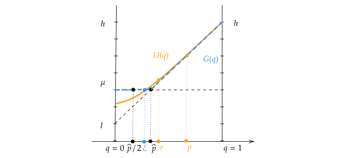
Figure 6: Illustration of $U(q)$ (orange solid line) and $G(q)=\max\big{(}\mu,qh+(1-q)l\big{)}$ (blue dotted line).

Firstly, $U$ is convex since $U^{\prime}(q)=-\Phi(q)+h-l$ is increasing in $q$. Moreover, $\Phi$ is Lipschitz, and $U$ is $\mathcal{C}([0,1])$ since $\varphi$ is bounded by $\max\left(m,M\right)$. We also have

$$U^{\prime}(0)=-\Phi(0)+h-l=-m(p-r)-Mr+h-l>-M+h-l,$$

where $M$ (as mentioned above) will be chosen independently of $h$. We have $U^{\prime}(0)>0,$ for $h$ is sufficiently large.

Next, we determine $\xi$ at which $U(\xi)=\mu$. By direct calculation,

$$U\left(\frac{\hat{p}}{2}\right) =\int_{\frac{\hat{p}}{2}}^{1}\Phi(t)dt+h\frac{\hat{p}}{2}+l\left(1-\frac{\hat{p}}{2}\right)$$ (A.7)

$$=\int_{\frac{\hat{p}}{2}}^{1}\Phi(t)dt+h\hat{p}+l\left(1-\hat{p}\right)-\frac{\hat{p}}{2}(h-l)$$ (A.8)

$$\leq\int_{0}^{1}\Phi(t)dt+\mu-\frac{1}{2}(\mu-l)$$ (A.9)

$$=mr(p-r)+\frac{M}{2}r^{2}+\frac{m}{2}(p-r)^{2}+\mu-\frac{1}{2}(\mu-l)$$ (A.10)

$$<\frac{1}{2}m+\frac{1}{2}Mr^{2}+\mu-\frac{1}{2}(\mu-l)<\mu,$$ (A.11)

if we choose $m=\frac{1}{2}(\mu-l)$, and $Mr^{2}=\frac{1}{2}(\mu-l)$. Since $U(\hat{p})>\hat{p}h+(1-\hat{p})l=\mu$, and $U$ is monotonically increasing, there exists a unique $\xi\in(\frac{\hat{p}}{2},\hat{p})$ such that $U(\xi)=\mu$.

By the monotonicity of $U$, we have that $U(0)<U(\xi)=\mu$. Moreover, $U(q)\leq U(0)+q(h-l)\leq\mu+q(h-l)$ since $U^{\prime}(q)=-\Phi(q)+h-l\leq h-l$, $q\in[0,1]$.

We are now ready to show that $\overline{U}=\max\left(\mu,U\right)$ is indeed a subsolution. To this end, notice that $\overline{U}(q)=G(q)$, $q\in[0,\xi]\cup[p,1]$. To show that $\overline{U}$ is a subsolution, it suffices to show that, for $q\in(\xi,p)$, we have

$$\rho U(q)-\frac{1}{2}\left(\frac{h-l}{\sigma}\right)^{2}q^{2}(1-q)^{2}U_{-}^{\prime\prime}\left(q\right)+C(q)<0.$$

For every $q\in(\xi,r]\subset(\frac{\hat{p}}{2},r]$, since $U_{-}^{\prime\prime}(q)=M$ for $q<r\leq\frac{1}{2}$ and $U(q)\leq\mu+(h-l)q$, we have

$$\rho U(q)-\frac{1}{2}\left(\frac{h-l}{\sigma}\right)^{2}q^{2}(1-q)^{2}U_{-}^{\prime\prime}\left(q\right)+C(q) \leq\rho\mu+C_{2}+\rho(h-l)q-\frac{M}{8\sigma^{2}}{(h-l)^{2}q^{2}}$$

$$\leq\rho\mu+C_{2}+\frac{4\rho^{2}\sigma^{2}}{M}-\frac{M}{16\sigma^{2}}{(h-l)^{2}q^{2}}$$

$$\leq\rho\mu+C_{2}+\frac{4\rho^{2}\sigma^{2}}{M}-\frac{M}{16\sigma^{2}}{(h-l)^{2}\left(\frac{\hat{p}}{2}\right)^{2}}$$

$$=\rho\mu+C_{2}+\frac{4\rho^{2}\sigma^{2}}{M}-\frac{M}{64\sigma^{2}}(\mu-l)^{2},$$

where $C_{1}\leq C(q)\leq C_{2}$.

We choose $M=\max\left(\frac{128\sigma^{2}(\rho\mu+C_{2})}{(\mu-l)^{2}},\frac{32\rho\sigma^{2}}{\mu-l},2(\mu-l)\right)$ sufficiently large such that the last quantity above is negative. Then, $r=\sqrt{\frac{\mu-l}{2M}}\leq\frac{1}{2}$ is chosen accordingly. We note that the choices of $m$, $M$, $r$ are all independent of the value of $h$.

For $q\in(r,p)$, since $U^{\prime\prime}(q)=m$, $r<q<p,$ and $U(q)\leq U(1)=h$, by choosing

$$p:=1-\sqrt{\frac{2\sigma^{2}(\rho h+C_{1})}{m(h-l)^{2}r^{2}}},$$

we have

$$\rho U(q)-\frac{1}{2}\left(\frac{h-l}{\sigma}\right)^{2}q^{2}(1-q)^{2}U^{\prime\prime}\left(q\right)+C(q)<\rho h-\frac{1}{2}\left(\frac{h-l}{\sigma}\right)^{2}mr^{2}(1-p)^{2}+C_{2}=0.$$

Note that $p\rightarrow 1$ as $h\rightarrow\infty.$

In conclusion, by choosing $m=\frac{1}{2}(\mu-l)$, $M=\max\left(\frac{128\sigma^{2}(\rho\mu+C_{2})}{(\mu-l)^{2}},\frac{32\rho\sigma^{2}}{\mu-l},2(\mu-l)\right)$, $r=\sqrt{\frac{\mu-l}{2M}}$, and $p=1-\sqrt{\frac{2\sigma^{2}(\rho h+C_{1})}{m(h-l)^{2}r^{2}}}$, we obtain that $\overline{U}$ is a viscosity subsolution with $\overline{U}(q)>G(q),$ $q\in(\xi,p)$. By comparison, we deduce that $V(q)\geq\overline{U}(q)>G(q),$ for $q\in(\xi,p),$ and hence $\underline{q}\leq\xi<p\leq\overline{q}$. As $h\rightarrow\infty$, because $\xi<\hat{p}\rightarrow 0$ and $p\rightarrow 1$, we obtain that $\underline{q}\rightarrow 0$ and $\overline{q}\rightarrow 1$. ∎

References

- [1] Saed Alizamir, Francis de Véricourt, and Peng Sun. Search under accumulated pressure. Operations Research, 70(3):1393–1409, 2022.
- [2] Brian DO Anderson and John B Moore. Optimal control: linear quadratic methods. Courier Corporation, 2007.
- [3] Dirk Becherer, Christoph Reisinger, and Jonathan Tam. Mean-field games of speedy information access with observation costs. arXiv preprint arXiv:2309.07877, 2023.
- [4] Yeon-Koo Che and Konrad Mierendorff. Optimal dynamic allocation of attention. American Economic Review, 109(8):2993–3029, 2019.
- [5] Mingliu Chen, Peng Sun, and Yongbo Xiao. Optimal monitoring schedule in dynamic contracts. Operations Research, 68(5):1285–1314, 2020.
- [6] Michael G Crandall, Hitoshi Ishii, and Pierre-Louis Lions. User’s guide to viscosity solutions of second order partial differential equations. Bulletin of the American mathematical society, 27(1):1–67, 1992.
- [7] Wendell H Fleming and Raymond W Rishel. Deterministic and stochastic optimal control, volume 1. Springer Science & Business Media, 2012.
- [8] Qi Fu and Kaijie Zhu. Endogenous information acquisition in supply chain management. European Journal of Operational Research, 201(2):454–462, 2010.
- [9] Drew Fudenberg, Philipp Strack, and Tomasz Strzalecki. Speed, accuracy, and the optimal timing of choices. American Economic Review, 108(12):3651–84, 2018.
- [10] Bing Han and Liyan Yang. Social networks, information acquisition, and asset prices. Management Science, 59(6):1444–1457, 2013.
- [11] Xue Dong He and Moris S Strub. How endogenization of the reference point affects loss aversion: a study of portfolio selection. Operations Research, 70(6):3035–3053, 2022.
- [12] JB Holland and P Doran. Financial institutions, private acquisition of corporate information, and fund management. The European Journal of Finance, 4(2):129–155, 1998.
- [13] Johannes Hörner and Andrzej Skrzypacz. Learning, experimentation and information design. Advances in Economics and Econometrics, 1:63–98, 2017.
- [14] Frank Huettner, Tamer Boyacı, and Yalçın Akçay. Consumer choice under limited attention when alternatives have different information costs. Operations Research, 67(3):671–699, 2019.
- [15] Ali Kakhbod, Giacomo Lanzani, and Hao Xing. Heterogeneous learning in product markets. Available at SSRN 3961223, 2021.
- [16] I. Karatzas and X. Zhao. Bayesian Adaptive Portfolio Optimization, page 632–669. Cambridge University Press, 2001.
- [17] T Tony Ke, Wenpin Tang, J Miguel Villas-Boas, and Yuming Paul Zhang. Parallel search for information in continuous time—optimal stopping and geometry of the PDE. Applied Mathematics & Optimization, 85(2):3, 2022.
- [18] Godfrey Keller and Sven Rady. Strategic experimentation with Poisson bandits. Theoretical Economics, 5(2):275–311, 2010.
- [19] Jussi Keppo, Giuseppe Moscarini, and Lones Smith. The demand for information: More heat than light. Journal of Economic Theory, 138(1):21–50, 2008.
- [20] Jussi Keppo, Hong Ming Tan, and Chao Zhou. Risky investments under static and dynamic information acquisition. Available at SSRN 3141043, 2022.
- [21] Tian Li, Shilu Tong, and Hongtao Zhang. Transparency of information acquisition in a supply chain. Manufacturing & Service Operations Management, 16(3):412–424, 2014.
- [22] Yuanyuan Lian, Lihe Wang, and Kai Zhang. Pointwise regularity for fully nonlinear elliptic equations in general forms. arXiv preprint arXiv:2012.00324, 2020.
- [23] Annie Liang, Xiaosheng Mu, and Vasilis Syrgkanis. Optimal learning from multiple information sources. arXiv preprint arXiv:1703.06367, 2017.
- [24] Tatiana Mayskaya. Dynamic choice of information sources. California Institute of Technology Social Science Working Paper, ICEF Working Paper WP9/2019/05, 2022.
- [25] Jianjun Miao and Hao Xing. Dynamic discrete choice under rational inattention. Economic Theory, pages 1–56, 2023.
- [26] Sanjoy K Mitter. Filtering and stochastic control: A historical perspective. IEEE Control Systems Magazine, 16(3):67–76, 1996.
- [27] J Morris. The Kalman filter: A robust estimator for some classes of linear quadratic problems. IEEE Transactions on Information Theory, 22(5):526–534, 1976.
- [28] Giuseppe Moscarini and Lones Smith. The optimal level of experimentation. Econometrica, 69(6):1629–1644, 2001.
- [29] Huyên Pham. Continuous-time stochastic control and optimization with financial applications, volume 61. Springer Science & Business Media, 2009.
- [30] Kristin Reikvam. Viscosity solutions of optimal stopping problems. Stochastics and Stochastic Reports, 62(3-4):285–301, 1998.
- [31] Christoph Reisinger and Jonathan Tam. Markov decision processes with observation costs: framework and computation with a penalty scheme. arXiv preprint arXiv:2201.07908, 2022.
- [32] Albert Nikolaevich Sirjaev. Statistical sequential analysis: Optimal stopping rules, volume 38. American Mathematical Soc., 1973.
- [33] Harold W Sorenson. An overview of filtering and stochastic control in dynamic systems. Control and dynamic systems, 12:1–61, 1976.
- [34] Robert F Stengel. Optimal control and estimation. Courier Corporation, 1994.
- [35] Wenpin Tang, Yuming Paul Zhang, and Xun Yu Zhou. Exploratory HJB equations and their convergence. SIAM Journal on Control and Optimization, 60(6):3191–3216, 2022.
- [36] Abraham Wald. Foundations of a general theory of sequential decision functions. Econometrica, Journal of the Econometric Society, pages 279–313, 1947.
- [37] Yan Yan, Qi Li, Heping Li, Xuejun Zhang, and Lei Wang. A home-based health information acquisition system. Health Information Science and Systems, 1:1–10, 2013.
- [38] Weijie Zhong. Optimal dynamic information acquisition. Econometrica, 90(4):1537–1582, 2022.