Monopole Acceleration in Intergalactic Magnetic Fields

Abstract

We provide a comprehensive analysis of the acceleration of magnetic monopoles in intergalactic magnetic fields. We demonstrate that monopoles with intermediate to low masses can be accelerated to relativistic velocities. This can significantly affect direct and indirect searches for magnetic monopoles. As an example, we show that the Parker bound is relaxed in the presence of intergalactic fields. We also find that a cosmic population of monopoles can produce significant backreaction on the intergalactic fields.

1 Introduction

The study of magnetic monopoles (MMs) dates back to the pioneering work of Dirac [1], who showed that MMs are consistent with quantum mechanics if their magnetic charges are quantized in units of $2\pi/e$. MMs would thus not only make the Maxwell’s equations symmetric between electricity and magnetism, but would also be related to the observed quantization of electric charge. Later it was shown that many theories of particle physics, such as Grand Unified Theories, predict the existence of MMs as topological solitons [2, 3], and that they can be created in the early universe during symmetry breaking phase transitions [4, 5]. The mass of such solitonic monopoles is tied to the symmetry breaking scale, which depends on the details of the theory and thus can vary over many orders of magnitude. While MMs have not been detected thus far, the search for MMs continues to be an active field of research with a potential to unlock new insights into the nature of our universe.

MMs are accelerated by the cosmic magnetic fields that exist in the universe on various scales – from planets and stars to galaxies, galaxy clusters, filaments, and beyond. Of particular relevance for a cosmic population of MMs are the intergalactic magnetic fields (IGMFs) which permeate the immense intergalactic voids over cosmological distances. The IGMF has been for long constrained by upper limits on the intensity, mainly from cosmological observations of the cosmic microwave background as $B\lesssim 10^{-9}\,\mathrm{G}$. However in the past decade, the existence of IGMF has been suggested from gamma-ray experiments with the non-observation of secondary effects such as gamma-ray cascades, delayed or diffuse emission around blazars [6, 7, 8, 9]. These studies set lower limits on the IGMF strength of $B\gtrsim 10^{-15}\,\mathrm{G}$, when the correlation length $\lambda$ is of Mpc scale or larger. If $\lambda$ is much smaller than a Mpc, the lower limit improves as $\lambda^{-1/2}$. See e.g. [10, 11] for reviews on IGMFs.

In light of the observational results, in this paper we analyze in detail the acceleration of MMs in IGMFs. Although IGMFs are extremely weak compared with Galactic fields which are of $B\sim 10^{-6}\,\mathrm{G}$, their very large coherence lengths contribute significantly to the MM acceleration. We demonstrate that IGMFs can easily accelerate the MMs to relativistic velocities. (See also the earlier works [14, 15, 16] which discussed relativistic MMs from Galactic/intergalactic fields.) Moreover, we show that the backreaction of the MMs on the IGMFs can drastically affect the acceleration process and must be taken into account for an accurate calculation of the MM velocity.

Cosmic magnetic fields lose energy when they accelerate MMs. Therefore, the requirement for the survival of the fields imposes an upper limit on the abundance of MMs. This idea was first introduced by Parker, who calculated an upper limit on the MM flux within our Galaxy based on the survival of Galactic magnetic fields [17, 18]. This limit, known as the Parker bound, was later extended to consider the survival of the seed magnetic field of our Galaxy [19], as well as magnetic fields in galactic clusters [20]. Additionally, if IGMFs have a primordial origin, as suggested by numerous studies (see [21, 22] for reviews), their survival also leads to Parker-type constraints [23, 24, 25]. Here we note that in literature, Parker bounds based on Galactic magnetic fields have been derived under the assumption that MMs have a velocity of $v\sim 10^{-3}$, which corresponds to the virial velocity or the peculiar velocity of the Milky Way [26]. However, the bounds strongly depend on the kinetic energy of the MMs, and thus are significantly affected by MM-accelerating processes. As an application of our study of the MM acceleration in IGMFs, we show how Galactic Parker bounds are modified by taking into account the acceleration effects. In particular, we find that the bounds from the survival of seed Galactic magnetic fields can be significantly relaxed in the presence of IGMFs within the observational limits.

This paper is organized as follows. In Section 2 we analyze MM acceleration in IGMFs, and the backreaction on the IGMFs. In Section 3 we show how Galactic Parker bounds are affected by the MM acceleration in IGMFs. We then conclude in Section 4. In Appendix A we evaluate the energy loss of fast-moving MMs in the intergalactic space and inside the Galaxy. In Appendix B we study energy oscillations between MMs and magnetic fields. In Appendix C we compute the MM velocity at Earth by further taking into account the acceleration in Galactic magnetic fields.

Throughout this work we use Heaviside-Lorentz units, with $c=\hbar=k_{B}=1$. We denote the MM mass by $m$, and the amplitude of the magnetic charge by $g$. The fundamental Dirac charge of a MM is written as $g_{\mathrm{D}}=2\pi/e\approx 21$.

2 Acceleration of monopoles in intergalactic magnetic fields

In this section we derive the velocity of MMs after they have been accelerated in IGMFs for a Hubble time. We start by treating the IGMFs as a background. Then we discuss the backreaction of MMs on the IGMFs, and evaluate the actual velocity that MMs obtain in the intergalactic space.

2.1 Acceleration in an intergalactic magnetic field background

We model IGMFs with coherence length $\lambda_{\mathrm{I}}$, by dividing the universe into cells of uniform field, with each cell having a size $\lambda_{\mathrm{I}}$. We take the field strength in all cells to have the same value $B_{\mathrm{I}}$, and compute the MM velocity after a Hubble time. For the analyses in this subsection, we ignore numerical factors of order unity.

2.1.1 First cell

Let us consider all MMs to be initially at rest at $t=0$. They are then accelerated by a uniform field in the first cell as

$$m\gamma v=gB_{\mathrm{I}}t,$$ (2.1)

where $\gamma=1/\sqrt{1-v^{2}}$. This can be used to compute the time it takes for the MMs to travel a distance $\sim\lambda_{\mathrm{I}}$ and exit the first cell as

$$\Delta t_{1}\sim\mathrm{max.}\left\{\lambda_{\mathrm{I}},\,\left(\frac{m\lambda_{\mathrm{I}}}{gB_{\mathrm{I}}}\right)^{1/2}\right\}.$$ (2.2)

The first term applies to MMs that are accelerated to relativistic velocities within the first cell, while the second term is for MMs that stay nonrelativistic.

2.1.2 Second cell onward

As the MMs pass through multiple cells, they are deflected by the magnetic field in each cell. Assuming the directions of the field to be uncorrelated from one cell to the next, the average kinetic energy of each MM grows with the number of cells crossed $N$ as

$$m(\gamma-1)\sim gB_{\mathrm{I}}\lambda_{\mathrm{I}}N^{1/2}.$$ (2.3)

The number of cells each MM crosses before becoming relativistic can be read off from (2.3) as,

$$N_{\mathrm{rel}}\sim\left(\frac{m}{gB_{\mathrm{I}}\lambda_{\mathrm{I}}}\right)^{2}.$$ (2.4)

Using this, (2.3) can be rewritten as an expression for the product $\gamma v$ in the nonrelativistic and relativistic regimes as,

$$\gamma v\sim\begin{dcases}\left(\frac{N}{N_{\mathrm{rel}}}\right)^{1/4}&\mathrm{for}\,\,\,N<N_{\mathrm{rel}},\\ \left(\frac{N}{N_{\mathrm{rel}}}\right)^{1/2}&\mathrm{for}\,\,\,N>N_{\mathrm{rel}}.\end{dcases}$$ (2.5)

If $m<gB_{\mathrm{I}}\lambda_{\mathrm{I}}$ (i.e. $N_{\mathrm{rel}}<1$), the MMs become relativistic within the first cell and thus the second line in (2.5) holds for all $N$.

One sees from (2.5) that from the second cell onward, the MM velocity does not change by more than an order-unity factor in each cell. Hence the crossing time for the $N$th cell can be estimated as

$$\Delta t_{N}\sim\frac{\lambda_{\mathrm{I}}}{v},$$ (2.6)

using the exit velocity $v$ from the $N$th cell as given in (2.5). For $2\leq N<N_{\mathrm{rel}}$, the first line of (2.5) yields

$$\Delta t_{N}\sim\lambda_{\mathrm{I}}\left(\frac{N_{\mathrm{rel}}}{N}\right)^{1/4}.$$ (2.7)

At $N>N_{\mathrm{rel}}$, the MM is relativistic and hence the crossing time becomes

$$\Delta t_{N}\sim\lambda_{\mathrm{I}}.$$ (2.8)

These expressions for the cell-crossing time can also be used for the first cell ($N=1$), since (2.7) and (2.8) match respectively with the second and first terms in (2.2). By adding up (2.7) and (2.8) for all cells, and using the approximation $\sum_{n=1}^{N}n^{-1/4}\sim(4/3)N^{3/4}$, one can express the elapsed time in terms of the number of crossed cells as,

$$t=\sum_{n=1}^{N}\Delta t_{n}\sim\begin{dcases}\lambda_{\mathrm{I}}N_{\mathrm{rel}}^{1/4}N^{3/4}&\mathrm{for}\,\,\,N<N_{\mathrm{rel}},\\ \lambda_{\mathrm{I}}N&\mathrm{for}\,\,\,N>N_{\mathrm{rel}}.\end{dcases}$$ (2.9)

One sees from this result that MMs with $m>gB_{\mathrm{I}}\lambda_{\mathrm{I}}$ become relativistic after a time period of $t_{\mathrm{rel}}\sim\lambda_{\mathrm{I}}N_{\mathrm{rel}}$.

2.1.3 Velocity after a Hubble time

We are now ready to evaluate the velocity of monopoles that have been accelerated in an IGMF background for a Hubble time $1/H_{0}$.

Homogeneous IGMF. If the magnetic coherence length is larger than the Hubble radius, $\lambda_{\mathrm{I}}>1/H_{0}$, then the field is effectively homogeneous and the final value of $\gamma v$ is obtained by substituting $t=1/H_{0}$ into (2.1). This yields

$$\left(\gamma v\right)_{0}\sim\frac{gB_{\mathrm{I}}}{mH_{0}}.$$ (2.10)

Inhomogeneous IGMF. With sub-horizon coherence lengths, $\lambda_{\mathrm{I}}<1/H_{0}$, the present-day velocity takes the forms,

$$\left(\gamma v\right)_{0}\sim\begin{dcases}\frac{gB_{\mathrm{I}}\lambda_{I}}{m}\frac{1}{(\lambda_{\mathrm{I}}H_{0})^{1/2}}&\mathrm{for}\,\,\,m<\frac{gB_{\mathrm{I}}\lambda_{\mathrm{I}}^{1/2}}{H_{0}^{1/2}},\\ \left(\frac{gB_{\mathrm{I}}\lambda_{\mathrm{I}}}{m}\right)^{2/3}\frac{1}{(\lambda_{I}H_{0})^{1/3}}&\mathrm{for}\,\,\,\frac{gB_{\mathrm{I}}\lambda_{\mathrm{I}}^{1/2}}{H_{0}^{1/2}}<m<\frac{gB_{\mathrm{I}}}{\lambda_{\mathrm{I}}H_{0}^{2}},\\ \frac{gB_{\mathrm{I}}}{mH_{0}}&\mathrm{for}\,\,\,m>\frac{gB_{\mathrm{I}}}{\lambda_{\mathrm{I}}H_{0}^{2}}.\end{dcases}$$ (2.11)

These can be understood as follows. Firstly, if the MM mass is as large as $m>gB_{\mathrm{I}}/\lambda_{\mathrm{I}}H_{0}^{2}$, then one sees from (2.2) that $\Delta t_{1}>1/H_{0}$. The MMs thus do not exit their first cells, and the final velocity is given by the same expression as (2.10). Lighter MMs, on the other hand, pass through multiple cells. However if $\Delta t_{1}<1/H_{0}<\lambda_{\mathrm{I}}N_{\mathrm{rel}}$, then the MMs on average stay nonrelativistic after a Hubble time. Hence the final velocity can be obtained by combining the first lines of (2.5) and (2.9) with $t=1/H_{0}$; this yields the second line of (2.11). Finally, for even lighter MMs satisfying $1/H_{0}>\lambda_{\mathrm{I}}N_{\mathrm{rel}}$, the second lines of (2.5) and (2.9) yield the relativistic velocity in the first line of (2.11).

In the above discussions we have ignored the energy loss of MMs due to interactions with the intergalactic medium and radiative emissions. In Appendix A we show that these effects are actually negligible.

2.2 Backreaction on intergalactic magnetic fields

We have thus far treated the IGMFs as a background. However the MMs extract energy from the IGMFs as they are accelerated, and hence the total kinetic energy of the MMs cannot become larger than the initial energy of the IGMFs. We therefore have a constraint,

$$nm(\gamma-1)<\frac{B_{\mathrm{I}}^{2}}{2},$$ (2.12)

where $n$ is the average number density of the MMs in the universe. This sets the maximal Lorentz factor of the MMs,

$$\gamma_{\mathrm{max}}-1=\frac{B_{\mathrm{I}}^{2}}{2nm},$$ (2.13)

from which one can also obtain the maximal velocity $v_{\mathrm{max}}$.

If the velocity $v_{0}$ given in Eqs. (2.10) or (2.11) is much smaller than $v_{\mathrm{max}}$, the backreaction on the IGMFs is negligible. On the other hand if the MM velocity approaches $v_{\mathrm{max}}$, then it implies that the energy of the IGMFs has been transferred to the MMs. However the MMs do not effectively dissipate the gained energy in the intergalactic voids, and they eventually return the energy to the IGMFs. This initiates an energy oscillation between the IGMFs and the population of MMs [23], with the oscillation-averaged MM velocity being of order $v_{\mathrm{max}}$. (We expect the IGMF-MM oscillation to avoid Landau damping; see Appendix B for discussions on this point.) Therefore, the MM velocity in the two cases can collectively be written as

$$v_{\mathrm{CMB}}=\mathrm{min.}\left\{v_{0},v_{\mathrm{max}}\right\}.$$ (2.14)

Here we used the subscript “CMB” to highlight that this is the MM velocity with respect to the CMB rest frame. We also write the MM flux in the CMB rest frame per area per time per solid angle as $F_{\mathrm{CMB}}=nv_{\mathrm{CMB}}/4\pi$.

In the case of $v_{0}>v_{\mathrm{max}}$, the expression (2.13) for the maximal velocity can be rewritten in terms of the flux as

$$\gamma_{\mathrm{max}}-1=\frac{B_{\mathrm{I}}^{2}v_{\mathrm{max}}}{8\pi mF_{\mathrm{CMB}}}.$$ (2.15)

This can be solved in the nonrelativistic and ultrarelativistic limits to give the product $(\gamma v)_{\mathrm{max}}$ as,

$$(\gamma v)_{\mathrm{max}}\simeq\begin{dcases}\frac{B_{\mathrm{I}}^{2}}{4\pi mF_{\mathrm{CMB}}}&\mathrm{for}\,\,\,B_{\mathrm{I}}^{2}\ll 8\pi mF_{\mathrm{CMB}},\\ \frac{B_{\mathrm{I}}^{2}}{8\pi mF_{\mathrm{CMB}}}&\mathrm{for}\,\,\,B_{\mathrm{I}}^{2}\gg 8\pi mF_{\mathrm{CMB}}.\end{dcases}$$ (2.16)

Notice that $v_{\mathrm{max}}$ is independent of the IGMF coherence length, while it depends on the MM flux (or the density).

Writing the threshold value of the MM flux beyond which the backreaction to the IGMFs becomes significant as $F_{\mathrm{BR}}$, this can be obtained by solving $v_{0}=v_{\mathrm{max}}$. For $\lambda_{\mathrm{I}}>1/H_{0}$, matching Eqs. (2.10) and (2.16) yields

$$F_{\mathrm{BR}}\sim\frac{B_{\mathrm{I}}H_{0}}{4\pi g}.$$ (2.17)

For $\lambda_{\mathrm{I}}<1/H_{0}$, Eqs. (2.11) and (2.16) give

$$F_{\mathrm{BR}}\sim\begin{dcases}\frac{B_{\mathrm{I}}}{4\pi g}\left(\frac{H_{0}}{\lambda_{\mathrm{I}}}\right)^{1/2}&\mathrm{for}\,\,\,m<\frac{gB_{\mathrm{I}}\lambda_{\mathrm{I}}^{1/2}}{H_{0}^{1/2}},\\ \frac{1}{4\pi}\left(\frac{B_{\mathrm{I}}^{4}H_{0}}{g^{2}m\lambda_{\mathrm{I}}}\right)^{1/3}&\mathrm{for}\,\,\,\frac{gB_{\mathrm{I}}\lambda_{\mathrm{I}}^{1/2}}{H_{0}^{1/2}}<m<\frac{gB_{\mathrm{I}}}{\lambda_{\mathrm{I}}H_{0}^{2}},\\ \frac{B_{\mathrm{I}}H_{0}}{4\pi g}&\mathrm{for}\,\,\,m>\frac{gB_{\mathrm{I}}}{\lambda_{\mathrm{I}}H_{0}^{2}}.\end{dcases}$$ (2.18)

We note that since the two expressions in (2.16) differ only by a factor $2$, here we just used the first line to obtain order-of-magnitude estimates of $F_{\mathrm{BR}}$.

In Figure 1 we plot $F_{\mathrm{BR}}$ as a function of the MM mass. The IGMF amplitude is varied as $B_{\mathrm{I}}=10^{-9}\,\mathrm{G}$ (blue), $10^{-12}\,\mathrm{G}$ (purple), $10^{-15}\,\mathrm{G}$ (red), with the correlation length taken as $\lambda_{\mathrm{I}}>1/H_{0}$ (solid lines) and $\lambda_{\mathrm{I}}=1\,\mathrm{Mpc}$ (dashed lines). The solid and dashed lines with the same color join at large masses. The charge is fixed to $g=g_{\mathrm{D}}$. As one goes toward smaller masses each curve drops by a factor $2$; this corresponds to the difference between the nonrelativistic and ultrarelativistic regimes as shown in Eq. (2.16). The displayed results match with the approximate expressions (2.17) and (2.18) up to order-unity factors. One sees that $F_{\mathrm{BR}}$ increases for larger $B_{\mathrm{I}}$, since the IGMF becomes more resilient to the backreaction from the MMs. $F_{\mathrm{BR}}$ at small masses increases also for smaller $\lambda_{\mathrm{I}}$, since the MM acceleration becomes less effective.

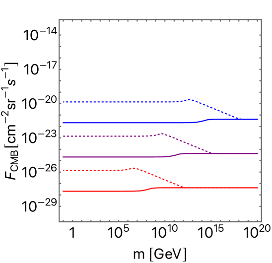
Figure 1: Threshold value of the MM flux beyond which the backreaction to the IGMFs becomes significant. The IGMF amplitude is varied as $B_{\mathrm{I}}=10^{-9}\,\mathrm{G}$ (blue), $10^{-12}\,\mathrm{G}$ (purple), $10^{-15}\,\mathrm{G}$ (red), with the correlation length $\lambda_{\mathrm{I}}>1/H_{0}$ (solid) and $\lambda_{\mathrm{I}}=1\,\mathrm{Mpc}$ (dashed). The MM charge is fixed to $g=g_{\mathrm{D}}$.

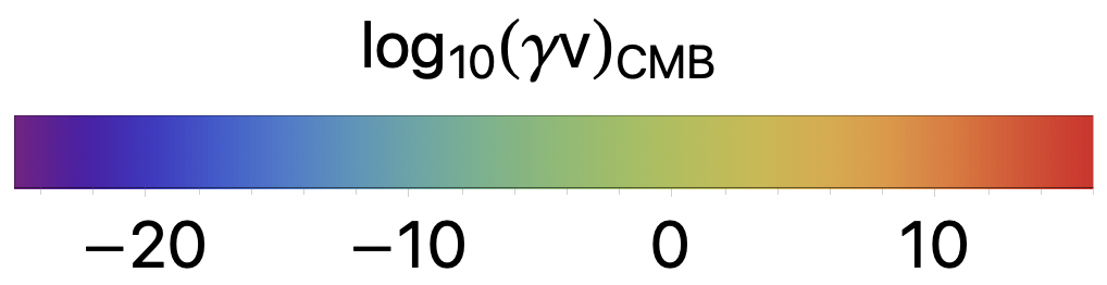
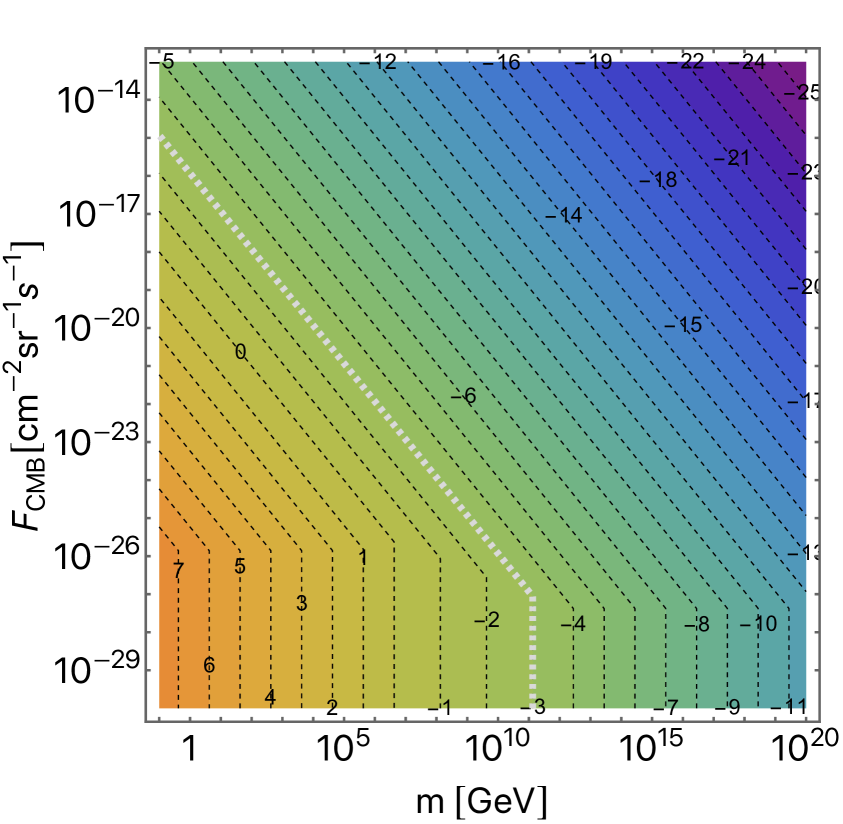
(a) $B_{\mathrm{I}}=10^{-15}\,\mathrm{G}$, $\lambda_{\mathrm{I}}=1\,\mathrm{Mpc}$.

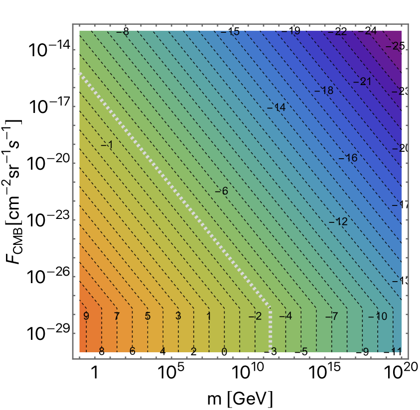
(b) $B_{\mathrm{I}}=10^{-15}\,G$, $\lambda_{\mathrm{I}}>1/H_{0}$.

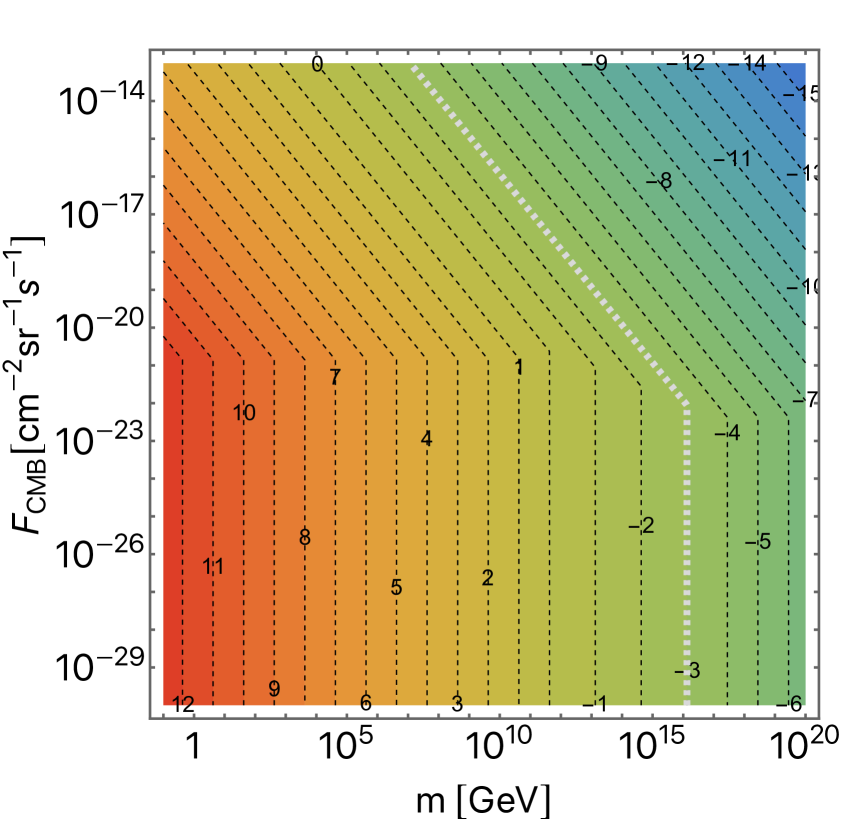
(c) $B_{\mathrm{I}}=10^{-10}\,G$, $\lambda_{\mathrm{I}}=1\,\mathrm{Mpc}$.

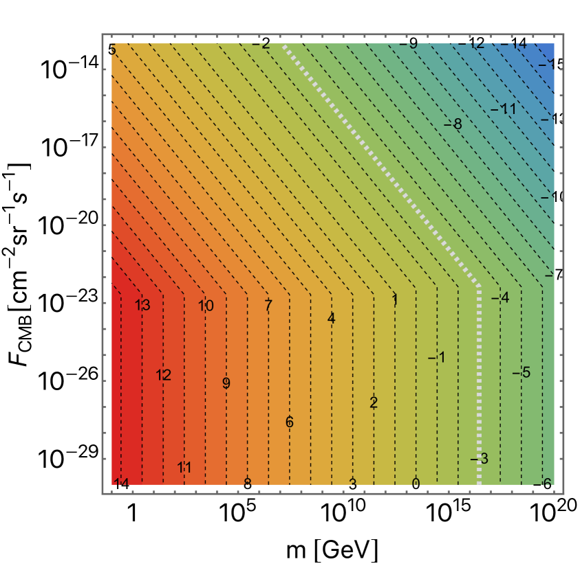
(d) $B_{\mathrm{I}}=10^{-10}\,G$, $\lambda_{\mathrm{I}}>1/H_{0}$.

Figure 2: Velocity of MMs accelerated in IGMFs, in the CMB rest frame. The contours show $\log_{10}(\gamma v)_{\mathrm{CMB}}$. The MM charge is fixed to $g=g_{\mathrm{D}}$, while the IGMF amplitude and coherence length are varied in each panel. Dashed gray lines highlight where $v_{\mathrm{CMB}}=10^{-3}$.

2.3 Monopole velocity in the CMB rest frame

In Figure 2 we show the value of $(\gamma v)_{\mathrm{CMB}}$ in Eq. (2.14) as a function of the MM mass and flux in the CMB rest frame. We display four combinations of the IGMF strength ($B_{\mathrm{I}}=10^{-15}\,\mathrm{G}$ and $10^{-10}\,\mathrm{G}$) and correlation length ($\lambda_{\mathrm{I}}=1\,\mathrm{Mpc}$ and $\lambda_{\mathrm{I}}>1/H_{0}$). The MM charge is fixed to $g=g_{\mathrm{D}}$. The values of $F_{\mathrm{CMB}}$ for which the contour lines of $(\gamma v)_{\mathrm{CMB}}$ are seen to bend correspond to the threshold $F_{\mathrm{BR}}$, which we showed in Figure 1. In the lower regions of each plot where $F_{\mathrm{CMB}}<F_{\mathrm{BR}}$, the backreaction on the IGMFs is negligible and we have $v_{\mathrm{CMB}}=v_{0}$, which is independent of the MM density. On the other hand in the upper regions where $F_{\mathrm{CMB}}>F_{\mathrm{BR}}$, the backreaction is significant and $v_{\mathrm{CMB}}=v_{\mathrm{max}}$; here the MM velocity depends on the flux but is independent of the IGMF coherence length, as shown in (2.16). The dashed gray line in the plot shows where $v_{\mathrm{CMB}}=10^{-3}$. This value is the same order as the peculiar velocity of the Milky Way, which will become important in the next section.

In Figure 3 we show $(\gamma v)_{\mathrm{CMB}}$ as a function of the MM mass for fixed values of the flux: $F_{\mathrm{CMB}}=10^{-30}\,\mathrm{cm}^{-2}\,\mathrm{sr}^{-1}\,\mathrm{s}^{-1}$ (solid lines) and $10^{-20}\,\mathrm{cm}^{-2}\,\mathrm{sr}^{-1}\,\mathrm{s}^{-1}$ (dashed). The IGMF strength and coherence length are taken as $B_{\mathrm{I}}=10^{-15}\,\mathrm{G}$ and $\lambda_{\mathrm{I}}=1\,\mathrm{Mpc}$ for the red lines, while $B_{\mathrm{I}}=10^{-10}\,\mathrm{G}$ and $\lambda_{\mathrm{I}}>1/H_{0}$ for the blue lines. The flux on the solid lines satisfy $F_{\mathrm{CMB}}<F_{\mathrm{BR}}$, and thus the MM velocity is set by $v_{0}$. On the other hand, the dashed lines have $F_{\mathrm{CMB}}>F_{\mathrm{BR}}$ and the MMs move at $v_{\mathrm{max}}$.

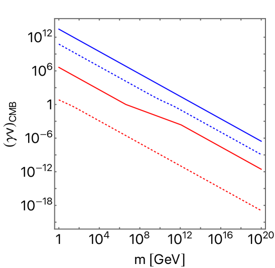
Figure 3: MM velocity in the CMB rest frame for fixed values of the MM flux: $F_{\mathrm{CMB}}=10^{-30}\,\mathrm{cm}^{-2}\,\mathrm{sr}^{-1}\,\mathrm{s}^{-1}$ (solid lines) and $10^{-20}\,\mathrm{cm}^{-2}\,\mathrm{sr}^{-1}\,\mathrm{s}^{-1}$ (dashed). The IGMF strength and coherence length are taken as $B_{\mathrm{I}}=10^{-15}\,\mathrm{G}$ and $\lambda_{\mathrm{I}}=1\,\mathrm{Mpc}$ for the red lines, while $B_{\mathrm{I}}=10^{-10}\,\mathrm{G}$ and $\lambda_{\mathrm{I}}>1/H_{0}$ for the blue lines. The MM charge is fixed to $g=g_{\mathrm{D}}$.

The above results show that, due to the acceleration in IGMFs, intermediate to low mass MMs can become relativistic. This remains true even when taking into account the backreaction on the IGMFs, albeit with a reduction in the MM velocity.

3 Modification of Parker bound

3.1 Parker bound

The abundance of MMs within the Milky Way Galaxy is constrained by the requirement that the MMs should not short out the Galactic magnetic fields [17, 18]. The upper bound on the MM flux inside the Milky Way thus obtained is commonly referred to as the Parker bound, and takes the form [25]

$$F_{\mathrm{MW}}\lesssim\mathrm{max.}\Biggl{\{} 10^{-16}\,\mathrm{cm}^{-2}\mathrm{sec}^{-1}\mathrm{sr}^{-1}\left(\frac{m\left(\gamma_{\mathrm{MW}}-1\right)}{10^{11}\,\mathrm{GeV}}\right)\left(\frac{g}{g_{\mathrm{D}}}\right)^{-2}\left(\frac{\lambda_{\mathrm{G}}}{1\,\mathrm{kpc}}\right)^{-1}\left(\frac{\tau_{\mathrm{gen}}}{10^{8}\,\mathrm{yr}}\right)^{-1},$$ (3.1)

$$10^{-16}\,\mathrm{cm}^{-2}\mathrm{sec}^{-1}\mathrm{sr}^{-1}\left(\frac{g}{g_{\mathrm{D}}}\right)^{-1}\left(\frac{B_{\mathrm{G}}}{10^{-6}\,\mathrm{G}}\right)\left(\frac{R}{\lambda_{\mathrm{G}}}\right)^{1/2}\left(\frac{\tau_{\mathrm{gen}}}{10^{8}\,\mathrm{yr}}\right)^{-1}\Biggr{\}}.$$

Here $\gamma_{\mathrm{MW}}$ is the Lorentz factor of the MMs in the rest frame of the Milky Way, $\lambda_{\mathrm{G}}$ is the coherence length of the Galactic magnetic field, $R$ is the size of the magnetic field region of the Galaxy, $\tau_{\mathrm{gen}}$ is the dynamo time scale for the amplification of the Galactic fields, and $B_{\mathrm{G}}$ is the mean Galactic field strength. One can further require the survival of the initial seed magnetic field of the Galaxy, the flux bound from which takes the same form except for that $B_{\mathrm{G}}$ is taken as the seed field strength [19].

The Parker bound applies to both MMs that are clustered with the Galaxy, and unclustered MMs which only pass through the Galaxy. However, with the typical parameters of the Galactic field shown as the reference values in the above equation, MMs with a Dirac charge can stay clustered until today only if they are ultraheavy as $m\gtrsim 10^{18}\,\mathrm{GeV}$ [18, 25]. As we are primarily interested in intermediate to low mass MMs which are significantly accelerated in IGMFs, in the following we focus on unclustered MMs.

The Parker bound uses the entire Galaxy as a MM detector, and consequently the bound depends on the MMs’ incident velocity on the Galaxy. The first line of (3.1) actually depends on $\gamma_{\mathrm{MW}}$, and in particular, the Parker bound becomes weaker for larger $\gamma_{\mathrm{MW}}$. This is because fast-moving MMs pass through the Galaxy while being minimally deflected by the Galactic field, hence do not effectively dissipate the magnetic energy. In the literature, the incident velocity has always been assumed to be $v_{\mathrm{MW}}\sim 10^{-3}$ (i.e. $\gamma_{\mathrm{MW}}-1\sim 10^{-6}$), as both the Milky Way’s peculiar velocity and the MMs’ gravitational infall velocity are of this order. However we have seen in the previous section that MMs can be accelerated to much larger velocities in the IGMFs. In the following, we study how the presence of IGMFs affect the Parker bound.

3.2 Monopole velocity in the Milky Way’s rest frame

The peculiar velocity of the Milky Way Galaxy with respect to the CMB rest frame, $v_{\mathrm{p}}\sim 10^{-3}$, sources a relative velocity between the cosmic MMs and the Galaxy. However if the MM velocity $v_{\mathrm{CMB}}$ obtained in the IGMFs is even larger, this would dominate the relative velocity. Therefore, the MM velocity in the rest frame of the Milky Way can be written as

$$v_{\mathrm{MW}}=\mathrm{max.}\left\{v_{\mathrm{p}},v_{\mathrm{CMB}}\right\}.$$ (3.2)

We also denote the incident flux of MMs on the Milky Way by $F_{\mathrm{MW}}=nv_{\mathrm{MW}}/4\pi$; this is equivalent to the MM flux inside the Milky Way from the conservation of the number of MMs. In Figure 2 we showed the combination of $m$ and $F_{\mathrm{CMB}}$ for which $v_{\mathrm{CMB}}\sim v_{\mathrm{p}}$ by the dashed gray line. On the left of the gray line where $v_{\mathrm{CMB}}>v_{\mathrm{p}}$, the quantities $v_{\mathrm{CMB}}$ and $F_{\mathrm{CMB}}$ are identical to $v_{\mathrm{MW}}$ and $F_{\mathrm{MW}}$, respectively. On the other hand, on the right of the gray line where $v_{\mathrm{CMB}}<v_{\mathrm{p}}$, the MM velocity in the Milky Way’s rest frame becomes $v_{\mathrm{p}}$. Therefore, contour plots of $(\gamma v)_{\mathrm{MW}}$ in the $m$-$F_{\mathrm{MW}}$ plane are the same as in Figure 2 except for that on the right of the gray dashed lines, $(\gamma v)_{\mathrm{MW}}$ is fixed to a constant value of $(\gamma v)_{\mathrm{p}}$.

3.3 Parker bound in the presence of intergalactic magnetic fields

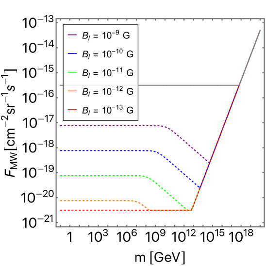
Figure 4: Galactic Parker bound and seed Galactic Parker bound in the presence of IGMFs with strength $B_{\mathrm{I}}\leq 10^{-9}\,\mathrm{G}$. The MM charge is fixed to $g=g_{\mathrm{D}}$. The Galactic Parker bound is not affected by the IGMFs and thus is shown by a single gray solid line. The seed Galactic Parker bound is affected, which is shown by dashed curves with different colors corresponding to different IGMF strengths. The Galactic field strength is taken as $B_{\mathrm{G}}=10^{-6}\,\mathrm{G}$, and the seed field as $B_{\mathrm{G}}=10^{-11}\,\mathrm{G}$, with the other parameters taken as $\lambda_{\mathrm{G}}=1\,\mathrm{kpc}$, $R=10\,\mathrm{kpc}$, $\tau_{\mathrm{gen}}=10^{8}\,\mathrm{yr}$. The curves overlap in the right part of the plot.

In Figure 4 we plot the Parker bound in Eq. (3.1), with the MM Lorentz factor $\gamma_{\mathrm{MW}}$ evaluated through Eq. (3.2). The MM charge is fixed to $g=g_{\mathrm{D}}$. The gray solid line shows the bound from the survival of Galactic fields with $B_{\mathrm{G}}=10^{-6}\,\mathrm{G}$, while the dashed curves are from seed fields with an assumed strength of $B_{\mathrm{G}}=10^{-11}\,\mathrm{G}$. The other Galactic parameters are fixed to $\lambda_{\mathrm{G}}=1\,\mathrm{kpc}$, $R=10\,\mathrm{kpc}$, $\tau_{\mathrm{gen}}=10^{8}\,\mathrm{yr}$, and $v_{\mathrm{p}}=10^{-3}$. The IGMF strength is varied between $B_{\mathrm{I}}=10^{-9}\,\mathrm{G}$ and $B_{\mathrm{I}}=10^{-13}\,\mathrm{G}$. IGMFs within this range do not affect the Galactic bound, which hence is shown by a single solid line. On the other hand, the seed bound is strongly affected by the presence of IGMFs; dashed lines of different colors correspond to different IGMF strength as shown in the plot legend. The Parker bounds for a fixed MM velocity of $v_{\mathrm{MW}}=10^{-3}$, as have been assumed in the literature, are reproduced for sufficiently weak IGMFs. The Galactic and seed bounds in the weak IGMF limit are shown respectively by the gray solid and red dashed curves. All the curves join at large masses, in other words, IGMFs modify the seed bound at intermediate to low masses. We also note that with the choice of parameters, the flux bounds are independent of the IGMF correlation length, as long as it is as large as $\lambda_{\mathrm{I}}\gtrsim 10^{-5}\,\mathrm{Mpc}$. This is because for values of $F_{\mathrm{MW}}$ that saturate the bound, $v_{\mathrm{MW}}$ is set either by $v_{\mathrm{p}}$ or $v_{\mathrm{max}}$, both of which do not depend on $\lambda_{\mathrm{I}}$. This can also be seen from Figures 4 and 1 showing that the upper bounds of $F_{\mathrm{MW}}$ are larger than the threshold value $F_{\mathrm{BR}}$ for the backreaction to the IGMFs to become relevant.

For MMs with large kinetic energies, the expression (3.1) for the Parker bound is set by the first line which explicitly depends on the kinetic energy. On the other hand for small kinetic energies, the bound is set by the second line which depends neither on the MM mass nor on the velocity. The presence of IGMFs thus modify the Parker bound if the MMs are accelerated to velocities larger than the Milky Way’s peculiar velocity, and further if the MM kinetic energy is sufficiently large such that the first line of the Parker bound applies.

For the choice of parameters in the plot, the upper bound on the flux from Galactic fields ($B_{G}=10^{-6}\,\mathrm{G}$) in the weak IGMF limit is of $F_{\mathrm{MW}}\sim 10^{-16}\,\mathrm{cm}^{-2}\mathrm{sec}^{-1}\mathrm{sr}^{-1}$ or larger. The threshold kinetic energy between the two expressions for the Parker bound is $m(\gamma_{\mathrm{MW}}-1)\sim 10^{11}\,\mathrm{GeV}$. For flux values saturating the bound, the energy that MMs acquire from IGMFs with $B_{I}\leq 10^{-9}\,\mathrm{G}$ is smaller than the threshold, which is why the Galactic bound is not altered by IGMFs. On the other hand, seed fields ($B_{G}=10^{-11}\,\mathrm{G}$) give an upper bound in the weak IGMF limit of $F_{\mathrm{MW}}\sim 10^{-21}\,\mathrm{cm}^{-2}\mathrm{sec}^{-1}\mathrm{sr}^{-1}$ or larger, with the threshold energy between the two expressions being $m(\gamma_{\mathrm{MW}}-1)\sim 10^{6}\,\mathrm{GeV}$. For the flux values, the energy can exceed the threshold with IGMFs of $B_{\mathrm{I}}\gtrsim 10^{-12}\,\mathrm{G}$, hence the seed Parker bound is modified.

In order to understand the behavior of the modified Parker bound, note that substituting Eq. (3.2) for $\gamma_{\mathrm{MW}}$ into the first line of Eq. (3.1) yields an upper limit which itself depends on the MM flux. In particular when $v_{\mathrm{MW}}=v_{\mathrm{max}}$ (i.e. $v_{\mathrm{p}}<v_{\mathrm{max}}<v_{0}$), one sees from Eq. (2.16) that $(\gamma v)_{\mathrm{MW}}\propto 1/\left(mF_{\mathrm{MW}}\right)$. For sufficiently small masses such that $v_{\mathrm{MW}}$ is relativistic, the kinetic energy scales as $m\gamma_{\mathrm{MW}}\propto 1/F_{\mathrm{MW}}$. Thus the first line of Eq. (3.1) yields an inequality of the form $F_{\mathrm{MW}}<\kappa/F_{\mathrm{MW}}$ where $\kappa$ is a factor that is independent of the MM mass and abundance. Solving this gives a flux bound $F_{\mathrm{MW}}<\kappa^{1/2}$, which is independent of the MM mass, as shown in the plot for the modified seed Parker bound at small masses. On the other hand for larger masses with nonrelativistic $v_{\mathrm{MW}}$, the kinetic energy scales as $mv_{\mathrm{MW}}^{2}/2\propto 1/mF_{\mathrm{MW}}^{2}$, and hence the first line of Eq. (3.1) becomes $F_{\mathrm{MW}}<\kappa/mF_{\mathrm{MW}}^{2}$. This gives a bound $F_{\mathrm{MW}}<(\kappa/m)^{1/3}$, which is stronger for larger masses, as is seen for the middle parts of the modified seed bounds in the plot.

Before ending this section, we should remark that if a sufficiently strong IGMF existed at the time of Galaxy formation, this could have grown during a protogalactic collapse into the currently observed Galactic field. In this scenario, the necessity for a seed Galactic field and the dynamo amplification is obviated, and hence the Parker bounds are modified; in particular, the seed Parker bound is nullified. Our findings indicate that even if a seed field coexisted with a strong IGMF and hence the seed Parker bound holds, it would be significantly relaxed due to the acceleration effect.

4 Conclusion

In light of the modern understanding of IGMFs, we have comprehensively analyzed the acceleration of MMs in the intergalactic space. We found in particular that MMs with intermediate to low masses are accelerated to relativistic velocities. The results are shown in Figure 2.

The MM acceleration in IGMFs has significant effects on direct and indirect searches. As one such example, we studied how the Galactic Parker bounds are modified for fast-moving MMs. Although it has been assumed in the literature that the initial MM velocity with respect to the Milky Way Galaxy is of the order of the peculiar velocity or the virial velocity of the Galaxy, this is not necessarily the case in the presence of IGMFs. We showed that the large MM velocity weakens the so-called extended Parker bound based on the survival of seed Galactic magnetic fields. On the other hand, the Parker bound from the present-day Galactic field is unaffected by IGMFs that are compatible with observations.

We also showed that if the cosmic flux of MMs is larger than the threshold values in Eqs. (2.17) or (2.18) (which are also illustrated in Figure 1), their backreaction on IGMFs is non-negligible. In this case the energy oscillates between the IGMFs and the MMs, and the oscillation-averaged MM velocity depends also on the MM density. Future developments in studies of IGMFs may be able to constrain such IGMF-MM oscillations, which will allow us to improve bounds on the MM flux.

This paper serves as a first step towards a complete understanding of MM acceleration in cosmic environments. An accurate knowledge of the velocity of MMs entering the Earth is crucial for interpreting the constraints from terrestrial detectors (e.g. [27, 28]) in terms of the MM mass. We will discuss the implications of acceleration effects for MM experiments in a companion work [29]. It would also be interesting to study relativistic MMs as a possible explanation of the recently claimed detection of an extremely high-energy cosmic ray [30]; see also the earlier papers [31, 14, 15, 32, 33] which studied similar ideas. Finally, we note that a cosmic population of relativistic MMs from IGMFs can serve as dark radiation, which may be further constrained from cosmological studies.

Appendix A Energy loss of fast monopoles in a nonrelativistic plasma

A MM traveling in a plasma loses its kinetic energy as it scatters off electrically charged particles. We evaluate the drag force experienced by the MM by following the procedure outlined in Section 14.2 of [34]. However here we consider the plasma to consist of nonrelativistic particles, and focus on cases where the MM velocity is much larger than the velocities of the individual plasma particles in the rest frame of the plasma.

We start in the rest frame of a MM. The magnetic field around the MM with charge $g$ is given by $\bm{B}=g\bm{r}/4\pi r^{3}$. (In this appendix $g$ is not necessarily the charge amplitude and thus can be negative.) Hence the equation of motion of a particle with electric charge $q$, velocity $\bm{u}$, and momentum $\bm{p}$ is

$$\frac{d\bm{p}}{dt}=\frac{qg}{4\pi}\frac{\bm{u}\times\bm{r}}{r^{3}}.$$ (A.1)

Integrating this yields the total change in the momentum of the particle scattered by the MM’s magnetic field. Focusing on small-angle scatterings, and hence ignoring the effect of the magnetic field on the particle’s trajectory, one obtains

$$\Delta p=\frac{\lvert qg\rvert}{4\pi}\int^{\infty}_{-\infty}dt\frac{u\sin\phi}{r^{2}}=\frac{\lvert qg\rvert}{2\pi b},$$ (A.2)

where $\phi$ is the angle between $\bm{r}$ and $\bm{u}$, and $b$ is the impact parameter. Upon moving to the far right-hand side we used $\sin\phi=b/r$, and $r=\sqrt{(ut)^{2}+b^{2}}$ with $t=0$ corresponding to when the distance between the particle and the MM is minimized. The scattering angle is $\theta=\Delta p/p$, with which the differential cross section is obtained as

$$\frac{d\sigma}{d\theta}=-2\pi b\frac{db}{d\theta}=\frac{(qg)^{2}}{2\pi p^{2}\theta^{3}}.$$ (A.3)

We assume that in the rest frame of the plasma, the MM velocity $\bm{v}$ has a much larger amplitude compared to the velocities of the individual plasma particles. Then in the MM rest frame, the particles can be considered to move with a universal velocity $\bm{u}=-\bm{v}$, and the scatterings with a collection of the particles induce the MM to experience a force,

$$\begin{split}\bm{F}&=\gamma n_{\mathrm{p}}\int d\theta\frac{d\sigma}{d\theta}u\bm{p}(1-\cos\theta)\\ &=\frac{C(qg)^{2}n_{\mathrm{p}}}{4\pi m_{\mathrm{p}}}\frac{\bm{u}}{u}.\end{split}$$ (A.4)

Here $m_{\mathrm{p}}$ represents the mass of the plasma particles, and $n_{\mathrm{p}}$ is the particle number density in the plasma rest frame; note that in the MM rest frame the number density is enhanced by the Lorentz factor $\gamma=1/\sqrt{1-v^{2}}$. The particle momentum is written as $\bm{p}=m_{\mathrm{p}}\gamma\bm{u}$, and we used that the average momentum transfer for a scattering with a small angle $\theta$ is $\bm{p}(1-\cos\theta)$. Upon moving to the second line, we have written the integral over small angles as

$$C=2\int d\theta\frac{1-\cos\theta}{\theta^{3}}\simeq\int\frac{d\theta}{\theta}=\ln\frac{\theta_{\mathrm{max}}}{\theta_{\mathrm{min}}}.$$ (A.5)

The upper limit of integration $\theta_{\mathrm{max}}$ can be set to unity as we are focusing on small-angle scatterings. The lower limit $\theta_{\mathrm{min}}$ arises from the fact that the above calculation based on single-particle scatterings breaks down if the impact parameter $b$ becomes larger than the mean free path of the particles in the plasma and/or the Debye length. Here we do not evaluate the detailed value of $\theta_{\mathrm{min}}$ since $\bm{F}$ is only logarithmically sensitive to it.

The expression for the drag force can be covariantized by noting that the force vector $\mathcal{F}^{\mu}$ should, in the MM rest frame, have spatial components matching with (A.4), along with a vanishing time component since the MM’s energy does not change. These are satisfied by a force vector with the form,

$$\mathcal{F}^{\mu}=-\frac{C(qg)^{2}n_{\mathrm{p}}}{4\pi m_{\mathrm{p}}}\frac{1}{v_{\mathrm{rel}}}\left\{\frac{\mathrm{u}^{\mu}}{\mathrm{u}_{\nu}\mathrm{v}^{\nu}}+\mathrm{v}^{\mu}\right\},$$ (A.6)

where we use $(-+++)$ for the metric signature, $\mathrm{v^{\mu}}$ is the four-velocity of the MM, $\mathrm{u^{\mu}}$ is the four-velocity of the plasma, and $v_{\mathrm{rel}}=\sqrt{1-(\mathrm{u}_{\nu}\mathrm{v}^{\nu})^{-2}}$ denotes the amplitude of the relative velocity between the MM and the plasma (in the MM rest frame, the spatial components of $\mathrm{u}^{\mu}$ reduce to $\gamma\bm{u}$, and $v_{\mathrm{rel}}=u$.)

The covariant equation of motion of a MM with mass $m$ in electromagnetic fields is given by

$$m\mathrm{v}^{\nu}\nabla_{\nu}\mathrm{v}^{\mu}=g\tilde{F}^{\mu\nu}\mathrm{v}_{\nu}+\mathcal{F}^{\mu},$$ (A.7)

with $\tilde{F}^{\mu\nu}$ being the dual electromagnetic field tensor. Taking a Minkowski metric and supposing that in the rest frame of the plasma there is only magnetic fields but no electric fields, then the equation of motion in the plasma rest frame reduces to

$$m\frac{d}{dt}(\gamma\bm{v})=g\bm{B}-\frac{C(qg)^{2}n_{\mathrm{p}}}{4\pi m_{\mathrm{p}}}\frac{\bm{v}}{v}.$$ (A.8)

Let us now compare the deceleration and acceleration terms in (A.8) in cosmic environments, by estimating their ratio:

$$\epsilon=\frac{1}{gB}\frac{C(qg)^{2}n_{\mathrm{p}}}{4\pi m_{\mathrm{p}}}.$$ (A.9)

As particles with smaller masses yield a larger drag force, here we focus on free electrons (instead of protons). In the intergalactic space, using the electron density in the intergalactic medium (IGM) $n_{e}\sim 1\,\mathrm{m}^{-3}$, the IGMF lower limit $B_{\mathrm{I}}\sim 10^{-15}\,\mathrm{G}$, and further taking $g=g_{\mathrm{D}}$ and $C\sim 1$, one finds $\epsilon\sim 10^{-10}$. In the Milky Way, considering instead the interstellar medium (ISM) with $n_{e}\sim 1\,\mathrm{cm}^{-3}$ and Galactic fields of $B_{\mathrm{G}}\sim 10^{-6}\,\mathrm{G}$ gives $\epsilon\sim 10^{-13}$. We thus see that both in the intergalactic space and the Milky Way, since the electron density is so small such that $n_{e}/m_{e}\ll B$, the acceleration of MMs in the magnetic fields completely dominates over the deceleration by scattering free electrons.

Let us comment on effects that we have not taken into account. Firstly, the above calculation is based on classical single-particle scatterings. A quantum field theory computation may give rise to corrections to the scattering cross section, especially in the ultrarelativistic regime. We also note that the picture of single-particle scatterings breaks down at distances larger than the Debye length, where plasma effects become important. These have been studied in [35, 36] for slow MMs, for which it was shown that the energy loss from plasma effects is typically not significantly larger than that from single-particle scatterings. Finally, we remark that MMs can further loose energy through ionization of neutral particles, atomic excitations, bremsstrahlung, electron-pair production, and photonuclear interactions; the last two processes become particularly important in the ultrarelativistic regime. (See e.g. [16] for a comprehensive study of energy-loss processes for MMs. A rough estimate of the interactions with neutral particles in the ISM is given in [25], according to which they are negligible for a wide range of parameters.) It would be important to study all these effects, in particular in the ultrarelativistic regime. We leave this for future work.

Before ending this appendix, we also estimate the energy loss of MMs through the emission of electromagnetic radiation. Using the Liénard formula (i.e. relativistic version of the Larmor formula), and exchanging the electric charge to magnetic, the energy loss per time of an accelerating MM is

$$P\sim g^{2}\gamma^{6}\left\{(\dot{\bm{v}})^{2}-(\bm{v}\times\dot{\bm{v}})^{2}\right\}=\frac{g^{4}B^{2}}{m^{2}},$$ (A.10)

where an overdot denotes a time-derivative. Upon moving to the far right-hand side, we have considered a MM accelerating along a homogeneous magnetic field and dropped the cross product, and also used the equation of motion (A.8) without the drag force term. The ratio between the radiative energy loss, and energy gain per time from the acceleration in the magnetic field, $gBv$ (here we take $g>0$), is thus

$$\delta\sim\frac{g^{3}B}{m^{2}v}.$$ (A.11)

For IGMFs of $B_{\mathrm{I}}=10^{-15}\,\mathrm{G}$, relativistic ($v\sim 1$) MMs with $g=g_{\mathrm{D}}$ give $\delta\sim 10^{-31}(1\,\mathrm{GeV}/m)^{2}$. For Galactic fields of $B_{\mathrm{G}}=10^{-6}\,\mathrm{G}$, this becomes $\delta\sim 10^{-22}(1\,\mathrm{GeV}/m)^{2}$. In either case, radiative emissions are negligible for relativistic MMs as long as the mass satisfies $m^{2}\gg g^{3}B$.

Appendix B Monopole-magnetic field oscillation

If MMs accelerated in magnetic fields do not dissipate their kinetic energy into the ambient plasma, they eventually return the energy to the magnetic fields. In this way the energy can move back and forth between the magnetic field and monopoles. However one would expect such oscillations to be subject to Landau damping, if the phase velocity of the magnetic field were smaller than the random velocity of the individual MMs [18].

In order to estimate the phase velocity, we start by considering a homogeneous one-dimensional system where the magnetic field has a component $B$ along a certain direction, and the MMs with charge $g$ ($>0$) have a velocity component $v$ along the same direction. (In this appendix, $B$ and $v$ are the not the amplitudes and thus can be negative.) Then by combining the MMs’ equation of motion, $m\,d(\gamma v)/dt=gB$, with the conservation of total energy density $\rho_{\mathrm{tot}}=nm\gamma+B^{2}/2$ where $n$ is the MM number density, one obtains an evolution equation for the magnetic field,

$$\frac{d^{2}B}{dt^{2}}+\Omega^{2}B=0.$$ (B.1)

Here $\Omega$ is the effective frequency taking the form:

$$\Omega=\frac{g}{\gamma^{3/2}}\left(\frac{n}{m}\right)^{1/2}.$$ (B.2)

This becomes time-independent for nonrelativistic MMs ($\gamma\simeq 1$), hence let us focus on this case for simplicity. Further supposing that inhomogeneous fields with a finite coherence length $\lambda$ also oscillate with this frequency, then the magnetic field’s phase velocity is obtained as $v_{\mathrm{ph}}=\lambda\Omega/2\pi$.

Galactic magnetic fields. The phase velocity of Galactic fields with coherence length $\lambda_{\mathrm{G}}$ is of

$$v_{\mathrm{ph}}\sim 10^{-5}\left(\frac{v_{\mathrm{MW}}}{10^{-3}}\right)^{-1/2}\left(\frac{F_{\mathrm{MW}}}{10^{-15}\,\mathrm{cm}^{-2}\mathrm{sec}^{-1}\mathrm{sr}^{-1}}\right)^{1/2}\left(\frac{g}{g_{\mathrm{D}}}\right)\left(\frac{m}{10^{18}\,\mathrm{GeV}}\right)^{-1/2}\left(\frac{\lambda_{\mathrm{G}}}{1\,\mathrm{kpc}}\right).$$ (B.3)

We have rewritten $n$ in terms of the MM flux in the rest frame of the Milky Way Galaxy (cf. below (3.2); however here we consider both clustered and unclustered monopoles), and set the reference value for the flux to the Galactic Parker limit at $m=10^{18}\,\mathrm{GeV}$ (cf. Figure 4). Note that MMs with a Dirac charge and mass $m\gtrsim 10^{18}\,\mathrm{GeV}$ can cluster with the Galaxy [18, 25]. Such clustered MMs obtain a virial velocity of $10^{-3}$, which is larger than the magnetic field’s phase velocity; hence the oscillation is expected to rapidly evaporate. The phase velocity can in principle become larger for smaller masses, however light MMs do not cluster and hence should pass through the Galaxy before (completely) returning the energy to the Galactic fields. A flux much larger than the Parker limit can also increase the phase velocity beyond the virial velocity, however [37] claimed that oscillating Galactic fields do not match with observations, and also that the inhomogeneity in the MM distribution further leads to the damping of the oscillations. For these reasons, one can derive the Parker bound without worrying about the possibility that the Galactic fields survive as oscillating fields.

Intergalactic magnetic fields. The phase velocity of IGMFs is of

$$v_{\mathrm{ph}}\sim 10^{-5}\,v_{\mathrm{CMB}}^{-1/2}\left(\frac{F_{\mathrm{CMB}}}{10^{-27}\,\mathrm{cm}^{-2}\mathrm{sec}^{-1}\mathrm{sr}^{-1}}\right)^{1/2}\left(\frac{g}{g_{\mathrm{D}}}\right)\left(\frac{m}{10^{10}\,\mathrm{GeV}}\right)^{-1/2}\left(\frac{\lambda_{\mathrm{I}}}{1\,\mathrm{Mpc}}\right).$$ (B.4)

Here we rewrote $n$ in terms of the flux in the CMB rest frame (cf. below (2.14)), and for its reference value used the flux threshold where the MM backreaction becomes relevant for IGMFs with $B_{\mathrm{I}}=10^{-15}\,\mathrm{G}$ at $m=10^{10}\,\mathrm{GeV}$ (cf. Figure 1). Note that the phase velocity increases for smaller $m$ and $v_{\mathrm{CMB}}$. MMs in the intergalactic space can obtain random velocities from scattering with the IGM and/or from gravitational potentials. However we expect these to be much smaller than the IGMF’s phase velocity, and hence in this paper we consider the IGMF-MM oscillations to survive.

Appendix C Monopole acceleration in intergalactic and galactic magnetic fields

MMs that cross the Earth are accelerated both by intergalactic and galactic magnetic fields. Depending on the amplitude and coherence length of IGMFs, and the MM number density and mass, one of the contributions is larger than the other. In this appendix we show the expected MM velocity at the Earth for different values of the MM mass and flux at the Earth, assuming a simple model for MM acceleration in Galactic fields.

Assuming Galactic magnetic fields with coherence length $\lambda_{\mathrm{G}}$, the velocities acquired by the MMs accelerated in Galactic magnetic fields is approximately:

$$\left(\gamma v\right)_{\mathrm{G}}\sim\frac{gB_{\mathrm{G}}\lambda_{\mathrm{G}}}{m}.$$ (C.1)

Therefore, the velocity of MMs on the Earth can be expressed as:

$$v_{\mathrm{Earth}}=\mathrm{max.}\left\{v_{\mathrm{G}},v_{\mathrm{MW}}\right\},$$ (C.2)

where $v_{\mathrm{MW}}$ is given by the expression in Eq. (3.2).

In Figure 5 we show the value of $v_{\mathrm{Earth}}$ in Eq. (C.2) as a function of the MM mass and flux at the Earth $F_{\mathrm{Earth}}=F_{\mathrm{MW}}$. In the figure we assume homogeneous IGMFs with $B=10^{-10}~{}\mathrm{G}$, and Galactic magnetic fields with amplitude $B_{\mathrm{G}}=10^{-6}~{}\mathrm{G}$ and $\lambda_{\mathrm{G}}=1~{}\mathrm{kpc}$. We also assume for the MM charge $g=g_{\mathrm{D}}$. We use the same color scheme of Figure 2. The plot shows three different behaviors of the MM velocity. In the upper region, the acceleration from Galactic fields is dominant over the acceleration from IGMFs. In this case, the value of the velocity is set by $v_{\mathrm{G}}$ and does not depend on the MM flux. In the central region, the velocity is set by $v_{\mathrm{MW}}$ and the backreaction on the IGMFs is non-negligible. In this case, the velocity depends on the MM flux in the CMB rest frame, and $F_{\mathrm{CMB}}=F_{\mathrm{Earth}}$. In the lower region, the velocity is still set by $v_{\mathrm{MW}}$ while the backreaction is negligible. Therefore, the velocity is independent of the MM flux. On the right part of the plot, the velocity is set by the peculiar velocity of the Milky Way, $v_{\mathrm{p}}\sim 10^{-3}$. The region excluded by the Galactic Parker bound is shown in gray.

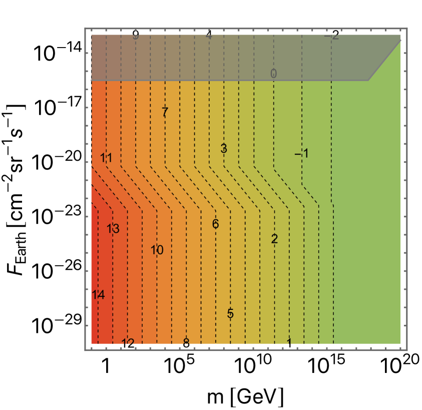
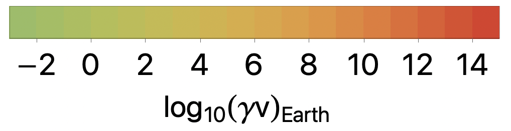
Figure 5: MM velocity after the acceleration due to IGMFs and Galactic magnetic fields with respect to the Milky Way rest frame. Here we assume IGMFs with $B_{\mathrm{I}}=10^{-10}~{}\mathrm{G}$ and $\lambda_{\mathrm{I}}>1/H_{0}$, and Galactic magnetic fields with $B_{\mathrm{G}}=10^{-6}~{}\mathrm{G}$ and $\lambda_{\mathrm{G}}=1~{}\mathrm{kpc}$. For the MM charge we use $g=g_{\mathrm{D}}$. The color scheme is the same as in Figure 2. The gray region is excluded by the Galactic Parker bound.

References

- [1] Paul Adrien Maurice Dirac. Quantised singularities in the electromagnetic field,. Proc. Roy. Soc. Lond. A, 133(821):60–72, 1931.
- [2] Gerard ’t Hooft. Magnetic Monopoles in Unified Gauge Theories. Nucl. Phys. B, 79:276–284, 1974.
- [3] Alexander M. Polyakov. Particle Spectrum in Quantum Field Theory. JETP Lett., 20:194–195, 1974.
- [4] Ya. B. Zeldovich and M. Yu. Khlopov. On the Concentration of Relic Magnetic Monopoles in the Universe. Phys. Lett. B, 79:239–241, 1978.
- [5] John Preskill. Cosmological Production of Superheavy Magnetic Monopoles. Phys. Rev. Lett., 43:1365, 1979.
- [6] F. Tavecchio, G. Ghisellini, L. Foschini, G. Bonnoli, G. Ghirlanda, and P. Coppi. The intergalactic magnetic field constrained by Fermi/LAT observations of the TeV blazar 1ES 0229+200. Mon. Not. Roy. Astron. Soc., 406:L70–L74, 2010.
- [7] A. Neronov and I. Vovk. Evidence for strong extragalactic magnetic fields from Fermi observations of TeV blazars. Science, 328:73–75, 2010.
- [8] Charles D. Dermer, Massimo Cavadini, Soebur Razzaque, Justin D. Finke, James Chiang, and Benoit Lott. Time Delay of Cascade Radiation for TeV Blazars and the Measurement of the Intergalactic Magnetic Field. Astrophys. J. Lett., 733:L21, 2011.
- [9] V. A. Acciari et al. A lower bound on intergalactic magnetic fields from time variability of 1ES 0229+200 from MAGIC and Fermi/LAT observations. Astron. Astrophys., 670:A145, 2023.
- [10] Ruth Durrer and Andrii Neronov. Cosmological Magnetic Fields: Their Generation, Evolution and Observation. Astron. Astrophys. Rev., 21:62, 2013.
- [11] Rafael Alves Batista and Andrey Saveliev. The Gamma-ray Window to Intergalactic Magnetism. Universe, 7(7):223, 2021.
- [12] Avery E. Broderick, Philip Chang, and Christoph Pfrommer. The Cosmological Impact of Luminous TeV Blazars I: Implications of Plasma Instabilities for the Intergalactic Magnetic Field and Extragalactic Gamma-Ray Background. Astrophys. J., 752:22, 2012.
- [13] Francesco Miniati and Andrii Elyiv. Relaxation of Blazar Induced Pair Beams in Cosmic Voids: Measurement of Magnetic Field in Voids and Thermal History of the IGM. Astrophys. J., 770:54, 2013.
- [14] Thomas W. Kephart and Thomas J. Weiler. Magnetic monopoles as the highest energy cosmic ray primaries. Astropart. Phys., 4:271–279, 1996.
- [15] C. O. Escobar and R. A. Vazquez. Are high-energy cosmic rays magnetic monopoles? Astropart. Phys., 10:197–202, 1999.
- [16] Stuart D. Wick, Thomas W. Kephart, Thomas J. Weiler, and Peter L. Biermann. Signatures for a cosmic flux of magnetic monopoles. Astropart. Phys., 18:663–687, 2003.
- [17] Eugene N. Parker. The Origin of Magnetic Fields. Astrophys. J., 160:383, 1970.
- [18] Michael S. Turner, Eugene N. Parker, and T. J. Bogdan. Magnetic Monopoles and the Survival of Galactic Magnetic Fields. Phys. Rev. D, 26:1296, 1982.
- [19] Fred C. Adams, Marco Fatuzzo, Katherine Freese, Gregory Tarle, Richard Watkins, and Michael S. Turner. Extension of the Parker bound on the flux of magnetic monopoles. Phys. Rev. Lett., 70:2511–2514, 1993.
- [20] Yoel Rephaeli and Michael S. Turner. The Magnetic Monopole Flux and the Survival of Intracluster Magnetic Fields. Phys. Lett. B, 121:115–118, 1983.
- [21] Dario Grasso and Hector R. Rubinstein. Magnetic fields in the early universe. Phys. Rept., 348:163–266, 2001.
- [22] Kandaswamy Subramanian. The origin, evolution and signatures of primordial magnetic fields. Rept. Prog. Phys., 79(7):076901, 2016.
- [23] Andrew J. Long and Tanmay Vachaspati. Implications of a Primordial Magnetic Field for Magnetic Monopoles, Axions, and Dirac Neutrinos. Phys. Rev. D, 91:103522, 2015.
- [24] Takeshi Kobayashi and Daniele Perri. Parker bound and monopole pair production from primordial magnetic fields. Phys. Rev. D, 106(6):063016, 2022.
- [25] Takeshi Kobayashi and Daniele Perri. Parker bounds on monopoles with arbitrary charge from galactic and primordial magnetic fields. Phys. Rev. D, 108(8):083005, 2023.
- [26] A. Kogut et al. Dipole anisotropy in the COBE DMR first year sky maps. Astrophys. J., 419:1, 1993.
- [27] R. Abbasi et al. Search for Relativistic Magnetic Monopoles with Eight Years of IceCube Data. Phys. Rev. Lett., 128(5):051101, 2022.
- [28] Alexander Aab et al. Search for ultrarelativistic magnetic monopoles with the Pierre Auger Observatory. Phys. Rev. D, 94(8):082002, 2016.
- [29] Daniele Perri, Kyrylo Bondarenko, Michele Doro, and Takeshi Kobayashi. in preparation.
- [30] R. U. Abbasi et al. An extremely energetic cosmic ray observed by a surface detector array. Science, 382:903–907, 2023.
- [31] N. A. Porter. The dirac monopole as a constituent of primary cosmic radiation. Nuovo Cimento, 16:958, 1960.
- [32] Veniamin Berezinsky, Pasquale Blasi, and Alexander Vilenkin. Ultrahigh-energy gamma-rays as signature of topological defects. Phys. Rev. D, 58:103515, 1998.
- [33] V. Berezinsky. Ultrahigh-energy cosmic rays from cosmological relics. Nucl. Phys. B Proc. Suppl., 87:387–396, 2000.
- [34] A. Vilenkin and E. P. S. Shellard. Cosmic Strings and Other Topological Defects. Cambridge University Press, 7 2000.
- [35] A. J. S. Hamilton and C. L. Sarazin. Deceleration of Grand Unified Theory monopoles in a plasma. Astrophys. J., 274:399–407, 1983.
- [36] N. Meyer-Vernet. Energy loss by slow magnetic monopoles in a thermal plasma. Astrophys. J., 290:21–23, 1985.
- [37] Eugene N. Parker. Magnetic Monopole Plasma Oscillations and the Survival of Galactic Magnetic Fields. Astrophys. J., 321:349, 1987.