How Network Topology Affects the Strength of Dangerous Power Grid Perturbations

Abstract

Reasonably large perturbations may push a power grid from its stable synchronous state into an undesirable state. Identifying vulnerabilities in power grids by studying power grid stability against such perturbations can aid in preventing future blackouts. We use two stability measures — stability bound, which deals with a system’s asymptotic behaviour, and survivability bound, which deals with a system’s transient behaviour, to provide information about the strength of perturbations that destabilize the system. Using these stability measures, we have found that certain nodes in tree-like structures have low asymptotic stability, while nodes with a high number of connections generally have low transient stability.

• December 2023

Keywords: power grids, probabilistic methods, network dynamics, stability of dynamical systems, coupled oscillator networks,

1 Introduction

Power grids are critical infrastructures that underpin the functioning of modern society. Failures in these systems have resulted in large-scale blackouts that have left millions of people without electricity [1, 2, 3]. In recent times, grid expansion, modernization, and decentralization have been promoting rapid change to existing power grid infrastructure [4, 5, 6]. Thus, as power grids are becoming increasingly more complex, it is important to ensure they are resilient to various perturbations in order to prevent future blackouts.

During normal operation, all parts of a power grid function at the same frequency [7]. This state is called the grid’s synchronous state. Perturbations such as a line being switched off or the power balance of the grid not being met may result in a cascading failure that causes large parts of the grid to desynchronize [8, 9, 10]. As perturbations affecting power grids can be reasonably large, linear stability analysis by means of evaluating the eigenvalues of the Jacobian matrix at an equilibrium point or the master stability function [11] cannot be employed as a measure of grid stability against such perturbations.

To quantify the stability of dynamical systems, such as power grids, against reasonably large perturbations, several non-local stability measures have been proposed [12, 13, 14, 15, 16, 17, 18]. Among these, a popular stability measure, known as basin stability [12], relates to the fraction of phase space that forms the basin of attraction of the desirable attractor. In the context of power grids, the desirable attractor corresponds to the grid’s stable synchronous state. Basin stability has been used extensively in the study of power grid stability [19, 20, 21, 22, 23, 24, 25, 26].

Basin stability deals with the asymptotic behaviour of a system. In addition to the asymptotic behaviour, the transient behaviour is particularly relevant when dealing with power grids. Power grids operate within certain frequency bounds, and control mechanisms are triggered when a perturbation causes the grid to operate out of the set frequency bound. Such perturbations are undesirable for the system. A stability measure called survivability has been proposed to quantify the transient stability of dynamical systems [13]. The set of states that do not leave a given desirable region of the phase space within a given time is called the basin of survival, and survivability is the fraction of states that are part of the system’s basin of survival. Thus, survivability measures a system’s ability to keep perturbations within a desirable region. Survivability, like basin stability, has been used to study power grid stability [13, 22, 27].

Basin stability and survivability are both volume-based measures of stability as they are related to the volume of the basin of attraction and the volume of the basin of survival, respectively. For power grids, the basin of attraction of the synchronous state can be very distorted [28]. It is possible that a stronger perturbation is safe for the system, but a weaker one is not. Hence, it is crucial to understand the magnitude of perturbations that are dangerous for the system. The volume-based stability measures fail to capture this. However, a distance-based stability measure called stability bound [29] captures this aspect. Stability bound is a stability quantifier that provides a bound to the strength of safe perturbations based on the system’s asymptotic behaviour. Analogous to stability bound, we propose a distance-based stability quantifier called survivability bound that provides a bound to the strength of safe perturbations based on the system’s transient behaviour.

Using these distance-based stability measures, we study how network topology affects power grid stability. We find that certain nodes which are part of tree-like network structure have a low stability bound, indicating that these nodes require the least perturbation strength to cause permanent grid synchrony loss. On the other hand, we find that nodes with a high number of connections have a low survivability bound, indicating that these nodes require the least perturbation strength to cause undesirable transients in the system, which do not necessarily lead to loss of grid synchrony.

This paper is organized as follows. The power grid model, methods of stability quantification, and a classification of network nodes are presented in section 2. Section 3 describes the results, and section 4 concludes the work.

2 Methods

2.1 Power grid model

We use a complex network representation to model power grids with generators and consumers as nodes and transmission lines as edges. Generators and consumers are modelled as synchronous machines that follow the swing equation [7]. The equations that describe the dynamics of the grid are [30]

$$\dot{\theta_{i}} = \omega_{i},$$ (1a)

$$I_{i}\dot{\omega_{i}} = -\gamma_{i}\omega_{i}+\bar{P_{i}}-\sum^{N}_{j=1}T_{ij}\sin(\theta_{i}-\theta_{j}),$$ (1b)

where $\theta_{i}$ and $\omega_{i}$ are the phase angle and the angular velocity of the synchronous machine at the $i^{\rm th}$ node of the power grid network in a frame rotating at the grid frequency. $I_{i}$ is the inertia at the $i^{\rm th}$ node, $\gamma_{i}$ is the damping at the $i^{\rm th}$ node, and $\bar{P}_{i}$ is proportional to the net power generated or consumed at the $i^{\rm th}$ node. $T_{ij}$ is the transmission capacity between node $i$ and node $j$. If node $i$ and node $j$ are not connected, then $T_{ij}=0$.

If all nodes have equal inertia ($I_{i}=I$), damping ($\alpha_{i}=\alpha$), then,

$$\dot{\theta_{i}} = \omega_{i},$$ (1ba)

$$\dot{\omega_{i}} = -\alpha\omega_{i}+P_{i}-\sum^{N}_{j=1}K_{ij}\sin(\theta_{i}-\theta_{j}),,$$ (1bb)

where $\alpha=\gamma/I$, $P_{i}=\bar{P_{i}}/I$, $K_{ij}=T_{ij}/I$.

In this paper, we use the simplified differential equations described by equations 1ba and 1bb to model power grids. Each node in the network has two corresponding dynamical variables — a phase angle and a frequency. The fixed point of these equations correspond to the stable synchronous state of the grid. In this state, the $i^{\rm th}$ node has a phase $\theta_{i}^{s}$ and frequency $0$.

2.2 Stability bound

Consider an $N$ dimensional dynamical system with a phase space $X$. The set $\mathcal{A}$ is the system’s desirable attractor. This attractor has a basin of attraction $\mathcal{B}$. We consider a finite subset of the phase space $X^{0}\subseteq$ X, representing the extent to which perturbations can push the system.

The basin stability of the attractor $\mathcal{A}$, defined in a region $X^{P}$ is the fraction of states in the region $X^{P}$ contained in the attractor’s basin of attraction $\mathcal{B}$. The basin stability, assuming a uniform distribution of perturbations, is defined as [12, 19, 22]

$$\beta(X^{P})=\frac{\textnormal{Vol}(\mathcal{B}\cap X^{P})}{\textnormal{Vol}(X^{P})}$$ (1bc)

Thus, basin stability measures the probability that a perturbation in the region $X^{P}$ causes the system to return to its desirable attracting state.

Let ${X^{D}(d)}$ be the set of states within a distance $d$ from the attractor $\mathcal{A}$ that lie in the set $X^{0}$, i.e.,

$${X^{D}}(d)=\{x\in{X^{0}}\>|\>\textnormal{dist}(x,\mathcal{A})<d\}$$ (1bd)

where $\textnormal{dist}(x,\mathcal{A})$ is the distance of the state $x$ to the attractor $\mathcal{A}$.

${D}$ is the set of distances at which the corresponding basin stability is less than a basin stability tolerance $t_{\beta}$. Thus,

$${D_{\beta}}=\{d\in(0,d_{\textnormal{max}}]\>|\>\beta({X^{D}}(d))<t_{\beta}\}$$ (1be)

where $t_{\beta}\in(0,1]$ is a predefined basin stability tolerance, and $d_{\textnormal{max}}$ is the maximum distance we would like to consider.

The stability bound of the attractor $\mathcal{A}$ is defined as [29]

$$\bar{\beta}=\cases{\textnormal{inf}(D_{\beta})&if $D_{\beta}\neq\phi$\\ d_{\textnormal{max}}&otherwise\\ }$$ (1bf)

Thus, the stability bound is the minimum distance at which the corresponding basin stability is less than the tolerance $t_{\beta}$.

Single-node stability bound is defined as the stability bound with perturbations conditioned to a single network node starting from the initial attracting state. For a power grid, we consider a perturbation to $\theta_{i}$ as a single-node perturbation at node $i$. If single-node perturbations occur in the region $X^{sn}$, such that $\theta_{i}\in X^{sn}$ is a single-node perturbation at the $i^{\rm th}$ node; then the single-node stability bound of node $i$ of the grid network is the stability bound defined in the region.

$$X_{i}^{0}=\{(\theta,\omega)\in X|(\theta_{i}\in X^{sn}\land\omega_{i}=0\land(\forall j\neq i:\theta_{j}=\theta^{s}_{j}\land\omega_{j}=0)\}$$ (1bg)

where $\theta=(\theta_{1},\theta_{2},...,\theta_{N})$ and $\omega=(\omega_{1},\omega_{2},...,\omega_{N})$

Basin stability is estimated using a Monte Carlo simulation. In the region ${X^{P}}$, a number of initial conditions, $n$, are sampled from a uniform distribution. If the number of initial conditions that converge to the attractor $\mathcal{A}$ is $n_{\beta}$, then the estimated basin stability of the attractor is

$$\hat{\beta}(X^{P})=\frac{n_{\beta}}{n}$$ (1bh)

The standard error $e$ associated with the basin stability computation is always less than equal to ${0.5}/{\sqrt{n}}$.

To compute the stability bound, the basin stability $\hat{\beta}(X^{D}(d))$ is computed from $d=d_{\textnormal{max}}$ to $d=d_{0}$, using $n$ samples for every basin stability estimation. $d_{0}$ is the largest distance such that $\hat{\beta}({X^{D}}(d_{0}))=1$. For $\hat{\beta}(X^{D}(d))<t_{\beta}$, the values of $d$ are noted and added to a set ${D_{\beta}}$. The stability bound is computed using equation 1bf. Refer to the paper by Alvares et al. [29] for a detailed computation procedure.

At the distance $d$, the corresponding estimate of basin stability within one standard deviation error is reported in the confidence interval $[\hat{\beta}(X^{D}(d))-e,\hat{\beta}(X^{D}(d))+e]$. Due to the uncertainty in the estimation of basin stability, the stability bound can also be reported in a confidence interval. The stability bound computed using the lower (upper) bound of the confidence interval of the estimated basin stability corresponds to the lower (upper) bound of the confidence interval of the estimated stability bound.

2.3 Survivability bound

Consider an $N$ dimensional dynamical system with a phase space $X$ and a desirable attractor $\mathcal{A}$. We consider a finite subset of the phase space $X^{0}\subseteq$ X, representing the extent to which perturbations can push the system.

Suppose the system has a desirable region $X^{+}\subseteq X$ of the phase space. A perturbation is considered safe if it does not leave the desirable region in a finite time $t$. Let $X^{S}_{t}$ be the set of points in $X^{P}$ that do not leave the desirable region $X^{+}$ in the time $t$. Assuming a uniform distribution of perturbations in the region $X^{P}$, survivability is defined as [13, 22]

$$\sigma(X^{P})=\frac{\textnormal{Vol}(X_{t}^{S})}{\textnormal{Vol}(X^{0})}$$ (1bi)

Survivability, thus, represents the probability that a perturbation in the region $X^{P}$ remains in the desirable region.

Consider ${D_{\sigma}}$ the set of distances at which the corresponding survivability is less than a survivability tolerance $t_{\sigma}$.

$${D_{\sigma}}=\{d\in(0,d_{\textnormal{max}}]\>|\>\sigma({X^{D}}(d))<t_{\sigma}\}$$ (1bj)

where $t_{\sigma}\in(0,1]$ is a predefined survivability tolerance, $d_{\textnormal{max}}$ is the maximum distance we would like to consider, and $X^{D}(d)$ is given by equation (1bd).

We define the survivability bound of the attractor ${\mathcal{A}}$ as

$$\bar{\sigma}=\cases{\textnormal{inf}(D_{\sigma})&if $D_{\sigma}\neq\phi$\\ d_{\textnormal{max}}&otherwise\\ }$$ (1bk)

Thus, survivability bound as the minimum distance at which the corresponding survivability is less than the tolerance $t_{\sigma}$.

In the case of the power grids, the desirable region is defined to be

$$X^{+}=\{(\theta,\omega)\in X|\forall i:-\pi<\theta_{i}<\pi\land-\omega^{+}<\omega_{i}<\omega^{+}\}$$ (1bl)

where $\theta=(\theta_{1},\theta_{2},...,\theta_{N})$ and $\omega=(\omega_{1},\omega_{2},...,\omega_{N})$ and $w^{+}$ is a set bound to the frequency fluctuation.

If single-node perturbations occur in the region $\theta_{i}\in X^{sn}$, then the single-node survivability bound of node $i$ is the survivability bound defined in the phase space region given by equation (1bg).

Survivability is estimated using a Monte Carlo simulation. In the region ${X^{P}}$, a number of initial conditions, $n$, are uniformly sampled. If the number of initial conditions that converge to the attractor $\mathcal{A}$ is $n_{\sigma}$, then the estimated survivability is

$$\hat{\sigma}=\frac{n_{\sigma}}{n}$$ (1bm)

The standard error $e$ associated with the survivability estimation is always less than equal to ${0.5}/{\sqrt{n}}$. The survivability bound is computed using the same procedure used to compute the stability bound.

2.4 Quantifying the strength of power grid perturbations

Stability bound and survivability bound rely on a notion of distance between a perturbed state and the attractor. This distance is indicative of the strength of perturbation. Distance in the phase space of a dynamical system can be quantified in various ways, ranging from standard Euclidean distance to the energy difference between the two states [29, 31]. For the distance of a perturbation from the synchronous state to have a physical meaning, we quantify it by defining an energy function that is related to the energy change of the system due to the perturbation.

Note that we have used a simplified power grid model given by equations 1ba and 1bb with the inertia at all nodes being the same and quantities such as torque and energy that we refer to are normalized by inertia.

Consider a perturbation in the phase angle $\theta_{i}$ at the node $i$ from the stable state value of $\theta_{i}=\theta_{i}^{s}$ to $\theta_{i}=\theta_{i}^{p}$. It can be that either $\theta_{i}^{s}<\theta_{i}^{p}$ or $\theta_{i}^{s}>\theta_{i}^{p}$. We assume that no energy is transferred back from the system in the process of perturbing $\theta_{i}$. In, the journey from $\theta_{i}^{s}$ to $\theta_{i}^{p}$, the external torque required is

$$\tau(\theta_{i})=\cases{-\textnormal{min}\{0,\frac{d^{2}\theta_{i}}{dt^{2}}\}&if $\theta_{i}^{p}>\theta_{i}>\theta_{i}^{s}$\\ -\textnormal{max}\{0,\frac{d^{2}\theta_{i}}{dt^{2}}\}&if $\theta_{i}^{p}<\theta_{i}<\theta_{i}^{s}$}$$ (1bn)

Additionally, we also assume that the perturbation is made at the synchronous grid frequency, which makes $w_{i}=0$. The torque required for this is

$$\tau(\theta_{i})=\cases{-\textnormal{min}\{0,(P_{i}-\sum^{N}_{j=1}K_{ij}\sin(\theta_{i}-\theta_{j}))\}&if $\theta_{i}^{p}>\theta_{i}>\theta_{i}^{s}$\\ -\textnormal{max}\{0,(P_{i}-\sum^{N}_{j=1}K_{ij}\sin(\theta_{i}-\theta_{j}))\}&if $\theta_{i}^{p}<\theta_{i}<\theta_{i}^{s}$}$$ (1bo)

The work $W(\theta_{i}^{s},\theta_{i}^{p})$ done in moving from $\theta_{i}^{s}$ to $\theta_{i}^{p}$ is

$$W(\theta_{i}^{s},\theta_{i}^{p})=\int^{\theta_{i}^{p}}_{\theta_{i}^{s}}\tau(\theta_{i})\>d\theta_{i}$$ (1bp)

The perturbation from $\theta_{i}^{s}$ to $\theta_{i}^{p}$ can happen through two different paths. For $\theta_{i}^{p}>\theta_{i}^{s}$, the two possible paths are $\theta_{i}^{s}\rightarrow\theta_{i}^{p}$ and $\theta_{i}^{s}\rightarrow-2\pi+\theta_{i}^{p}$. For $\theta_{i}^{p}<\theta_{i}^{s}$, the two possible paths are $\theta_{i}^{s}\rightarrow\theta_{i}^{p}$ or $\theta_{i}^{s}\rightarrow 2\pi+\theta_{i}^{p}$. We define energy $E(\theta_{i}^{p})$ as the energy of the perturbation from $\theta_{i}^{s}$ to $\theta_{i}^{p}$ along the path corresponding to the least energy change. Thus,

$$E(\theta_{i}^{p})=\cases{\textnormal{min}\{W(\theta_{i}^{s},\theta_{i}^{p}),\>W(\theta_{i}^{s},-2\pi+\theta_{i}^{p})\}&if $\theta_{i}^{p}>\theta_{i}^{s}$\\ \textnormal{min}\{W(\theta_{i}^{s},\theta_{i}^{p}),\>W(\theta_{i}^{s},2\pi+\theta_{i}^{p})\}&if $\theta_{i}^{p}<\theta_{i}^{s}$}$$ (1bq)

The distance between the perturbed state and the attractor is taken as the energy change of the system corresponding to a perturbation in the phase $\theta_{i}^{p}$ at node $i$ from the initial stable state. Thus,

$$\textnormal{dist}(x_{i}^{p},\mathcal{A})=E(\theta_{i}^{p})$$ (1br)

where $x_{i}^{p}=(\theta_{1}^{s},\>\theta_{2}^{s},\>...,\>\theta_{i}^{p},\>...,\>\theta_{N}^{s},\>0,\>0,\>...,\>0,\>...,\>0)$

2.5 Network motifs

J. Nitzbon et al. [22] have identified some important network motifs relevant to studying power grid stability. These network motifs are described below.

Consider a graph $G=(V,E)$ with vertices $V$ and edges $E$. $G=(V,E)$ is a tree if it is connected and has no cycles. $T^{\prime}=(V^{\prime},E^{\prime})$ is a tree-shaped part of $G$ if it is an induced subgraph of $G$, is a tree and is maximal with the property that there is exactly one node $r\in V^{\prime}$ that has at least one neighbour in $G-T^{\prime}$. The node $r$ of $T^{\prime}$ is called a root node ($R$). The union of all tree-shaped parts of the graph $G$ is called the forest $T$ of the graph $G$. For a tree-shaped part, the depth of node $x$ is the length of the shortest path from node $x$ to the root node.

Nodes that do not belong to the forest part $T$ are called bulk nodes ($B$). Nodes that belong to the forest part and are not root nodes are called non-root nodes. Non-root nodes that have a degree greater than one are called inner tree nodes ($I$). Non-root nodes that have a degree of one are called leaves. Leaves that have a depth of more than one are proper leaves ($P$). Leaves that have a depth one are called sprouts. Sprouts with an average neighbour degree less than six are called sparse sprouts ($S_{s}$). Sprouts with an average neighbour degree of more than five are called dense sprouts ($S_{d}$). Fig. 1 shows a network with nodes classified as described above.

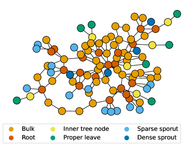
Figure 1: A network with nodes classified as bulk nodes, root nodes, inner tree nodes, proper leaves, sparse sprouts, and dense sprouts.

Besides these network motifs, betweenness centrality is important in understanding vulnerable power grid structures. Betweenness centrality measures the importance of a node in a network based on how many shortest paths pass through it. The betweenness centrality of node $i$ in a network is defined as [32]

$$b_{i}=\sum_{j\neq i,k\neq i,k>j}\frac{\sigma_{jk}^{i}}{\sigma_{jk}}$$ (1bs)

where $\sigma_{jk}^{i}$ is the number of shortest paths from node $j$ to node $k$ which pass through node $i$, and $\sigma_{jk}$ is the number of shortest paths which pass from node $j$ to node $k$.

3 Results

We use a random network generator model proposed by Schultz et al. [33] to generate realistic power grid networks to study the effect of network topology on power grid stability. The parameters chosen for this model are $N_{0}=1$, $p=1/5$, $q=3/10$, $s=1/3$, $t=1/10$. $50$ such networks, each consisting of $100$ nodes, were generated. In each network, half of the nodes were taken to be generators, and half of the nodes were taken to be consumers. Grid networks were modelled using equations 1ba and 1bb, with the following parameters: $K=6$ for every transmission line, $\alpha=0.1$ for every node, $P=1$ for every generator, and $P=-1$ for every consumer. One unit of time in the differential equations corresponds to $0.25$ s. Using this ensemble of grid networks, we investigate the single-node stability bound and the single-node survivability bound for every node of all the networks.

Deviations in the grid frequency of power grids are generally kept within $\pm 1$ Hz. A deviation of $\pm 1$ Hz in the frequency corresponds to a $\omega\approx\pm 1.57$ in the units we have used. The desirable region’s frequency bound $\omega^{+}$ is chosen to be $\omega^{+}=1$. This corresponds to an allowed frequency deviation of $\pm 0.64$ Hz. The region $X^{sn}=[-\pi,\pi]$ represents single-node perturbations in the phase. The single-node stability bound and single-node survivability bound of node $i$ in a network are computed in the region $X_{i}^{0}$ given by equation (1bg) for single-node perturbations in the region $X^{sn}$. Stability bound and survivability bound are computed using tolerances $t_{\beta}=0.95$ and $t_{\sigma}=0.95$, respectively, and the maximum perturbation distance limit is set to $d_{\rm max}=50$. For all basin stability and survivability computations, $n=200$ initial conditions were used, and every initial condition was evolved for time $t=100$. Numerically, a perturbation is counted to be in the basin of attraction if $|\omega_{i}|<1\>\forall i$ at $t=100$.

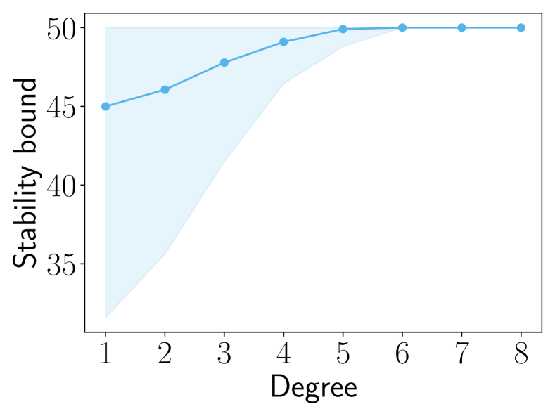
(a)

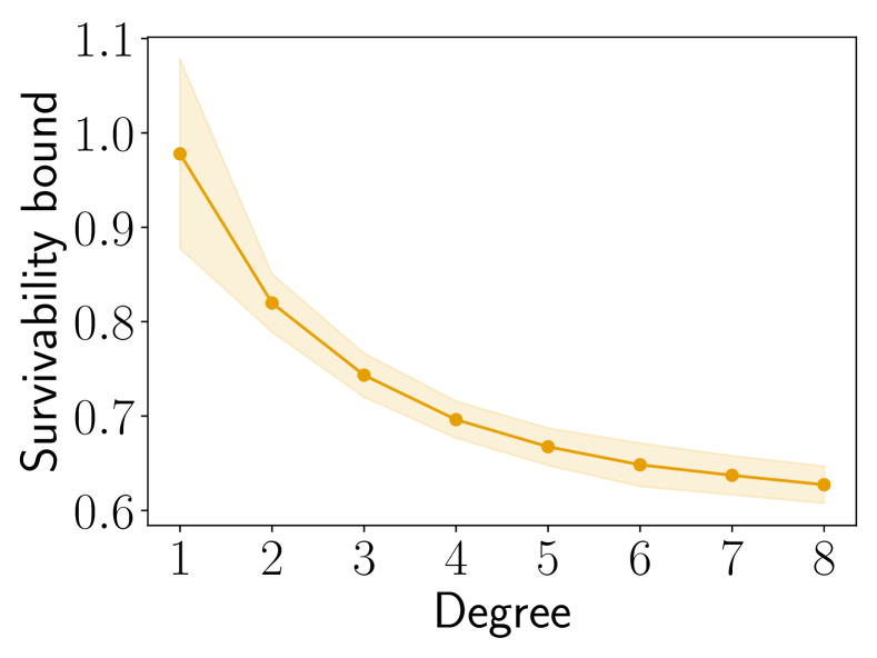
(b)

Figure 2: The dependence of single-node stability on degree. (a) Stability bound versus degree. (b) Survivability bound versus degree. The dots show the average value, and the shaded region indicates the error corresponding to $\pm 1$ standard deviation

Fig. 2 shows the relationship between degree and single-node stability. Fig. 2(a) shows that nodes with a lower degree have lower stability bound values. In contrast, survivability shows a negative correlation with a node’s degree, with nodes with a high degree being the least stable (Fig. 2(b)).

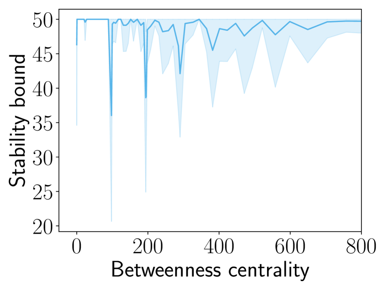
(a)

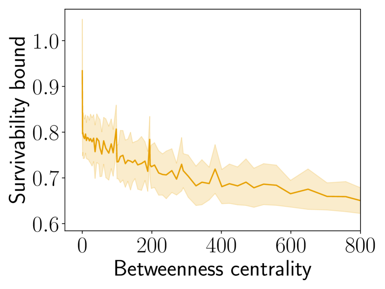
(b)

Figure 3: The dependence of single-node stability on betweenness centrality. (a) Stability bound versus betweenness centrality. (b) Survivability bound versus betweenness centrality. The line shows the average trend, and the shaded region indicates the error corresponding to $\pm 1$ standard deviation

Fig. 3 shows how single-node stability is related to betweenness centrality. In Fig. 3(a), marked dips in the stability bound are observed corresponding to betweenness centrality values of $N-2$, $2N-6$, and $2N-5$ (Here, $N=100$ — the number of nodes in each network). These dips correspond to nodes inside dead ends and dead trees [19], which can be broadly classified as inner leave nodes. A slight dip in the betweenness centrality of 0 is also observed, corresponding to nodes with a degree of one. Survivability bound does not show such dips and shows a negative correlation with betweenness centrality (Fig. 3(b)).

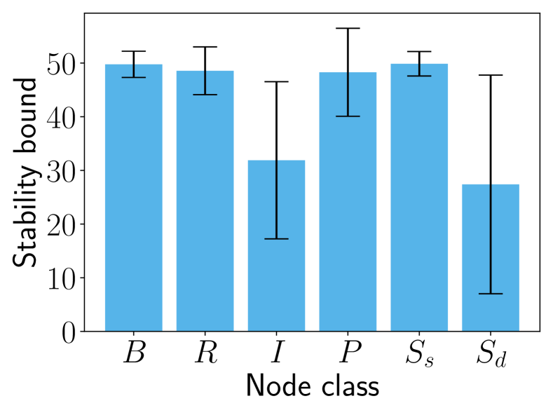
(a)

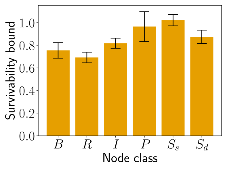
(b)

Figure 4: Bar graph showing the average single-node stability for each node class. (a) Stability bound for each node class. (b) Survivability bound for each node class. The black line indicates the range corresponding to $\pm 1$ standard deviation.

Fig. 4 shows the average single-node stability values for the different classes of nodes. Nodes with a degree of one have been seen to have low stability bound values (Fig. 2(a)). However, these nodes can be further divided into proper leaves, sparse sprouts and dense sprouts. In Fig. 4(a), we observe that dense sprouts are the least stable nodes out of all the nodes with a degree of one. Additionally, Fig. 4(a) shows that inner tree nodes have low stability bound values, as already evident from the dips at characteristic betweenness centrality values in Fig. 3(a). In Fig. 4(b), we observe that root nodes and bulk nodes have the lowest survivability bound values. These nodes are in the interior of networks and are thus generally well connected. This agrees well with the fact that survivability bound is negatively correlated with a node’s degree (Fig. 2(b)).

4 Conclusion

We have developed and employed asymptotic and transient stability measures to assess the magnitude of dangerous power grid perturbations. A perturbation stronger than a node’s stability bound can be devastating for the grid, and it can result in total grid synchrony loss. On the other hand, a perturbation stronger than a node’s survivability bound might be undesirable for the grid as it momentarily pushes node frequencies out of the desirable operation region without necessarily pushing the grid permanently out of synchrony.

Through the study of the single-node stability of an ensemble of synthetic power grids, we have identified vulnerable local network properties of power grids. We have found that inner leave nodes and dense sprouts have the lowest values of stability bound. Hence, large perturbations to these nodes should be avoided at all costs. On the other hand, nodes with a high degree, such as bulk nodes and root nodes, have low survivability bound values, which means that perturbations to these nodes have the highest chance of resulting in undesirable transients in the system but may rarely ever result in total loss of synchrony due to such nodes having high stability bound values.

We believe the methods used and results obtained in this study can be helpful to future work on power grid stability.

References

References

- [1] Central Electricity Regulatory Commission (CERC). Report on the grid disturbances on 30th July and 31st July 2012. Technical report, 2012.
- [2] Project Group Turkey. Report on blackout in Turkey on 31st March 2015. Technical report, European Network of Transmission System Operators for Electricity (ENTSO-E), 2015.
- [3] Union for the Coordination of Transmission of Electricity (UCTE). Final report of the investigation committee on the 28th September 2003 blackout in Italy. Technical report, European Network of Transmission System Operators for Electricity (ENTSO-E), 2003.
- [4] Guido Pepermans, Johan Driesen, Dries Haeseldonckx, Ronnie Belmans, and William D’haeseleer. Distributed generation: definition, benefits and issues. Energy policy, 33(6):787–798, 2005.
- [5] Maria Luisa Di Silvestre, Salvatore Favuzza, Eleonora Riva Sanseverino, and Gaetano Zizzo. How decarbonization, digitalization and decentralization are changing key power infrastructures. Renewable and Sustainable Energy Reviews, 93:483–498, 2018.
- [6] Xi Fang, Satyajayant Misra, Guoliang Xue, and Dejun Yang. Smart grid—the new and improved power grid: A survey. IEEE communications surveys & tutorials, 14(4):944–980, 2011.
- [7] J. Machowski, Z. Lubosny, J.W. Bialek, and J.R. Bumby. Power System Dynamics: Stability and Control. Wiley, 2020.
- [8] Sergey V Buldyrev, Roni Parshani, Gerald Paul, H Eugene Stanley, and Shlomo Havlin. Catastrophic cascade of failures in interdependent networks. Nature, 464(7291):1025–1028, 2010.
- [9] Adilson E Motter and Ying-Cheng Lai. Cascade-based attacks on complex networks. Physical Review E, 66(6):065102, 2002.
- [10] Benjamin Schäfer, Dirk Witthaut, Marc Timme, and Vito Latora. Dynamically induced cascading failures in power grids. Nature communications, 9(1):1975, 2018.
- [11] Louis M Pecora and Thomas L Carroll. Master stability functions for synchronized coupled systems. Physical review letters, 80(10):2109, 1998.
- [12] Peter J Menck, Jobst Heitzig, Norbert Marwan, and Jürgen Kurths. How basin stability complements the linear-stability paradigm. Nature physics, 9(2):89–92, 2013.
- [13] Frank Hellmann, Paul Schultz, Carsten Grabow, Jobst Heitzig, and Jürgen Kurths. Survivability of deterministic dynamical systems. Scientific reports, 6(1):29654, 2016.
- [14] Chiranjit Mitra, Jürgen Kurths, and Reik V Donner. An integrative quantifier of multistability in complex systems based on ecological resilience. Scientific reports, 5(1):16196, 2015.
- [15] Chiranjit Mitra, Anshul Choudhary, Sudeshna Sinha, Jürgen Kurths, and Reik V Donner. Multiple-node basin stability in complex dynamical networks. Physical Review E, 95(3):032317, 2017.
- [16] Vladimir V Klinshov, Vladimir I Nekorkin, and Jürgen Kurths. Stability threshold approach for complex dynamical systems. New Journal of Physics, 18(1):013004, 2015.
- [17] Lukas Halekotte and Ulrike Feudel. Minimal fatal shocks in multistable complex networks. Scientific reports, 10(1):11783, 2020.
- [18] Vladimir V Klinshov, Sergey Kirillov, Jürgen Kurths, and Vladimir I Nekorkin. Interval stability for complex systems. New Journal of Physics, 20(4):043040, 2018.
- [19] Peter J Menck, Jobst Heitzig, Jürgen Kurths, and Hans Joachim Schellnhuber. How dead ends undermine power grid stability. Nature communications, 5(1):3969, 2014.
- [20] Peng Ji and Jürgen Kurths. Basin stability of the Kuramoto-like model in small networks. The European Physical Journal Special Topics, 223(12):2483–2491, 2014.
- [21] Paul Schultz, Jobst Heitzig, and Jürgen Kurths. Detours around basin stability in power networks. New Journal of Physics, 16(12):125001, 2014.
- [22] Jan Nitzbon, Paul Schultz, Jobst Heitzig, Jürgen Kurths, and Frank Hellmann. Deciphering the imprint of topology on nonlinear dynamical network stability. New Journal of Physics, 19(3):033029, 2017.
- [23] Heetae Kim, Sang Hoon Lee, and Petter Holme. Building blocks of the basin stability of power grids. Physical Review E, 93(6):062318, 2016.
- [24] Christian Nauck, Michael Lindner, Konstantin Schürholt, Haoming Zhang, Paul Schultz, Jürgen Kurths, Ingrid Isenhardt, and Frank Hellmann. Predicting basin stability of power grids using graph neural networks. New Journal of Physics, 24(4):043041, 2022.
- [25] Yannick Feld and Alexander K Hartmann. Large-deviations of the basin stability of power grids. Chaos: An Interdisciplinary Journal of Nonlinear Science, 29(11), 2019.
- [26] Benjamin Schäfer, Carsten Grabow, Sabine Auer, Jürgen Kurths, Dirk Witthaut, and Marc Timme. Taming instabilities in power grid networks by decentralized control. The European Physical Journal Special Topics, 225:569–582, 2016.
- [27] Anna Büttner, Jürgen Kurths, and Frank Hellmann. Ambient forcing: Sampling local perturbations in constrained phase spaces. New Journal of Physics, 24(5):053019, 2022.
- [28] Lukas Halekotte, Anna Vanselow, and Ulrike Feudel. Transient chaos enforces uncertainty in the British power grid. Journal of Physics: Complexity, 2(3):035015, 2021.
- [29] Calvin Alvares and Soumitro Banerjee. A probabilistic distance-based stability quantifier for complex dynamical systems. arXiv preprint arXiv:2311.01178, 2023.
- [30] Giovanni Filatrella, Arne Hejde Nielsen, and Niels Falsig Pedersen. Analysis of a power grid using a Kuramoto-like model. The European Physical Journal B, 61:485–491, 2008.
- [31] Niklas LP Lundström. How to find simple nonlocal stability and resilience measures. Nonlinear dynamics, 93(2):887–908, 2018.
- [32] Linton C Freeman. A set of measures of centrality based on betweenness. Sociometry, pages 35–41, 1977.
- [33] Paul Schultz, Jobst Heitzig, and Jürgen Kurths. A random growth model for power grids and other spatially embedded infrastructure networks. The European Physical Journal Special Topics, 223(12):2593–2610, 2014.