On the implied volatility of Inverse and Quanto Inverse options under stochastic volatility models
Abstract
In this paper we study short-time behavior of the at-the-money implied volatility for Inverse and Quanto Inverse European options with fixed strike price. The asset price is assumed to follow a general stochastic volatility process. Using techniques of the Malliavin calculus such as the anticipating Itô’s formula we first compute the level of the implied volatility of the option when the maturity converges to zero. Then, we find a short maturity asymptotic formula for the skew of the implied volatility that depends on the roughness of the volatility model. We apply our general results to the SABR and fractional Bergomi models, and provide some numerical simulations that confirm the accurateness of the asymptotic formula for the skew.
Keywords: Inverse European options, Stochastic volatility, crypto derivatives, Malliavin calculus, implied volatility
1 Introduction
Over the last several decades option pricing models were developed for conventional assets such as stocks, bonds, interest rates, foreign currencies, etc. Nowadays cryptocurrency derivatives, crypto derivatives in short, which are financial contracts whose value dependens on an underlying cryptocurrency asset, is a new class of security that has gain a lot of attention. The peculiarity of crypto derivatives is how one defines a cryptocurrency. Is it a security, currency or a commodity? As regards options, the answer to this question influences the pricing methodology. One can see a detailed discussion on this topic in Imeraj et al. [1]. Unfortunately, there is no clear legal answer to this question, see Bolotaeva et al.[11]. However, a detailed look at the topic allows us to incline to the following conclusions.
Cryptocurrency (at least Bitcoin and Ethereum) cannot be considered as a security since it is fully decentralised and no one has the power to control its emission, whereas securities are released by a central authority. Moreover, cryptocurrency cannot be treated as a conventional (fiat) currency. A question that one needs to understand is if its preserves key characteristics of money. Clearly, cryptocurrencies can be used to buy and sell things occasionally, however, they are not widely accepted as a means of payment. Secondly, by looking at the historical data one can observe enormous volatility of cryptocurrencies leading to the conclusion that its purchasing power is not stable enough over time. As a result, it can not be used as a means to store the value. However, the Central Bank Digital Currency solves the volatility issue by controlling the emission. Last but not least, sespite the fact that some companies may accept cryptocurrencies as payment, the majority are still using regular currencies in order to measure the value of provided goods and services. See Hazlett and Luther [15] and Ammous [9] where the authors investigate about the similarity of cryptocurrencies to regular currencies.
On the other hand, if we consider the classical Garman and Kohlhagen [12] foreign exchange (FX) pricing model, the construction of the delta hedged portfolio is conceptually different for FX options than for regular options since we can not buy and sell units of the FX spot rate. As a result, hedging is conducted by buying and selling units of the underlying foreign bond. Notice that this completely undermines the idea of pricing crypto options using FX models since one can buy and sell crypto in a way similar to a regular tradable asset.
Alternatively, some people believe that Bitcoin is a digital gold, but how similar is it to the real commodity? In Goutte et al. [13] the authors define the following characteristics of hard commodities: they are costly to mine or extract, they are storable, no single government or institution controls their global supply, demand, or price and they have an intrinsic value, i.e., they can be consumed or used as inputs in the production of other consumable goods. The first three properties are naturally satisfied by Bitcoin, but the fourth one is still arguable. As a result, we can not conclude that the crypto is a commodity. See Ankenbrand and Bieri [10] and Gronwald [14] for more detailed discussion on the topic.
In this paper we are solving the pricing problem of crypto options using only the payoff function, without assuming any specific property on the crypto as an asset. A natural way to define the payoff of crypto options is to use Inverse options, which are options that are settled in cryptocurrency rather that fiat currency. We will consider the case of an Inverse European call, whose payoff is given by
where , denotes the price of the underlying asset at maturity and is a fixed strike. In simple words, if the option becomes in-the-money then the payoff is payed in the crypto coin rather than fiat currency.
Inverse European options are the only type of options traded on Deribit exchange, which controls more than 80 percent of the global crypto options market. For instance, on June 10th 2023, the open interest in Bitcoin options on Deribit was 7.5 billion dollars, while on OKX and Binance, the closest competitors, it was 0.5 and 0.17 billion dollars, respectively. Therefore, the adequate pricing and hedging of Inverse European options is of high importance from a practical perspective. However, this turns out to be quite challenging due to the mechanics of Deribit exchange.
The Deribit does not allow the fiat currency and all the options are margined in cryptocurrency. This is quite beneficial for professional crypto traders. For instance, consider a crypto hedge fund or a crypto market maker. These are businesses which conduct deals exclusively with crypto assets. As a result, it is quite natural for them to manage their trading books in cryptocurrency rather than fiat currency. Clearly, they are exposed to the cryptocurrency depreciation risk, but it is much easier to deal with it on the level of the book rather than trade by trade basis. This is one of the main rationales which justifies the development of Inverse European options.
The literature related to the crypto derivatives is quite new. However, the topic attracts more and more attention to researchers. For example, in Alexander and Imeraj [1], the authors price Inverse European options under constant volatility Black-Scholes model. Empirical hedging of Inverse options under different stochastic volatility models is studied in Matic et al. [17]. Alexander and Imeraj [2] use skew adjusted delta to hedge Inversion options under constant and local volatility. Hou et al. [16] price Inverse options under stochastic volatility models with correlated jumps. Last but not least, Siu and Elliott [20] use SETAR-GARCH model for modelling return bitcoin dynamics.
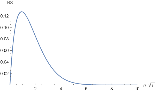
In this paper, we study the behaviour of the implied volatility for Inverse European options under general stochastic volatility pricing models. Specifically, we present analytical results for the asymptotic behaviour of the at-the-money level and skew of the implied volatility for a general stochastic volatility pricing model. Our main tool for proving these results is the anticipating Itô’s formula from the Malliavin calculus, see Appendix A for an introduction to this topic. We follow a similar approach as in Alòs [3] in order to derive formulas for the price and the implied volatility skew. This approach has been further developed in different setting. Recently, Muguruza et al. [4] apply this methodology for VIX options and in Alòs, Nualart, Pravosud [7] for Asian options. See also the references therein. The difference in the present paper among all the other papers using this method is that the Black-Scholes formula is different from the classical one. Instead, we need to work under the Black-Scholes formula for Inverse European calls under constant volatility obtained in [1], which turns out to be a non-monotonic function (see Figure 6) and thus its inverse is not defined uniquely, which makes the computations more challenging. We provide general sufficient conditions on a general stochastic volatility model in order to obtain the short time maturity asymptotic formulas for the at-the-money level and the skew of the implied volatility of Inverse options, and we apply it to two well-known models which are the SABR and fractional Bergomi models. This analysis allows us to obtain the same formulas for Quanto Inverse European options whose payoff is given by
where is a fixed exchange rate.
The paper is organized as follows. Section 2 is devoted to the statement of the problem and main results. Intermediary steps that allow us to prove the key theorems are presented in Section 3. The proof of the main results is given in Section 4. Finally, in Section 5 we present the numerical study in the case of the SABR and fractional Bergomi models.
2 Statement of the problem and main results
Consider the following model for the asset price on the time interval
| (1) |
where is fixed and , , and are three standard Brownian motions on defined on the same risk-neutral complete probability space . For the sake of simplicity (as in [4]) we assume that the interest rate is zero. We assume that and are independent and is the correlation coefficient between and . When the volatility is constant, this model is the regular Black-Scholes model.
We consider the following hypotheses on the volatility process.
Hypothesis 1.
The process is square integrable, adapted to the filtration generated by , a.s. positive and continuous, and satisfies that for all ,
for some positive constants and .
Hypothesis 2.
For all there exists and such that for all ,
Hypothesis 3.
For , (see the Appendix for the definition of this space).
Hypothesis 4.
There exists and for all there exist constants such that for all
| (2) |
and
where denotes the Malliavin derivative defined in the Appendix.
Let and denote the values of an Inverse European call and a Quanto Inverse European call options with fixed strike , respectively.
We have that
and
where is a fixed exchange rate. Notice that the difference between and is due to the currency in which the options are quoted. In our case is the crypto price of the option and is the dollar value of the option.
We denote by the Black-Scholes price of an Inverse European call option with time to maturity , log-underlying price , log-strike price and volatility . Then, it is well-known that (see Imeraj et al. [1]),
where is the cumulative distribution function of a standard normal random variable. Moreover, the Black-Scholes price of a Quanto Inverse European call is given by .
One can easily check that the Black-Scholes price satisfies the following PDE
| (3) |
Moreover, one can also check that the classical relationship between the Gamma, the Vega and the Delta holds, that is,
| (4) |
As in [3], we consider the log-forward price , which satisfies
Next, we observe that, as , the price of an Inverse call option can be written as
In particular, and . This implies that the implied volatility level and skew of Inverse and Quanto Inverse European call options are equal up to the factor . Hence, we will only state the main results of this paper for the Inverse options.
We define the implied volatility (IV) of an Inverse European call option as the quantity satisfying
We denote by , where , the corresponding at-the-money implied volatility (ATMIV) which, in the case of zero interest rates, takes the form .
The aim of this paper is to apply the Malliavin calculus techniques developed in Alòs [3] in order to obtain formulas for
under the general stochastic volatility model (1), where we have set for the sake of simplicity.
The main results of this paper are given in the following theorem.
Theorem 1.
Assume Hypotheses 1-4. Then,
| (5) |
Moreover,
| (6) | ||||
We observe that when prices and volatilities are uncorrelated then the short-time skew equals to zero. Observe also that if the term is of order , the limit of the right hand side of (6) will be if and it will converge to a constant when . When we need to multiply by in order to obtain a finite limit.
The results of Theorem 1 can be used in order to derive approximation formulas for the price of an Inverse and Quanto Inverse European call options. Notice that, as
by Taylor’s formula we can use the approximations
Of course, this approximation is only linear, and one would expect to obtain better results if one has a short maturity asymptotic formula for the curvature . The short-time maturity asymptotics for the at-the-level curvature of the implied volatility for European calls under general stochastic volatility models is computed in [5]. A Taylor expansion for short maturity asymptotics for Asian options when the underlying asset follows a local volatility model is obtained in [19]. In our setting, computing the curvature is more challenging and we leave it for further work.
3 Preliminary results
In this section we provide closed form decomposition formulas for the price and for the ATMIV skew of an Inverse call option under the stochastic volatility model (1).
We first need the following preliminary lemma. See Lemma 6.3.1 in [4] for the standard European call option case.
Lemma 1.
Assume Hypothesis 1. Then, for all there exist positive constants , and such that for all ,
| (7) | ||||
| (8) | ||||
| (9) |
where and
.
Proof.
Using Hypothesis 1, the fact that for all and the function is bounded, and that it is easy to see that the first term is bounded by .
For the second term, we use the fact that the function Erfc is bounded and that has bounded moments of all orders by Hypothesis 1. This completes the proof of (7).
We next prove (8). Straightforward differentiation gives
Then, due to Hypothesis 1, we get that
where .
Hence, using the fact that for all and the function is bounded and , we conclude that (8) holds true.
Finally, we have that
and the same argument as above allows us to complete the proof (9), and thus the proof of the Lemma. ∎
The main result of this section is the following theorem.
Theorem 2.
Assume Hypotheses 1-4. Then, the following relation holds
Proof.
We follow similarly as in Alòs [3]. Since the law of one price leads us to the conclusion that . Applying Theorem 4 in the Appendix to the function we get that
By adding and subtracting to the expression above we get that
Notice that the second term in the above expression is equal to zero due to formula (3). Finally, using equation (4) and taking expectation we complete the proof. Observe that by Lemma 1 and Hypotheses 1-4 all expectations are finite. In fact, Using Cauchy-Schwarz inequality, and Hypotheses 1 and (2), we get that
∎
We next derive an expression for the ATMIV skew of an Inverse European call option under the stochastic volatility model (1).
Proposition 1.
Proof.
This proof follows similarly as Theorem 4.2 in Alòs, León and Vives [6]. Since , the following equation holds
On the other hand, using Theorem 2, we get that
Combining both equations, we obtain that that the volatility skew is equal to
Finally, using the fact that
and Theorem 2 we conclude that
Straightforward differentiation gives us the following expression
| (11) |
By (5) . Moreover, by continuity, we have that . Thus, . Thus, since , we conclude that
which completes the proof. ∎
In order to compute the limit of the skew slope of the ATMIV, we need to identify leading order terms of the numerator in equation (10). This next decomposition formula will be crucial to attain this goal.
Proposition 2.
Assume Hypotheses 1-4. Then,
where and .
4 Proof of Theorem 1
4.1 Proof of (5) in Theorem 1: ATMIV level
This section is devoted to the proof of (5) in Theorem 1. The proof follows similar ideas as in Alòs and Shiraya [8].
4.1.1 The uncorrelated case
Notice that, if , Theorem 2 implies that . Then the implied volatility satisfies the following
where .
We observe that as , the two Brownian motions and are independent. Thus, and is a martingale wrt to the filtration . By the martingale representation theorem, there exists a square integrable and -adapted process such that
Clark-Ocone-Haussman formula (Theorem 3) gives us the following representation,
Then, a direct application of the classical Itô’s formula implies that
where and denote, respectively, the first and second derivatives of with respect to .
4.1.2 The correlated case
Using similar ideas as in the uncorrelated case we get that
where .
Then, a direct application of the Itôs formula gives us
By (7), we have that . Moreover, using Lemma 2 in Appendix B we have that for sufficiently small . Therefore, using Hypotheses 1 and 4 and Cauchy-Schwarz inequality, we get that
Thus, . Finally, using (12) we conclude the proof of (5) in the correlated case.
4.2 Proof of (6) in Theorem 1: ATM implied volatility skew
We start analysing the second term in (13). Using Hypotheses 1 and 4, (9) and Cauchy-Schwarz inequality, we get that
Hypothesis 1 implies that
Next, Hypotheses 1 and 4 together with Cauchy-Schwarz inequality yield to
Then, using the computations above together with (8), we get that
5 Numerical analysis
In this section we justify Theorem 1 with numerical simulations. Notice that the SABR and fractional Bergomi models do not satisfy Hypothesis 1. However, a truncation argument justifies the application of Theorem 1 in these cases. Since the truncation argument is exactly the same as in Alòs, Nualart, Pravosud [7] and we safely skip it.
5.1 The SABR model
In this section we consider the SABR stochastic volatility model with skewness parameter equal to 1, which is the most common case from a practical point of view. This corresponds to equation (1), where denotes the forward price of the underlying asset and
where is the volatility of volatility.
For , we have that and . Therefore, applying Theorem 1 we conclude that
We next proceed with some numerical simulations using the following parameters
In order to get estimates of the Inverse European call option we use antithetic variates. The estimate of the price is calculated as follows
| (14) | ||||
where and the sub-index denotes the value of a call option computed on the antithetic trajectory of a Monte Carlo path.
In order to retrieve the implied volatility we use Brent’s method. For the estimation of the skew, we use the following expression which allows us to avoid a finite difference approximation of the first order derivative.
| (15) | ||||
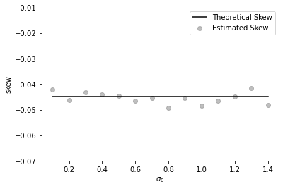
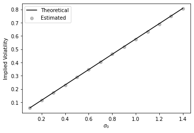
In Figure 1 and 2 we present the results of a Monte Carlo simulation which aims to estimate numerically the skew and the level of the at-the-money implied volatility of the Inverse European call option under the SABR model. We conclude that numerical results fit the theoretical ones.
 |
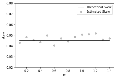 |
| (a) =-0.3 | (b) =0.3 |
5.2 The fractional Bergomi model
Moreover, for , we have
which gives
and for
The parameters used for the Monte Carlo simulation are the following
In order to get estimates of the price of the Inverse European call option under the fractional Bergomi model we use antithetic variates presented in equations (14). We use equation (15) for the estimation of the skew.
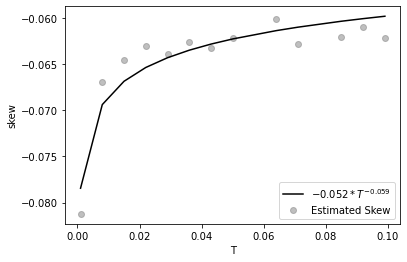
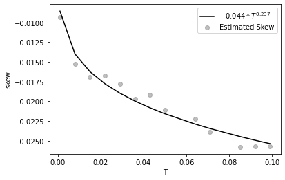
On Figure 3 we present the ATM implied volatility skew as a function of maturity of the Inverse European call option for two different values of , where we observe the blow up to for the case .
 |
 |
| (a) H=0.4, | (b) H=0.7, |
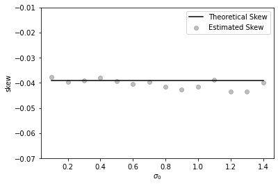
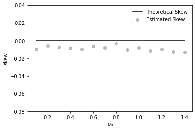
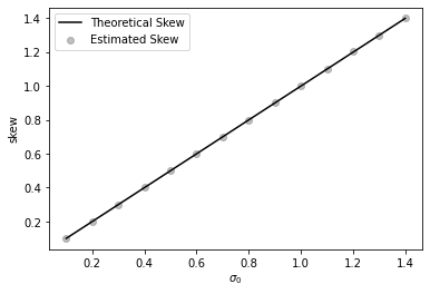
Due to the blow up of the at-the-money implied volatility skew of the Inverse European call option when we also plot the quantities for and for on Figure 4. And in Figure 5 we present the estimates of ATM IV level. In general, we conclude that theoretical results are in line with values provided by Theorem 1.
 |
 |
| (a) H=0.4 | (b) H=0.7 |
 |
 |
| (a) H=0.4 | (b) H=0.7 |
Appendix A A primer on Malliavin Calculus
We introduce the elementary notions of the Malliavin calculus used in this paper (see Nualart and Nualart [18]). Let us consider a standard Brownian motion defined on a complete probability space and the corresponding filtration generated by . Let be the set of random variables of the form
with , denotes the Wiener integral of the function , for , and (i.e., and all its partial derivatives are bounded). Then the Malliavin derivative of , , is defined as the stochastic process given by
This operator is closable from to , for all , and we denote by the closure of with respect to the norm
We also consider the iterated derivatives for all integers whose domains will be denoted by , for all . We will use the notation . One of the main results in Malliavin calculus is the Clark-Ocone-Haussman formula:
Theorem 3.
Let . Then
The following theorem is an extension of classical Ito’s lemma for the case of non-anticipating processes, see Alòs [3] for details.
Theorem 4 (Anticipating Itô’s Formula).
Consider a process of the form
where is an -measurable random variable and and are -adapted processes in .
Consider also a process , for some . Let be a function such that there exists a positive constant such that, for all , and its derivatives evaluated in are bounded by . Then it follows that for all ,
where .
Appendix B The ATM Inverse call option price
Recall that ATM value of an Inverse call option is given by
We plot this function in Figure 6 as a function of and we observe that the function is not monotone in all its domain so the inverse with respect to will not be uniquely defined. However, since we only need the study of the function for small values of , then in that case the function is monotone increasing and the inverse will be well defined in a small positive interval around .
Lemma 2.
Under Hypothesis 1, for all sufficiently small there exists a positive constant such that for all ,
where .
Proof.
We have that
Recall form (11) that
where . Therefore, we conclude that
Notice that and for sufficiently small, the function is non-negative and monotonically decreasing on the interval . Since it is continuous it is lower bounded by a positive constant on that interval. On the other hand, is also small for sufficiently small , so the inverse is well-defined in this case. This completes the desired proof. ∎
Lemma 3.
Under Hypothesis 1, for all sufficiently small there exists a positive constant such that for all ,
where .
Proof.
We have that
Therefore,
where . Notice that and for sufficiently small, the function is non-negative and monotonically increasing on the interval . Since it is continuous it is upper bounded by a positive constant on that interval. On the other hand, is also small for sufficiently small , so the inverse is well-defined in this case. This completes the desired proof. ∎
References
- [1] Carol Alexander, Ding Chen, and Arben Imeraj. Inverse and Quanto Inverse Options in a Black-Scholes World. Mathematical Finance, 33(4):1005–1043, 2023.
- [2] Carol Alexander and Arben Imeraj. Delta Hedging Bitcoin Options with a Smile. Quantitative Finance, 23(5):799–817, 2023.
- [3] Elisa Alòs. A generalization of the Hull and White formula with applications to option pricing approximation. Finance and Stochastics, 10(3):353–365, 2006.
- [4] Elisa Alòs, David García-Lorite, and Aitor Muguruza Gonzalez. On Smile Properties of Volatility Derivatives: Understanding the VIX Skew. SIAM Journal on Financial Mathematics, 13(1):32–69, 2022.
- [5] Elisa Alòs and Jorge A. León. On the curvature of the smile in stochastic volatility models. SIAM Journal on Financial Mathematics, 8:373–399, 2017.
- [6] Elisa Alòs, Jorge A. León, and Josep Vives. On the short-time behavior of the implied volatility for jump-diffusion models with stochastic volatility. Finance and Stochastics, 11(4):571–589, 2007.
- [7] Elisa Alòs, Eulalia Nualart, and Makar Pravosud. On the implied volatility of Asian options under stochastic volatility models. http://arxiv.org/abs/2208.01353, 2023.
- [8] Elisa Alòs and Kenichiro Shiraya. Estimating the Hurst parameter from short term volatility swaps: a Malliavin calculus approach. Finance and Stochastics, 23(2):423–447, 2019.
- [9] Saifedean Ammous. Can cryptocurrencies fulfil the functions of money? The Quarterly Review of Economics and Finance, 70:38–51, 2018.
- [10] Thomas Ankenbrand and Denis Bieri. Assessment of cryptocurrencies as an asset class by their characteristics. Investment Management and Financial Innovations, 15(3):169–181, 2018.
- [11] Olyga S. Bolotaeva, Amalia A. Stepanova, and Sofia S. Alekseeva. The Legal Nature of Cryptocurrency. IOP Conference Series: Earth and Environmental Science, 272(3):032166, 2019.
- [12] Mark B. Garman and Steven W. Kohlhagen. Foreign currency option values. Journal of International Money and Finance, 2(3):231–237, 1983.
- [13] Stéphane Goutte, Khaled Guesmi, and Samir Saadi. Cryptofinance. WORLD SCIENTIFIC, 2021.
- [14] Marc Gronwald. Is Bitcoin a Commodity? On price jumps, demand shocks, and certainty of supply. Journal of International Money and Finance, 97:86–92, 2019.
- [15] Peter K. Hazlett and William J. Luther. Is bitcoin money? And what that means. The Quarterly Review of Economics and Finance, 77:144–149, 2020.
- [16] Ai Jun Hou, Weining Wang, Cathy Y H Chen, and Wolfgang Karl Härdle. Pricing Cryptocurrency Options. Journal of Financial Econometrics, 18(2):250–279, 2020.
- [17] Jovanka Lili Matic, Natalie Packham, and Wolfgang Karl Härdle. Hedging cryptocurrency options. Review of Derivatives Research, 26(1):91–133, 2023.
- [18] David Nualart and Eulalia Nualart. Introduction to Malliavin Calculus. Cambridge University Press, 2018.
- [19] Dan Pirjol and Lingjiong Zhu. Short maturity Asian options in local volatility models. SIAM Journal on Financial Mathematics, 7:947–992, 2016.
- [20] Tak Kuen Siu and Robert J. Elliott. Bitcoin option pricing with a SETAR-GARCH model. The European Journal of Finance, 27(6):564–595, 2021.