Diff-PCR: Diffusion-Based Correspondence Searching in Doubly Stochastic Matrix Space for Point Cloud Registration

Abstract

Efficiently finding optimal correspondences between point clouds is crucial for solving both rigid and non-rigid point cloud registration problems. Existing methods often rely on geometric or semantic feature embedding to establish correspondences and estimate transformations or flow fields. Recently, state-of-the-art methods have employed RAFT-like iterative updates to refine the solution. However, these methods have certain limitations. Firstly, their iterative refinement design lacks transparency, and their iterative updates follow a fixed path during the refinement process, which can lead to suboptimal results. Secondly, these methods overlook the importance of refining or optimizing correspondences (or matching matrices) as a precursor to solving transformations or flow fields. They typically compute candidate correspondences based on distances in the point feature space. However, they only project the candidate matching matrix into some matrix space once with Sinkhorn or dual softmax operations to obtain final correspondences. This one-shot projected matching matrix may be far from the globally optimal one, and these approaches do not consider the distribution of the target matching matrix. In this paper, we propose a novel approach that exploits the Denoising Diffusion Model to predict a searching gradient for the optimal matching matrix within the Doubly Stochastic Matrix Space. Our method incorporates the diffusion model to learn a denoising gradient direction. During the reverse denoising process, our method iteratively searches for better solutions along this denoising gradient, which points towards the maximum likelihood direction of the target matching matrix. To improve efficiency, we employ a lightweight design for our denoising module and utilize the sampling strategy in the Denoising Diffusion Implicit Model (DDIM[27]). Experimental evaluations on the 3DMatch/3DLoMatch and 4DMatch/4DLoMatch datasets demonstrate the effectiveness of our newly designed framework.

Figure 1: The reverse sampling process for matching matrix on the doubly stochastic matrix manifolds. Zoom in for details.

I Introduction

Matching pairwise point clouds from different scans is a fundamental task in various computer vision applications, including point cloud registration[1], scene flow estimation[2], and localization[3]. These applications often involve scenes with rigid transformations or non-rigid deformations, which require accurate correspondences between points.

Learning-based methods[4, 5, 6, 7, 8] have made significant advancements in point cloud registration, with the use of backbones like KPConv[9] to obtain subsampled super points and their associated features. These methods typically calculate an initial matching matrix between super points in the feature space. Outlier rejection techniques[10, 11] can be employed to improve inlier correspondences using specially designed networks[12, 13, 14] or priors[15]. However, these methods usually use a one-shot prediction strategy for correspondences, leaving room for further improvement.

Some recent works[16, 5, 2, 17] employ RAFT-like[18] iterative refinement in their frameworks, resulting in significant performance improvements. However, there is no explicit theoretical explanation for why these methods typically only iterate a few times to achieve the best result. The term ’best’ means if they conduct more iterative times, the performance decreases again! Some approaches[8, 19, 20] realize that utilizing traditional optimization methods can provide a more explicit explanation of the solution search process. However, due to the complex domain of solutions, the iterative optimization process may become trapped in suboptimal positions or be driven by non-feasible gradient directions. These methods do not learn the searching gradient through a feature backbone that is highly related to the dataset prior.

In this study, inspired by the reverse sampling process in DDPM[21], conditional gradient in Frank-Wolfe algorithm[22], and score-based MCMC approaches (Langevin MCMC[23] and HMC[24]), we propose a robust framework for optimizing the matching matrix in the space of doubly stochastic matrices[25]. We argue that the optimization of solutions should occur in the feasible solution space, and the searching gradient can be learned by the network instead of relying implicitly on the RAFT-like[18, 26] iterations. By adopting this searching gradient, the iterative optimization process can aim for the globally optimal target matching matrix while being less sensitive to the starting point.

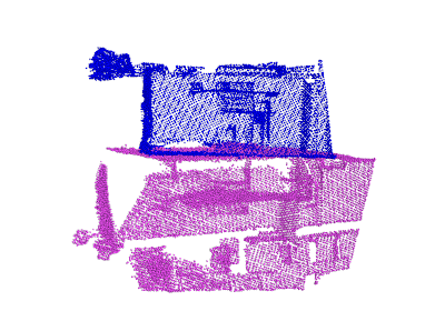
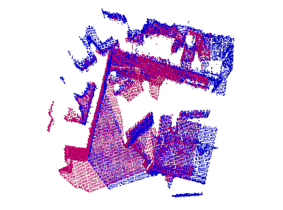
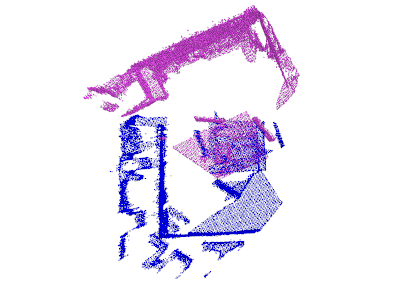
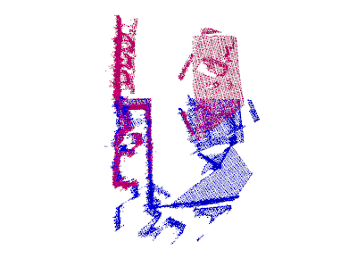
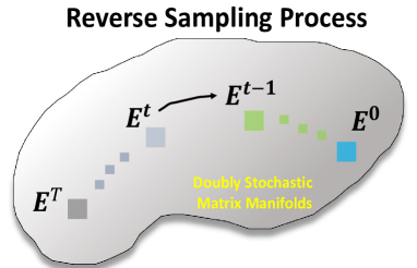
Our framework incorporates the Gaussian reverse sampling technique, adapted from DDPM [21], to facilitate the iterative optimization process starting from the initial solution of the matching matrix. We assume that the solution domain of the matching matrix is the doubly stochastic matrix space, as it represents a continuous relaxation of the discrete matching matrix space. Thus, we can apply the continuous Gaussian denoising step in this continuous doubly stochastic matrix space. During the sampling process, we employ the sinkhorn algorithm to enforce constraints on the intermediate solution within the doubly stochastic matrix space (see in Fig.(1)). Unlike deterministic iterative optimization methods mentioned earlier, our approach introduces Gaussian noise during the sampling step. This effectively prevents the algorithm from getting trapped in local optima, enabling a more extensive exploration of the solution domain space. Our iterative searching gradient is more robust, offering more diversity and allowing for more iterative steps.

To enhance efficiency, we apply the DDIM[27] schedule to accelerate the sampling speed. Our model consists of one KPConv[9] feature backbone and one denoising module. We empirically demonstrate that the simplistic noise model design does not negatively impact performance.

Our contributions are summarized as follows:

• To the best of our knowledge, we are the first to utilize the diffusion model in the doubly stochastic matrix space for iteratively searching optimal matching matrix solutions using the reverse sampling process. This matching matrix diffusion model can be integrated as a module in any other 2D-2D, 2D-3D, and 3D-3D registration problems.

• The lightweight design of our reverse denoising module results in faster convergence during the iterative optimization process. Moreover, our framework is capable of effectively utilizing reverse denoising sampling in a noise-to-target fashion or starting from a highly reliable initial solution generated by the point features of the backbone.

• We conducted comprehensive experiments on the 3DMatch/4DMatch datasets to validate the efficacy of our methods in predicting the matching matrix for scenes involving both rigid transformations and non-rigid deformations. These experiments involved rigorous evaluation and comparison with state-of-the-art approaches, demonstrating the competitive performance and effectiveness of our proposed framework.

II Related work

II-A Point cloud Regsitration

Recently, significant improvements have been made in feature learning-based point cloud registration methods. Many of them[28, 29, 30, 4, 31, 32, 16] rely on the KPConv[9] backbone to downsample super points and generate associate features with larger receptive fields. To further improve performance, these methods incorporate prior knowledge and design learnable outlier rejection modules. For example, they[31] inject the local PPF[33] features into the transformer to enhance the rotation invariance. PEAL[16] utilizes a pre-trained registration model to give overlap information as an overlap prior and employ simple attention across the overlap and non-overlap region. Subsequently, a GeoTR[4] network is exploited to conduct the iterative updates.

In addition, another category of registration methods focuses on outlier rejection of candidate correspondences. For example, PointDSC[10] exploits a max clique algorithm in the local patch to cluster the inlier correspondences. SC2-PCR[11] constructs a second-order consistency graph for candidate correspondences and proves theoretically its robustness. Based on the second-order consistency graph from SC2-PCR[11], MAC[15] develops a variant of the max clique algorithms to provide more reliable candidate inlier correspondences. Furthermore, methods like PEAL[16], and DiffusionPCR[34] employ a iterative refinement strategy to improve the given overlap prior information obtained from a pre-trained point cloud registration method.

II-B Diffusion Models for Registration

Recently, the diffusion model[21, 35, 27] has made greate development in many fields, including object detection[36], image generation[37], text-to-image translation[38]. These developments have been achieved through a generative Markov Chain process based on the Langevin MCMC[23] or a reversed diffusion process[27]. Recognizing the power of the diffusion model to iteratively approximate target data distributions from white noise using hierarchical variational decoders, researchers have started applying it to point cloud registration and 6D pose estimation problems.

The pioneer work[39] that applied the diffusion model in the SE(3) space was accomplished by utilizing NCSN[35] to learn a denoising score matching function. This function was then used for reverse sampling with Langevin MCMC in SE(3) space to evaluate 6DoF grasp pose generation. Additionally, [40] implemented DDPM[21] in the SE(3) space for 6D pose estimation by employing a surrogate point cloud registration baseline model. Similarly, GeoTR[4] was employed as a denoising module in[34], gradually denoising the overlap prior given by the pre-trained model, following a similar approach to PEAL[16]. In contrast to these methods, our approach conducts the diffusion process in the doubly stochastic matrices manifolds, which applies to both rigid and deformable registration tasks. By considering the constraints of the matching matrix in the doubly stochastic matrices manifolds, our method addresses ambiguities (such as symmetry or global repeatability) in registration, which were not explicitly addressed in previous works.

III The proposed Approach

III-A Problem Formulation

Given source point clouds $P\in\mathbb{R}^{N{\times}3}$ and target points $Q\in\mathbb{R}^{M{\times}3}$, the registration task is to find top-K correspondences $K$ from matching matrix $E$ and to conduct warping between them to align $P$ and $Q$. For the rigid case, the warping operation $W$ is parameterized by transformation $T\in$ SE(3). In the deformation case, the warping operation can be treated as flow fields from source $P$ to target $Q$ per point. Give ground truth warping operation $W_{gt}$, and for every correspondence ($p_{i}\in P$ and $q_{j}\in Q$), the constraint $||W_{gt}(p_{i})-q_{j}||_{2}<\sigma$ should be satisfied, where $\sigma$ is a threshold, and $||\cdot||_{2}$ is the Euclidean norm.

III-B Preliminaries

Revisiting Diffusion Model. Diffusion models[41, 21, 27, 35, 42] are a likelihood-based Markovian Hierarchical Variational Autoencoder (HVAE)[43]. The joint distribution and posterior of a variational diffusion model are defined as follows:

$$p(\mathit{x_{0}},\mathit{x}_{1:T})=p(x_{T})p_{\theta}(x_{0}|x_{1})\prod_{t=2}^{T}p_{\theta}(x_{t-1}|x_{t})$$ (1)

$$q_{\phi}(x_{1:T}|x_{0})=q_{\phi}(x_{1}|x_{0})\prod_{t=2}^{T}q_{\phi}(x_{t}|x_{t-1}).$$ (2)

Due to the assumption of Gaussian transition kernel $q(x_{t}|x_{t-1})$ utilized in the DDPM[21] according to a variance schedule $\beta_{1},...,\beta_{T}$:

$$q(x_{t}|x_{t-1})=\mathcal{N}(x_{t};\sqrt{\alpha_{t}}x_{t-1},(1-\alpha_{t})\textbf{I}),$$ (3)

the diffused $x_{t}$ at an arbitrary timestep t has a closed form:

$$q(x_{t}|x_{0})=N(x_{t};\sqrt{\bar{\alpha}}x_{0},(1-\bar{\alpha})\textbf{I}))$$ (4)

where $\alpha_{t}=1-\beta_{t}$ and $\bar{\alpha}=\prod_{s=1}^{t}\alpha_{s}$.

For an arbitrary sample $x_{t}\sim q(x_{t}|x_{0})$, we can rewrite is as:

$$\begin{split}x_{t}&=\sqrt{\bar{\alpha}_{t}}x_{0}+\sqrt{1-\bar{\alpha_{t}}}\epsilon_{0}\\ &\sim N(x_{t};\sqrt{\bar{\alpha}_{t}}x_{0},(1-\bar{\alpha_{t}})\textbf{I})\end{split}$$ (5)

Based on Eqn.3, Eqn.4, and Eqn.5 and utilize the Bayes rule, the denoising step can be derived as:

$$\begin{split}&q(x_{t-1}|x_{t},x_{0})=\frac{q(x_{t}|x_{t-1},x_{0})q(x_{t-1}|x_{0})}{q(x_{t}|x_{0})}\\ &\propto N(x_{t-1};\underbrace{\frac{\sqrt{\alpha_{t}}(1-\bar{\alpha}_{t-1})x_{t}+\sqrt{\bar{\alpha}_{t-1}}(1-\alpha_{t})x_{0}}{1-\bar{\alpha}_{t}}}_{\mu_{q}(x_{t},x_{0})},\\ &\underbrace{\frac{(1-\alpha_{t})(1-\bar{\alpha}_{t-1})}{1-\bar{\alpha}_{t}}\textbf{I}}_{\Sigma_{q}(t)}).\end{split}$$ (6)

Based on equation Eqn.2 and rewritten form of transition kernel $q(x_{t}|x_{t-1})=q(x_{t}|x_{t-1},x_{0})$ (due to Markov property), we can derive the ELBO:

$$\begin{aligned} &logp(x_{0})\geq-L_{vb}=\\ &\underbrace{\mathbb{E}_{q(x_{1}|x_{0})}[logp_{\theta}(x_{0}|x_{1})]}_{reconstruction\ term}-\underbrace{D_{KL}(q(x_{T}|x_{0}||p(x_{T})))}_{prior\ matching\ term}\\ &-{\sum\limits_{T=2}^{T}}\underbrace{\mathbb{E}_{q(x_{t}|x_{0})}[D_{KL}(q(x_{t-1}|q_{x_{t}},x_{0}))||p_{\theta}(x_{t-1}|x_{t})]}_{denoising\ matching\ term}\end{aligned}$$ (7)

By some derivations[43], the optimization of denoising matching term (in Eqn.7) boils down to learning a network $g_{\theta}(x_{t})$ to predict the ground truth $x_{0}$ (i.e., in $\mu_{q}(x_{t},x_{0})$) from an arbitrarily diffused version $x_{t}$:

$$\begin{split}&\underset{\theta}{\arg\min}\,D_{KL}(q(x_{t-1}|x_{t},x_{0})||p_{\theta}(x_{t-1}|x_{t}))\\ =&\underset{\theta}{\arg\min}\,\frac{1}{2\sigma_{q}^{2}(t)}\frac{\bar{\alpha}_{t-1}(1-\alpha_{t})^{2}}{(1-\bar{\alpha}_{t})^{2}}\left[||g_{\theta}(x_{t})-x_{0}||\right]\end{split}$$ (8)

where ${\sigma_{q}^{2}}(t)=\frac{(1-\alpha_{t})(1-\bar{\alpha}_{t-1})}{1-\bar{\alpha}_{t}}$.

After training the $g_{\theta}(\cdot)$, we can use this reverse transition step $p_{\theta}(x_{t-1}|x_{t}))$ to sample the target from any given initialization $x_{T}$.

Revisiting Doubly Stochastic Matrix. We can represent the point clouds $P$ and $Q$ as two graphs, denoted as $\mathcal{G}_{1}=\left\{P,E^{P}\right\}$ and $\mathcal{G}_{2}=\left\{Q,E^{Q}\right\}$, where $E^{P}$ and $E^{Q}$ are respective edge sets. The matching matrix between these two graphs is a one-to-one mapping $E\in\{0,1\}^{N{\times}M}$. In cases where $N\neq M(e.g.,N>M)$, we can introduce $N-M$ dummy points in $Q$ to make a square matching matrix, also known as a permutation matrix:

$$\mathcal{D}=\left\{A:A1_{N}=1_{N},A^{T}1_{N}=1_{N},A\geq 0\right\}.$$ (9)

To transform an intermediate non-negative real matrix into a ”doubly stochastic” matrix, which has uniform row sum M and column sum N[25], we can employ sinkhorn iterations[44]. Since the correspondence between two scans of point clouds must satisfy the one-to-one constraints, many works project the correspondences via sinkhorn[44] into this doubly stochastic matrix space.

However, in real-world scenarios, the two scans of point clouds only partially overlap. Most parts of the matching matrix have values of 0, while the truly corresponding slots have a value of 1. As a result, many previous works[4, 5] adopt the top-K confident matches from the relaxed ”doubly stochastic” matching matrix (where the uniform row sum is $\leq M$ or column sum is $\leq N$) as candidate correspondences. Hence, these approaches inspire us to model the partial matching matrix within a relaxed ”doubly stochastic” matching matrix space $\mathcal{M}$ and learn a search gradient to find the most reliable solution (the 0-valued elements are supposed to be close to a tiny value like $1e^{-5}$) with its top-k slots close to the ground truth correspondences. In this case, the backward optimization step can optimize the relative order of potential matching scores rather than their absolute magnitude by the supervision.

The images or point clouds obtained from sensors undergo scale transformation and perspective changes. The data of scenes exhibit symmetry, globally repeating, as well as phenomena like noise or non-rigid deformation. Matrix space can effectively represent these phenomena and has higher dimensions than low dimensions space,(e.g., SE(3) and $\mathbb{R}^{3N}/\mathbb{R}^{2N}$). Therefore, searching directly in the matching matrix space theoretically enables us to find better solutions. In the registration tasks, the many-to-one relationship between the matching matrix space and the warping operation space serves as motivation for us to propose searching in the matching matrix space:

Hypothesis 1.

If there is a network that can accurately predict the matching degree between $p_{i}$ and $q_{j}$ with its score $E_{ij}$, and if there is an efficient optimization algorithm capable of searching in the matrix space, then under these conditions, searching for the optimal solution in the match matrix space may yield superior results compared to direct search in low-dimensional spaces(e.g., SE(3) and $\mathbb{R}^{3N}/\mathbb{R}^{2N}$)

For instance, we can give an informal formulation of the rigid scene:

$$\underset{E\in\mathcal{M}}{\min}\sum\limits_{i=1}^{N}\sum\limits_{j=1}^{M}E_{ij}*||W_{E}(p_{i})-q_{j}||_{2}$$

$$\leq\mathop{\min}\limits_{W\in SE(3)}\sum\limits_{i=1}^{N}\sum\limits_{j=1}^{M}\hat{E}_{ij}*||W(p_{i})-q_{j}||_{2}$$ (10)

where $W_{E}$ is a warping that generated based on $E$ and $\hat{E}$ is a fixed matching matrix pre-computed.

Figure 2: Overview of our matching matrix diffusion model. $\bigoplus$ mean 3D point coordinates and position encoding are both utilized as input. $\bigotimes$ means only 3D point utilized. The input points $\hat{P},\hat{Q}$ along with their corresponding point features $F^{\hat{P}},F^{\hat{Q}}$ remain fixed throughout the entire reverse sampling process after being output from the KPConv backbone. These inputs undergo transformation through the warping operation and denoising transformer at each denoising step. The forward diffusion process is modeled by the Gaussian transition kernel $q(E^{t}|E^{t-1})$ which has a closed form $q(E^{t}|E^{0})$. The denoising model $g_{\theta}(E^{t})$ learns a reverse denoising gradient that points to the target solution $E^{0}$. During inference in the reverse sampling process, we utilize the predicted $\hat{E}_{0}$ and Eqn. (5,15) to sampling $E^{t-1}$.

III-C Framework Overview

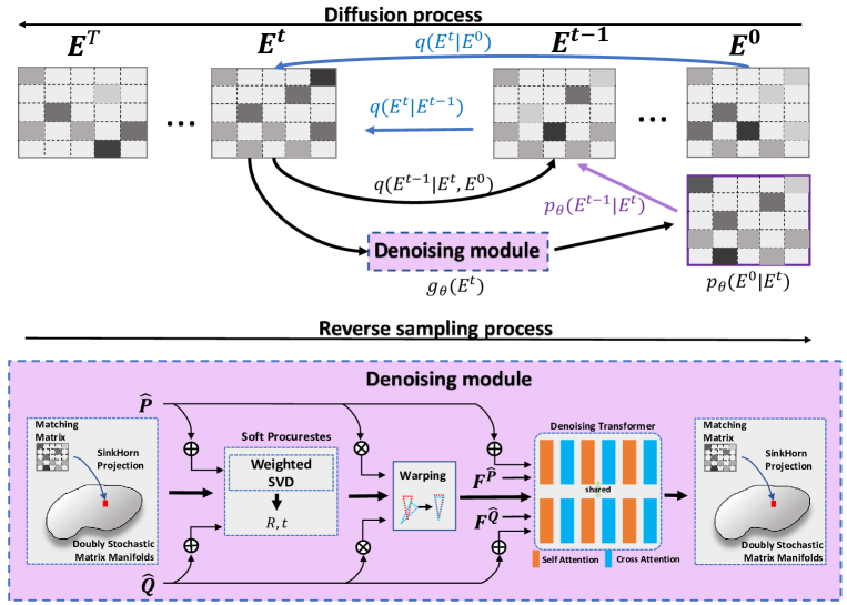
Our framework consists of a KPConv[9] feature backbone and one diffusion model[21]. The backbone takes source point clouds $P$ and target $Q$ as input and performs three downsamplings and two upsamplings to obtain the downsampled super points $\hat{P}$ and $\hat{Q}$, along with their associated features associate features $F^{\hat{P}}\in\mathbb{R}^{N{\times}d}$ and $F^{\hat{Q}}\in\mathbb{R}^{M{\times}d}$. The initilized matching matrix $E^{T}$ is sampled from white noise or computed by the inner product of $F^{\hat{P}}$ and $F^{\hat{Q}}$. We then employ the denoising module $g_{\theta}$ (III-E) to reverse sample the target matching matrix $E^{0}$.

The denoising module $g_{\theta}$ mainly comprises four different key components:

• Sinkhorn Projection[44], $\mathbf{f_{sinkhorn}(\cdot)}$, is responsible for projecting the input matrix into the Doubly Stochastic Matrix space (see III-E1).

• Weighted SVD[45] $\mathbf{soft\_procrustes(\cdot,\cdot,\cdot)}$ is used to compute the transformation R and t (see III-E2).

• Denoising transformer network, $f_{\theta}(\cdot,\cdot,\cdot,\cdot,\cdot,\cdot)$, is responsible for calculating the denoised point features during the denoising step (see III-E4).

• The $\mathbf{matching\_logits(\cdot,\cdot,\cdot,\cdot)}$ function is utilized for computing the matching matrix between $\hat{P}$ and $\hat{Q}$ (see III-E5).

III-D Diffusion Model in Doubly Stochastic Matrix space

In this section, we present the construction of a diffusion model for generating the matching matrix of two scans. We denote the matching matrix $E\in\{0,1\}^{N{\times}M}$, and we assume $E$ is defined in a so-called nonsquare ”doubly stochastic” matrix space $\mathcal{M}$.

Diffusion Process. As mentioned in DDPM[21], the forward diffusion process is a Markovian process, denoted as $q(E^{1:T}|E^{0})=\prod_{t=1}^{T}q(E^{t}|E^{t-1})$, which generates a sequence of increasing noisier latent variables $E^{t}$ from the target $E^{0}$ to the white noise $q(E^{T})\sim N(0,\textbf{I})$. According to Eqn.4, the sampling matching matrix $E^{t}$ at arbitrary timestep t has a closed form:

$$q(E^{t}|E^{0})=N(E^{t};\sqrt{\bar{\alpha}}E^{0},(1-\bar{\alpha})\textbf{I})).$$ (11)

where the adding noise for each matrix element is sampled i.i.d. However, this sampled $E^{t}\sim q(E^{t}|E^{0})$ is a continuous matrix in $R^{N\times M}$, which is not within the feasible solution space of matching matrices (i.e., Doubly Stochastic Matrix manifolds). To address this, we apply the following projection to confine the sampled $E^{t}$ to $\mathcal{M}$:

$$\tilde{E}^{t}=sigmoid(E^{t}),\ \tilde{E}^{t}=\mathbf{f_{sinkhorn}}(\tilde{E}^{t})$$ (12)

where the $\mathbf{f_{sinkhorn}}$ operation is absorbed into the denoising module $g_{\theta}(\cdot)$.

Reverse denoising sampling. To generate the target matching matrix $E^{0}$, we need to learn the reverse transition kernel $q(E^{t-1}|E^{t},E^{0})$. Based on the Markov property, $q(E^{t-1}|E^{t},E^{0})$ can be rewritten as:

$$q(E^{t-1}|E^{t},E^{0})=\frac{q(E^{t}|E^{t-1},E^{0})q(E^{t-1}|E^{0})}{q(E^{t}|E^{0})}$$ (13)

and it is defined only depend on $\alpha_{t}$,$\bar{\alpha}_{t}$,and $E^{0}$ (see Eqn.6).

Then, we utilize the denoising module $g_{\theta}(\cdot)$ to predict the target $\hat{E}^{0}\in\mathcal{M}$. We exploit the continuous denoising step in DDIM[27] to compute the denoising gradient in the $\mathbb{R}^{N\times M}$ space.

$$\epsilon_{t}=\frac{\hat{E}_{0}}{\sqrt{1-\bar{\alpha}_{t}}}-\frac{\sqrt{\bar{\alpha}_{t}}}{\sqrt{1-\bar{\alpha}_{t}}}E^{t},$$ (14)

$$\hat{E}^{t-1}=\sqrt{\alpha_{t-1}}+\sqrt{1-\alpha_{t-1}-\sigma^{2}_{t}}\epsilon_{t}+\sigma_{t}z_{t},$$ (15)

where $\sigma_{t}=\sqrt{(1-\alpha_{t-1})/(1-\alpha_{t})}\sqrt{1-\alpha_{t}/\alpha_{t-1}}$ and $z_{t}\sim N(0,\textbf{I})$. The details of $g_{\theta}(E^{t})$ can be found in III-E.

Remarks. We empirically observed that not confining the matrix $E^{t}$ within $\mathcal{M}$ led to better performance. The reason behind this improvement could be that allowing $E^{t}$ to take continuous values in $\mathbb{R}^{N\times M}$ enables the computation of continuous gradients, which may provide a more extensive exploration of possible directions and ultimately point towards a more optimal solution.

Optimization loss. Inspired by [46] and Eqn.8, we replace the ”denoising matching term” in ELBO (Eqn.7) by a simplified version:

$$L_{simple}=-\mathbb{E}_{q(\hat{E}^{0})}\left[\sum\limits_{t-1}^{T}\left(\frac{T-t+1}{T}\right)\mathbb{E}_{q(E^{t}|\hat{E}^{0})}logp_{\theta}(\hat{E}^{0}|E^{t})\right]$$ (16)

where the reweighting term $\frac{T-t+1}{T}$ means that the loss at time steps close to T are weighted less than earlier steps. We give a brief derivation about this replacement $\mathbb{E}_{q(x_{t}|x_{0})}[D_{KL}(q(x_{t-1}|q_{x_{t}},x_{0}))||p_{\theta}(x_{t-1}|x_{t})]\rightarrow\mathbb{E}_{q(E^{t}|\hat{E}^{0})}logp_{\theta}(\hat{E}^{0}|E^{t})$:

$$\begin{aligned} &logp(E^{0})\geq\mathbb{E}_{E^{1:T}\sim q(E^{1:T}|E^{0})}\left[log\left(\frac{p_{\theta}(E^{0:T})}{q(E^{1:T}|E^{0})}\right)\right]\\ &=\mathbb{E}_{q}\left[log\left(\frac{p_{\theta}(E^{0:T})}{q(E^{1:T}|E^{0})}\right)\right]\\ &=\mathbb{E}_{q}\left[logp_{\theta}(E^{T})+log(\frac{p_{\theta}(E^{0}|E^{1})}{q(E^{1}|E^{0})})+\sum\limits_{t=2}^{T}log(\frac{{\color[rgb]{1,0,0}\definecolor[named]{pgfstrokecolor}{rgb}{1,0,0}p_{\theta}(E^{t-1}|E^{t})}}{{\color[rgb]{0,0,1}\definecolor[named]{pgfstrokecolor}{rgb}{0,0,1}q(E^{t}|E^{t-1})}})\right]\\ &=\mathbb{E}_{q}\left[logp_{\theta}(E^{T})+log(\frac{p_{\theta}(E^{0}|E^{1})}{q(E^{1}|E^{0})})\right]\\ &+\mathbb{E}_{q}\left[\sum\limits_{t=2}^{T}log\left({\color[rgb]{0,0,1}\definecolor[named]{pgfstrokecolor}{rgb}{0,0,1}\frac{q(E^{t-1}|E^{0})}{q(E^{t}|E^{0})}}\cdot\frac{{\color[rgb]{1,0,0}\definecolor[named]{pgfstrokecolor}{rgb}{1,0,0}q(E^{t-1}|E^{t},E^{0})p_{\theta}(E^{0}|E^{t})}}{{\color[rgb]{0,0,1}\definecolor[named]{pgfstrokecolor}{rgb}{0,0,1}q(E^{t-1}|E^{t},E^{0})}}\right)\right]\\ &=\mathbb{E}_{q}\left[S_{\theta}(E^{T},E^{1},E^{0})+\sum\limits_{t=2}^{T}log(p_{\theta}(E^{0}|E^{t}))\right]\end{aligned}$$

where $S_{\theta}(E^{T},E^{1},E^{0})=log\left(\frac{p_{\theta}(E^{T})}{q(E^{T}|E^{0})}\right)+log(p_{\theta}(E^{0}|E^{1}))$ and the blue equality is from Eqn.13. Since we employ the denoising module $g_{\theta}(\cdot)$ to predict the target $E^{0}$, we can reparameterize the $p_{\theta}(E^{t-1}|E^{t})$ as:

$$p_{\theta}(E^{t-1}|E^{t})\propto q(E^{t-1}|E^{t},E^{0})p_{\theta}(E^{0}|E^{t}).$$ (17)

Sampling strategy. We deploy two sampling strategies in the reverse sampling process: a) starting from white noise (i.e., $E^{T}\sim N(0,\textbf{I})$), b) starting from a reliable initialization. To accelerate, we utilize a sub-sequence $\tau$ of $[1,...,T]$ which $\sigma$ is indexed:

$$\sigma_{\tau_{i}}(\eta)=\eta\sqrt{(1-\alpha_{\tau_{i-1}})/(1-\alpha_{\tau_{i}})}\sqrt{1-\alpha_{\tau_{i}}/\alpha_{\tau_{i-1}}}$$ (18)

where $\eta$ is the switch control of choosing the deterministic DDPM and the stochastic DDIM, respectively. The sampling process details can be found in Algorithm.3.

III-E The Lightweight Denoising Module $g_{\theta}$

In this section, we describe our lightweight denoising module $g_{\theta}$. We first extract the downsampled super points $\hat{P}$ and $\hat{Q}$ along with the points features $F^{\hat{P}}$ and $F^{\hat{Q}}$. We fix $\hat{P},\hat{Q}$ and $F^{\hat{P}},F^{\hat{Q}}$ as a constant input of $g_{\theta}$. $g_{\theta}$ inputs a noised matching matrix $E^{t}$ and outputs a predicted target matching matrix $\hat{E}_{0}$.

Specifically, we define the denoising module $g_{\theta}$ by sequentially stacking five components as a differential layer: SinkHorn Projection, Weighted SVD, Warping Function, Denoising Transformer, and Matching function.

III-E1 SinkHorn Projection: $\mathbf{f_{sinkhorn}(\cdot)}$

To constrain the matching matrix $E^{t}$ within the doubly stochastic matrices manifolds, we utilize the SinkHorn[44] iterations to project $E^{t}$. We treat this operation as a key role in our framework rather than a suboptimal alternative option in [5].

III-E2 Weighted SVD: $\mathbf{soft\_procrustes(\cdot,\cdot,\cdot)}$

Given top-K confident correspondences $K$, we utilize the weighted SVD algorithm[47] (differentiable) to compute the transformation $R,t$ in a closed form:

$$H=\sum\limits_{(i,j)\in K}\tilde{E}(i,j)\hat{p}_{i}\hat{q}_{j}^{T},\ H=U{\Sigma}V^{T}$$ (19)

$$\mathbf{R}=Udiag(1,1,det(UV^{T}))V,$$ (20)

$$\mathbf{t}=\frac{1}{|K|}\left({\sum\limits_{(i,\cdot)\in K}\ \hat{p}_{i}}-\mathbf{R}{\sum\limits_{(\cdot,j)\in K}}\hat{q}_{j}\right)$$ (21)

III-E3 Warping Function: $\mathbf{warping(\cdot,\cdot,\cdot)}$

After obtaining transformation $R,t$, the rigid warping of source point clouds is:

$$W(\hat{p}_{i})=R\hat{p}_{i}+t.$$ (22)

In this paper, we utilize the rigid warping for both rigid and deformable registration cases to fastly demonstrate our idea since the deformation of adjacent frame point clouds in deformable scenes is not significant. With the predicted correspondences and their associated local rigid transformation assumptions, we can perform nearest neighbor interpolation in the predicted correspondences to interpolate the flow of any point in $\hat{P}$. For the deformation warping, we actually can build a deformation graph[48, 49] to conduct deformable warping[50, 13] for the source point cloud $\hat{P}$. We leave the deformable warping integration in future work.

III-E4 Denoising Transformer: $f_{\theta}(\cdot,\cdot,\cdot,\cdot,\cdot,\cdot)$

We observed empirically that a simple noise model does not hurt performance. Thus, we exploit a lightweight Transformer[51] as our denoising network. Specifically, we utilize a 6-layer inter-leaved attention layers transformer $f_{\theta}$ as the denoising feature embedding.

Attention layer. Following [5], we integrate the rotary position encoding $\Theta(\cdot)$[5] in the attention layers. Specifically, in the self-attention, the $q,k,v$ are computed as:

$$q_{i}=\Theta(p_{i})W_{q}f^{\hat{p}_{i}},\ k_{j}=\Theta(p_{j})W_{k}f^{\hat{p}_{j}},\ v_{j}=W_{v}f^{\hat{p}_{j}}$$ (23)

$$f^{\hat{p}_{i}}=f^{\hat{p}_{i}}+MLP(cat[f^{\hat{p}_{i}},\Sigma_{j}\alpha_{ij}v_{j}]),$$ (24)

where $W_{q},W_{k},W_{v}\in\mathbb{R}^{d{\times}d}$ are the attention weights, and $\alpha_{ij}=softmax(q_{i}k_{j}^{T}/\sqrt{d})$. $MLP(\cdot)$ is a 3-layer fully connected network, and $cat[\cdot,\cdot]$ is the concatenating operator. The cross attention layer is the standard form that $q$ and $k,v$ are computed by source and target point clouds, respectively. Other operations are the same with self-attention.

III-E5 Matching function: $\mathbf{matching\_logits(\cdot,\cdot,\cdot,\cdot)}$.

Following[5], we compute position embedding enhanced matching ”logits” between $\hat{P}$ and $\hat{Q}$ by features $F^{\hat{P}}$ and $F^{\hat{Q}}$:

$$\tilde{E}(i,j)=\frac{1}{\sqrt{d}}\left<\Theta(p_{i})W_{P}f^{\hat{p}_{i}},\Theta(q_{j})W_{Q}f^{\hat{q}_{j}}\right>$$ (25)

where $W_{P},W_{Q}$ are learnable matrices. This matching logits are projected into the doubly stochastic matrix space by the SinkHorn[44] algorithm.

Since KPConv [9] is a translation invariant backbone, to avoid the asymmetric or globally repetitive ambiguities, we utilize the rotary positional encoding $\Theta(\cdot)$ (defined in [5]) as our position encoding in the Denoising Transformer and Matching function.

For the sake of clarity, we provide pseudo-code in Algorithm.1 to describe the logic of our entire denoising module $g_{\theta}$. To ensure that the search process is confined within the Doubly Stochastic Matrix space, we utilize the lightweight Sinkhorn projection [44] to project the temporary matching matrix solutions before (i.e.,$E^{t}$) and after (i.e.,$\tilde{E}^{0}$) the denoising feature embedding (i.e.,$f_{\theta}$) onto the respective manifolds.

Algorithm 1 Denoising Module $g_{\theta}$

1:Sampled matching matrix $E^{t}\in\mathbb{R}^{N\times M}$; Point clouds $P,Q\in\mathbb{R}^{3}$ and associated point features $F^{\hat{P}},F^{\hat{Q}}$.

2:Target matching matrix $\hat{E}_{0}$.

3:function $g_{\theta}$($E^{t},\hat{P},\hat{Q},F^{\hat{P}},F^{\hat{Q}}$)

4:     $\tilde{E}_{t}\leftarrow\mathbf{f_{sinkhorn}}(E^{t})$

5:     $\hat{R}_{t},\hat{t}_{t}\leftarrow\mathbf{soft\_procrustes}(\tilde{E}_{t},\hat{P},\hat{Q})$

6:     $\hat{P}_{t}\leftarrow\mathbf{warping}(P,\hat{R}_{t},\hat{t}_{t})$

7:     $\tilde{F}^{\hat{P}_{t}},\tilde{F}^{\hat{Q}_{t}}\leftarrow f_{\theta}(\hat{P}_{t},\hat{Q},F^{\hat{P}},F^{\hat{Q}},\Theta(\hat{P}_{t}),\Theta(\hat{Q}))$

8:     $\tilde{E}_{0}\leftarrow\mathbf{matching\_logits}(\tilde{F}^{\hat{P}_{t}},\tilde{F}^{\hat{Q}_{t}},\Theta(\hat{P}_{t}),\Theta(\hat{Q}))$

9:     $\hat{E}_{0}\leftarrow\mathbf{f_{sinkhorn}}(\tilde{E}_{0})$

10:     return $\hat{E}_{0}$

11:end function

Algorithm 2 Training Diff-PCR

1:Point clouds $\hat{P}$, $\hat{Q}\in\mathbb{R}^{3}$ and associated point features $F^{\hat{P}},F^{\hat{Q}}$.

2:while not converged do

3:     Sample $E^{0}\sim q(E^{0})$

4:     $N\times M\leftarrow E^{0}.\text{shape}$

5:     Sample $t\sim\text{Uniform}(1,...,T)$

6:     $\epsilon\sim N(0,1)^{N\times M}$

7:     $\tilde{E}^{t}\leftarrow\sigma(\sqrt{\bar{\alpha}_{t}}E^{0}+\sqrt{1-\bar{\alpha}_{t}}\epsilon)$

8:     $\hat{E}_{0}\leftarrow g_{\theta}(\tilde{E}^{t},\hat{P},\hat{Q},F^{\hat{P}},F^{\hat{Q}})$

9:     Optimize $L_{t}=\text{Focal\_loss}(\hat{E}_{0},E^{0})$

10:end while

Algorithm 3 Sampling by Diff-PCR

1:Initial matching matrix $E^{T}$ from backbone or white noise; Point clouds $\hat{P},\hat{Q}\in\mathbb{R}^{3}$ and associated point features $F^{\hat{P}},F^{\hat{Q}}$.

2:Target matching matrix $E^{0}$.

3:$N\times M\leftarrow E^{T}.\text{shape}$

4:for $t=T,...,1$ do

5:     ${z}\sim N(0,1)^{N\times M}$ if $t>1$ else ${z}\leftarrow 0^{N\times M}$

6:     $\hat{E}_{0}\leftarrow g_{\theta}(\hat{E}^{t},\hat{P},\hat{Q},F^{\hat{P}},F^{\hat{Q}})$

7:     $\epsilon_{t}\leftarrow\frac{\hat{E}_{0}}{\sqrt{1-\bar{\alpha}_{t}}}-\frac{\sqrt{\bar{\alpha}_{t}}}{\sqrt{1-\bar{\alpha}_{t}}}E^{t}$

8:     $\sigma_{t}\leftarrow\sqrt{\frac{(1-\alpha_{t-1})}{1-\alpha_{t}}}\sqrt{1-\frac{\alpha_{t}}{\alpha_{t-1}}}$

9:     $\hat{E}^{t-1}\leftarrow\sqrt{\alpha_{t-1}}\hat{E}_{0}+\sqrt{1-\alpha_{t-1}-\sigma^{2}_{t}}\epsilon_{t}+\sigma_{t}z$

10:end for

III-F Framework Training

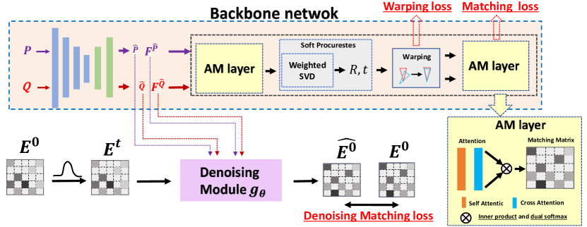
Our framework utilize a KPConv[9] branch to give the downsampled the superpoints $\hat{P}$ and $\hat{Q}$ and the asccociated features $F^{\hat{P}}$ and $F^{\hat{Q}}$. After that, we utilize a repositioning transformer[5] to predict the matching matrix and transformation $R,t$. This matching matrix and transformation are supervised by the Matching loss $L_{M}$ and Warping loss $L_{W}$ from [5]. To train the denoising module, we utilize the Gaussian transition kernel to add noise to the ground truth matching matrix $E^{0}$ to make $E^{t}$ at timestamp $t$. Then we exploit focal loss to train the denoising module $g_{\theta}$. We exploit the focal loss $L_{simple}$ (which is the denoising matching term in Eqn.16) to optimize $g_{\theta}$. The total loss is defined as:

$$L=L_{M}+L_{W}+L_{simple}$$ (26)

Figure 3: Overview of our framework training. Our framework includes a KPConv[9] featuren backbone optimization and a denoising module optimization. The training detail of the denoising module is listed in Algorithm.2. We implement the denoising matching loss $L_{simple}$ by utilizing a focal loss. After the model has been trained, only the KPConv[9] backbone and denoising module remain for use in the reverse sampling process, while the other components are discarded.

IV Experiments

IV-A Implementation Details.

For backbone network design, we follow Lepard [5] in our implementation. The dimension $d$ of superpoint features $F^{\hat{P}}$ and $F^{\hat{Q}}$ is set as $d=528$. Inspired by [5], we also utilize the rotationary position embedding for the denoising transformer and the matching function. Our proposed model is trained and tested with PyTorch on one NVIDIA RTX 3090 GPU. We train our model about 30 epochs on 3DMatch and 4DMatch with batch size 2. We follow the training/validation/test split strategy in Predator[29] and Lepard[5] for 3DMatch and 4DMatch, respectively. We conduct 20 iterations in the reverse denoising sampling process, while the total diffusion step number is set to 1000.

IV-B Rigid datasets: 3DMatch and 3DLoMatch

IV-B1 Datasets.

3DMatch[52] is an indoor benchmark for 3D matching and registration. Following[29, 4, 5], we split it to 46/8/8 for training/validation/testing. The overlap ratio between scan pairs in 3DMatch/3DLoMatch is about $>30\%$/$10\%-30\%$.

IV-B2 Metrics.

Following[29, 4, 53], we utilize three evaluation metrics to evaluate our method and other baselines: (1) Inlier Ratio (IR): The proportion of accurate correspondences in which the distance falls below a threshold (i.e., $0.1m$) based on the ground truth transformation. (2) Feature Matching Recall (FMR): The percentage of matched pairs that have an inlier ratio exceeding a specified threshold (i.e., $5\%$). (3) Registration Recall (RR): The fraction of successfully registered point cloud pairs with a predicted transformation error below a certain threshold (e.g., RMSE $<$ 0.2).

IV-B3 Results.

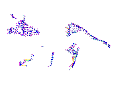
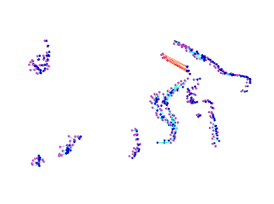
We compare our method with some state-of-the-art feature matching based methods: FCGF [54], D3Feat[28], Predator[29], and Lepard[5]. For the sake of fairness and unity, we utilize the RANSAC to give the registration results. As shown in the TABLE.I, our method achieves the best registration recall. In Fig.4, we found that our method can offer more reliable candidate correspondences for the RANSAC process.

(a) Lepard [5]

(b) Ours

(c) Lepard [5]

(d) Ours

Figure 4: The qualitative results of rigid registration in the 3DMatch/3DLoMatch benchmark. Zoom in for details.

TABLE I: Quantitative results on the 3DMatch and 3DLoMatch benchmarks. The best results are highlighted in bold, and the second-best results are underlined.

Method	3DMatch			3DLoMatch
	FMR	IR	RR	FMR	IR	RR
FCGF[54]	95.20	56.90	88.20	60.90	21.40	45.80
D3Feat[28]	95.80	39.00	85.80	69.30	13.20	40.20
Predator[29]	96.70	58.00	91.80	78.60	26.70	62.40
Lepard[5]	97.95	57.61	93.90	84.22	27.83	70.63
GeoTR[4]	98.1	72.7	92.3	88.7	44.7	75.4
RoITr[31]	98.0	82.6	91.9	89.6	54.3	74.8
Ours(Diff-PCR)	97.41	55.61	94.25	80.59	22.54	73.39

TABLE II: Quantitative results on the 4DMatch and 4DLoMatch benchmarks. The best results are highlighted in bold, and the second-best results are underlined. S denotes if it is a supervised method.

Category	Method	S	4DMatch		4DLoMatch
			NFMR	IR	NFMR	IR
Scene Flow	PointPWC [55]	✓	21.6	20.0	10.0	7.2
	FLOT [56]	✓	27.1	24.9	15.2	10.7
	NSFP[57]		18.5	16.3	1.2	0.5
Feature Matching	D3Feat [28]	✓	55.5	54.7	27.4	21.5
	Predator [29]	✓	56.4	60.4	32.1	27.5
	Lepard [5]	✓	83.60	82.64	66.63	55.55
	GeoTR[4]	✓	83.2	82.2	65.4	63.6
	RoITr[31]	✓	83.0	84.4	69.4	67.6
	Ours(Diff-PCR)	✓	88.39	86.40	76.23	67.80

TABLE III: The ablay study of initialization for the reverse sampling process. $E^{T}_{Backbone}$ denote the $E^{T}$ is generated by the backbone’s output. $E^{T}_{Gaussian}$ denote the $E^{T}$ is sampling from the Gaussian white noise $N(0,1)^{N{\times}M}$.

	3DMatch			3DLoMatch
	FMR	IR	RR	FMR	IR	RR
$E^{T}_{Backbone}$	97.23	55.61	94.23	83.01	23.69	72.55
$E^{T}_{Gaussian}$	97.41	55.61	94.25	80.59	22.54	73.39
	4DMatch			4DLoMatch
	NFMR	IR		NFMR	IR
$E^{T}_{Backbone}$	88.38	86.38		75.94	67.64
$E^{T}_{Gaussian}$	88.40	86.40		76.09	67.73

TABLE IV: This result of reverse sampling process in deterministic DDIM (i.e., $z_{t}=0$ in Eqn.15). $Backbone$ denotes the $E^{T}$ generated by the backbone’s output. $Gaussian$ denote the $E^{T}$ is sampled from the Gaussian white noise $N(0,1)^{N{\times}M}$.

	3DMatch			3DLoMatch
	FMR	IR	RR	FMR	IR	RR
$E^{T}_{Gaussian}$	97.66	58.86	94.27	83.79	27.26	73.80
$E^{T}_{Backbone}$	97.66	58.82	94.13	83.79	27.26	73.89
	4DMatch			4DLoMatch
	NFMR	IR		NFMR	IR
$E^{T}_{Gaussian}$	88.34	86.36		76.22	67.82
$E^{T}_{Backbone}$	88.72	86.72		76.48	68.16

TABLE V: Non-rigid registration results of 4DMatch/4DLoMatch. By utilizing correspondences generated from our method, we conduct the non-rigid registration by utilizing deformable registration method NDP[50].

Method	4DMatch-F				4DLoMatch-F
	EPE$\downarrow$	AccS$\uparrow$	AccR$\uparrow$	Outlier$\downarrow$	EPE$\downarrow$	AccS$\uparrow$	AccR$\uparrow$	Outlier$\downarrow$
PointPWC[55]	0.182	6.25	21.49	52.07	0.279	1.69	8.15	55.70
FLOT[56]	0.133	7.66	27.15	40.49	0.210	2.73	13.08	42.51
GeomFmaps [9]	0.152	12.34	32.56	37.90	0.148	1.85	6.51	64.63
Synorim-pw [19]	0.099	22.91	49.86	26.01	0.170	10.55	30.17	31.12
Lepard$+$NICP[5]	0.097	51.93	65.32	23.02	0.283	16.80	26.39	52.99
Lepard$+$NDP[50]	0.075	62.85	75.26	16.78	0.169	28.65	43.37	32.14
Ours(Diff-PCR)$+$NDP	0.062	65.52	78.75	13.84	0.141	32.29	48.96	25.75

IV-C Non-Rigid datasets: 4DMatch and 4DLoMatch

IV-C1 Datasets.

4DMatch/4DLoMatch[5] is an benchmark generated by the animation sequences from DeformingThings4D[58]. We follow the dataset split provided in [5], which has a wide range of overlap ratio, that $45\%$-$92\%$ in 4DMatch and $15\%$-$45\%$ in 4DLoMatch.

IV-C2 Metrics.

Following Lepard[5], we utilize two evaluation metrics to evaluate the quality of predicted matches. (1) Inlier ratio (IR): This measure denotes the correct fraction in the correspondences prediction $\mathcal{K}_{pred}$. We define it as:

$$IR=\frac{1}{|\mathcal{K}_{pred}|}\Sigma_{(p,q)\in\mathcal{K}_{pred}}[||W_{gt}(p)-q||_{2}<\sigma]$$ (27)

where $||\cdot||_{2}$ is the Euclidean norm, $W_{gt}(\cdot)$ is the ground truth warping function, $[\cdot]$ is the Inverse bracket, and $\sigma=0.04m$. (2) Non-rigid Feature Matching Recall (NFMR): This measure is to compute the fraction of the ground truth correspondences $(u,v)\in\mathcal{K}_{gt}$ that can be successfully recovered from the predicted correspondences $\mathcal{K}_{pred}$. First, we construct the predicted correspondences $\mathcal{A}=\{p|(p,q)\in\mathcal{K}_{pred}\}$ and the associated sparse 3D flow fields $\mathcal{F}=\{q-p|(p,q)\in\mathcal{K}_{pred}\}$. Then, for any source point $u$ in $\mathcal{K}_{gt}$, we can recover the flow field for $u$ by inverse distance interpolation:

$$\Gamma(u,\mathcal{A},\mathcal{F})=\Sigma_{\mathcal{A}_{i}\in knn(u,\mathcal{A})}\frac{\mathcal{F}_{i}||u-\mathcal{A}_{i}||^{-1}}{\Sigma_{\mathcal{A}_{i}\in knn(u,\mathcal{A})}||u-\mathcal{A}_{i}||_{2}^{-1}}$$ (28)

where $knn(\cdot,\cdot)$ is k-nearest neighbors search with k = 3. After that, we define the $NFMR$ to measure the fraction of ground truth matches that we discovered from $\mathcal{K}_{pred}$:

$$NFMR=\frac{1}{|\mathcal{K}_{gt}|}[||\Gamma(u,\mathcal{A},\mathcal{F})-v||_{2}<\sigma]$$ (29)

(a)

(b)

(c)

(d)

(e)

(f)

(g)

(h)

Figure 5: The qualitative results of deformable matching in the 4DMatch/4DLoMatch benchmark. The top results are generated by Lepard[5]. The bottom results are from our method. The red/green denotes two directions matching errors. Zoom in for details.

(a) Step=0

(b) Step=5

(c) Step=10

(d) Step=15

(e) Step=20

Figure 6: An example of the reverse sampling process. The red/green denotes two directions matching errors. Zoom in for details.

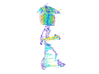
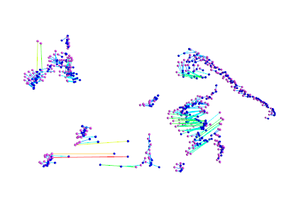
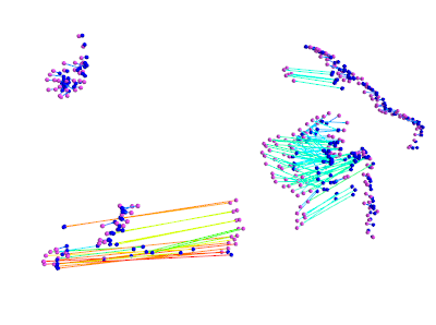
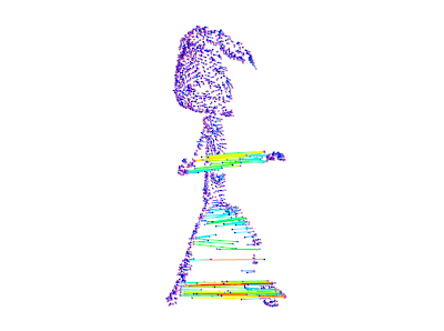
IV-C3 Results.

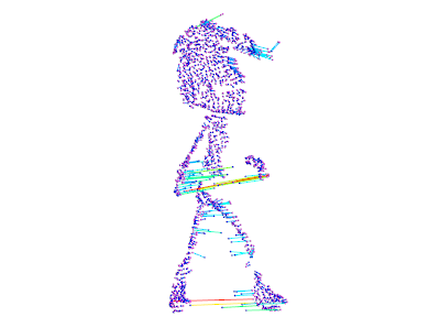
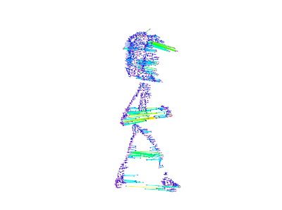
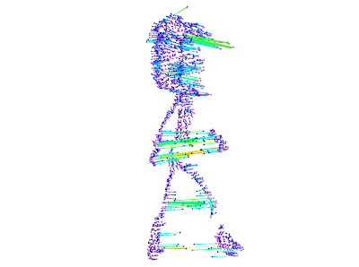
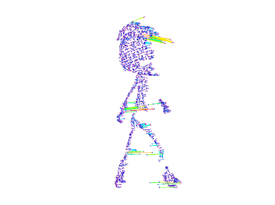
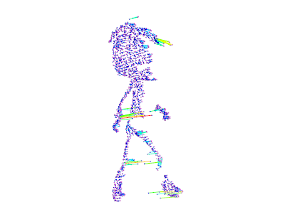
We compare our method with two categories of state-of-the-art methods. The first category includes Scene Flow Methods such as PWC[55], FLOT[56], and NSFP[57]. The second category encapsulates Feature Matching-Based Methods, namely D3Feat[28], Predator[29], Lepard[5]. As depicted in TABLE.II, our method realizes significant improvements compared with the baseline model Lepard[5]. We provide a visualization to demonstrate our method’s effectiveness in Fig.5. The red/green representation denotes the two-directional error. Our denoising optimizer indeed mitigates matching errors across different overlap ratios.

Figure 7: The qualitative results of non-rigid registration in the 4DMatch/4DLoMatch benchmark. The top four are generated by Lepard+NDP[50], while the bottom four are generated by Ours+NDP[50]. NDP[50] is a recent state-of-the-art non-registration method. Zoom in for details.

IV-D Ablation Studies and Discussions.

IV-D1 The Denoising Transformer Design.

In this paper, we have empirically observed that the integration of KPConv [9] as a backbone in a simple transformer has already shown remarkable performance improvement compared to other state-of-the-art point cloud registration methods. Recently, there have been numerous studies exploring various feature embedding networks for designing denoising modules, all of which have resulted in improved performances. Moreover, we can further enhance the performance by incorporating more powerful transformers specifically designed for registration tasks and integrating semantic or geometric prior knowledge [4, 16]. For example, in the case of rigid registration, we can incorporate GeoTR [4] or the semantic-enhanced geometric transformer [7] into $f_{\theta}$. The enhancement of the denoising feature embedding network will be addressed in future work. In this paper, we utilize the standard attention layer (integrated with rotationary position embedding[5]) as our denoising point feature embedding, which supports feature embedding in both rigid and non-rigid registration scenarios.

IV-D2 Reverse Sampling Initialization Choice.

The DDPM framework is specifically designed for removing noise from perturbed samples. Typically, we start with a baseline method that provides a reasonably satisfactory solution, which can then be further refined to achieve better performance. To demonstrate that our denoising network has indeed learned the optimization gradient regardless of the starting point, we conducted an ablative experiment. In this experiment, we initiated reverse sampling from the solution obtained by a pre-trained backbone or from Gaussian white noise. The results of this experiment, as presented in TABLE.III, indicates that our denoising network is capable of starting from any initialization or even from white noise. It can perform subsequent reverse sampling and ultimately reach the optimal solution. This finding demonstrates the robustness and effectiveness of our denoising network in achieving desirable outcomes regardless of the starting conditions.

TABLE VI: The ablay study of the iterative steps of reverse sampling. $0^{*}$ denote the pretrained Lepard[5]’s results.

Iters	RR		NFMR/IR
	3DMatch	3DLoMatch	4DMatch	4DLoMatch
0∗	93.50	69.00	83.74/82.74	66.94/55.74
1	93.96	73.39	85.34/83.93	73.11/65.26
2	93.96	73.12	85.24/83.84	73.27/65.19
3	94.04	73.52	85.52/84.06	73.19/65.22
10	94.27	73.59	87.99/86.07	75.46/67.15
20	94.23	73.54	88.39/86.64	76.16/67.82
50	93.98	73.35	88.61/86.62	76.34/68.03
100	94.31	73.37	88.55/86.58	76.46/68.15
200	94.36	73.36	88.59/86.61	76.42/68.10

IV-D3 Reverse Sampling Steps.

In our approach, we consider the denoising module as an optimizer that searches for the optimal solution for the matching matrix. We argue that increasing the number of search iterations may lead to better solutions. To validate this hypothesis, we conducted an experiment to investigate the impact of iterative searching steps on the results. Table.VII presents the results of all the experiments, where the outcomes denoted by ”0*” correspond to the results obtained by Lepard[5] without any denoising steps. We ran the reverse sampling step from 1 to 200 iterations. As shown in Table V, the registration recall of our method consistently increases as the number of searching steps grows. This behavior is different from other iterative methods[5], which often experience performance degradation after a certain number of iterations. Even with just one iteration, our method achieves significant performance improvement, demonstrating the effectiveness of the denoising optimizer. These results provide evidence that increasing the number of search steps can lead to improved performance in our approach. We also illustrate a case (see Fig.6) where the matching error gradually decreases with more sampling steps.

IV-D4 Deterministic Sampling vs Non-deterministic Sampling

Several empirical studies[34, 40] have observed that deterministic sampling tends to perform better compared to the original DDPM reverse sampling. To investigate this, we conducted an experiment and observed a slight difference in performance between these two strategies. The results presented in TABLE IV are based on deterministic sampling, while the non-deterministic sampling results are shown in TABLE III for comparison. As indicated in TABLE IV, deterministic sampling does indeed yield slightly better results. One possible reason for this is that the Gaussian noise used in non-deterministic sampling may not be the optimal choice for achieving the best performance. It highlights the importance of carefully considering the sampling strategy and its impact on overall performance.

IV-E Integrating Correspondences to Non-rigid Registration

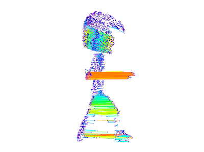
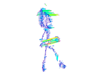
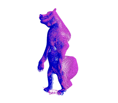
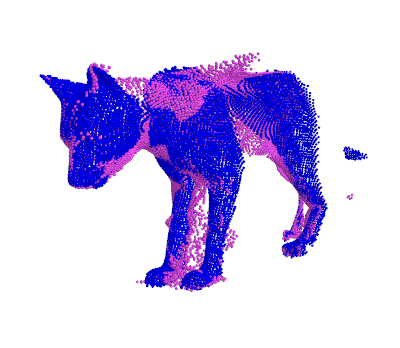
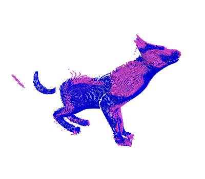
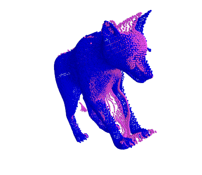
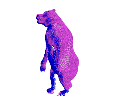
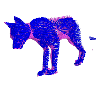
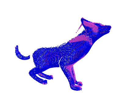
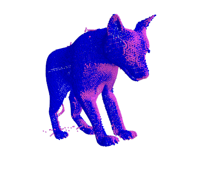
Given the correspondence from our method, we could conduct the non-rigid registration to showcase our method’s effectiveness. Since the 4DMatch dataset has many rigid movements dominating examples, following NDP[50], we remove the near-rigid movement examples, and we denote the filtered datasets as 4DMatch-F/4DLoMatch-F. Since we utilize the rigid warping in our denoising module, to prove the effectiveness of our current version design, we conduct the non-rigid registration experiments on 4DMatch-F/4DLoMatch-F datasets. We utilize the NDP[50] as our non-rigid registration framework. As illustrated in TABLE.V, the correspondences generated by our method can improve the performance of deformable registration. We also provide a visual analysis in Fig.7. The top line is generated by Lepard[5]’s correspondences and NDP[50]’s deformable registration, while the bottom line is generated by ours+NDP. Due to the sampling of the matching matrix constraint in the doubly stochastic matrix manifolds, our method can better predict the matches between symmetrical front legs and reduce adhesion.

TABLE VII: Comparison of time cost in the iterative step ( or the reverse sampling step).

Iters	3DMatch		3DLoMatch
	RR	Time(sec.)	RR	Time(sec.)
GeoTR[4]	92.0	0.296	74.0	0.284
GeoTR. + PEAL[16] 1-step	93.7	0.663	77.8	0.642
GeoTR. + DiffusionPCR[34] 1-step	93.9	0.625	78.2	0.620
KPConv. + Diff-PCR 1-step	93.96	0.032	73.39	0.036
GeoTR. + PEAL[16] 5-step	94.0	2.131	78.5	2.074
GeoTR. + DiffusionPCR[34] 5-step	94.4	1.939	80.0	1.964
KPConv. + Diff-PCR 5-step	94.13	0.095	73.78	0.098

IV-F The lightweight design of our denoising module

Due to its lightweight design, our denoising network exhibits a significant speed improvement compared to other diffusion-based methods employed for point cloud registration. This enhancement allows our approach to execute a greater number of denoising iterations. We have included a detailed list showcasing the time costs (see TABLE.VII) associated with each reverse denoising step, as well as comparisons to recent works. Under our lightweight design, our method achieves competitive results on the 3DMatch benchmark. If we utilize the GeoTR as our denoising transformer, our method will achieve at least the same performance in the 3DLoMatch benchmark, and save about 0.025 seconds (which is the time cost for KPConv backbone embedding) for each iterative step. We leave this improvement on the 3DLoMatch in future work.

V Conclusion

This paper introduces a novel framework that utilizes a diffusion model in the Doubly Stochastic Matrix Space to learn a gradient for guiding the search toward the optimal matching matrix solution. Additionally, we incorporate a lightweight design for the denoising module, which helps reduce the time cost of iterative reverse sampling. Experimental results on both rigid and non-rigid datasets validate the effectiveness and efficiency of our proposed framework.

References

- [1] X. Huang, G. Mei, J. Zhang, and R. Abbas, “A comprehensive survey on point cloud registration,” 2021.
- [2] Y. Shen, L. Hui, J. Xie, and J. Yang, “Self-supervised 3d scene flow estimation guided by superpoints,” in Proceedings of the IEEE/CVF Conference on Computer Vision and Pattern Recognition, 2023, pp. 5271–5280.
- [3] J. Zhang and S. Singh, “Loam: Lidar odometry and mapping in real-time.” in Robotics: Science and systems, vol. 2, no. 9. Berkeley, CA, 2014, pp. 1–9.
- [4] Z. Qin, H. Yu, C. Wang, Y. Guo, Y. Peng, and K. Xu, “Geometric transformer for fast and robust point cloud registration,” in Proceedings of the IEEE/CVF Conference on Computer Vision and Pattern Recognition, 2022, pp. 11 143–11 152.
- [5] Y. Li and T. Harada, “Lepard: Learning partial point cloud matching in rigid and deformable scenes,” in Proceedings of the IEEE/CVF Conference on Computer Vision and Pattern Recognition, 2022, pp. 5554–5564.
- [6] Z. J. Yew and G. H. Lee, “Regtr: End-to-end point cloud correspondences with transformers,” in Proceedings of the IEEE/CVF Conference on Computer Vision and Pattern Recognition, 2022, pp. 6677–6686.
- [7] Q. Wu, Y. Ding, L. Luo, C. Zhou, J. Xie, and J. Yang, “Sgfeat: Salient geometric feature for point cloud registration,” arXiv preprint arXiv:2309.06207, 2023.
- [8] G. Mei, H. Tang, X. Huang, W. Wang, J. Liu, J. Zhang, L. Van Gool, and Q. Wu, “Unsupervised deep probabilistic approach for partial point cloud registration,” in Proceedings of the IEEE/CVF Conference on Computer Vision and Pattern Recognition, 2023, pp. 13 611–13 620.
- [9] H. Thomas, C. R. Qi, J.-E. Deschaud, B. Marcotegui, F. Goulette, and L. J. Guibas, “Kpconv: Flexible and deformable convolution for point clouds,” in Proceedings of the IEEE/CVF international conference on computer vision, 2019, pp. 6411–6420.
- [10] X. Bai, Z. Luo, L. Zhou, H. Chen, L. Li, Z. Hu, H. Fu, and C.-L. Tai, “Pointdsc: Robust point cloud registration using deep spatial consistency,” in Proceedings of the IEEE/CVF Conference on Computer Vision and Pattern Recognition, 2021, pp. 15 859–15 869.
- [11] Z. Chen, K. Sun, F. Yang, and W. Tao, “Sc2-pcr: A second order spatial compatibility for efficient and robust point cloud registration,” in Proceedings of the IEEE/CVF Conference on Computer Vision and Pattern Recognition, 2022, pp. 13 221–13 231.
- [12] C. R. Qi, O. Litany, K. He, and L. J. Guibas, “Deep hough voting for 3d object detection in point clouds,” in proceedings of the IEEE/CVF International Conference on Computer Vision, 2019, pp. 9277–9286.
- [13] Z. Qin, H. Yu, C. Wang, Y. Peng, and K. Xu, “Deep graph-based spatial consistency for robust non-rigid point cloud registration,” in Proceedings of the IEEE/CVF Conference on Computer Vision and Pattern Recognition, 2023, pp. 5394–5403.
- [14] H. Jiang, Z. Dang, Z. Wei, J. Xie, J. Yang, and M. Salzmann, “Robust outlier rejection for 3d registration with variational bayes,” in Proceedings of the IEEE/CVF Conference on Computer Vision and Pattern Recognition, 2023, pp. 1148–1157.
- [15] X. Zhang, J. Yang, S. Zhang, and Y. Zhang, “3d registration with maximal cliques,” in Proceedings of the IEEE/CVF Conference on Computer Vision and Pattern Recognition, 2023, pp. 17 745–17 754.
- [16] J. Yu, L. Ren, Y. Zhang, W. Zhou, L. Lin, and G. Dai, “Peal: Prior-embedded explicit attention learning for low-overlap point cloud registration,” in Proceedings of the IEEE/CVF Conference on Computer Vision and Pattern Recognition, 2023, pp. 17 702–17 711.
- [17] X. Gu, C. Tang, W. Yuan, Z. Dai, S. Zhu, and P. Tan, “Rcp: Recurrent closest point for scene flow estimation on 3d point clouds,” arXiv preprint arXiv:2205.11028, 2022.
- [18] Z. Teed and J. Deng, “Raft: Recurrent all-pairs field transforms for optical flow,” in Computer Vision–ECCV 2020: 16th European Conference, Glasgow, UK, August 23–28, 2020, Proceedings, Part II 16. Springer, 2020, pp. 402–419.
- [19] G. Mei, X. Huang, L. Yu, J. Zhang, and M. Bennamoun, “Cotreg: Coupled optimal transport based point cloud registration,” arXiv preprint arXiv:2112.14381, 2021.
- [20] Q. Wu, Y. Shen, H. Jiang, G. Mei, Y. Ding, L. Luo, J. Xie, and J. Yang, “Graph matching optimization network for point cloud registration.”
- [21] J. Ho, A. Jain, and P. Abbeel, “Denoising diffusion probabilistic models,” Advances in neural information processing systems, vol. 33, pp. 6840–6851, 2020.
- [22] M. Jaggi, “Revisiting frank-wolfe: Projection-free sparse convex optimization,” in International Conference on Machine Learning. PMLR, 2013, pp. 427–435.
- [23] G. Parisi, “Correlation functions and computer simulations,” Nuclear Physics B, vol. 180, no. 3, pp. 378–384, 1981.
- [24] R. M. Neal et al., “Mcmc using hamiltonian dynamics,” Handbook of markov chain monte carlo, vol. 2, no. 11, p. 2, 2011.
- [25] R. M. Caron, X. Li, P. Mikusiński, H. Sherwood, and M. D. Taylor, “Nonsquare ”doubly stochastic” matrices,” Lecture Notes-Monograph Series, vol. 28, pp. 65–75, 1996. [Online]. Available: http://www.jstor.org/stable/4355884
- [26] Z. Teed and J. Deng, “Raft-3d: Scene flow using rigid-motion embeddings,” in Proceedings of the IEEE/CVF conference on computer vision and pattern recognition, 2021, pp. 8375–8384.
- [27] J. Song, C. Meng, and S. Ermon, “Denoising diffusion implicit models,” arXiv preprint arXiv:2010.02502, 2020.
- [28] X. Bai, Z. Luo, L. Zhou, H. Fu, L. Quan, and C.-L. Tai, “D3feat: Joint learning of dense detection and description of 3d local features,” in Proceedings of the IEEE/CVF conference on computer vision and pattern recognition, 2020, pp. 6359–6367.
- [29] S. Huang, Z. Gojcic, M. Usvyatsov, A. Wieser, and K. Schindler, “Predator: Registration of 3d point clouds with low overlap,” in Proceedings of the IEEE/CVF Conference on computer vision and pattern recognition, 2021, pp. 4267–4276.
- [30] H. Yu, F. Li, M. Saleh, B. Busam, and S. Ilic, “Cofinet: Reliable coarse-to-fine correspondences for robust pointcloud registration,” Advances in Neural Information Processing Systems, vol. 34, pp. 23 872–23 884, 2021.
- [31] H. Yu, Z. Qin, J. Hou, M. Saleh, D. Li, B. Busam, and S. Ilic, “Rotation-invariant transformer for point cloud matching,” in Proceedings of the IEEE/CVF Conference on Computer Vision and Pattern Recognition, 2023, pp. 5384–5393.
- [32] H. Yu, J. Hou, Z. Qin, M. Saleh, I. Shugurov, K. Wang, B. Busam, and S. Ilic, “Riga: Rotation-invariant and globally-aware descriptors for point cloud registration,” arXiv preprint arXiv:2209.13252, 2022.
- [33] H. Deng, T. Birdal, and S. Ilic, “Ppf-foldnet: Unsupervised learning of rotation invariant 3d local descriptors,” in Proceedings of the European Conference on Computer Vision (ECCV), 2018, pp. 602–618.
- [34] Z. Chen, Y. Ren, T. Zhang, Z. Dang, W. Tao, S. Süsstrunk, and M. Salzmann, “Diffusionpcr: Diffusion models for robust multi-step point cloud registration,” arXiv preprint arXiv:2312.03053, 2023.
- [35] Y. Song and S. Ermon, “Generative modeling by estimating gradients of the data distribution,” Advances in neural information processing systems, vol. 32, 2019.
- [36] S. Chen, P. Sun, Y. Song, and P. Luo, “Diffusiondet: Diffusion model for object detection,” in Proceedings of the IEEE/CVF International Conference on Computer Vision, 2023, pp. 19 830–19 843.
- [37] J. Austin, D. D. Johnson, J. Ho, D. Tarlow, and R. Van Den Berg, “Structured denoising diffusion models in discrete state-spaces,” Advances in Neural Information Processing Systems, vol. 34, pp. 17 981–17 993, 2021.
- [38] S. Gu, D. Chen, J. Bao, F. Wen, B. Zhang, D. Chen, L. Yuan, and B. Guo, “Vector quantized diffusion model for text-to-image synthesis,” in Proceedings of the IEEE/CVF Conference on Computer Vision and Pattern Recognition, 2022, pp. 10 696–10 706.
- [39] J. Urain, N. Funk, J. Peters, and G. Chalvatzaki, “Se (3)-diffusionfields: Learning smooth cost functions for joint grasp and motion optimization through diffusion,” in 2023 IEEE International Conference on Robotics and Automation (ICRA). IEEE, 2023, pp. 5923–5930.
- [40] H. Jiang, M. Salzmann, Z. Dang, J. Xie, and J. Yang, “Se (3) diffusion model-based point cloud registration for robust 6d object pose estimation,” arXiv preprint arXiv:2310.17359, 2023.
- [41] J. N. Sohl-Dickstein, E. A. Weiss, N. Maheswaranathan, and S. Ganguli, “Deep unsupervised learning using nonequilibrium thermodynamics,” ArXiv, vol. abs/1503.03585, 2015. [Online]. Available: https://api.semanticscholar.org/CorpusID:14888175
- [42] Y. Song, J. Sohl-Dickstein, D. P. Kingma, A. Kumar, S. Ermon, and B. Poole, “Score-based generative modeling through stochastic differential equations,” arXiv preprint arXiv:2011.13456, 2020.
- [43] D. P. Kingma, T. Salimans, B. Poole, and J. Ho, “Variational diffusion models,” ArXiv, vol. abs/2107.00630, 2021. [Online]. Available: https://api.semanticscholar.org/CorpusID:235694314
- [44] M. Cuturi, “Sinkhorn distances: Lightspeed computation of optimal transport,” Advances in neural information processing systems, vol. 26, 2013.
- [45] P. J. Besl and N. D. McKay, “Method for registration of 3-d shapes,” in Sensor fusion IV: control paradigms and data structures, vol. 1611. Spie, 1992, pp. 586–606.
- [46] S. Bond-Taylor, P. Hessey, H. Sasaki, T. P. Breckon, and C. G. Willcocks, “Unleashing transformers: Parallel token prediction with discrete absorbing diffusion for fast high-resolution image generation from vector-quantized codes,” in European Conference on Computer Vision. Springer, 2022, pp. 170–188.
- [47] K. S. Arun, T. S. Huang, and S. D. Blostein, “Least-squares fitting of two 3-d point sets,” IEEE Transactions on pattern analysis and machine intelligence, no. 5, pp. 698–700, 1987.
- [48] R. W. Sumner, J. Schmid, and M. Pauly, “Embedded deformation for shape manipulation,” in ACM siggraph 2007 papers, 2007, pp. 80–es.
- [49] T. Igarashi, T. Moscovich, and J. F. Hughes, “As-rigid-as-possible shape manipulation,” ACM transactions on Graphics (TOG), vol. 24, no. 3, pp. 1134–1141, 2005.
- [50] Y. Li and T. Harada, “Non-rigid point cloud registration with neural deformation pyramid,” Advances in Neural Information Processing Systems, vol. 35, pp. 27 757–27 768, 2022.
- [51] A. Vaswani, N. Shazeer, N. Parmar, J. Uszkoreit, L. Jones, A. N. Gomez, Ł. Kaiser, and I. Polosukhin, “Attention is all you need,” Advances in neural information processing systems, vol. 30, 2017.
- [52] A. Zeng, S. Song, M. Nießner, M. Fisher, J. Xiao, and T. Funkhouser, “3dmatch: Learning local geometric descriptors from rgb-d reconstructions,” in Proceedings of the IEEE conference on computer vision and pattern recognition, 2017, pp. 1802–1811.
- [53] J. Lee, M. Cho, and K. M. Lee, “Hyper-graph matching via reweighted random walks,” in CVPR 2011. IEEE, 2011, pp. 1633–1640.
- [54] C. Choy, J. Park, and V. Koltun, “Fully convolutional geometric features,” in Proceedings of the IEEE/CVF International Conference on Computer Vision, 2019, pp. 8958–8966.
- [55] W. Wu, Z. Wang, Z. Li, W. Liu, and L. Fuxin, “Pointpwc-net: A coarse-to-fine network for supervised and self-supervised scene flow estimation on 3d point clouds,” arXiv preprint arXiv:1911.12408, 2019.
- [56] G. Puy, A. Boulch, and R. Marlet, “Flot: Scene flow on point clouds guided by optimal transport,” in European conference on computer vision. Springer, 2020, pp. 527–544.
- [57] X. Li, J. Kaesemodel Pontes, and S. Lucey, “Neural scene flow prior,” Advances in Neural Information Processing Systems, vol. 34, pp. 7838–7851, 2021.
- [58] Y. Li, H. Takehara, T. Taketomi, B. Zheng, and M. Nießner, “4dcomplete: Non-rigid motion estimation beyond the observable surface,” in Proceedings of the IEEE/CVF International Conference on Computer Vision, 2021, pp. 12 706–12 716.