Client-wise Modality Selection for Balanced Multi-modal Federated Learning

Abstract

Selecting proper clients to participate in the iterative federated learning (FL) rounds is critical to effectively harness a broad range of distributed datasets. Existing client selection methods simply consider the variability among FL clients with uni-modal data, however, have yet to consider clients with multi-modalities. We reveal that traditional client selection scheme in MFL may suffer from a severe modality-level bias, which impedes the collaborative exploitation of multi-modal data, leading to insufficient local data exploration and global aggregation. To tackle this challenge, we propose a Client-wise Modality Selection scheme for MFL (CMSFed) that can comprehensively utilize information from each modality via avoiding such client selection bias caused by modality imbalance. Specifically, in each MFL round, the local data from different modalities are selectively employed to participate in local training and aggregation to mitigate potential modality imbalance of the global model. To approximate the fully aggregated model update in a balanced way, we introduce a novel local training loss function to enhance the weak modality and align the divergent feature spaces caused by inconsistent modality adoption strategies for different clients simultaneously. Then, a modality-level gradient decoupling method is designed to derive respective submodular functions to maintain the gradient diversity during the selection progress and balance MFL according to local modality imbalance in each iteration. Our extensive experiments showcase the superiority of CMSFed over baselines and its effectiveness in multi-modal data exploitation.

1 Introduction

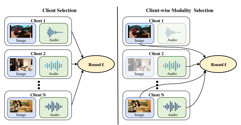
Figure 1: Traditional client selection in FL aims to sample a client subset in each round. The selected clients use all their local data for training and aggregation. To exploit different modalities comprehensively, we propose the client-wise modality selection for MFL, which considers the local data from each modality as the sampling unit rather than the client. Only the selected modality data from a client would join in training and aggregation.

Federated learning (FL) [20] aims to collaboratively learn data that has been collected by, and resides on, a number of remote devices or servers. FL stands to develop top-performing models by aggregating knowledge from numerous edge clients [6], which relies on the iterative interaction among participating clients and the server. However, comprehensively employing the information from all clients can be exceptionally difficult due to the client heterogeneity and resource limitations [8, 27].

Random sampling [32, 19] from available clients is widely used in FL to satisfy some practical restrictions, e.g., limited communication bandwidth [23, 31] and computing capacities [13]. To improve the information exploitation of all clients, extensive research has been conducted on effective client selection strategies. One viable solution [24] is to gather as much local data as possible in each round while in contrast, some alternative studies [1] focus on collecting representative information by sampling a subset of clients. However, previous methods have only considered the knowledge discrepancies across different clients, while demonstrating notable performance in uni-modal FL, yet, their effectiveness diminishes when dealing with clients with multi-modal data as the inter-modality interactions during the FL training is neglected. The investigation into fine-grained and sophisticated data selection mechanism for multi-modal FL (MFL) is currently under-explored.

In this paper, we reveal that traditional client selection approaches may suffer from a severe modality-level bias in MFL. Due to the inconsistent learning progress of different modalities, i.e., the modality imbalance, client-level selection bias tends to favor information from a dominant modality while deprioritize the weak modality, which impedes the collaborative exploitation of distributed multi-modal data, leading to insufficient local data exploration and global aggregation.

To address such issue in MFL, we propose a novel Client-wise Modality Selection scheme for MFL (CMSFed), which chooses the appropriate modalities combination from clients in each round to alleviate the modality-level bias and realize full exploitation of each modality via considering the interactions between different modalities as illustrated in Fig. 1. Only part of, not all, modalities, will be selected for some clients compared with traditional client selection. Specifically, in each communication round, we intend to gather a data subset by selectively employing different modalities from each client, the aggregated model update stemmed from that approximates the fully aggregated update which fulfills the potential of each modality. Inspired from [1] for diverse client selection, we build the modality selection formula, namely the min-form of the facility location function [5] evaluated on the collected data subset, to seek for the representative information for the global model. To further release the ability of each modality and reduce the training cost, we propose a modality-level gradient decoupling with a modal-balanced local training loss to build two separated submodular functions and then modulate their optimization process for unbiased modality selection. As a result, inconsistent modality adoption strategies may lead to different feature spaces for different clients, which exacerbates the difficulties in accomplishing an accurate and generalized aggregated model. Therefore, the global prototype is introduced for the weak modality to alleviate the heterogeneous feature spaces. To summarize, our contributions in this paper are as follows:

• We scrutinize the client selection scheme in MFL and reveal that naive sampling clients may introduce a strong modality-level bias which causes insufficient utilization of multi-modal data.

• We propose a novel client-wise modality selection scheme for MFL (CMSFed) to comprehensively exploit all modalities via a enhancing loss and gradient decoupling to balance MFL.

• We conduct comprehensive experiments and demonstrate that 1) CMSFed can achieve considerable improvements over baselines; 2) CMSFed indeed achieves a more balanced exploitation of distributed multimodal data.

2 Background and Related Works

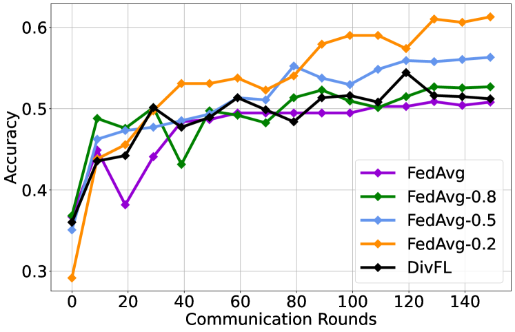
(a) Multi-modal

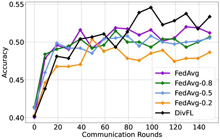
(b) Uni-audio

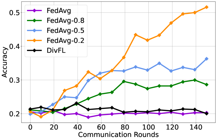
(c) Uni-visual

Figure 2: Performance of client selection strategies on CREMA-D with uniformly distributed data on 20 clients. FedAvg randomly selects clients while DivFL selects clients with diversity. ‘FedAvg-0.8’ means 80% of clients have data in both audio and visual modalities, while 20% of clients only have data in random one modality. ‘-0.5’ and ‘-0.2’ follow the similar definition. (a) Performance of global multi-modal model. (b) Performance of global uni-audio model. (c) Performance of global uni-visual model.

2.1 Multi-modal federated learning

In MFL, each client may contain one or more modalities of data. Without loss of generality, we consider two input modalities, referred to as $A$ and $I$ in MFL. There are a set $V$ of $N$ clients, $V=\left[N\right]$, respectively owning datasets $\mathcal{D}_{i}=\left\{\boldsymbol{X}_{i}^{A},\boldsymbol{X}_{i}^{I},y\right\}$ composed of $n_{i}$ pair samples, $i\in\left[N\right]$. A typical federated learning objective is the average of each client’s local loss function:

$$\vspace{-8pt}\min f\left(\theta\right)=\sum_{k=1}^{N}{p_{k}F_{k}\left(\theta\right)}$$ (1)

where $\theta=\left\{\theta^{A},\theta^{I},\omega\right\}$ denotes the model parameters. $\theta^{A}$ and $\theta^{I}$ represent the parameters of encoders of modality $A$ and $I$. $\omega$ is the parameters of fusion classifier. $p_{k}$ is a pre-defined weight. $F_{k}$ is each client’s local loss.

Statistical heterogeneity [14, 17] is a widely concerned challenge in uni-modal FL. To tackle this issue, FedProx [18] uses a proximal term to stabilize model aggregation. FedProto [29] shares class prototypes to regularize the learning of local models. In MFL, modality incongruity [38, 37] (clients consist of different modalities combinations), as well as statistical heterogeneity [35], are all considered. Yu et al. [37] propose CreamFL to align the representations between different clients and different modalities via communicating knowledge on a public dataset. Chen et al. [3] introduce FedMSplit to split local models into several components and aggregate them by their correlations. However, they still focus on the heterogeneity, but ignore the interaction between private data of different modalities, which limits their information exploitation.

2.2 Client selection and submodular function

Client selection [7, 36] is a critical issue for FL especially when the communication cost with all devices is prohibitively high, which has been extensively studied in uni-modal FL. Cho et al. [4] propose Power-of-Choice to select clients with largets local loss. Balakrishnan et al. [1] propose to select a subset of clients with great diversity.

Diverse client selection via submodularity. Maximizing a submodular function is reported to improve the diversity and reduce the redundancy of a subset. This property makes it appropriate for client selection in FL. If a function $F$ is submodular, it should satisfy: given a finite ground set $V$ of size $N$, $F\left(A\cup\left\{v\right\}\right)-F\left(A\right)\geqslant F\left(B\cup\left\{v\right\}\right)-F\left(B\right)$, for any $A\subseteq B\subseteq V$ and $v\in V\backslash B$. The marginal utility of an element $v$ w.r.t. a subset $A$ is denoted as $F\left(v|A\right)=F\left(A\cup\left\{v\right\}\right)-F\left(A\right)$, which can represent the importance of $v$ to $A$. The client selection via submodular maximization can be expressed following [1]: find a subset $S$ of clients whose aggregated gradients can approximate the full aggregation from all clients:

$$\sum_{k\in\left[N\right]}{\nabla F_{k}\left(v^{k}\right)} =\sum_{k\in\left[N\right]}{\left[\nabla F_{k}\left(v^{k}\right)-\nabla F_{\sigma\left(k\right)}\left(v^{\sigma\left(k\right)}\right)\right]}$$ (2)

$$+\sum_{k\in S}{\gamma_{k}\nabla F_{k}\left(v^{k}\right)}$$

where $\sigma$ maps $V\rightarrow S$ and the gradient $\nabla F_{k}\left(v^{k}\right)$ from client $k$ is approximated by the gradient from a selected client $\sigma\left(k\right)\in S$. For $i\in S$, let $C_{i}\triangleq\left\{k\in V|\sigma\left(k\right)=i\right\}$, and therefore $\gamma_{i}\triangleq|C_{i}|$. Take the norms and apply triangular inequality after subtracting the second term from both sides, we can obtain a relaxed objective $G\left(S\right)$ for minimizing the approximation error:

$$\begin{split}&\left\|\sum_{k\in\left[N\right]}{\nabla F_{k}\left(v^{k}\right)}-\sum_{k\in S}{\gamma_{k}\nabla F_{k}\left(v^{k}\right)}\right\|\leqslant\\ &\sum_{k\in\left[N\right]}{\underset{i\in S}{\min}\left\|\nabla F_{k}\left(v^{k}\right)-\nabla F_{i}\left(v^{i}\right)\right\|\triangleq G\left(S\right)}\end{split}$$ (3)

Minimizing $G\left(S\right)$ can be seen as maximizing the well-known submodular function, i.e., the facility location function [5]. The submodular maximizing problem is NP-hard but can be approximated via the greedy [22] or stochastic greedy algorithm [21]:

$$S\leftarrow S\cup k^{*},$$ (4)

$$k^{*}\in \underset{k\in\mathrm{rand}\left(V\backslash S,\mathrm{size}=s\right)}{\mathrm{arg}\max}\left[\bar{G}\left(S\right)-\bar{G}\left(\left\{k\right\}\cup S\right)\right]$$

$\bar{G}$ represents a constant minus the negation of $G$.

Although these methods make great improvement in uni-modal FL, the selection strategy is under-explored in MFL and we reveal that traditional client selection approaches fall into a severe bias in MFL.

2.3 Imbalanced multi-modal learning

Modality imbalance indicates the inconsistent learning progress of different modalities in multi-modal learning [33, 12]. Peng et al. [26] propose OGM-GE to alleviate the inhibitory effect on weak modality by slowing down the dominant modality. Fan et al. [9] further build a non-parametric classifier by class centroids to adjust the update direction of weak modality. In this paper, we aim to power each modality of all clients by a meticulously designed modality selection strategy in each round of training.

3 Observations and Analysis

In this section, we analyze the behavior of different client sampling strategies in MFL and the interactions between different modalities. As shown in Fig. 2, we compare a well-designed client selection method (DivFL) with random sampling (FedAvg) on a multi-modal dataset. The results in Fig. 2(a) show that the improvement from DivFL is severely limited although it is terrific in uni-modal FL. The results about how each modality behaves are illustrated in Figs. 2(b) and 2(c). It is apparent that audio modality performs much better than visual modality and the optimised client selection options from DivFL generally focus on audio modality (audio performance of DivFL has significant improvement over FedAvg while no noticeable difference in visual).

The performance gap between audio and visual can be attributed to ‘modality imbalance’ [33], which indicates the inconsistent learning paces in different modalities. Therefore, the imbalance nature (multi-modal learning is dominated by the modality who learns fast) [34] in MFL leads to a strong modality-level selection bias, i.e., client selection strategies tend to select clients that make the dominant modality aggregation better but neglect the weak modality

To further analyze the interactions between different modalities, we randomly discard the data of one modality (audio or visual) on clients with certain probabilities (FedAvg-0.8, -0.5, -0.2) as demonstrated in Fig. 2(a). It is clear that randomly discarding one modality data for part of clients does not necessarily lead to performance degradation of the global model, but may bring performance improvement. The reason behind can be found in Figs. 2(b) and 2(c), where the gap between audio and visual modalities gradually narrows as the discarding probability increases until there is no stark disparity (in FedAvg-0.2). This phenomenon is consistent with the findings in [26]: the dominant modality hinders the learning process of weak modality. Therefore, the ability of visual modality is released and absorbed by the global model through aggregation when the audio data in some clients is abandoned.

The above analyses suggest that traditional client selection methods are not applicable in MFL due to the modality imbalance nature, and the potential of each modality can be further explored by engaging appropriate modalities in training. Therefore, we intend to design a new modality selection scheme in MFL to address the modality imbalance and information underutilization from different modalities.

4 Method

In this section, we introduce CMSFed, a diverse and balanced modality selection strategy to realize more efficient data utilization. We first derive a combinatorial objective for modality selection in MFL via the gradient approximation with the fully aggregated update. Then we propose a modality-level gradient decoupling with the enhancing gradient on weak modality to build two separated submodular functions and balance MFL.

4.1 Client-wise modality selection

Firstly, we rewrite Eq. 2 for MFL as:

$$\begin{split}&\sum_{k\in\left[N\right]}{\nabla F_{k}\left(v_{A}^{k},v_{I}^{k}\right)}=\sum_{k\in S}{\gamma_{k}\nabla F_{k}\left(v_{A}^{k},v_{I}^{k}\right)}+\\ &\sum_{k\in\left[N\right]}{\left[\nabla F_{k}\left(v_{A}^{k},v_{I}^{k}\right)-\nabla F_{\sigma\left(k\right)}\left(v_{A}^{\sigma\left(k\right)},v_{I}^{\sigma\left(k\right)}\right)\right]}\end{split}$$ (5)

where $v_{A}^{k}$ and $v_{I}^{k}$ indicate the corresponding modal data in client $k$.

The above equation is still the client selection formulation, while we could build the modality selection formula based on it as (data superscripts are omitted for simplicity):

$$\sum_{k\in\left[N\right]}{\nabla F_{k}\left(v_{A},v_{I}\right)}$$ (6)

$$=\sum_{k\in\left[N\right]}{\left[\begin{array}[]{c}\nabla F_{k}\left(v_{A},v_{I}\right)-\nabla F_{\sigma_{M}\left(k\right)}\left(v_{A},v_{I}\right)\\ -\nabla F_{\sigma_{A}\left(k\right)}\left(v_{A}\right)-\nabla F_{\sigma_{I}\left(k\right)}\left(v_{I}\right)\\ \end{array}\right]}$$

$$+\sum_{k\in S_{M}}{\gamma_{k}^{M}\nabla F_{k}\left(v_{A},v_{I}\right)}+\sum_{k\in S_{A}}{\gamma_{k}^{A}\nabla F_{k}\left(v_{A}\right)}$$

$$+\sum_{k\in S_{I}}{\gamma_{k}^{I}\nabla F_{k}\left(v_{I}\right)}$$

where $\sigma_{M}$, $\sigma_{A}$ and $\sigma_{I}$ map $V\rightarrow S_{M},S_{A},S_{I}$, the client sets who use multi-modal, $A$ modal, and $I$ modal data for training respectively, and $S_{M}\cap S_{A}=S_{A}\cap S_{I}=S_{M}\cap S_{I}=\oslash$. The full gradient aggregation is represented by the customized update from multi-modal and uni-modal clients. Assume modality $I$ is weak here, the relaxed objective for modality selection should be:

$$\left\|\begin{array}[]{c}\sum_{k\in\left[N\right]}{\nabla F_{k}\left(v_{A},v_{I}\right)}-\sum_{k\in S_{I}}{\gamma_{k}^{I}\nabla F_{k}\left(v_{I}\right)}\\ -\sum_{k\in S_{M}}{\gamma_{k}^{M}\nabla F_{k}\left(v_{A},v_{I}\right)}\\ \end{array}\right\|$$ (7)

$$\leqslant\sum_{k\in\left[N\right]}{\underset{i\in S_{M},j\in S_{I}}{\min}\left\|\begin{array}[]{c}\nabla F_{k}\left(v_{A},v_{I}\right)-\\ \nabla F_{i}\left(v_{A},v_{I}\right)-\nabla F_{j}\left(v_{I}\right)\\ \end{array}\right\|}$$

uni-$A$ modal is omitted here as the multi-modal gradient is dominated by $A$, which means we do not need to select uni-$A$ clients for its acceleration. However, minimizing this objective, which is similar to client selection in Eq. 3, cannot leverage sufficient information from each modality since the approximation objective (the left-hand side of Eq. 6) still suffers from serious modality imbalance. How to finding a new full gradient aggregation that can exploit all modalities’ information is a great challenge. In addition to this, there also exist other challenges making Eq. 7 difficult to be effectively optimized in practice:

• We need to build the relationship (a gradient similarity matrix) between fully aggregated gradient and local gradient for solving Eq. 7. In uni-modal FL, a client only needs to train once to get gradients while in MFL, each client should perform local update twice (with multi-modal and weak-modal data respectively) to determine whether to choose multi-modal or uni-modal data for training. This inevitably leads to almost double the local training cost.

• Applying modality selection would cause different modality adoption strategies, namely modality heterogeneity, which results in divergent feature spaces across clients, especially on weak modality.

To address the above challenges, we propose a modality-level gradient decoupling method with a balanced local loss, which not only leads to comprehensive information exploitation but also notably saves training overhead.

4.2 Modality-level gradient decoupling

We focus on the classification tasks in this paper, where cross-entropy (CE) loss is widely used. Hence, the loss for multi-modal and uni-modal learning should be:

$$\mathrm{multi}\mbox{-}\mathrm{modal} :F_{k}\left(v_{A},v_{I}\right)=\mathcal{L}_{CE}^{k}\left(v_{A},v_{I}\right)$$ (8)

$$\mathrm{uni}\mbox{-}\mathrm{modal} :F_{k}\left(v_{I}\right)=\mathcal{L}_{CE}^{k}\left(v_{I}\right)$$

The naïve multi-modal loss falls into modality imbalance. Although obtaining a totally balanced solution seems impractical for multi-modal learning, we can find a surrogate for it: here we enhance the weak modality by equipping the naïve losses with the prototypical cross-entropy (PCE) loss $\beta^{k}\mathcal{L}_{P}^{k}$ [9] to correct gradient directions of weak modality:

$$\mathrm{multi}\mbox{-}\mathrm{modal} :\tilde{F}_{k}\left(v_{A},v_{I}\right)=\mathcal{L}_{CE}^{k}\left(v_{A},v_{I}\right)+\beta^{k}\mathcal{L}_{P}^{k}\left(v_{I}\right)$$ (9)

$$\mathrm{uni}\mbox{-}\mathrm{modal} :\tilde{F}_{k}\left(v_{I}\right)=\mathcal{L}_{CE}^{k}\left(v_{I}\right)+\beta^{k}\mathcal{L}_{P}^{k}\left(v_{I}\right)$$

where $\mathcal{L}_{P}^{k}$ is calculated based on the local prototypes $c^{I}$:

$$\mathcal{L}_{P}^{k}\left(v_{I}\right)=-\mathbb{E}_{\left(x_{i}^{I},y\right)\in\mathcal{D}_{k}}\log\left[\frac{\exp\left(-d\left(z_{i}^{I},c_{y}^{I}\right)\right)}{\sum\nolimits_{j=1}^{Y}{\exp\left(-d\left(z_{i}^{I},c_{j}^{I}\right)\right)}}\right]$$ (10)

where $d\left(\cdot,\cdot\right)$ is the distance function (Euclidean distance), $z_{i}^{I}$ is the feature of $x_{i}^{I}$. $Y$ is the class number. The calculation details for $c^{I}$, $\beta^{k}$ are in Appendix. Applying $\mathcal{L}_{P}^{k}$ on uni-modal loss is also essential, which can improve this modality by clustering features tightly.

Bring Eq. 9 to Eq. 7 and we can get the new objective:

$$\sum_{k\in\left[N\right]}{\underset{i\in S_{M},j\in S_{I}}{\min}\left\|\begin{array}[]{c}\nabla\tilde{F}_{k}\left(v_{A},v_{I}\right)-\\ \nabla\tilde{F}_{i}\left(v_{A},v_{I}\right)-\nabla\tilde{F}_{j}\left(v_{I}\right)\\ \end{array}\right\|}=$$ (11)

$$\sum_{k\in\left[N\right]}{\underset{i\in S_{M},j\in S_{I}}{\min}\left\|\begin{array}[]{c}\nabla\mathcal{L}_{CE}^{k}\left(v_{A},v_{I}\right)+\nabla\beta^{k}\mathcal{L}_{P}^{k}\left(v_{I}\right)\\ -\nabla\mathcal{L}_{CE}^{i}\left(v_{A},v_{I}\right)-\nabla\beta^{i}\mathcal{L}_{P}^{i}\left(v_{I}\right)\\ -\nabla\mathcal{L}_{CE}^{j}\left(v_{I}\right)-\nabla\beta^{j}\mathcal{L}_{P}^{j}\left(v_{I}\right)\\ \end{array}\right\|}$$

$$\leqslant\sum_{k\in\left[N\right]}{\underset{i\in S_{M}}{\min}\left\|\nabla\mathcal{L}_{CE}^{k}\left(v_{A},v_{I}\right)-\nabla\mathcal{L}_{CE}^{i}\left(v_{A},v_{I}\right)\right\|}$$

$$+\sum_{k\in\left[N\right]}{\underset{i\in S_{M},j\in S_{I}}{\min}\left\|\begin{array}[]{c}\nabla\beta^{k}\mathcal{L}_{P}^{k}\left(v_{I}\right)-\nabla\beta^{i}\mathcal{L}_{P}^{i}\left(v_{I}\right)\\ -\nabla\mathcal{L}_{CE}^{j}\left(v_{I}\right)-\nabla\beta^{j}\mathcal{L}_{P}^{j}\left(v_{I}\right)\\ \end{array}\right\|}$$

$$\triangleq G\left(S_{M}\right)+G\left(S_{M}\cup S_{I}\right)$$

Firstly, replacing Eq. 8 with Eq. 9 can enhance the weak modality on the local side. However, the right-hand side of the first equation is still a complex issue. Then, we decouple this objective into two submodular functions according to triangle inequality and the full gradient approximation is divided into two parts: the first part uses selected multi-modal CE gradient to fit fully multi-modal CE gradient aggregation and the second part approximates the fully multi-modal PCE gradient aggregation via selected uni-modal CE gradient and both selected multi- and uni-modal PCE gradient. Two gradient similarity matrices are required for two parts. The modality-level gradient decoupling not only reduces algorithm complexity (convert joint selection to two selection problems) but also highly lowers training cost as each selected client only needs to perform once local training according to its selected modality type to update gradient similarity matrices (both matrices for multi-modal clients, only the second matrix for uni-modal clients).

After modality selection, the gradient of $\theta^{I}$ from each client varies dramatically since there exists an obvious difference between the multi-modal learning gradient and uni-modal learning gradient for the weak modality, as discussed in [9]. To address this heterogeneity, we replace the local prototype in Eq. 10 with the global prototype $c^{GI}$:

$$\mathcal{L}_{GP}^{k}\left(v_{I}\right)=-\mathbb{E}_{\left(x_{i}^{I},y\right)\in\mathcal{D}_{k}}\log\left[\frac{\exp\left(-d\left(z_{i}^{I},c_{y}^{GI}\right)\right)}{\sum\nolimits_{j=1}^{Y}{\exp\left(-d\left(z_{i}^{I},c_{j}^{GI}\right)\right)}}\right]$$ (12)

Applying the global PCE loss to Eq. 9 can enhance local weak modality and align the feature spaces of various clients simultaneously.

Then, we can perform modality selection with the stochastic greedy algorithm for two submodular functions:

$$S_{M}\leftarrow S_{M}\cup k_{1}^{*},$$ (13)

$$k_{1}^{*}\in \underset{k\in\mathrm{rand}\left(V\backslash S_{M}\backslash S_{I},\mathrm{s}\right)}{\mathrm{arg}\max}\left[\bar{G}\left(S_{M}\right)-\bar{G}\left(\left\{k\right\}\cup S_{M}\right)\right]$$

Since the second submodular function involves both $S_{M}$ and $S_{I}$, we add a simple yet effective conflict resolution strategy to ensure $S_{M}\cap S_{I}=\oslash$ as well as, more importantly, balance the learning of different modalities:

$$\begin{cases}if\,\,k_{1}^{*}=k_{2}^{*},S_{M}\cup k_{2}^{*};\\ if\,\,k_{1}^{*}\neq k_{2}^{*},\left\{\begin{array}[]{c}S_{I}\cup k_{2}^{*},if\,\,\rho_{I}^{k}>\chi\\ S_{M}\cup k_{2}^{*},if\,\,\rho_{I}^{k}\leqslant\chi\\ \end{array}\right.\\ \end{cases}$$ (14)

$$k_{2}^{*}\in\underset{k\in\mathrm{rand}\left(V\backslash S_{M}\backslash S_{I},\mathrm{s}\right)}{\mathrm{arg}\max}\left[\begin{array}[]{c}\bar{G}\left(S_{M}\cup S_{I}\right)-\\ \bar{G}\left(\left\{k\right\}\cup S_{M}\cup S_{I}\right)\\ \end{array}\right]$$

where $\rho_{I}^{k}$ is the imbalanced ratio of client $k$ as in [9], which is the quotient of average ground-truth logits from two modalities (See the Appendix for details). $\rho_{I}^{k}>1$ means audio is dominant while visual is dominant when $\rho_{I}^{k}<1$. $\chi$ is a hyper-parameter for threshold. It tends to select weak modality for severely imbalanced clients to alleviate imbalance, while selected balanced clients use multi-modal data to improve overall performance.

Input: Input data $\mathcal{D}_{i}=\left\{\boldsymbol{X}_{i}^{A},\boldsymbol{X}_{i}^{I},y\right\}$, $i\in\left[N\right]$, initial model $\theta$, hyper-parameters $\chi$, global communication epochs $E$, $e=1$.

while $e<E$ do

       if $e=1$ then

             Send $\theta$ to all clients;

             Perform one-step local update for gradients, prototypes and $\rho_{I}^{k}$;

             Aggregate global prototypes and $\rho_{I}$;

            

      else

            Aggregate global model, prototypes and $\rho_{I}$;

      Select a subset of modalities $S_{M}$ and $S_{I}$ (or $S_{A}$) using Eqs. 13 and 14;

       Send $\theta$ to selected clients;

       foreach client in selected clients in parallel do

             Perform multi-modal learning in $S_{M}$ and uni-modal learning in $S_{I}$ (or $S_{A}$) by Eq. 9 with Eq. 12;

             Send gradients, prototypes and $\rho_{I}^{k}$ to server;

      

Algorithm 1 CMSFed.

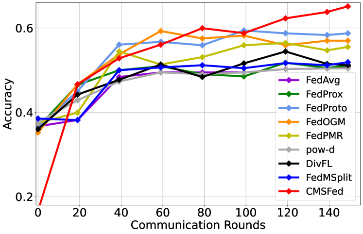
(a) CREMA-D

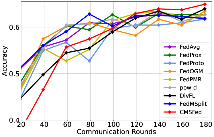
(b) AVE

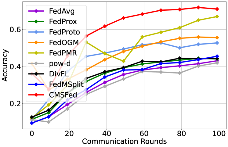
(c) CG-MNIST

Figure 3: Test accuracy of CMSFed compared with other baselines on CREMA-D, AVE and CG-MNIST under IID settings. CMSFed converges to more accurate solutions than all baselines in these three datasets.

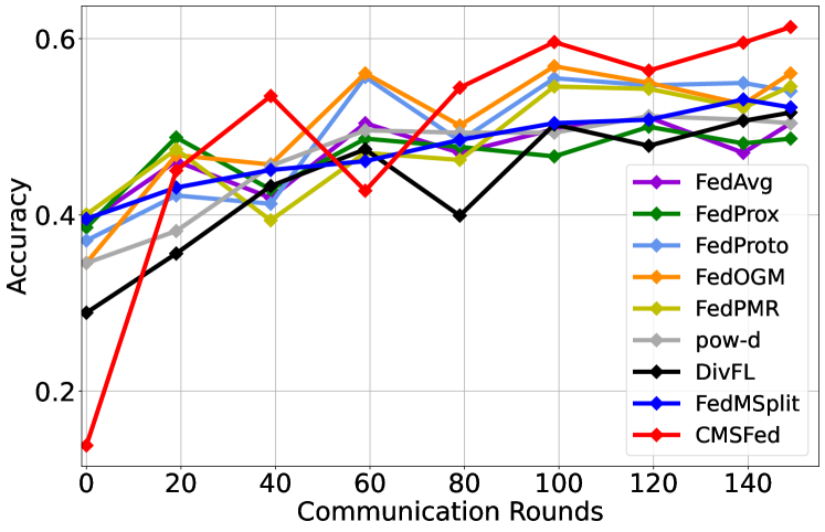
(a) CREMA-D

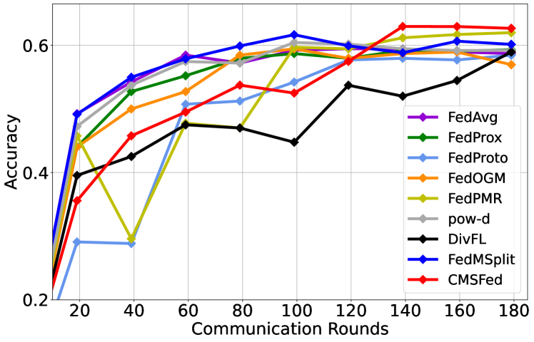
(b) AVE

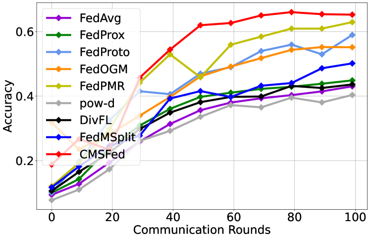
(c) CG-MNIST

Figure 4: Test accuracy of CMSFed compared with other baselines on CREMA-D, AVE and CG-MNIST under non-IID settings. CMSFed still makes remarkable improvement.

Discussion. (1) Mitigating the selection bias in our method are twofold: the PCE loss $\tilde{F}_{k}$ alleviates imbalance at local side and the selected uni-modal clients further promote balanced learning of global model. Meanwhile, the diversity coming from two submodular functions ensures the improvement for the global model. (2) The maximization of $\bar{G}\left(S_{M}\right)$ and $\bar{G}\left(S_{M}\cup S_{I}\right)$ can be viewed as the optimization for multi-modal learning and uni-weak-modal learning respectively. Imbalance ratio is adopted to keep their balance. (3) We assume $I$ is the weak modality above while in practice, we can determine the weak modality before modality selection via the aggregated global imbalance ratio $\rho_{I}$ with $\rho_{I}^{k}$ from all clients. Overall, the pseudo-code of CMSFed is provided in Algorithm 1. (4) Only the gradients, prototypes and $\rho_{I}^{k}$ participate in communication, so there is no privacy issue and similar communication overheads as in traditional FL.

5 Evaluation

5.1 Datasets and baselines

CREMA-D [2] is an audio-visual dataset for emotion recognition task, each video in which consists of both facial and acoustic emotional expressions. There are total 6 categories for emotional states: neutral, happy, sad, fear, disgust and anger. 7,442 clips in total are collected in this dataset. 6,698 samples are randomly chosen as the training set and the rest of 744 samples are the testing set.

AVE [30] is an audio-visual dataset for audio-visual event localization, which consists of 28 event classes and 4,143 10-second video clips with both auditory and visual tracks as well as second-level annotations. All the video clips are collected from YouTube. In our experiments, we aim to construct a labeled multi-modal classification dataset by extracting the frames from event-localized video segments and capturing the audio clips within the same segments. The training and validation splits of the dataset follow [30].

Colored-and-gray MNIST [15] is a synthetic dataset based on MNIST [16], and we denote it as CG-MNIST in this paper. Two kinds of images form a sample pair: a gray-scale image and a monochromatic image. In the training set, there are 60,000 sample pairs, and the monochromatic images are strongly color-correlated with their digit labels, In the validation set, the number of sample pairs is 10,000, while the monochromatic images are weakly color-correlated with their labels. The data synthesis method follows [34]. This dataset is used to prove the method’s effectiveness beyond audio-visual modality.

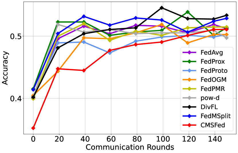
(a) Audio in CREMA-D

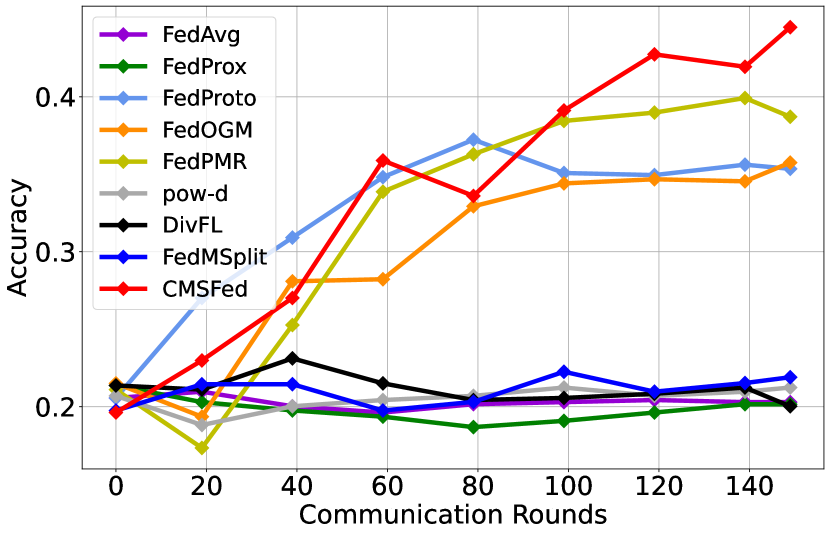
(b) Visual in CREMA-D

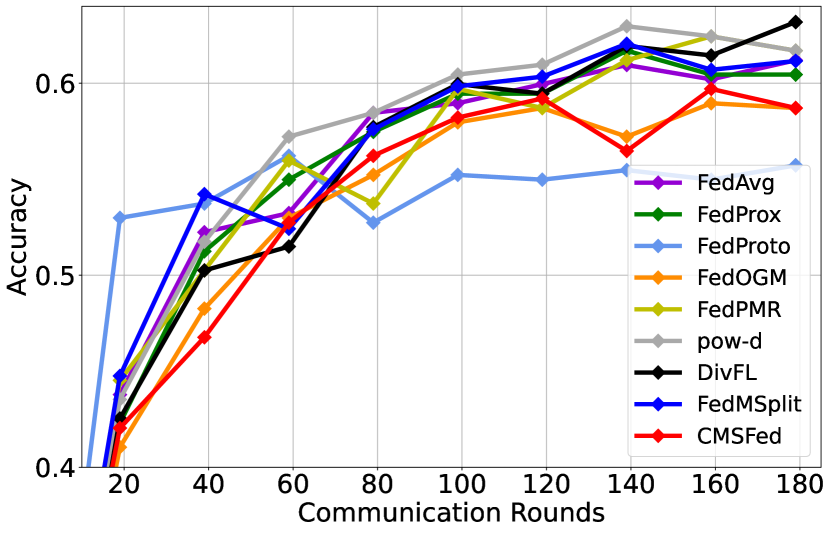
(c) Audio in AVE

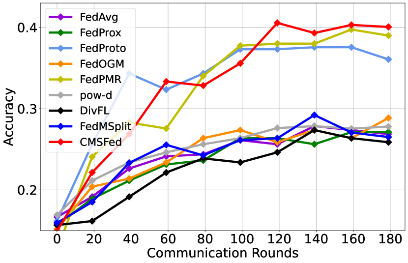
(d) Visual in AVE

Figure 5: The performance of each modality compared with other baselines on CREMA-D and AVE under IID settings. CMSFed achieves comparable audio accuracy and significantly better visual performance simultaneously.

Baselines. We choose eight baselines for comparison from four categories: (1) three uni-modal FL methods designed for statistical heterogeneity are extended to multi-modal scenarios: FedAvg [20], FedProx [18] and FedProto [29]. (2) Integrating OGM-GE [26] and PMR [9], the solutions for modality imbalance, with FedAvg forms two MFL methods: FedOGM and FedPMR. (3) Two client selection method: Power-of-choice (pow-d) [4] and DivFL [1], evolved from its uni-modal version directly. (4) One MFL method, FedMSplit [3], especially designed for modality incongruity. Compared with these baselines, we demonstrate that an elaborate modality selection strategy is essential to realize comprehensive information exploitation in MFL.

5.2 Experimental settings

For CREMA-D and AVE, we use ResNet18 [10] as the backbone for both audio and visual modalities. Audio data is converted to a spectrogram of size 257x299 for CREMA-D and 257×1,004 for AVE. We randomly choose 3 frames and 4 frames to build image training sets for CREMA-D and AVE respectively. For CG-MNIST, we build a neural network with 4 convolution layers and 1 average pool layer as the encoder, following the setting as in [9]. We choose the simple yet effective fusion method, concatenation [25], to build fusion classifier for the three datasets. We set 20 clients for CREMA-D, AVE and 30 clients for CG-MNIST, while 5 clients are selected in each communication round for CREMA-D, AVE and 6 for CG-MNIST. For IID setting, training data is uniformly distributed to clients. For non-IID scenarios, we use Dirichlet distribution [11] $Dir\left(\alpha\right)$ to split data ($\alpha=3$ for CREMA-D and AVE, $\alpha=2$ for CG-MNIST). The optimizer is SGD [28] for all datasets. Learning rate is initialized at 1e-3 or 1e-2 for CEAMA-D and AVE or CG-MNIST and becomes 1e-4 or 1e-3 in the later training stage. The hyper-parameter $\chi$ is set to 1.5-2.5 according to datasets and settings. To complete stochastic greedy algorithm for Eqs. 13 and 14, we use the gradients from the selected clients at current round to update part of the similarity matrix, which is named “no-overheads” in [1]. Except for pow-d, DivFL and CMSFed, other baselines select clients randomly. Each client has two modal data by default if not specified.

5.3 Comparison with baselines

CMSFed effectively improves the performance. As shown in Fig. 3, we report the test accuracy versus the number of communication rounds for three datasets under IID data distributions. We observe that CMSFed can achieve significant improvement compared with all other baselines (by up to 5% on CREMA-D). CMSFed also realizes comparable or even faster convergence speeds in CREMA-D and CG-MNIST. The slow learning at the beginning in AVE is attributed to the need for more effort to explore the information of weak modality. Client sampling here (pow-d and DivFL) cannot fully exploit information for all modalities, making its improvement limited or even worse than FedAvg in CG-MNIST. Although FedOGM and FedPMR accomplish modest improvement because of their ability to alleviate modality imbalance, they are not as good as CMSFed since they do not consider the overall performance of aggregated model. Traditional uni-modal FL methods for statistical heterogeneity (e.g. FedProx) and MFL method for modality incongruity (FedMSplit) only obtain slight improvement. The results for non-IID data distributions are demonstrated in Fig. 4. The overall trends are similar to the results in Fig. 3. These results exhibit the superiority of our method and the importance of meticulously selecting the modalities for training in MFL.

Dataset	CREMA-D		AVE
setting	IID	non-IID	IID	non-IID
FedAvg	50.7	49.8	62.2	59.7
FedAvg-0.8	52.4	50.1	63.4	61.1
FedAvg-0.5	55.7	55.1	60.7	59.4
FedAvg-0.2	61.2	58.1	58.5	58.7
FedAvg+ML	55.8	54.5	62.8	60.7
DivFL+ML	57.1	55.6	63.0	61.1
CMSFed-local	63.7	60.3	63.4	60.1
CMSFed	64.5	61.6	64.7	62.1

Table 1: Ablation study. ‘PCE’ denotes using Eq. 9 for local enhancement. ‘CMSFed-local’ uses local prototypes rather than global prototypes.

CMSFed exploits all modalities comprehensively. To show the effect of our method on modality imbalance, we plot the accuracy curves of each modality on CREMA-D and AVE under IID setting. We can see from Fig. 5 that CMSFed could considerably improve the performance of weak modality (visual) and mitigate the modality-level bias as illustrated in Figs. 5(b) and 5(d). Besides, compared with randomly modal abandoning, which significantly reduces audio performance as illustrated in Fig. 2(b), CMSFed achieves comparable audio performance with other baselines. Since audio modality dominates multi-modal learning in these two datasets, pow-d and DivFL selects clients mainly relying on the loss or gradients from audio, which consequently improve audio performance but no improvement on visual modality. FedMSplit mainly focuses on modality incongruity, which is not an issue here, so there is no notable improvement in both modalities. Although FedProto, FedOGM and FedPMR also alleviate the imbalance, FedProto achieves worse audio behavior and FedOGM and FedPMR only focus on local optimization, resulting in the performance gap between them and our CMSFed on the aggregated model, which further indicates that in MFL, it is important to take both local optimization for each modality and the overall performance for aggregated model into consideration simultaneously.

5.4 Ablation study

Effectiveness of each component. Tab. 1 studies the effect of each CMSFed component. Applying Eq. 9 (FedAvg+PCE) surpasses the vanilla strategy (FedAvg) by a large margin, demonstrating its effectiveness on local enhancement. Comparing CMSFed (64.5% on IID CREMA-D) with ‘DivFL+PCE’ (57.1% on the same setting) also denotes the necessity of balancing different modalities via modality selection. To show the importance of aligning feature spaces of weak modality, we replace the global prototypes with local prototypes (CMSFed-local). Global alignment achieves notable improvement (by up to 2% on non-IID AVE). The performance improvement compared with ‘FedAvg-0.8,0.5,0.2’ exhibits that randomly sampling modalities does not always lead to improvement and further demonstrates the need of meticulously selecting modalities for information exploitation.

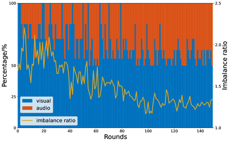
Figure 6: Proportional change of audio and visual respectively and the curve of global imbalance ratio during training on CREMA-D under IID setting.

The relationship between modality selection and imbalance degree. In Eqs. 13 and 14, we use a conflict resolution strategy based on local imbalance ratio to realize balanced modality selection. We visualize the proportions of audio and visual modalities selected in each round and the global imbalance ratio. It is clear from Fig. 6 that audio is the dominant modality (imbalance ratio is always greater than 1) and modality imbalance is gradually alleviated as training progresses (global imbalance ratio shows a downward trend). In addition, the proportion of selected visual modality follows the same trend (larger in the early stage of training and becomes smaller later), implying the rationality of our selection strategy based on imbalance ratio and its effectiveness on mitigating bias.

Effectiveness on modality incongruity scenario. All above experiments assume that each client initially has complete modal data. Here, we build the stimulation of modality incongruity scenario, in which half of the clients have data with two modalities, and the other half only have data in one modality: random audio or visual. The results are shown in Tab. 2 (The results of pow-d is not available because it is not applicable to this scenario). Our CMSFed still makes impressive improvement compared with all other baselines (by up to 3.5% on IID CREMA-D), illustrating the good generalization ability of our method in different scenarios. It is worth mentioning that FedMSplit performs better than before because it is specifically designed for modality incongruity.

Dataset	CREMA-D		AVE
setting	IID	non-IID	IID	non-IID
FedAvg	55.7	55.1	60.7	58.7
FedProx	56.8	56.0	61.2	58.5
FedProto	58.7	57.0	61.3	59.7
FedOGM	58.6	57.4	60.1	58.5
FedPMR	56.4	55.5	61.9	60.3
DivFL	57.4	55.6	61.1	58.6
FedMSplit	58.9	56.9	61.7	60.0
CMSFed	62.4	59.8	63.5	60.9

Table 2: Performance on CREMA-D and AVE with modality incongruity. 50% of clients have all modal data and 50% of clients only retain data with a single modality (audio or visual).

6 Conclusion

In this paper, we analyze traditional client selections in MFL and reveal there exists strong modality-level bias due to the modality imbalance during the training iterations. To address this issue, we propose the client-wise modality selection scheme for MFL (CMSFed) with modality-level gradient decoupling to release the potential of all modalities and maximize the gradient diversities to improve global aggregation. Our method does not introduce additional local training costs and communication overheads compared with previous methods. Extensive experiments on three datasets demonstrate the superiority of our method in performance and applicability under different modal combinations, data distributions and modality incongruity scenarios.

References

- Balakrishnan et al. [2022] Ravikumar Balakrishnan, Tian Li, Tianyi Zhou, Nageen Himayat, Virginia Smith, and Jeff Bilmes. Diverse client selection for federated learning via submodular maximization. In International Conference on Learning Representations, 2022.
- Cao et al. [2014] Houwei Cao, David G Cooper, Michael K Keutmann, Ruben C Gur, Ani Nenkova, and Ragini Verma. Crema-d: Crowd-sourced emotional multimodal actors dataset. IEEE transactions on affective computing, 5(4):377–390, 2014.
- Chen and Zhang [2022] Jiayi Chen and Aidong Zhang. Fedmsplit: Correlation-adaptive federated multi-task learning across multimodal split networks. In Proceedings of the 28th ACM SIGKDD Conference on Knowledge Discovery and Data Mining, pages 87–96, 2022.
- Cho et al. [2020] Yae Jee Cho, Jianyu Wang, and Gauri Joshi. Client selection in federated learning: Convergence analysis and power-of-choice selection strategies. arXiv preprint arXiv:2010.01243, 2020.
- Cornuejols et al. [1977] Gerard Cornuejols, Marshall Fisher, and George L Nemhauser. On the uncapacitated location problem. In Annals of Discrete Mathematics, pages 163–177. Elsevier, 1977.
- Dai et al. [2023] Yutong Dai, Zeyuan Chen, Junnan Li, Shelby Heinecke, Lichao Sun, and Ran Xu. Tackling data heterogeneity in federated learning with class prototypes. In Proceedings of the AAAI Conference on Artificial Intelligence, pages 7314–7322, 2023.
- Deng et al. [2021] Yongheng Deng, Feng Lyu, Ju Ren, Huaqing Wu, Yuezhi Zhou, Yaoxue Zhang, and Xuemin Shen. Auction: Automated and quality-aware client selection framework for efficient federated learning. IEEE Transactions on Parallel and Distributed Systems, 33(8):1996–2009, 2021.
- Duan et al. [2023] Jian-hui Duan, Wenzhong Li, Derun Zou, Ruichen Li, and Sanglu Lu. Federated learning with data-agnostic distribution fusion. In Proceedings of the IEEE/CVF Conference on Computer Vision and Pattern Recognition, pages 8074–8083, 2023.
- Fan et al. [2023] Yunfeng Fan, Wenchao Xu, Haozhao Wang, Junxiao Wang, and Song Guo. Pmr: Prototypical modal rebalance for multimodal learning. In Proceedings of the IEEE/CVF Conference on Computer Vision and Pattern Recognition, pages 20029–20038, 2023.
- He et al. [2016] Kaiming He, Xiangyu Zhang, Shaoqing Ren, and Jian Sun. Deep residual learning for image recognition. In Proceedings of the IEEE conference on computer vision and pattern recognition, pages 770–778, 2016.
- Hsu et al. [2019] Tzu-Ming Harry Hsu, Hang Qi, and Matthew Brown. Measuring the effects of non-identical data distribution for federated visual classification. arXiv preprint arXiv:1909.06335, 2019.
- Huang et al. [2022] Yu Huang, Junyang Lin, Chang Zhou, Hongxia Yang, and Longbo Huang. Modality competition: What makes joint training of multi-modal network fail in deep learning?(provably). In International Conference on Machine Learning, pages 9226–9259. PMLR, 2022.
- Imteaj et al. [2021] Ahmed Imteaj, Urmish Thakker, Shiqiang Wang, Jian Li, and M Hadi Amini. A survey on federated learning for resource-constrained iot devices. IEEE Internet of Things Journal, 9(1):1–24, 2021.
- Karimireddy et al. [2020] Sai Praneeth Karimireddy, Satyen Kale, Mehryar Mohri, Sashank Reddi, Sebastian Stich, and Ananda Theertha Suresh. Scaffold: Stochastic controlled averaging for federated learning. In International conference on machine learning, pages 5132–5143. PMLR, 2020.
- Kim et al. [2019] Byungju Kim, Hyunwoo Kim, Kyungsu Kim, Sungjin Kim, and Junmo Kim. Learning not to learn: Training deep neural networks with biased data. In Proceedings of the IEEE/CVF conference on computer vision and pattern recognition, pages 9012–9020, 2019.
- LeCun et al. [1998] Yann LeCun, Léon Bottou, Yoshua Bengio, and Patrick Haffner. Gradient-based learning applied to document recognition. Proceedings of the IEEE, 86(11):2278–2324, 1998.
- Li et al. [2020a] Tian Li, Anit Kumar Sahu, Ameet Talwalkar, and Virginia Smith. Federated learning: Challenges, methods, and future directions. IEEE signal processing magazine, 37(3):50–60, 2020a.
- Li et al. [2020b] Tian Li, Anit Kumar Sahu, Manzil Zaheer, Maziar Sanjabi, Ameet Talwalkar, and Virginia Smith. Federated optimization in heterogeneous networks. Proceedings of Machine learning and systems, 2:429–450, 2020b.
- Li et al. [2019] Xiang Li, Kaixuan Huang, Wenhao Yang, Shusen Wang, and Zhihua Zhang. On the convergence of fedavg on non-iid data. arXiv preprint arXiv:1907.02189, 2019.
- McMahan et al. [2017] Brendan McMahan, Eider Moore, Daniel Ramage, Seth Hampson, and Blaise Aguera y Arcas. Communication-efficient learning of deep networks from decentralized data. In Artificial intelligence and statistics, pages 1273–1282. PMLR, 2017.
- Mirzasoleiman et al. [2015] Baharan Mirzasoleiman, Ashwinkumar Badanidiyuru, Amin Karbasi, Jan Vondrák, and Andreas Krause. Lazier than lazy greedy. In Proceedings of the AAAI Conference on Artificial Intelligence, 2015.
- Nemhauser et al. [1978] George L Nemhauser, Laurence A Wolsey, and Marshall L Fisher. An analysis of approximations for maximizing submodular set functions—i. Mathematical programming, 14:265–294, 1978.
- Niknam et al. [2020] Solmaz Niknam, Harpreet S Dhillon, and Jeffrey H Reed. Federated learning for wireless communications: Motivation, opportunities, and challenges. IEEE Communications Magazine, 58(6):46–51, 2020.
- Nishio and Yonetani [2019] Takayuki Nishio and Ryo Yonetani. Client selection for federated learning with heterogeneous resources in mobile edge. In ICC 2019-2019 IEEE international conference on communications (ICC), pages 1–7. IEEE, 2019.
- Owens and Efros [2018] Andrew Owens and Alexei A Efros. Audio-visual scene analysis with self-supervised multisensory features. In Proceedings of the European conference on computer vision (ECCV), pages 631–648, 2018.
- Peng et al. [2022] Xiaokang Peng, Yake Wei, Andong Deng, Dong Wang, and Di Hu. Balanced multimodal learning via on-the-fly gradient modulation. In Proceedings of the IEEE/CVF Conference on Computer Vision and Pattern Recognition, pages 8238–8247, 2022.
- Reisizadeh et al. [2022] Amirhossein Reisizadeh, Isidoros Tziotis, Hamed Hassani, Aryan Mokhtari, and Ramtin Pedarsani. Straggler-resilient federated learning: Leveraging the interplay between statistical accuracy and system heterogeneity. IEEE Journal on Selected Areas in Information Theory, 3(2):197–205, 2022.
- Robbins and Monro [1951] Herbert Robbins and Sutton Monro. A stochastic approximation method. The annals of mathematical statistics, pages 400–407, 1951.
- Tan et al. [2022] Yue Tan, Guodong Long, Lu Liu, Tianyi Zhou, Qinghua Lu, Jing Jiang, and Chengqi Zhang. Fedproto: Federated prototype learning across heterogeneous clients. In Proceedings of the AAAI Conference on Artificial Intelligence, pages 8432–8440, 2022.
- Tian et al. [2018] Yapeng Tian, Jing Shi, Bochen Li, Zhiyao Duan, and Chenliang Xu. Audio-visual event localization in unconstrained videos. In Proceedings of the European conference on computer vision (ECCV), pages 247–263, 2018.
- Wang et al. [2021] Haozhao Wang, Zhihao Qu, Song Guo, Ningqi Wang, Ruixuan Li, and Weihua Zhuang. Losp: Overlap synchronization parallel with local compensation for fast distributed training. IEEE Journal on Selected Areas in Communications, 39(8):2541–2557, 2021.
- Wang et al. [2023] Haozhao Wang, Yichen Li, Wenchao Xu, Ruixuan Li, Yufeng Zhan, and Zhigang Zeng. Dafkd: Domain-aware federated knowledge distillation. In Proceedings of the IEEE/CVF Conference on Computer Vision and Pattern Recognition, pages 20412–20421, 2023.
- Wang et al. [2020] Weiyao Wang, Du Tran, and Matt Feiszli. What makes training multi-modal classification networks hard? In Proceedings of the IEEE/CVF conference on computer vision and pattern recognition, pages 12695–12705, 2020.
- Wu et al. [2022] Nan Wu, Stanislaw Jastrzebski, Kyunghyun Cho, and Krzysztof J Geras. Characterizing and overcoming the greedy nature of learning in multi-modal deep neural networks. In International Conference on Machine Learning, pages 24043–24055. PMLR, 2022.
- Xiong et al. [2022] Baochen Xiong, Xiaoshan Yang, Fan Qi, and Changsheng Xu. A unified framework for multi-modal federated learning. Neurocomputing, 480:110–118, 2022.
- Xu and Wang [2020] Jie Xu and Heqiang Wang. Client selection and bandwidth allocation in wireless federated learning networks: A long-term perspective. IEEE Transactions on Wireless Communications, 20(2):1188–1200, 2020.
- Yu et al. [2023] Qiying Yu, Yang Liu, Yimu Wang, Ke Xu, and Jingjing Liu. Multimodal federated learning via contrastive representation ensemble. arXiv preprint arXiv:2302.08888, 2023.
- Zhao et al. [2022] Yuchen Zhao, Payam Barnaghi, and Hamed Haddadi. Multimodal federated learning on iot data. In 2022 IEEE/ACM Seventh International Conference on Internet-of-Things Design and Implementation (IoTDI), pages 43–54. IEEE, 2022.