Controllable Safety-Critical Closed-loop Traffic Simulation via Guided Diffusion

Abstract

Evaluating the performance of autonomous vehicle planning algorithms necessitates simulating long-tail traffic scenarios. Traditional methods for generating safety-critical scenarios often fall short in realism and controllability. Furthermore, these techniques generally neglect the dynamics of agent interactions. To mitigate these limitations, we introduce a novel closed-loop simulation framework rooted in guided diffusion models. Our approach yields two distinct advantages: 1) the generation of realistic long-tail scenarios that closely emulate real-world conditions, and 2) enhanced controllability, enabling more comprehensive and interactive evaluations. We achieve this through novel guidance objectives that enhance road progress while lowering collision and off-road rates. We develop a novel approach to simulate safety-critical scenarios through an adversarial term in the denoising process, which allows the adversarial agent to challenge a planner with plausible maneuvers, while all agents in the scene exhibit reactive and realistic behaviors. We validate our framework empirically using the NuScenes dataset, demonstrating improvements in both realism and controllability. These findings affirm that guided diffusion models provide a robust and versatile foundation for safety-critical, interactive traffic simulation, extending their utility across the broader landscape of autonomous driving. For additional resources and demonstrations, visit our project page at https://safe-sim.github.io.

1 Introduction

A key safety feature of autonomous vehicles (AVs) is their ability to navigate near-collision events in real-world scenarios. However, these events rarely occur on roads and testing AVs in such high-risk situations on public roads is unsafe. Therefore, simulation is indispensable in the development and assessment of AVs, providing a safe and reliable means to study their safety and dependability. A key aspect in the design of simulation is the behavior modeling of other road users since AVs must learn to interact with them safely.

A common method of safety-critical testing of AVs involves manually designing scenarios that could potentially lead to failures, such as collisions. While this approach allows for targeted testing, it is inherently limited in scalability and lacks the comprehensiveness required for thorough evaluation. Some recent works focus on automatically generating challenging scenarios that cause planners to fail, but their emphasis has been mostly on static scenario generation rather than dynamic, closed-loop simulations. This results in a critical gap: the behavior of other agents often does not adapt or respond to the planner’s actions, which is essential for a comprehensive safety evaluation. Furthermore, the results from these simulations often lack controllability, typically producing only a single adversarial outcome per scenario without the flexibility to explore a range of conditions and responses.

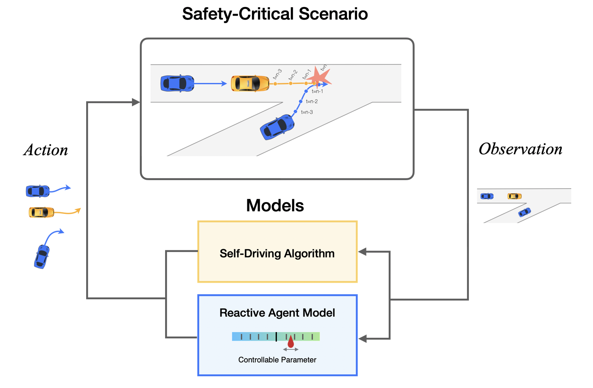
Figure 1: Overview of Controllable Safety-Critical Closed-Loop Simulation Framework. This framework involves evaluating a planner within scenarios featuring multiple reactive agents. These agents possess two distinct qualities: they are trained using real-world driving data, ensuring realistic behavior, and their actions are controllable. Such a setup facilitates the generation of various realistic, interactive, and safety-critical scenarios, providing a thorough evaluation of the planner’s capabilities.

In this work, we introduce a closed-loop simulation framework for generating safety-critical scenarios, with a particular emphasis on controllability and realism for the behavior of agents, which allows simulations over a long-horizon as needed to evaluate AV planning algorithms (Fig. 1). Our approach builds upon recent developments in controllable diffusion models [1, 2, 3]. Specifically, we adopt test-time guidance to direct the denoising phase of the diffusion process, using the gradients from differentiable objectives to enhance scenario generation. Different from prior works, we formulate guidance objectives and strategies that are better for long-term scene-consistent simulation. Additionally, we advance adversarial scenario generation by introducing closed-loop and controllable methods that do not rely on traditional adversarial optimization. Our balanced integration of adversarial objectives with regularization during the guidance phase allows better control over the conditions of the generated scenarios, ensuring both their realism and relevance to safety-critical testing.

In our study, we use the nuScenes dataset [4] to evaluate the efficacy of our method in generating safety-critical closed-loop simulations. Our results demonstrate a marked improvement in controllability and realism of scenarios compared to traditional adversarial scenario generation methods. Furthermore, we showcase the advantage of our proposed guidance strategy in maintaining scene consistency, characterized by the absence of collisions and off-road incidents, while also achieving high progress on the road. These attributes make our approach particularly well-suited for the closed-loop simulation of AVs, providing a more reliable and comprehensive framework for safety evaluation.

2 Related Work

2.1 Traffic Behavior Simulation

Traffic simulation can broadly be categorized into two main groups: heuristic-based and learning-based methods. In heuristic-based method, agents are controlled by human-specified rules, such as the Intelligent Driver Model (IDM) [5] to follow a leading vehicle while maintaining a safe following distance. However, these methods have modeling capacity issue and may not reflect the real traffic distribution, a large domain gap limits its usage for planning evaluation. To close the gap, data-driven approaches imitate real-world behavior by learning from real driving datasets [6]. Such approaches include TrafficSim [7], which performs scene-level traffic simulation via trained variational autoencoder, and BITS [8], which considers high-level goal inference and low-level driving behavior imitation to simulate the driving behavior. However, little work has focused on behavior simulation for generating safety-critical, long-tail scenarios.

Recently, diffusion models [9, 10, 11] have shown significant promise for synthetic image generation. One of the key advantages of diffusion models is controllability, which can take the form of classifier [12], classifier-free [13], and reconstruction [14] guidance. More recently, controllable diffusion models have been employed for planning and traffic simulation [2, 3] via guidance. We adopt trajectory diffusion models to generate safety-critical realistic traffic simulations.

2.2 Safety-Critical Traffic Scenario Geneartion

Safety-critical traffic generation plays a crucial role in training and evaluating AV systems, enhancing their capability to navigate diverse real-world scenarios and enhancing robustness. Gradient-based methods that leverage back-propagation to create safety-critical scenarios have been proposed to evaluate AV prediction and planning models[15][16]. Hanselman et al. use kinematic gradients to modify vehicle trajectories, with the goal of improving the robustness of imitation learning planners [15]. Cao et al. have developed a model with differentiable dynamics, enabling the generation of realistic adversarial trajectories for trajectory prediction models through backpropagation techniques [16]. Black-box optimization approaches include perturbing actions based on kinematic bicycle models [17] and using Bayesian Optimization to create adversarial self-driving scenarios that escalate collision risks with simulated entities [18]. Zhang et al.target trajectory prediction models via white- and black-box attacks that adversarially perturb real driving trajectories [19]

The field has recently seen advancements in data-driven methods for safety-critical scenario generation [20][21][22]. For instance, Xu et al. introduce a diffusion-based approach in CARLA applying various adversarial optimization objectives to guide the diffusion process for safety-critical scenario generation [21]. Rempe et al. proposed STRIVE to utilize gradient-based adversarial optimization on the latent space, constrained by a graph-based CVAE traffic motion model, to generate realistic safety-critical scenarios for rule-based planners [22]. However, a common limitation in these approaches is the absence of closed-loop interaction, essential for accurately simulating interactive real-world driving.

3 Method

3.1 Problem Formulation

We consider a simulated interactive traffic scenario (shown in  Fig. 1) consisting of $N$ agents; one is the ego vehicle controlled by the planner $\pi$, while the remaining $N-1$ are reactive agents modeled by a function $g$. Our objective is to create a safety-critical closed-loop simulation where reactive agents demonstrate realistic, controllable behavior. This setup allows for the identification of possible failures in the planner, such as collision events.

In the traffic scenario, at any given timestep $t$, the states of the $N$ vehicles are represented as $\mathbf{s}_{t}=[\mathbf{s}^{1}_{t},\ldots,\mathbf{s}^{N}_{t}]$, where $\mathbf{s}^{i}_{t}=(x^{i}_{t},y^{i}_{t},v^{i}_{t},\theta^{i}_{t})$ indicates the 2D position, speed, and yaw of vehicle $i$. The corresponding actions for each vehicle are $\mathbf{a}_{t}=[\mathbf{a}^{1}_{t},\ldots,\mathbf{a}^{N}_{t}]$, with $\mathbf{a}^{i}_{t}=(\dot{v}^{i}_{t},\dot{\theta}^{i}_{t})$ representing the acceleration and yaw rate. To predict the state at the next timestep $t+1$, a transition function $f$ is used, which computes $\mathbf{s}_{t+1}=f(\mathbf{s}_{t},\mathbf{a}_{t})$ based on current state and action. We adopt unicycle dynamics as the transition function.

Each agent’s decision context is $\mathbf{c}^{i}_{t}$, which includes the agent-centric map $I^{i}$ and the $T_{\text{hist}}$ historical states of neighboring vehicles from time $t-T_{\text{hist}}$ to $t$, defined as $\mathbf{s}_{t-T_{\text{hist}}:t}=\{\mathbf{s}_{t-T_{\text{hist}}},\ldots,\mathbf{s}_{t}\}$. In closed-loop traffic simulation, each agent continuously generates and updates its trajectory based on the current decision context $\mathbf{c}^{i}_{t}$. After generating a trajectory, the simulation executes the first few steps of the planned actions before updating $\mathbf{c}^{i}_{t}$ and re-planning.

Planner $\pi$. The planner $\pi$ determines the ego vehicle’s future trajectory over a time horizon $t$ to $t+T$. The planned state sequence is denoted by $s^{1}_{t:t+T}=\pi(\mathbf{c}^{1}_{t})$, where $\pi(\mathbf{c}^{1}_{t})$ processes the historical states and map data within $\mathbf{c}^{1}_{t}$ to plan future states based on the current scene context.

Reactive Agents $g$. The reactive agent model $g$, parameterized by $\theta$, is designed to simulate the behavior of the $N-1$ non-ego vehicles, represented by the set $\{s^{i}_{t:t+T}\}_{i=2}^{N}$. Each vehicle’s state sequence, $s^{i}_{t:t+T}$, is generated by $g_{\theta}(\mathbf{c}^{i}_{t},\psi_{i})$, which incorporates the decision context $\mathbf{c}^{i}_{t}$ and a set of control parameters $\psi_{i}$ unique to each agent. These parameters $\psi_{i}$ enable the fine-tuning of individual behaviors within the simulation. In our approach, we train the model $g$ on real-world driving data to ensure the trajectories it produces are not only controllable, supporting the generation of various safety-critical scenarios, but also realistic.

Adversarial Agent in Safety-Critical Scenarios. The adversarial agent, formulated within the reactive agent model $g$, is governed by an adversarial term designed (detailed in Sec. 3.3) to be both controllable and adversarial to the planner $\pi$. This setup allows the adversarial agent to pose direct challenges to $\pi$, testing its resilience in complex scenarios. Concurrently, the other non-adversarial agents, also controlled by $g$ with varying parameters, emulate authentic, reactive behaviors, thus enriching the simulation scenario with realistic and diverse traffic conditions. The dual role of the adversarial agent and non-adversarial agents ensures that while it challenges $\pi$, the overall simulation environment plausibly represents real-world driving conditions.

3.2 Controllable Reactive Agents

For closed-loop traffic simulation, the reactive agents should be 1) controllable, and 2) realistic. With recent advances in controllable diffusion models [1, 2, 3], we adopt trajectory diffusion models to generate realistic simulations. We define the model’s operational trajectory as $\tau$, which comprises both action and state sequences: $\tau:=[\tau_{a},\tau_{s}]$. Specifically, $\tau_{a}:=[a_{0},\ldots,a_{T-1}]$ represents the sequence of actions, while $\tau_{s}:=[s_{1},\ldots,s_{T}]$ denotes the corresponding sequence of states. Following the approach described in [2], our model predicts the action sequence $\tau_{a}$, and the state sequence $\tau_{s}$ can be derived starting from the initial state $s_{0}$ and dynamic model $f$. We provide background on trajectory diffusion for completeness, before describing our contributions for controllable guidance.

Trajectory Diffusion. A diffusion model generates a trajectory by reversing a process that incrementally adds noise. Starting with an actual trajectory $\tau_{0}$ sampled from the data distribution $q(\tau_{0})$, a sequence of increasingly noisy trajectories $(\tau_{1},\tau_{2},\ldots,\tau_{K})$ is produced via a forward noising process. Each trajectory $\tau_{k}$ at step $k$ is generated by adding Gaussian noise parameterized by a predefined variance schedule $\beta_{k}$ [23]:

$$q(\tau_{1:K}|\tau_{0}):=\prod_{k=1}^{K}q(\tau_{k}|\tau_{k-1}),$$ (1)

$$q(\tau_{k}|\tau_{k-1}):=\mathcal{N}(\tau_{k};\sqrt{1-\beta_{k}}\tau_{k-1},\beta_{k}\mathbf{I}).$$ (2)

The noising process gradually obscures the data, where the final noisy version $q(\tau_{K})$ approaches $\mathcal{N}(\tau_{K};\mathbf{0},\mathbf{I})$. The trajectory generation process is then achieved by learning the reverse of this noising process. Given a noisy trajectory $\tau_{K}$, the model learns to denoise it back to $\tau_{0}$ through a sequence of reverse steps. Each reverse step is modeled as:

$$p_{\theta}(\tau_{k-1}|\tau_{k},\mathbf{c}):=\mathcal{N}(\tau_{k-1};\mu_{\theta}(\tau_{k},k,\mathbf{c}),\Sigma_{k}),$$ (3)

where $\theta$ are learned functions that predict the mean of the reverse step, and $\Sigma_{k}$ is a fixed schedule. By iteratively applying the reverse process, the model learns a trajectory distribution, effectively generating a plausible future trajectory from a noisy start.

During the trajectory prediction phase, the model estimates the final clean trajectory denoted by $\hat{\tau}_{0}$. This estimated trajectory is used to compute the reverse process mean $\mu$ as described in [24]. For more details, see Section 10.3.

The training objective is to minimize the expected difference between the true initial trajectory and the one estimated by the model, formalized by the loss function [2][24]:

$$\mathcal{L}=\mathbb{E}_{\epsilon,k,\tau_{0},c}\left[\|\tau_{0}-\hat{\tau}_{0}\|^{2}\right]$$ (4)

where $\tau_{0}$ and $\mathbf{c}$ are sampled from the training dataset, $k\sim\mathcal{U}\{1,2,\ldots,K\}$ is the timestep index sampled uniformly at random, and $\epsilon\sim\mathcal{N}(0,\mathbf{I})$ is Gaussian noise used to perturb $\tau_{0}$ to produce the noised trajectory $\tau_{k}$.

3.2.1 Controllability: Guidance on Diffusion Model

The diffusion model, once trained on realistic trajectory data, inherently reflects the behavioral patterns present in its training distribution. However, to effectively simulate and analyze safety-critical scenarios, there is a crucial need for a mechanism that allows for the controlled manipulation of agent behaviors [1, 2]. This is particularly important for generating adversarial behaviors and ensuring long-term scene consistency in simulations.

Our approach specifically introduces guidance to the sampled trajectories at each denoising step, aligning them with predefined objectives $J(\tau)$. The concept of guidance involves using the gradient of $J$ to subtly perturb the predicted mean of the model at each denoising step. This process enables the generation of trajectories that not only reflect realistic behavior but also cater to specific simulation needs, such as adversarial testing and maintaining scene consistency over extended periods.

3.2.2 Clean Guidance for Traffic Simulation

Clean guidance is essential in trajectory simulation to manage the challenges of noisy data, which can lead to errors and instability [3, 25]. This method focuses on refining the model’s clean prediction $\hat{\tau}_{0}$, rather than trying to correct the noisy data directly. Given that the denoising steps involve handling noisy trajectory data, which could lead to numerical instability, the guidance operates on the model’s clean prediction $\hat{\tau}_{0}$ instead (shown in Fig. 2). We adjust the clean prediction using:

$$\tilde{\tau}_{0}=\hat{\tau}_{0}-\alpha\Sigma_{k}\nabla_{\tau_{k}}J(\hat{\tau}_{0}).$$ (5)

This strategy improves guidance robustness, yielding smoother, more stable trajectories without the usual numerical issues from noisy data.

The effectiveness of clean guidance is evident from our experimental results. Without clean guidance, we notice significant problems like very low road progress in simulation, which also has the side-effect of incorrectly conveying low collision and off-road rates. Detailed results and further discussion on this topic can be found in Sec. 4.6.

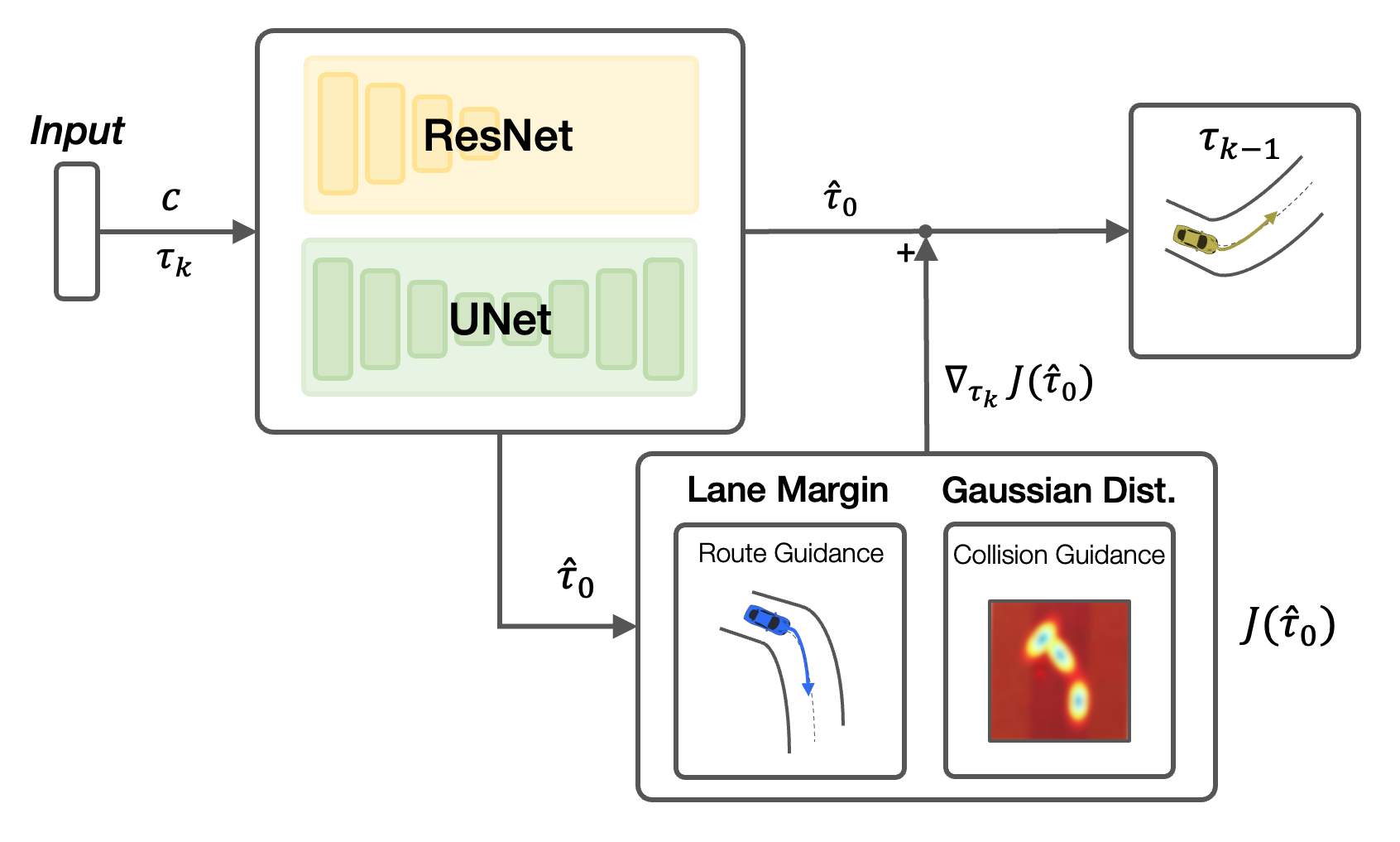
Figure 2: Illustration of Clean Guidance in Traffic Simulation. This technique refines the model’s clean prediction $\hat{\tau}_{0}$ using our proposed guidance functions: Route guidance and Gaussian collision guidance, which enhances trajectory stability and realism by avoiding the pitfalls of noisy data.

3.2.3 Novel Guidances for Controllable Diffusion

In closed-loop traffic simulation, ensuring long-horizon stability is crucial [26]. Our experimental observations, as detailed in Sec. 4, indicate that without proper guidance, diffusion models may result in the ego vehicle deviating from the drivable area or engaging in collisions. To mitigate these issues and promote long-duration realistic simulation fidelity, we introduce two novel guidance functions: route-based and Gaussian collision guidance. These functions effectively constrain the vehicle’s trajectory, ensuring adherence to traffic routes and safe distances from other participants in the simulation, as discussed in Sec. 4.6.

Route Guidance. Given an agent’s trajectory $\tau$ and the corresponding route $r$, we compute the normal distance of each point $\tau_{t}$ on the trajectory to the route at each timestep. We then penalize deviations from the route that exceed a predefined margin $d$. This process is captured by the following route guidance cost function:

$$J_{\text{route}}(\tau,r)=\sum_{t=1}^{T}\max(0,|d_{n}(\tau_{t},r)-d_{m}|),$$ (6)

where $d_{n}(\tau_{n},r)$ denotes the normal distance from the point $\tau_{t}$ on the trajectory to the nearest point on the route $r$ at timestep $t$, and $d_{m}$ represents the acceptable deviation margin from the route. In contrast to the off-road loss in prior studies [2], our proposed route guidance system offers a stronger indication of each agent’s long-term destination, which contributes to improvement on traffic rules as shown in Sec. 4. One advantage is to simulate various interactions between the route choices of the ego agent and other agents within the simulation [27]. Additionally, its flexibility accommodates diverse behaviors, such as modifying routes to encourage lane-changing among reactive agents.

Gaussian Collision Guidance. Given the trajectories of agents, we calculate the Gaussian distance for each pair of agents $(i,j)$ at each timestep $t$ from $1$ to $T$. The Gaussian distance between the agents takes into account both the tangential ($d_{t}$) and normal ($d_{n}$) components of the projected distances. The aggregated Gaussian distance is:

$$J_{\text{gc}}=\sum_{t=1}^{T}\sum_{i,j}^{N}\exp\left(-\frac{1}{2\sigma^{2}}\left(\lambda\cdot{d_{t}^{ij}}(t)^{2}+{d_{n}^{ij}}(t)^{2}\right)\right)$$ (7)

where $d_{t}^{ij}(t)$ and $d_{n}^{ij}(t)$ represent the tangential and normal distances from agent $j$’s trajectory point at time $t$ to agent $i$’s heading axis, respectively, and $\sigma$ is the standard deviation for these distances. In this formulation, $\lambda$ is a scaling factor applied to the tangential distance $d_{t}^{ij}(t)$. This approach contrasts with the disk approximation method, which primarily penalizes the Euclidean distance between agents. By accounting for both tangential and normal components, the Gaussian collision distance method significantly enhances collision rate, which we discuss in Sec. 4.

Note that the collision guidance is based on different agent interactions. Following the methodology of [2], we extend the denoising process of all agents within a scene into the batch dimension. During inference, to generate $M$ samples, we proceed under the assumption that each sample corresponds to the same $m$-th example of the scene. For the ego vehicle, the future state predictions are derived from a diffusion model identical to the one used for other agents. The collision distance for the ego vehicle is then computed considering these predictions and their interactions with other agents within the scene.

3.3 Safety-Critical Closed-Loop Simulation

A comprehensive testing approach for AVs under safety-critical scenarios must emphasize realism and controllability. The simulation includes an “ego agent” (the AV under test, indexed as agent 1), non-adversarial reactive agents, and an adversarial agent (denoted as agent $a$), shown in Fig. 3. These agents engage in dynamic, closed-loop interactions, contributing to a realistic and controlled environment for evaluating AV performance. As mentioned in  Sec. 3.1, our framework integrates an adversarial term in the denoising process for simulating safety-critical interactions. The loss function for the adversarial agent, $J(\tau)$, consists of an adversarial component $J_{\text{adv}}$ and a regularization $J_{\text{reg}}$. The adversarial component $J_{\text{adv}}$ itself is comprised of a collision term $J_{\text{coll}}$ and a control term $J_{\text{control}}$.

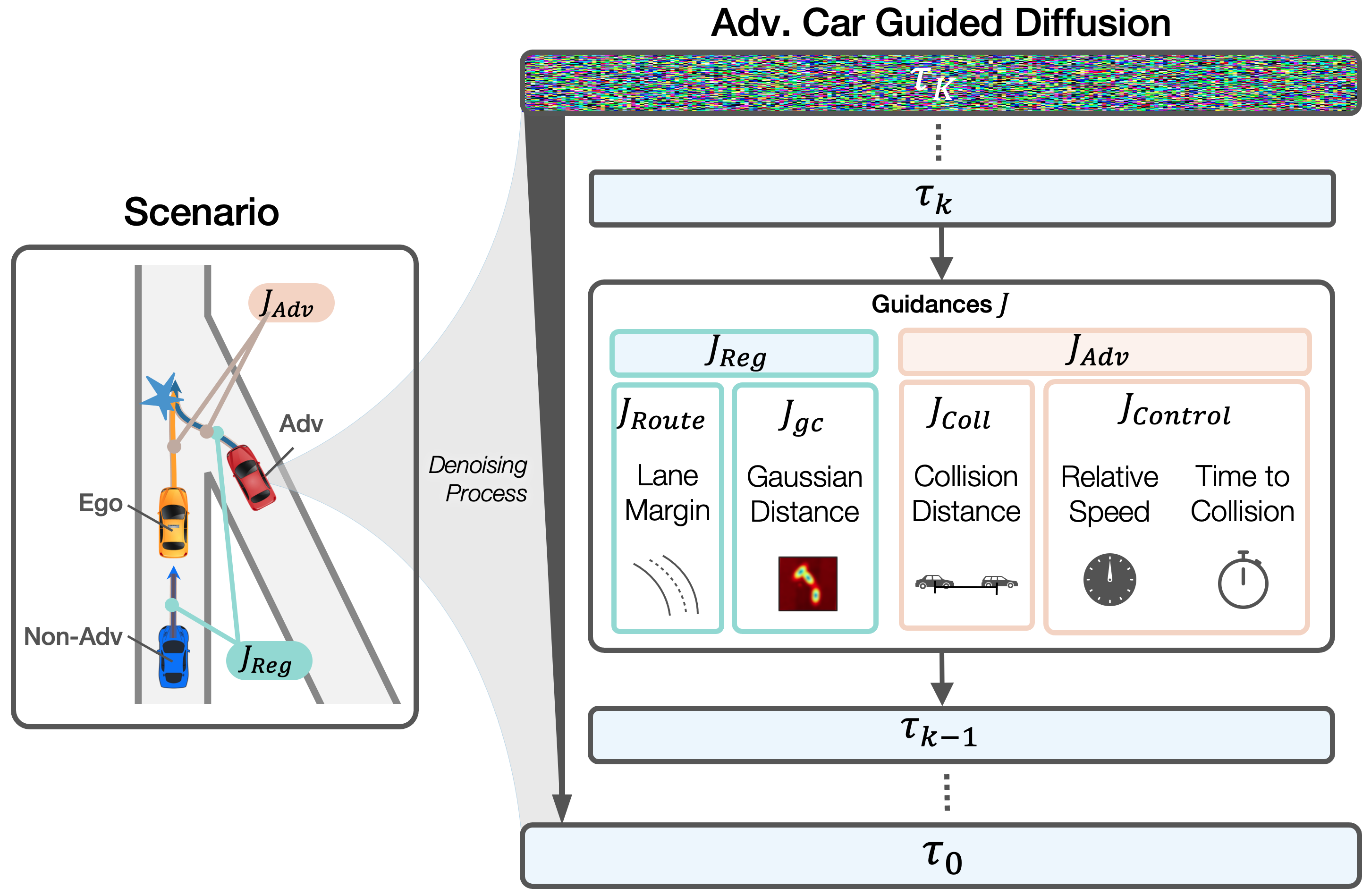
Figure 3: Guided Diffusion Process for the Adversarial Agent. This process optimizes the adversarial agent’s trajectory using the adversarial cost function $J_{\text{adv}}$ in relation to the ego vehicle. Simultaneously, it applies regularization through $J_{\text{reg}}$ for maintaining realism. Within $J_{\text{adv}}$, the $J_{\text{control}}$ component is incorporated to control the adversarial behavior of the agent.

Method	Length	Ego-Adv Coll	Ego-Other Coll	Other Offroad	Adv Offroad	Adv Speed	Realism
	(s)	(%) $\uparrow$	(%) $\uparrow$	(%) $\downarrow$	(%) $\downarrow$	(m/s) $\downarrow$	$\downarrow$
STRIVE	6	36.7	38.2	16.1	25.0	4.01	0.85
Ours	6	25.0	26.5	18.0	11.8	2.04	0.43
Ours	12	38.2	42.7	23.2	8.8	2.63	0.48

Table 1: Comparison between STRIVE [22] and our approach for safety-critical generation for a rule-based planner.. Our framework demonstrates enhanced performance in Ego-Adversary collision rate with reduced adversary’s off-road rate and improved realism

Rel Speed	Ego-Adv Rel	Coll Rate	Realism
Control (m/s)	Speed (m/s)	(%) $\uparrow$	$\downarrow$
-2.0	0.90	0.38	0.83
0.0	1.26	0.38	0.89
2.0	1.94	0.50	0.88
No control	3.94	0.72	0.82

Table 2: Controllability of relative collision speed. This table illustrates the ability of our framework to modulate the relative speed between ego and adversarial agents, influencing collision rates while maintaining realism.

Collision with Planner. We define $J_{\text{coll}}$ to encourage the collision between the adversarial agent and the ego agent, given by:

$$J_{\text{coll}}=-\sum_{t=1}^{T}d(t)-d_{\text{min}},$$ (8)

where $d(t)$ represents the distance at each time step, and $d_{\text{min}}$ is the minimum distance observed between the ego and the adversarial agent in the planning horizon $T$.

Controlling the Adversarial Collision Behavior. We propose that a guidance $J_{\text{control}}$ may control different behaviors of the adversarial agent that causes the collision. In this work, we choose to control the relative speed $J_{v}$ between the ego and adversary at each time step ($v^{1}_{t}$ and $v^{a}_{t}$) and the time-to-collision (TTC) cost $J_{\text{ttc}}$ [28] to control the safety criticality of potential collisions, with the latter given by:

$$J_{\text{ttc}}=\sum_{t=1}^{T}-\exp\left(-\frac{\tilde{t}_{\text{col}(t)}^{2}}{2\lambda_{t}}-\frac{\tilde{d}_{\text{col}(t)}^{2}}{2\lambda_{d}}\right),$$ (9)

where $\tilde{t}_{\text{col}(t)}$ is the time to collision at time $t$, $\tilde{d}_{\text{col}(t)}$ is the distance to collision and $\lambda_{t}$ and $\lambda_{d}$ are bandwidth parameters for time and distance. This formula uses a constant velocity assumption. Intuitively, The time-to-collision cost favors scenarios with high relative speeds and challenging collision angles for the ego vehicle to avoid. For a detailed explanation of $J_{\text{ttc}}$, see  Sec. 9.

Regularization. The regularization term, $J_{\text{reg}}$, plays a crucial role in balancing the adversarial agent’s behavior within our simulation framework. $J_{\text{route}}$ ensures that the adversarial agent adheres to its predefined paths, contributing to the overall plausibility of the traffic scenario. Meanwhile, $J_{\text{gc}}$, applied to the adversarial agent’s interactions with non-adversarial agents, ensures that the behavior of the adversarial agent realistically avoids collisions with these agents, in line with standard traffic scenarios. This approach ensures that the adversarial agent poses a realistic challenge to the ego agent of the simulation environment.

Approach to Adversarial Simulation. Our approach begins by setting up scenarios based on actual traffic logs. We emphasize three key benefits of our safety-critical simulation approach:

1. Control over safety-critical scenarios is a significant improvement, allowing behavior modification through $J_{\text{adv}}$.

2. Unlike previous methods, our framework only nudges agent behavior towards aggressiveness without globally altering the scenario dynamics. This selective approach ensures realistic interactions.

3. All agents interact in a closed-loop simulation, providing a more comprehensive assessment than methods where only the planner responds to other agents. This captures the mutual influence of agents’ actions, which is often overlooked in previous works.

Finally, we note that our simulation can run for extended periods, not constrained by the traffic model duration limits seen in prior works [22]. This allows for thorough testing of autonomous vehicles over longer scenarios.

4 Experiments

We validate the efficacy of our proposed framework via experiments with real-world driving data. Our results demonstrate that the framework can generate controllable and realistic safety-critical scenarios, essential for comprehensive autonomous vehicle (AV) testing. Additionally, we highlight the effectiveness of our newly introduced guidance strategies within the diffusion model, which contribute to the stability and realism of the simulation environment.

4.1 Dataset

We conduct our experiments on nuScenes [6], a large-scale real-world driving dataset consisting of 5.5 hours of driving data from two cities. We train the model on scenes from the train split and evaluate it on the scenes from the validation split. We focus on vehicle-to-vehicle interactions.

4.2 Implementation Details

Planner. Our experiments utilize a rule-based planner, as implemented in [22]. This planner operates on the lane graph and employs the constant velocity model to predict future trajectories of non-ego vehicles. It generates multiple trajectory candidates, selecting the one least likely to result in a collision.

Diffusion Model. We follow the architecture described in [2]. We represent the context using an agent-centric map and past trajectories on a rasterized map. The traffic scene is encoded using a ResNet structure [29], while the input trajectory is processed through a series of 1D temporal convolution blocks in an UNet-like architecture, as detailed in [1]. The model uses $K=100$ diffusion steps. During the inference phase, we generate a sample of potential future trajectories for each reactive agent in a given scene. From these, we select the trajectory that yields the lowest guidance cost. This process is referred to as filtering.

Closed-loop Simulation. The simulation framework for our experiments is built upon an open-source traffic behavior framework [26]. Within this framework, both the planner and reactive agents update their plans at a frequency of 2Hz. We randomly select an adversarial agent whose lane proximity to the ego vehicle falls within a predefined threshold.

4.3 Evaluation Metrics

Our goal is to validate that the proposed method can generate safety-critical scenarios that are both realistic and controllable. For realism assessment, in accordance with [2], we compare statistical data between simulated trajectories and actual ground trajectories. This involves calculating the Wasserstein distance between their driving profiles’ normalized histograms, focusing on the mean of mean values for three properties: longitudinal acceleration, latitudinal acceleration, and jerk. To evaluate controllability, we measure metrics related to parameters we can control, specifically relative speed and time-to-collision cost between the ego and adversarial agents.

For a more nuanced understanding of realism, we analyze the collision rate – the average fractions of agents colliding, and the offroad rate – the percentage of reactive agents going off-road, both of which are considered failure rates [26]. We also include the road progress to evaluate agents’ distance traveled along their designated lane centerlines, and wrong direction rate. All metrics are averaged across scenarios. For detailed definitions and metrics, see Sec. 9.

TTC Cost weight	TTC Cost	TTC	Coll Speed	Coll Angle	Coll Rate	Realism
		(s)	(m/s)	(deg)	(%) $\uparrow$	$\downarrow$
0.0	0.24	11.39	2.45	12.76	0.53	0.83
1.0	0.29	6.83	2.30	6.47	0.50	0.89
2.0	0.36	3.03	3.78	1.00	0.7	0.88

Table 3: Evaluating Time to Collision (TTC) Control. The table shows the impact of different TTC Cost weights on collision scenarios. Increasing the TTC Cost weight results in a decrease in time to collision and an increase in collision rate, suggesting a heightened challenge for the ego vehicle in avoiding collisions.

Method	Coll Rate	Off Road	Failure Rate	Wrong Direction	Realism
	(%) $\downarrow$	(%) $\downarrow$	(%) $\downarrow$	(%) $\downarrow$	$\downarrow$
CTG no collision	4.0	27.1	27.1	-	0.569
CTG off-road	11.4	34.1	45.5	-	0.569
CTG*	21.84	0.13	21.96	9.31	0.754
Ours	3.49	0.87	4.18	6.54	0.87

Table 4: Comparative Analysis in Closed-Loop Traffic Simulation. While our approach exhibits a slightly higher realism, it significantly outperforms both CTG versions in terms of reduced failure rate and improved wrong direction rate, highlighting the efficacy of our proposed guidance strategies.

Model	Collision (%)	Off-road (%)	Progress (m)	Wrong Direction(%)	Realism
Ours (- $J_{gc}$)	30.82	0.46	48.1	8.72	0.71
Ours (- $J_{route}$)	3.03	3.48	51.2	23.9	1.08
Ours (- clean guide)	5.15	0.32	11.8	4.65	0.55
Ours	4.21	1.15	56.8	9.37	0.96

Table 5: Ablation study on diffusion model guidance functions. Results show the effectiveness of $J_{gc}$ in reducing collision rates, the role of $J_{route}$ in managing wrong-direction incidents, and the impact of clean guidance on improving the progress of reactive agents.

4.4 Safety-Critical Simulation Evaluation

We initiated our evaluation by comparing our method with STRIVE [22], recognized for its proficiency in generating adversarial safety-critical scenarios using a learned traffic model and adversarial optimization in the latent space. Our comparison focused on the collision rates between the ego and adversarial agents (referred to as ”Ego-Adv”), the collision rates involving other (non-adversarial reactive) agents (”Ego-Other”), and the off-road rate for the adversarial agent (”Adv Offroad”). The results are presented in Tab. 1.

Our method excels in realism and control, showcasing higher adversarial collision rates and better realism. Firstly, it demonstrates a higher Ego-Adv collision rate, indicating a more effective generation of safety-critical scenarios. Notably, this is achieved with a significantly lower Adv Offroad rate and better realism.

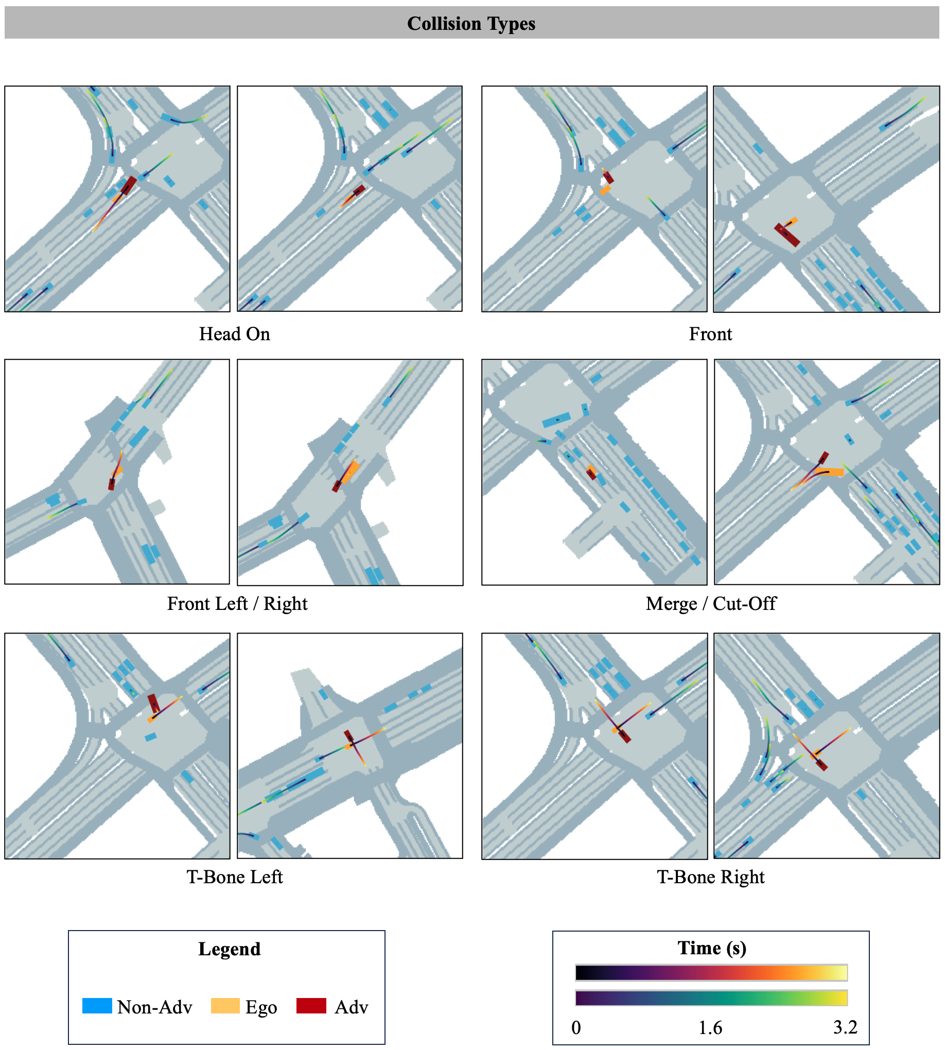
Figure 6: Example simulations of different collision types.

Moreover, our closed-loop method allows for longer simulation horizons compared to STRIVE, whose scenario length is constrained by the traffic motion model. As shown in Tab. 1, our method sustains its performance even when the scenario length is extended, maintaining lower realism and offroad occurrences, while effectively increasing the Ego-Adv collision rate. As illustrated in Figure 4, the qualitative examples from the NuScenes dataset demonstrate how our framework can challenge the rule-based planner with various driving situations. See Figs. 6 and 5 of the supplementary material for additional qualitative examples.

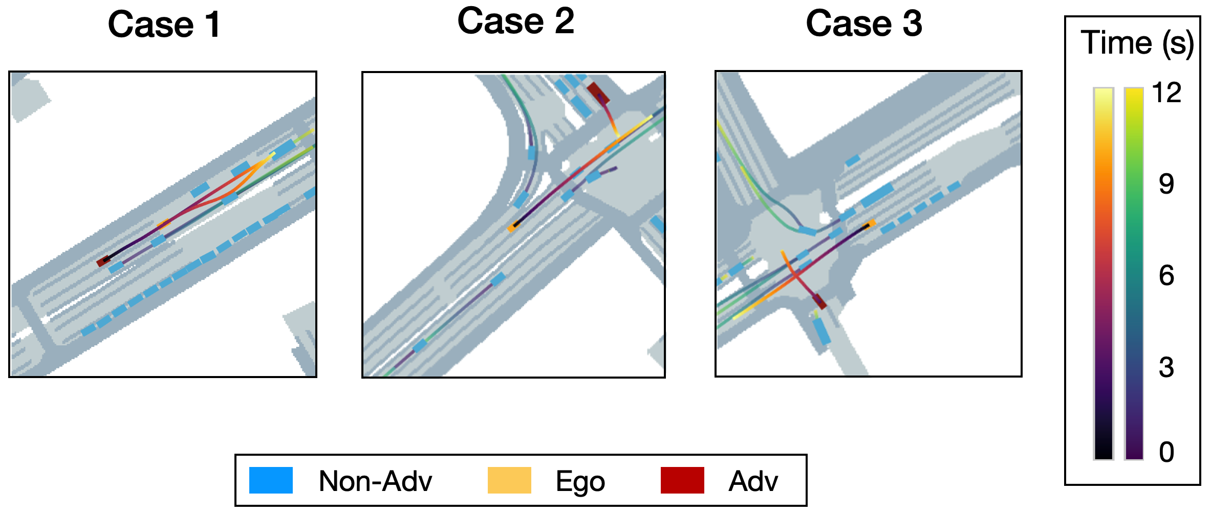
Figure 4: Qualitative Results of Rule-Based Planner on NuScenes Dataset. The depicted safety-critical scenarios demonstrate the framework’s capability to generate realistic and challenging long-tail situations for comprehensive planner assessment.

4.5 Safety-Critical Controllability Evaluation

Our method demonstrates enhanced controllability in generating adversarial scenarios compared to previous approaches. Specifically, we focus on controlling two critical aspects: the relative speed of the time-to-collision before the interaction between the ego and the adversarial vehicle.

Controlling Relative Speed. In our safety-critical simulation framework, we examine the effects of manipulating the desired relative speed between the ego vehicle and the adversarial agent. As shown in  Tab. 2, our proposed relative speed control results in a notable impact on both the actual ego-adversary relative speed and the collision rate. For instance, setting a lower desired relative speed target (-2.0 m/s) generally results in a decreased ego-adversary relative speed, and vice versa for a higher target (2.0 m/s). However, these adjustments do not directly translate to matching values in the simulations due to the nature of closed-loop interactions. The planner’s reactive behavior to the adversarial agent’s actions contributes to this discrepancy, as it may take evasive maneuvers or adjust its speed, potentially avoiding collisions altogether. Moreover, the realism metric across different relative speed settings remains relatively consistent, suggesting that the adjustments do not compromise the realism of the driving scenarios.

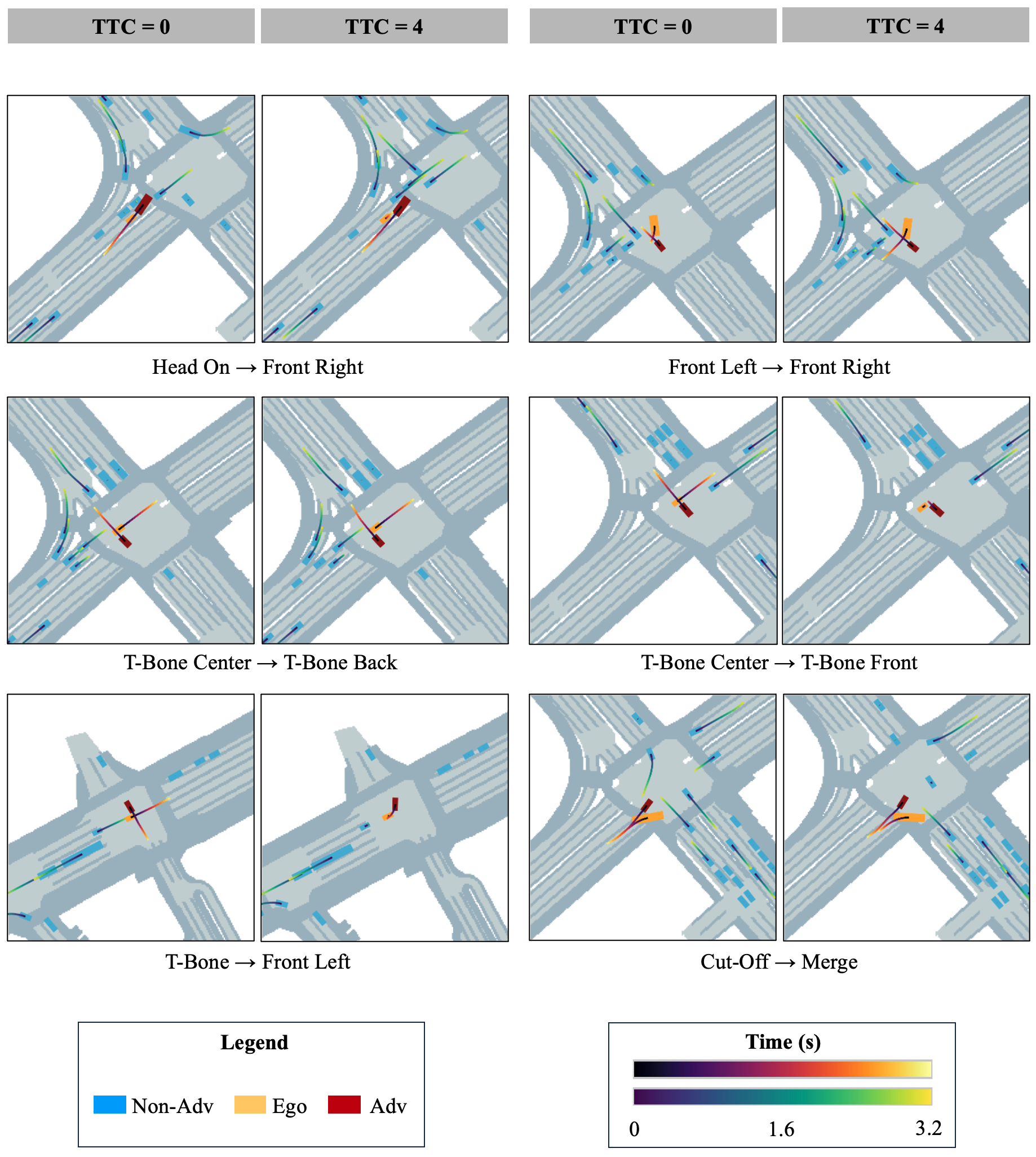
Figure 5: Example simulations showing the impact of time-to-collision control.

Controlling Time-to-Collision. In addition to relative speed, we control the orientation and relative speed together using the time-to-collision (TTC) cost, as described in Sec. 3.3. We manipulate the scenario’s safety-criticality by adjusting the relative weight of the TTC cost. To assess the impact of these adjustments, we measure the average TTC cost shortly before a collision occurs (0.5 seconds). Our observations, detailed in Tab. 3, show that increasing the TTC weight raises the TTC cost. Notably, while the relative collision speed remains fairly consistent, the collision angle shifts, indicating a higher difficulty in avoiding ego-adversary collisions. Based on qualitative examples in Fig. 5, these changing angles could potentially lead to more challenging cases for the ego vehicle, thereby enhancing the safety-critical aspect of the simulation.

4.6 Evaluation of Diffusion Model Performance in Closed-Loop Simulation

To evaluate our closed-loop traffic simulation framework, we utilized our diffusion model to control all agents within the scene for 20 seconds. We then benchmarked our model’s performance against the CTG model as reported in [2], with our results detailed in  Tab. 4. Note, since [2] does not report the performance of CTG when both collision and off-road guidance are employed, we implemented it ourselves and refer to it as CTG*. CTG* differs from our approach mainly in guidance functions and the adoption of clean guidance.

In practice, the diffusion model may encounter out-of-distribution challenges during closed-loop operation. Hence, the selection and implementation of effective guidance functions are crucial, particularly for tasks involving safety-critical simulations. As per the metrics in Tab. 4, our method demonstrates a significantly lower failure rate compared to both versions of CTG. Furthermore, the inclusion of route guidance functions in our model leads to a reduced rate of wrong-direction rate.

4.7 Ablation Study on Guidance Choices

We conducted an ablation study to evaluate the impact of various guidance choices in diffusion models on simulation quality. The study, summarized in  Tab. 5, involved replacing our proposed guidance functions and strategies with those originally used in CTG, such as the collision and road area loss functions, and omitting the clean guidance feature.

Effectiveness of Gaussian Collision Guidance ($J_{gc}$). The results demonstrate a significant reduction in the collision rate when using $J_{gc}$ compared to the original loss function. We attribute this improvement to $J_{gc}$’s enhanced signaling of potential collisions, accounting for both lateral and longitudinal components. This refined guidance ensures more realistic and safer interactions among vehicles.

Impact of Route Guidance ($J_{route}$). While the $J_{route}$ guidance did not substantially affect the off-road rate, it contributed to a lower rate of vehicles taking wrong directions. This outcome aligns with our goal of adhering to traffic rules, highlighting the importance of route-based guidance in maintaining traffic rule compliance within the simulation.

Influence of Clean Guidance. Omitting clean guidance led to scenarios where reactive agents frequently stopped on the road, as indicated by the reduced progress metric. Interestingly, other metrics like realism improved in these scenarios. Qualitatively, vehicles stopping on the road result in lower failure rates, and the realism metric tends to be better when vehicles exhibit minimal movement. The low acceleration and jerk will result in better realism when compared to the real-world log since most logged trajectories are low accelerations. This suggests that future efforts should focus on developing more comprehensive metrics to evaluate simulation quality.

5 Conclusion

In this work, we present a closed-loop simulation framework utilizing guided diffusion models for creating safety-critical scenarios to assess autonomous vehicle (AV) algorithms. Our framework introduces innovative guidance objectives, specifically tailored for stable, long-term safety-critical simulations. A key aspect of our approach is the formulation of adversarial objectives within the diffusion model’s output, enabling finely tuned control over adversarial behavior. Through extensive experimentation, we demonstrate that our framework offers better realism and controllability compared to previous adversarial scenario generation related works.

Future directions for our research include: 1) exploring the application of our framework in closed-loop policy training, and 2) developing automated methods for adjusting controllable parameters. These methods aim to facilitate the generation of diverse, long-tail scenarios. We believe this framework holds significant promise for enhancing real-world AV safety.

Supplementary Material

Method	Ego-Adv Coll	Ego-Other Coll	Other Offroad	Adv Offroad	Coll Speed	Realism
	(%) $\uparrow$	(%) $\uparrow$	(%) $\downarrow$	(%) $\downarrow$	(m/s) $\downarrow$	$\downarrow$
Ours (- $J_{route}$)	47.1	50.0	25.5	28.0	2.19	0.56
Ours  (- clean guide)	51.2	51.2	14.6	17.1	2.20	0.61
Ours	38.2	42.7	23.2	8.8	2.63	0.48

Table 6: Ablation study on diffusion model guidance functions for safety-critical simulation.We compare the performance of our approach with and without our proposed “route” and “clean” guidance functions when generating safety-critical traffic simulations. Our guidance lead to enhanced performance in Ego-Adversary collision rate with reduced adversary’s off-road rate and improved realism

Planner	Ego-Adv Coll	Ego-Other Coll	Adv Offroad	Coll Speed	Ego Accel	Realism
	(%) $\uparrow$	(%) $\uparrow$	(%) $\downarrow$	(m/s) $\downarrow$	(m/s2) $\downarrow$	$\downarrow$
BC	40.3	43.3	20.9	2.65	0.60	0.83
IDM	49.3	58.2	15.0	-0.37	1.09	0.85
Lane-graph	35.8	38.8	13.4	2.34	2.51	0.60

Table 7: Safety-Critical Simulation for different Planner settings

Table 8: Ablation Study on Accelerated Sampling through Different DDIM Steps. The table illustrates a performance degradation with fewer diffusion steps. Notably, DDIM with 10 steps still maintains a relatively low failure rate.

Method	Coll Rate	Off Road	Failure Rate	Wrong Direction	Progress	Realism
	(%) $\downarrow$	(%) $\downarrow$	(%) $\downarrow$	(%) $\downarrow$	(m) $\uparrow$	$\downarrow$
DDIM (10 steps)	3.58	5.34	8.78	16.97	65.4	0.93
DDIM (5 steps)	3.79	9.53	12.84	20.71	62.4	0.83
DDIM (1 step)	3.47	11.16	14.03	21.41	58.9	0.53
DDPM (100 steps)	1.74	4.40	6.05	9.73	51.3	0.88

6 Qualitative Results

We show two sets of qualitative results in the supplementary material. The first set, shown in Fig. 5, consists of a range of safety-critical simulations where varying the time-to-collision guidance changes the angle of collision. The second set, shown in Fig. 6, consists of example simulations of different types of collisions: T-Bone Right/Left, Merge, Front Right/Left, etc. Unlike STRIVE, which typically produces scenarios with limited variation, our approach can affect the collision angle, offering a more comprehensive range of safety-critical situations. This flexibility is particularly beneficial for testing and evaluating autonomous driving algorithms under various challenging conditions.

7 Importance of Our Guidances for Safety-Critical Simulation

We compare the performance of our approach with and without our proposed “route” and “clean” guidance functions when generating safety-critical traffic simulations, and report the results in Tab. 6. Although our guidance functions lead to lower performance in some metrics such as the Ego-Adv Collision rate, our approach with the addition of route guidance and clean guidances significantly reduces the Adv Off-Road rate to 8.8%. We argue this is an important choice, since the realistic behavior of all agents, including the adversarial vehicle, is crucial for safety-critical simulations. In effect, our guidance functions contribute to more realistic and plausible collision scenarios.

8 Safety-Critical Sim. for Different Planners

In Tab. 7, we present a comparison of different planner settings. Our evaluation includes a lane-graph-based planner mentioned in Sec. 4.2 as well as two other types of planners. The first is a deterministic Behavior Cloning (BC) planner, a learning-based approach that utilizes a ResNet Encoder from the diffusion model, followed by an MLP decoder to generate future trajectories. The second is an Intelligent Driver Model (IDM) planner [5], which uses the parameters: desired speed, acceleration, and safe distance to a lead car.

In Tab. 7, we demonstrate our framework’s ability to generate collisions across various planner types. Notably, the IDM planner exhibits the highest Ego-Adv collision rate. This heightened rate can be attributed to the IDM’s focus on vehicles near the same lane, potentially overlooking other vehicles in the scene. Consequently, in scenarios with the IDM planner, our framework can induce collisions at relatively lower speeds.

Conversely, the lane-graph-based planner demonstrates the lowest collision rate. This is likely due to its strategy of selecting lanes with minimal collision probabilities based on distance. Such a selection process inherently makes it more challenging for the adversarial agent to initiate collisions. In the future, our framework has the potential to be an invaluable tool for closed-loop policy training, particularly for learning-based planners. The adaptability of our framework to various planning strategies, coupled with its capability to generate realistic and safety-critical scenarios, is crucial for advancing the accuracy and reliability of autonomous driving algorithms.

9 Metrics Definitions

This section outlines the definitions of the metrics used in our evaluations, averaged across all scenarios, except for the realism metric.

9.1 Traffic Simulation Metrics

Off-road.

This metric measures the percentage of agents that go off-road in a given scenario. An agent is considered off-road if it moves into a non-drivable area.

Collision.

This metric represents the percentage of agents involved in collisions with other agents during the simulation.

Wrong Direction.

This metric quantifies the percentage of agents driving in the wrong direction. An agent is defined to be in the wrong direction if it deviates from the closest lane direction on the map by more than 90 degrees for a duration exceeding 0.3 seconds.

Realism.

Adopting the approach from [2], realism is quantified using the Wasserstein distance. This metric compares the normalized histograms of the driving profiles, focusing on the mean values of three key properties: longitudinal acceleration, lateral acceleration, and jerk. A lower value indicates a higher degree of realism.

Progress.

This metric measures the distance agents cover along their planned lanes, assessing their ability to navigate routes efficiently and consistently. Higher progress values reflect better adherence to traffic flow and lane paths, with fewer stops or deviations.

9.2 Adversarial Behavior and Collision Metrics

Collision Relative Speed.

Collision Relative Speed is defined as the ego planner’s speed minus the adversarial vehicle’s speed at the collision timestep.

To control the relative speed, we introduce the relative speed cost function:

$$J_{v}=\sum_{t=1}^{T}|v^{1}_{t}-v^{a}_{t}-v_{\text{diff}}|\cdot\mathbf{1}{\{d(t)<d_{\text{col}}\}},$$ (10)

where $v_{\text{diff}}$ is the desired speed difference between the ego and the adversarial vehicles, influencing the relative speed at the point of collision. The function $\mathbf{1}{\{d(t)<d_{\text{col}}\}}$ is an indicator function that applies the cost only when the distance $d(t)$ between the ego and adversarial vehicle is less than a specified threshold $d_{\text{col}}$.

Time-to-Collision Cost.

The Time to Collision (TTC) cost [28] assesses collision risk based on the relative speed and orientation between agents. For two agents located at positions $(x_{i},y_{i})$ and $(x_{j},y_{j})$ with respective velocities $(v_{x_{i}},v_{y_{i}})$ and $(v_{x_{j}},v_{y_{j}})$, we define their relative position and velocity. The relative position is given by $dx=x_{i}-x_{j}$ and $dy=y_{i}-y_{j}$, representing the positional differences along the x and y axes. Similarly, the relative velocity is calculated as $dv_{x}=v_{x_{i}}-v_{x_{j}}$ and $dv_{y}=v_{y_{i}}-v_{y_{j}}$, which are the differences in their velocities along the x and y axes. The TTC is computed under a constant velocity assumption, solving a quadratic equation to find the time of collision $t_{\text{col}}$, with a collision considered when relative distance is minimal.

The real part of the solution provides the time to the point of closest approach, $\tilde{t}_{\text{col}}$, calculated as:

$$\tilde{t}_{\text{col}}=\begin{cases}-\frac{dv_{x}dx+dv_{y}dy}{\tilde{dv}^{2}}&\text{if }\tilde{t}_{\text{col}}\geq 0,\\ 0&\text{otherwise},\end{cases}$$ (11)

and the distance at that time, $\tilde{d}_{\text{col}}$, is given by:

$$\tilde{d}_{\text{col}}^{2}=\begin{cases}\frac{(dv_{x}dy-dv_{y}dx)^{2}}{\tilde{dv}^{2}}&\text{if }\tilde{t}_{\text{col}}\geq 0,\\ dx^{2}+dy^{2}&\text{otherwise}.\end{cases}$$ (12)

We define the TTC cost $J_{\text{ttc}}$ as:

$$J_{\text{ttc}}=\sum_{t=1}^{T}-\exp\left(-\frac{\tilde{t}_{\text{col}(t)}^{2}}{2\lambda_{t}}-\frac{\tilde{d}_{\text{col}(t)}^{2}}{2\lambda_{d}}\right),$$ (13)

where $\lambda_{t}$ and $\lambda_{d}$ are the time and distance bandwidth parameters. This cost is evaluated over a time horizon $T$, with a higher cost for scenarios having low time to collision and proximity. For further details on the derivation of this cost function, we direct readers to [28].

In our evaluations, we focus on the average TTC cost of 0.5 seconds preceding a collision. This metric effectively captures the criticality of the safety scenarios, reflecting the potential risk of imminent collisions.

Time-to-Collision.

Additionally, we compute the average Time-to-Collision (TTC) for each timestep within the crucial 0.5-second window before collisions occur in our scenarios. It’s important to note that this TTC is not the actual time until a collision, but rather a theoretical estimate based on the constant velocity model assumption for each timestep.

10 Implementation Details

In this section, we discuss the implementation details of our diffusion model, focusing on the hyperparameters used during training.

10.1 Diffusion Process Details

For the diffusion process, we utilize a cosine variance schedule as described in [1], with the number of diffusion steps set to $K=100$. The variance scheduler parameters are configured with a lower bound $\beta_{1}$ of 0.0001 and an upper bound $\beta_{K}$ of 0.05. The diffusion model takes in a 1-second history and is trained to predict the next 3.2 seconds with a step time $dt=0.1$. Our model was trained on four NVIDIA RTX A6000 GPUs for 70000 iterations using the Adam optimizer, with a learning rate set to $1\times 10^{-5}$. The diffusion model’s implementation is based on methodologies from open-source repositories [1][30], and the simulation framework is developed based on [31][26].

10.2 Guidance details

To simultaneously incorporate multiple guidance functions in our model, we assign weights to balance their contributions. In our experiments, particularly with non-adversarial agents, we implement a combination of route guidance ($J_{\text{route}}$) and Gaussian collision guidance ($J_{\text{gc}}$) across $M=20$ examples. Notably, we apply a filtration process exclusively to $J_{\text{gc}}$, aiming to prevent imminent collisions For adversarial agents, we maintain the same weighting across all guidance functions, but uniquely control the weighting for $J_{\text{ttc}}$ to achieve controllable behavior. In this setting, we select the sample that yields the highest adversarial cost ($J_{\text{adv}}$), ensuring effective and targeted adversarial scenarios.

10.3 Accelerated Sampling and Parameterization

In each denoising step, our model predicts the mean of the next denoised action trajectory Eq. 3. Instead of predicting the noise $\epsilon$ that is used to corrupt the trajectory [30], we directly output the denoised clean trajectory $\hat{\tau}_{0}$ [2][24]. The predicted mean based on $\hat{\tau}_{0}$ and ${\tau}_{k}$:

$$\tau_{k-1}=\mu_{\theta}(\tau_{k},\hat{\tau}_{0})=\frac{\sqrt{\bar{\alpha}_{k-1}}\beta_{k}}{1-\bar{\alpha}_{k}}\hat{\tau}_{0}+\frac{\sqrt{\alpha_{k}}(1-\bar{\alpha}_{k-1})}{1-\bar{\alpha}_{k}}\tau_{k}$$ (14)

where $\beta_{k}$ represents the variance from the noise schedule in the diffusion process, $\alpha_{k}$ is defined as $\alpha_{k}:=1-\beta_{k}$, indicating the incremental noise reduction at each step, and $\bar{\alpha}_{k}$ is the cumulative product of $\alpha_{j}$ up to step $k$, mathematically expressed as $\bar{\alpha}_{k}=\prod_{j=0}^{k}\alpha_{j}$.

In future work, accelerating the diffusion process is vital, particularly for closed-loop policy training. One promising method is the Denoising Diffusion Implicit Models (DDIM) approach, which notably speeds up the sampling in diffusion models[32]. Given a diffusion process with a total of $K$ steps, denoted as $k=\{1,\ldots,K\}$, DDIM achieves acceleration by selecting a sub-sequence $\hat{k}$, which is a subset of $\{1,\ldots,K\}$ chosen with a specific stride.

For each step in the sub-sequence $\hat{k}$, the predicted mean is calculated using:

$$\tau_{\hat{k}-1}=\sqrt{\bar{\alpha}_{\hat{k}-1}}\cdot\hat{\tau}_{0}+\sqrt{1-\bar{\alpha}_{\hat{k}-1}}\cdot\hat{\epsilon}$$ (15)

where the predicted noise $\hat{\epsilon}$ in this accelerated process can be derived as follows:

$$\tau_{k} =\sqrt{\bar{\alpha}_{k}}\hat{\tau}_{0}+\sqrt{1-\bar{\alpha}_{k}}\hat{\epsilon},$$ (16)

$$\hat{\epsilon} =\frac{\tau_{k}-\sqrt{\bar{\alpha}_{k}}\hat{\tau}_{0}}{\sqrt{1-\bar{\alpha}_{k}}}.$$

This accelerated sampling approach significantly reduces the number of steps needed to generate samples from the diffusion model, thereby speeding up the simulation process. The results of our ablation study, as detailed in Tab. 8, reveal a performance trade-off with this method. While most metrics experience a decline, the reduction in diffusion steps to 10 in DDIM still yields a comparably low failure rate. Interestingly, a single DDIM step results in the best realism score. These findings highlight the potential of accelerated sampling in diffusion models, particularly for applications in closed-loop policy training, where simulation speed is crucial.

References

- [1] Michael Janner, Yilun Du, Joshua B Tenenbaum, and Sergey Levine. Planning with diffusion for flexible behavior synthesis. arXiv preprint arXiv:2205.09991, 2022.
- [2] Ziyuan Zhong, Davis Rempe, Danfei Xu, Yuxiao Chen, Sushant Veer, Tong Che, Baishakhi Ray, and Marco Pavone. Guided conditional diffusion for controllable traffic simulation. In 2023 IEEE International Conference on Robotics and Automation (ICRA), pages 3560–3566. IEEE, 2023.
- [3] Davis Rempe, Zhengyi Luo, Xue Bin Peng, Ye Yuan, Kris Kitani, Karsten Kreis, Sanja Fidler, and Or Litany. Trace and pace: Controllable pedestrian animation via guided trajectory diffusion. In Proceedings of the IEEE/CVF Conference on Computer Vision and Pattern Recognition, pages 13756–13766, 2023.
- [4] Holger Caesar, Varun Bankiti, Alex H Lang, Sourabh Vora, Venice Erin Liong, Qiang Xu, Anush Krishnan, Yu Pan, Giancarlo Baldan, and Oscar Beijbom. nuscenes: A multimodal dataset for autonomous driving. In Proceedings of the IEEE/CVF conference on computer vision and pattern recognition, pages 11621–11631, 2020.
- [5] Martin Treiber, Ansgar Hennecke, and Dirk Helbing. Congested traffic states in empirical observations and microscopic simulations. Physical review E, 62(2):1805, 2000.
- [6] Holger Caesar, Varun Bankiti, Alex H. Lang, Sourabh Vora, Venice Erin Liong, Qiang Xu, Anush Krishnan, Yu Pan, Giancarlo Baldan, and Oscar Beijbom. nuscenes: A multimodal dataset for autonomous driving. arXiv preprint arXiv:1903.11027, 2019.
- [7] Simon Suo, Sebastian Regalado, Sergio Casas, and Raquel Urtasun. Trafficsim: Learning to simulate realistic multi-agent behaviors. In Proceedings of the IEEE/CVF Conference on Computer Vision and Pattern Recognition, pages 10400–10409, 2021.
- [8] Danfei Xu, Yuxiao Chen, Boris Ivanovic, and Marco Pavone. Bits: Bi-level imitation for traffic simulation. In 2023 IEEE International Conference on Robotics and Automation (ICRA), pages 2929–2936. IEEE, 2023.
- [9] Midjourney. https://www.midjourney.com. Accessed: 2023-11-16.
- [10] Openai dall-e-2. https://openai.com/product/dall-e-2. Accessed: 2023-11-16.
- [11] Robin Rombach, Andreas Blattmann, Dominik Lorenz, Patrick Esser, and Björn Ommer. High-resolution image synthesis with latent diffusion models. In Proceedings of the IEEE/CVF conference on computer vision and pattern recognition, pages 10684–10695, 2022.
- [12] Prafulla Dhariwal and Alexander Nichol. Diffusion models beat gans on image synthesis. Advances in neural information processing systems, 34:8780–8794, 2021.
- [13] Jonathan Ho and Tim Salimans. Classifier-free diffusion guidance. arXiv preprint arXiv:2207.12598, 2022.
- [14] Jonathan Ho, William Chan, Chitwan Saharia, Jay Whang, Ruiqi Gao, Alexey Gritsenko, Diederik P Kingma, Ben Poole, Mohammad Norouzi, David J Fleet, et al. Imagen video: High definition video generation with diffusion models. arXiv preprint arXiv:2210.02303, 2022.
- [15] Niklas Hanselmann, Katrin Renz, Kashyap Chitta, Apratim Bhattacharyya, and Andreas Geiger. King: Generating safety-critical driving scenarios for robust imitation via kinematics gradients. In European Conference on Computer Vision, pages 335–352. Springer, 2022.
- [16] Yulong Cao, Chaowei Xiao, Anima Anandkumar, Danfei Xu, and Marco Pavone. Advdo: Realistic adversarial attacks for trajectory prediction. In European Conference on Computer Vision, pages 36–52. Springer, 2022.
- [17] Jingkang Wang, Ava Pun, James Tu, Sivabalan Manivasagam, Abbas Sadat, Sergio Casas, Mengye Ren, and Raquel Urtasun. Advsim: Generating safety-critical scenarios for self-driving vehicles. In Proceedings of the IEEE/CVF Conference on Computer Vision and Pattern Recognition, pages 9909–9918, 2021.
- [18] Yasasa Abeysirigoonawardena, Florian Shkurti, and Gregory Dudek. Generating adversarial driving scenarios in high-fidelity simulators. In 2019 International Conference on Robotics and Automation (ICRA), pages 8271–8277. IEEE, 2019.
- [19] Qingzhao Zhang, Shengtuo Hu, Jiachen Sun, Qi Alfred Chen, and Z Morley Mao. On adversarial robustness of trajectory prediction for autonomous vehicles. In Proceedings of the IEEE/CVF Conference on Computer Vision and Pattern Recognition, pages 15159–15168, 2022.
- [20] Zhao-Heng Yin, Lingfeng Sun, Liting Sun, Masayoshi Tomizuka, and Wei Zhan. Diverse critical interaction generation for planning and planner evaluation. In 2021 IEEE/RSJ International Conference on Intelligent Robots and Systems (IROS), pages 7036–7043. IEEE, 2021.
- [21] Chejian Xu, Ding Zhao, Alberto Sangiovanni-Vincentelli, and Bo Li. Diffscene: Diffusion-based safety-critical scenario generation for autonomous vehicles. In The Second Workshop on New Frontiers in Adversarial Machine Learning, 2023.
- [22] Davis Rempe, Jonah Philion, Leonidas J Guibas, Sanja Fidler, and Or Litany. Generating useful accident-prone driving scenarios via a learned traffic prior. In Proceedings of the IEEE/CVF Conference on Computer Vision and Pattern Recognition, pages 17305–17315, 2022.
- [23] Jonathan Ho, Ajay Jain, and Pieter Abbeel. Denoising diffusion probabilistic models. Advances in neural information processing systems, 33:6840–6851, 2020.
- [24] Alexander Quinn Nichol and Prafulla Dhariwal. Improved denoising diffusion probabilistic models. In International Conference on Machine Learning, pages 8162–8171. PMLR, 2021.
- [25] Chiyu Jiang, Andre Cornman, Cheolho Park, Benjamin Sapp, Yin Zhou, Dragomir Anguelov, et al. Motiondiffuser: Controllable multi-agent motion prediction using diffusion. In Proceedings of the IEEE/CVF Conference on Computer Vision and Pattern Recognition, pages 9644–9653, 2023.
- [26] Danfei Xu, Yuxiao Chen, Boris Ivanovic, and Marco Pavone. Bits: Bi-level imitation for traffic simulation. In 2023 IEEE International Conference on Robotics and Automation (ICRA), pages 2929–2936. IEEE, 2023.
- [27] Simon Suo, Kelvin Wong, Justin Xu, James Tu, Alexander Cui, Sergio Casas, and Raquel Urtasun. Mixsim: A hierarchical framework for mixed reality traffic simulation. In Proceedings of the IEEE/CVF Conference on Computer Vision and Pattern Recognition, pages 9622–9631, 2023.
- [28] Haruki Nishimura, Jean Mercat, Blake Wulfe, Rowan Thomas McAllister, and Adrien Gaidon. Rap: Risk-aware prediction for robust planning. In Conference on Robot Learning, pages 381–392. PMLR, 2023.
- [29] Kaiming He, Xiangyu Zhang, Shaoqing Ren, and Jian Sun. Deep residual learning for image recognition. In Proceedings of the IEEE conference on computer vision and pattern recognition, pages 770–778, 2016.
- [30] Tianpei Gu, Guangyi Chen, Junlong Li, Chunze Lin, Yongming Rao, Jie Zhou, and Jiwen Lu. Stochastic trajectory prediction via motion indeterminacy diffusion. In Proceedings of the IEEE/CVF Conference on Computer Vision and Pattern Recognition, pages 17113–17122, 2022.
- [31] Boris Ivanovic, Guanyu Song, Igor Gilitschenski, and Marco Pavone. trajdata: A unified interface to multiple human trajectory datasets. arXiv preprint arXiv:2307.13924, 2023.
- [32] Jiaming Song, Chenlin Meng, and Stefano Ermon. Denoising diffusion implicit models. arXiv preprint arXiv:2010.02502, 2020.