Magnon, doublon and quarton excitations in 2D trimerized Heisenberg models

Abstract

We investigate the magnetic excitations of the trimerized Heisenberg models with intra-trimer interaction $J_{1}$ and inter-trimer interaction $J_{2}$ on four different two-dimensional lattices using a combination of stochastic series expansion quantum Monte Carlo (SSE QMC) and stochastic analytic continuation methods (SAC), complemented by cluster perturbation theory (CPT). These models exhibit quasi-particle-like excitations when $g=J_{2}/J_{1}$ is small, characterized by low-energy magnons, intermediate-energy doublons, and high-energy quartons. The low-energy magnons are associated with the magnetic ground states. They can be described by the linear spin wave theory (LSWT) of the effective block spin model and the original spin model. Doublons and quartons emerge from the corresponding internal excitations of the trimers with distinct energy levels, which can be effectively analyzed using perturbation theory when the ratio of exchange interactions $g$ is small. In this small $g$ regime, we observe a clear separation between the magnon and higher-energy spectra. However, as $g$ increases, these three spectra gradually merge into the magnon modes or continua. Nevertheless, the LSWT fails to provide quantitative descriptions of the higher-energy excitation bands due to significant quantum fluctuations. Notably, in the Collinear II and trimerized hexagon lattice, a broad continuum emerges above the single-magnon spectrum, originating from the quasi-1D physics due to the dilute connections between chains. Our numerical analysis of these 2D trimers yields valuable theoretical predictions and explanations for the inelastic neutron scattering (INS) spectra of 2D magnetic materials featuring trimerized lattices.

I Introduction

Elementary excitations  [1, 2] are key to understanding the physical properties of magnetic systems. In systems with long-range magnetic orders, the linear spin wave theory (LSWT) is commonly employed to investigate the corresponding magnetic excitations  [3, 4]. For example, the LSWT can fit the result of inelastic neutron scattering experiments on La₂CuO₄, which is the parent compound of cuprate superconductors  [5, 6]. Nonetheless, when quantum fluctuations are notably strong or when various types of excitations happen simultaneously, the accuracy of LSWT results is challenged, even in situations where the ground state retains magnetic order. For example, LSWT cannot adequately predict the continuum at the momentum point $(\pi,0)$ in the square-lattice Heisenberg model  [7, 8], which is relevant to the inelastic neutron scattering of Cu(DCOO)₂ $\cdot$ 4D₂O. In contrast, unbiased numerical simulations play a pivotal role in exploring magnetic excitations in quantum many-body systems  [9, 10, 11]. Among these numerical techniques, the combination of large-scale quantum Monte Carlo with stochastic analytical continuation is a powerful technique in investigating magnetic excitations, as it can faithfully reproduce the inelastic neutron scattering spectra  [12, 13].

Previous studies by some of our authors and collaborators have unveiled novel excitations in magnetically ordered systems featuring square-lattice-like  [14, 15, 16, 17, 18], where the LSWT fails to predict some high-energy excitations. They further studied a trimer chain system in Ref.  [19], and discovered two new forms of excitations above the low-energy two-spinon continuum, named “doublon” and “quarton”. Soon after that, experiments on Na₂Cu₃Ge₄O₁₂ confirmed these theoretical predictions  [20], where neutron experiments revealed these two excitations. Moreover, introducing an additional magnetic field to the trimer chain system induces $XY$ and $1/3$ magnetization plateau phases, and the doublon and quarton are still observable when $g$ is small [21].

In two-dimensional (2D) systems, some materials also have trimerized structures, as evidenced in some experimental studies, including compounds like CaNi₃(P₂O₇)₂, Ba₄Ir₃O₁₀, and Ba₄Ru₃O₁₀  [22, 23, 24, 25]. Unlike the 1D chain, 2D trimer systems can exhibit magnetic ground states with magnons as their low-energy excitations. When the interactions between trimers (or $g=J_{2}/J_{1}$) are relatively small, the presence of doublons and quartons can be expected. Therefore, it is of great interest to explore how magnons, doublons, and quartons evolve as the ratio $g$ changes.

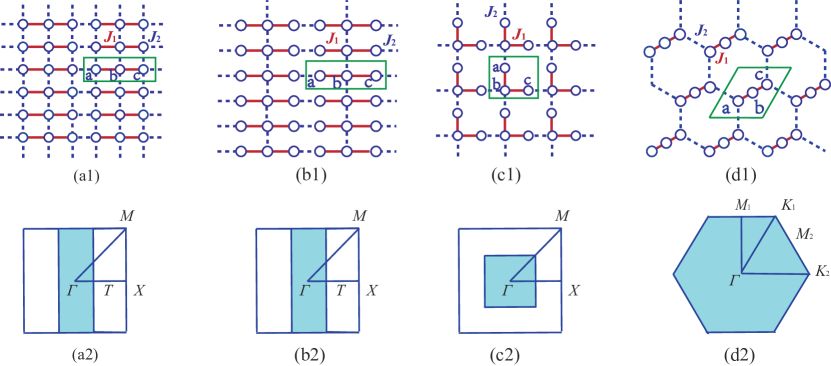
Figure 1: Four 2D trimerized lattices and their full Brillouin zones: (a1) Collinear I lattice, (b1) Collinear II lattice, (c1) Trimerized Lieb lattice, (d1) Trimerized hexagon lattice, in which the green quadrilaterals represent unit cells. The Collinear I lattice comprises three sites and six bonds within a cell, while the other lattices feature three sites and four bonds per cell. The red bonds denote the intra-trimer interactions, while the dark blue ones represent the inter-trimer interactions. It is worth noting that all these neighbor bonds are antiferromagnetic interactions. For (a1)-(c1), the length between $a$ and $b$ sublattices within a unit cell is set to be one, and the lengths of blue dashed lines are also equal to one. While in the (d1) lattice, we set the length between $a$ and $c$ sublattices within a unit cell to be two. For panels (a2)-(d2), we illustrate the corresponding full Brillouin zone (BZ), and the shadow areas denote the reduced BZ. The point $T$ is $(2\pi/3,0)$ and point $M_{2}$ is $(\sqrt{3}\pi/6,\pi/6)$.

In our study, we consider 2D trimerized models on four lattices including the Collinear I, Collinear II, trimerized Lieb lattice, and trimerized hexagon lattice, which are shown in Figs. 1(a1)-(d1). These models all share a common characteristic: they feature intra-trimer exchange interaction represented by $J_{1}$ and inter-trimer exchange interaction labeled as $J_{2}$. It is noteworthy that some of the lattices have been synthesized in real materials  [22, 23]. All of these lattices consist of trimer blocks with $a$, $b$, and $c$ sublattices, as depicted in Figs. 1(a1) to  1(d1). A slight distinction among these lattices is that the last one exhibits a hexagon structure, while the others are arranged like a square lattice. This hexagon trimerized lattice can be also topologically deformed to a kind of bond-depleted square lattice similar to Collinear II.

In this paper, we focus on the study of dynamic spin structure factors, denoted as $S(q,\omega)$, for four trimerized Heisenberg models with varying ratios $g=J_{2}/J_{1}$. To calculate this quantity, we use the stochastic series expansion quantum Monte Carlo (SSE-QMC) combined with the stochastic analytic continuation (SAC) method  [26, 27, 28, 29, 30], which has gained a lot of improvement in recent years and has been successfully applied to many systems. Meanwhile, we also use the cluster perturbation theory (CPT) with exact diagonalization (ED) as a solver to supplement QMC results. In the 2D trimer models, unlike the 1D trimer chain which exhibits two-spinon continuum behavior, the low-energy part is now dominated by magnons. For these low-energy magnons, we employ perturbation theory to derive the effective models among block spins formed by the trimer doublets  [31]. Subsequently, we can apply linear spin wave theory (LSWT) to the effective models and get the dispersions of low-energy magnons  [32]. Regarding doublons and quartons, we use perturbation analysis to extract their dispersion relations  [33], which is a suitable approach to fit the $S(q,\omega)$ spectra for small $g$. However, as $g$ gradually increases, the doublons and quartons can merge into magnon modes or become continua. Especially, the Collinear II and the trimerized hexagon lattice maintain more features from the trimer chain, resulting in high-energy broad continua. The trimerized Lieb lattice keeps its three separated energy bands in the range of $g\in(0,1]$ for the CPT results, while the QMC results have some continua near point $X$. We attribute this to the finite clusters used in the CPT calculations. Through a combination of numerical simulations and theoretical analyses, our research provides a comprehensive study of the excitation dynamics of 2D trimer models. Our study can give a deeper understanding of the excitation mechanisms in 2D trimer block systems and the corresponding materials.

We have structured this paper as follows. In Sec. II, we provide an introduction to four 2D trimerized models featuring antiferromagnetic interactions, along with a brief overview of the numerical techniques employed. Moving on to Sec. III, we present the spectra of these trimer systems and draw comparisons between the LSWT data and the SAC results. In Sec. IV, we focus on the analysis of quasi-particles at various energy levels, including magnons, doublons, and quartons. Finally, in Sec. V, we summarize the discussion of our studies and some of our plans for the future.

II Models and Methods

II.1 Model Hamiltonian

In this paper, we thoroughly explore the isotropic Heisenberg model on four distinct 2D trimerized lattices, illustrated in Figs. 1(a1)-(d1). Each lattice features two kinds of nearest-neighbor exchange interactions, denoted as $J_{1}$ and $J_{2}$. The Hamiltonian for these systems is given by

$$H={J_{1}}\sum\limits_{\left\langle{i,j}\right\rangle}{{S_{i}}\cdot}{S_{j}}+{J_{2}}\sum\limits_{\left\langle{i,j}\right\rangle^{\prime}}{{S_{i}}\cdot}{S_{j}},$$ (1)

where $S_{i}$ represents the spin operator at site $i$, $J_{1}$ and $J_{2}$ stand for the intratrimer and intertrimer coupling strengths, respectively. We also denote the first term (include $J_{1}$) as $H_{t}$ which means interactions in a trimer, and white the second term (include $J_{2}$) as $H_{tt}$ which means interactions between two trimers). For simplicity, we define the coupling ratio as $g=J_{2}/J_{1}$, where $g=0$ corresponds to the decoupled trimer limit and $g=1$ represents the uniform cases. We set $J_{1}=1$ as the energy unit, and let $g$ vary in the range of $(0,1]$ to explore the dynamic spin structure factors. The first three lattices depicted in Figs. 1(a1)- 1(c1) exhibit square-lattice-like structures, respectively named Collinear I, Collinear II, and trimerized Lieb lattice, and the last one in Fig. 1(d1) presents a hexagon configuration, named trimerized hexagon lattice. The corresponding full BZs are shown in panels Figs. 1(a2)-(d2), and the reduced BZs are illustrated in shadow areas.

In this paper, we mainly focus on the magnetic excitations of these four trimerized lattice models. The magnetic excitation spectra with $\Delta S=1$ can be well revealed by the dynamic spin structure factors $S(q,\omega)$, and can be detected by the inelastic neutron scattering experiment. To calculate this quantity, we mainly use two kinds of methods, QMC and CPT. Each method has its advantages and disadvantages. In addition, we also use LSWT to analyze the low-energy magnon and use perturbation theory to get the dispersions of doublon and quarton. In the following, we mainly introduce the QMC and CPT methods.

II.2 Quantum Monte Carlo

QMC can be simulated on the large-scale lattice, thereby capturing more information on long-range correlation and entanglement  [34]. However, this method does not provide direct access to real-time or real-frequency dynamic correlation functions. Instead, these functions are obtained through analytical continuation from imaginary-time Green functions. With the development of powerful stochastic analytical continuation methods  [26, 27, 28, 29, 30, 35, 36, 37, 38, 39, 40], researchers have continually improved their computational ability.

To obtain the dynamic spin structure factors using QMC, we start by obtaining the imaginary-time correlation functions through SSE-QMC samplings. These correlation functions are defined as ${G_{q}}(\tau)=3\left\langle S_{-q}^{z}(\tau)S_{q}^{z}(0)\right\rangle$, where the factor of $3$ arises from the $SU(2)$ continuous symmetry of isotropic Heisenberg model, and $S_{q}^{z}$ represents the Fourier transform of the $z$-component spin operator, which can be written as:

$$S_{q}^{z}=\frac{1}{{\sqrt{N}}}\sum\limits_{i=1}^{N}{{e^{-i{{\vec{r}}_{i}}\cdot\vec{q}}}S_{i}^{z}},$$ (2)

where ${\vec{r}}_{i}$ is the displacement of site $i$. To visualize the $S(q,\omega)$, we follow a high-symmetry path $\Gamma(0,0)$ $\rightarrow$ $T(2\pi/3,0)$ $\rightarrow$ $X(\pi,0)$ $\rightarrow$ $M(\pi,\pi)$ $\rightarrow$ $\Gamma(0,0)$ for three square-lattice-like models, as depicted in Figs. 1(a1)-(c1). We use the full BZ for these lattices when employing the QMC procedure. However, for the trimerized hexagon lattice, we employ the dynamic spin structure factors in the reduced BZ which is shown in  1(d4):

$$S_{red}^{zz}(q,\omega)=\sum\limits_{\alpha=a,b,c}{S_{\alpha\alpha}^{zz}(q,\omega)},$$ (3)

where $S_{\alpha\alpha}^{zz}(q,\omega)$ is the dynamic structure factors which only consider the spins at sites $\alpha\in{a,b,c}$, and we choose the path $\Gamma(0,0)$ $\rightarrow$ $M_{1}(0,\pi/3)$ $\rightarrow$ $K_{1}(\sqrt{3}\pi/9,\pi/3)$ $\rightarrow$ $\Gamma(0,0)$ $\rightarrow$ $K_{2}(2\sqrt{3}\pi/9,0)$ $\rightarrow$ $M_{2}(\sqrt{3}\pi/6,\pi/6)$ $\rightarrow$ $K_{1}(\sqrt{3}\pi/9,\pi/3)$. The connection between ${G_{q}}(\tau)$ and the dynamic spin structure factors $S(q,\omega)$ is established through analytical continuation, which is expressed by the following equation,

$${G_{q}}(\tau)=\frac{1}{\pi}\int_{-\infty}^{\infty}{d\omega S(q,\omega){e^{-\tau\omega}}}.$$ (4)

To tackle this inverse problem, in the SAC procedure, we parameterize $S(q,\omega)$ by employing multiple $\delta$ functions and adjusting both their amplitudes and frequencies. Stochastic averaging of the configurations balancing $\left\langle\chi^{2}\right\rangle$ minimization and sampling entropy provides converged results of the spectral functions  [41]. In this work, our calculations for the dynamic spin structure factors are conducted on $L_{x}\times L_{y}$ trimer blocks, with $L_{y}=3L_{x}=48$ for the two collinear models and $L_{y}=L_{x}=24$ for the trimerized Lieb lattice and trimerized hexagon lattice.

In this paper, we present the excitation spectra of four trimerized models using QMC-SAC and CPT methods, and we further analyze the magnon, doublon, and quarton using LSWT and perturbation theory. In our QMC-SAC calculations, we set the inverse temperature up to $\beta=256$, allowing us to utilize about 100 discrete $\tau$ in the SAC procedure.

II.3 Cluster Perturbation Theory

Cluster perturbation theory (CPT) offers an alternative method for obtaining $S(q,\omega)$ without the need for analytical continuation. CPT employs exact diagonalization (ED) as a solver and has been successfully applied in the study of several spin models  [42, 43, 44]. In this approach, ED is employed to investigate the dynamic correlation effects in the clusters, while perturbation and mean-field theories are utilized to deal with the inter-cluster interactions and correlations. Within the CPT framework, we focus on calculating the transverse dynamic spin structure denoted as ${S^{+-}}(q,\omega)$. In 2D trimer models with $SU(2)$ symmetry, ${S^{+-}}(q,\omega)$ are consistent with $S^{zz}(q,\omega)$.

For the CPT method with ED as a solver, the cluster size is limited. We use the clusters with $L_{y}=2L_{x}=4$ for two collinear trimerized models and $L_{x}=L_{y}=3$ for the trimerized Lieb lattice. Within clusters, both local and non-local dynamic correlations are treated exactly. However, non-local correlations between clusters are addressed using perturbation and mean-field theory. It is worth noting that the mean-field treatment tends to overestimate magnetic ordering  [45, 46], implying a potential underestimation of quantum fluctuations. Nevertheless, this method yields nearly exact results within certain limits. The first limit is that the cluster is infinitely large. This allows for the convergence results with increasing cluster sizes, which is more efficient than calculations with finite-size torus geometries  [47]. Another exact limit occurs when the interactions between clusters are infinitely small, making perturbation theory work well. Therefore, the CPT method is very suitable to analyze the excitations in small $g$.

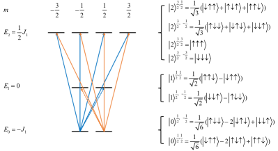
Figure 2: The energy levels and the corresponding wave functions of an isolated trimer block. Its ground state is a doublet with effective spin-$1/2$. $\left|n\right\rangle^{S,m}$ denotes an eigenstate, where $n=0,1,2$ represents the ground state, first excited state, and second excited state, respectively. $S$ is the total spin quantum number and $m$ is the magnetic quantum number. The dashed lines denote the $|\Delta m|=1$ excitations and the solid lines are $|\Delta S|=1$ excitations. The orange lines denote the excitations from $\left|0\right\rangle^{\frac{1}{2},\frac{1}{2}}$ ground state and the blue lines are the excitations from $\left|0\right\rangle^{\frac{1}{2},-\frac{1}{2}}$ ground state.

III Numerical Results

When $g=0$, all four models are fully decoupled, and each trimer block forms a doublet with effective block spin $S=1/2$. The energy levels of a single trimer have been previously depicted in Ref  [19], which are also shown diagrammatically in Fig. 2. The ground state and the first excited state are both doublets with the magnetic quantum number $m=\pm 1/2$, and the second excited state is a quartet with $m=\pm 3/2$. Fig. 2 also illustrates the $|\Delta S|=1$ (quarton excitations, solid arrow lines) and $|\Delta m|=1$ ($|\Delta S|=0$, doublon excitations, dashed arrow lines) excitations of a single trimer, which can be used to explore the dispersions of quasiparticles using perturbation theory. As we turn on small values of $g$, the low-energy excitations are dominated by the effective block spin models, which will be analyzed in detail in Sec. IV.

Specifically, the introduction of $J_{2}$ enables the excitation from the ground-state doublet to the first-excited doublet, to propagate as a quasi-particle moving on the lattices. We refer to this quasi-particle as a doublon, inherited from the 1D trimer chain [48]. Similarly, for the doublet to quartet excitation, the introduction of $J_{2}$ also induces the quasiparticle named quarton to propagate in the 2D lattices. The doublon and quarton have their typical energy scales for spin-$1/2$ systems, $J_{1}$ and $1.5J_{1}$ respectively. As we vary the value of $g$, how the low-energy magnon, intermediate-energy doublon, and high-energy quarton evolve is much less known. Under small $g$, we can see the separation of doublon and quarton in the CPT spectrum. In the following sections, we will give detailed analyses and discussions of excitations in the dynamic spin structure factors.

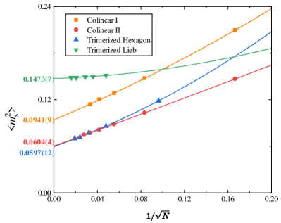
Figure 3: The extrapolation of square staggered magnetization in the four lattices. Error bars are smaller than the size of the symbols. The extrapolated values are shown directly on the horizontal axis using different colors.

It is worth noting that when $g$ falls in the range of $(0,1]$, the ground states of four models exhibit long-range magnetic orders. To assess and compare the relative strengths of magnetic orders in various models, we representatively choose $g=1$ to perform finite-size extrapolations. The order parameter we use for this analysis is the square staggered magnetization, denoted as $m_{s}^{2}$,

$${m_{s}^{2}}=\frac{3}{{{N^{2}}}}{\left|{\sum\limits_{i}{{\phi_{i}}{S_{i}^{z}}}}\right|^{2}},$$ (5)

where the term $\phi_{i}=\pm 1$ represents staggered phase factors, and the factor of three comes from the isotropic strength of all three spin components. To perform the extrapolations, we employ second-order polynomial fittings, the results are presented in Fig. 3. Notably, in the case of $g=1$, where the Collinear I lattice is equivalent to the square lattice, our extrapolated value for $m_{s}^{2}$ aligns well with the results in Ref  [49, 50, 51]. In addition, the trimerized hexagon lattice shares the same diluted configuration as the Collinear II lattice, resulting in nearly the same extrapolated values, as illustrated in Fig. 3. The extrapolated values are shown directly in the horizontal axis of Fig. 3 using different colors.

III.1 Collinear I Lattice

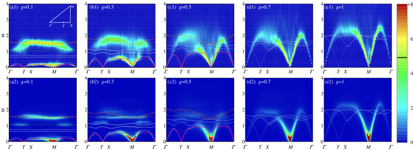
Figure 4: The dynamic spin structure factors of the Collinear I lattice, obtained through QMC and CPT methods, are presented with varying ratios $g=J_{2}/J_{1}$. We follow a high-symmetry path $\Gamma(0,0)$ $\rightarrow$ $T(2\pi/3,0)$ $\rightarrow$ $X(\pi,0)$ $\rightarrow$ $M(\pi,\pi)$ $\rightarrow$ $\Gamma(0,0)$, as shown in the inset of (a1), to show the dynamic spin structure factors. The solid lines indicate the LSWT results of its low-energy effective block spin model. In contrast, the white dotted lines correspond to the LSWT results of the original spin model. The dashed lines in the higher-energy parts denote the well-fitted dispersions which are obtained by the perturbation analysis. Panels (a1)-(d1) display results from QMC-SAC, while panels (a2)-(d2) feature CPT results. For clarity, in the QMC-SAC results, a piecewise function is utilized where the intensity is bifurcated at $U_{0}=5$. When the value is less than 5, the low-intensity section follows a linear distribution. Beyond this threshold, a logarithmic scale is applied, expressed as $U={U_{0}}+{\log_{10}}{S(q,\omega)}-{\log_{10}}{U_{0}}$. However, no additional transformation is applied to the CPT spectrum. This same piecewise function is also used in the subsequent excitation spectra of other lattices.

The first two-dimensional (2D) expansion of trimer blocks we study, termed Collinear I, is depicted in Fig. 1(a1). This structure is a simple expansion of the 1D trimer chain. A main feature of Collinear I is that it can go into the uniform square-lattice Heisenberg model when the ratio $g=J_{2}/J_{1}$ is set to be 1. Fig. 4 shows the dynamic spin structure factors $S(q,\omega)$ changing with $g$. Figures. 4(a1)-(e1) represent QMC-SAC results for various $g$, while Figs. 4(a2)-(e2) display CPT results, corresponding to the same $g$ as used in the QMC-SAC data. This arrangement allows for a direct comparison between two methods under the same $g$ ratio.

From the QMC-SAC data, when $g=0.1$, the doublon band which is approximately at $\omega\approx J_{1}$, and the quarton band which is near $\omega\approx 1.5J_{1}$, start to melt into each other. When $g=0.3$, the doublon and the quarton are highly mixed. As $g$ further increases, the higher part of the excitation spectrum begins to exhibit a continuum near point $X$, and this continuum persists up to $g=1$ which is in the square-lattice Heisenberg limit. In this limit, the broad continuum is due to the deconfined spinon or multimagnon scattering  [52, 53]. For the magnon band, there is gapless Goldstone mode at $M$ and $\Gamma$ points due to the antiferromagnetic ground state. The minimal spectral weight at the $\Gamma$ point is a result of the conservation of total $S^{z}$. With an increase in $g$, both the magnon bandwidth and spin-wave velocity rise. This is accompanied by an elevation of the low-energy magnon spectrum near the point $X$ and a decrease in spectral weights. When $g=0.7$, the low-energy magnon has already merged with the higher-energy part, forming a single magnon mode accompanied by some continuum.

The CPT results exhibit a similar behavior in the low-energy magnon band. However, the doublon and quarton bands are well separated at the smaller $g$ ratios. Regarding the doublon, as the ratio $g$ increases, it becomes more dispersive and eventually forms a dome, becoming a significant part of the single-magnon mode. For the quarton, there appear to be energy splittings with a diminishing spectral weight in the high-energy part and a broadening spectrum near $\omega\approx 1.5J_{1}$. The doublon and quarton eventually merge when $g$ approaches to 1.

The comparison between QMC and CPT in Fig. 4 reveals notable differences in the doublon and quarton bands. The primary distinction lies in the capabilities of each method, as highlighted in Sec. II. The CPT method is exact in the $g\rightarrow 0$ limit. Coupled with the high-accuracy real-frequency dynamics of the ED solver, it can provide detailed information on the dispersions of magnetic quasiparticles for small $g$. In this case, perturbation analysis (PA) works effectively (the details of PA are shown in Sec. IV). The dispersions obtained from PA fit the quarton band of CPT results quite well at small $g$, as can be seen in the orange dashed lines of Fig. 4. The most relevant dispersions are presented in Table. 1 of Sec. IV. However, for larger $g$, the CPT method as a cluster mean-field treatment of magnetic order, can underestimate the quantum fluctuations. Therefore, when the cluster is small, accurately representing the high energy broad continuum becomes challenging. In contrast, QMC with large-scale simulation allows us to obtain a confident spectrum from high-quality imaginary-time Green functions using stochastic analytical continuation (SAC), as demonstrated in Ref. [54]. Regarding the not-so-well separation of doublon and quarton at $g=0.1$, perturbation analysis in Sec. IV also indicates some overlap between the doublon and quarton bands, which we will discuss some more detail later.

As the ground state resides in the Néel phase, we employ the linear spin wave theory to further study the low-energy magnon using two models. The first one is the original spin model on the Collinear I lattice with Néel antiferromagnetic order. Another one is the effective spin-$\frac{1}{2}$ antiferromagnetic model on a rectangle lattice formed by the block spin of each trimer. The effective model has vertical exchange coupling $J_{v}\approx g$ and horizontal coupling $J_{h}\approx\frac{4}{9}g$, as shown in Fig. 8(a), more details about how to get the effective interactions can be seen in Sec. IV. In Fig. 4, the white dotted lines illustrate the LSWT results of the original model, while the pink solid line shows the LSWT results of the effective model. Notably, there is a gapless point at $T(\frac{2}{3}\pi,0)$, which is due to the Brillouin zone folding. When $g$ is small, as depicted in Fig. 4(a1), both the spin wave velocity and the curve of white dotted lines deviate from the magnon band of QMC and CPT. However, the pink solid lines presenting LSWT results of the effective model fit the magnon band well, with better fitting as $g$ decreases. In contrast, as $g$ becomes larger, perturbation analysis becomes less efficient and eventually fails. Therefore, we only present LSWT results of the effective model when $g\leq 0.5$. Due to the stronger ground-state magnetic order, the LSWT results of the original model fit the magnon band increasingly better. At $g=1$, the linear spin wave theory with Oguchi correction  [55] can fit the single magnon mode quite well. This indicates that the LSWT of the original model is a suitable tool for explaining the behavior of the magnon for large $g$ values. However, characterizing the continuum around point $X$ remains challenging within the LSWT framework.

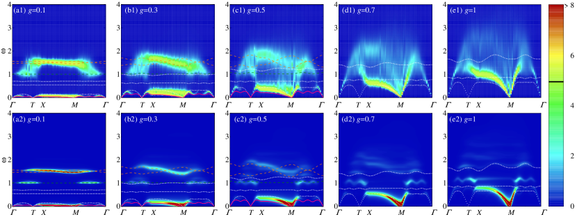
Figure 5: Dynamical spin structure factors of the Collinear II lattice for different $g$ values. The pink solid lines represent the magnon dispersion of the corresponding effective model formed by the trimer block spins, while the white dotted lines illustrate the LSWT results for the original model. The orange and olive dashed lines represent the dispersions of quarton and doublon, respectively, obtained from the perturbation analysis in small $g$. Panels (a1)-(e1) show results obtained from the SAC method, and (a2)-(e2) are the results obtained from the CPT. The high-symmetry path is the same as the Collinear I model as shown in the inset of Fig. 4(a1), and we use the same logarithmic scale in SAC results when $S(q,\omega)>U_{0}=5$, expressed as $U={U_{0}}+{\log_{10}}{S(q,\omega)}-{\log_{10}}{U_{0}}$.

III.2 Collinear II Lattice

In 2015, a research group discovered that CaNi₃(P₂O₇)₂ possesses an internal 2D trimer structure  [22], similar to our second model of interest—Collinear II. Although the nickel ion has a spin quantum number of $S=1$  [56, 57, 58], our study focuses on the $S=1/2$ scenario. The Collinear II lattice, shown in Fig. 1(b1), includes three sites and four connected bonds per trimer. Compared with Collinear I, there is the dilution of vertical bonds along the $y$ direction, suggesting that the continuum observed at larger $g$ values may be a characteristic of trimer chain features [48]. The dynamic spin structure for various $g$ values, alongside effective dispersions and LSWT results, are shown in Fig. 5. The Brillouin zone for Collinear II is identical to that of Collinear I, so the path followed. Similarly, the ground state of this model also resides in the Néel phase.

In Figs. 5(a1)-(e1), the dynamic spin structure factors $S(q,\omega)$ of Collinear II exhibit similarities to Collinear I. Notably, the points at $\Gamma$, $M$ and $T$ are gapless. For $g=0.1$, as seen in Fig.5(a1), the excitation spectrum distinctly separates into magnon, doublon, and quarton parts. The magnon is observed at $\omega<0.144J_{1}$, the doublon around $\omega\approx J_{1}$, and the quarton near $\omega\approx 1.5J_{1}$. In Fig.5(a1), the doublon and quarton are more distinctly separate due to more localized excitations with fewer connection bonds along the $y$ direction compared to Collinear I. It is important to note that while SAC results can depict well-separated doublon and quarton using equal amplitudes $\delta$ functions, the sharpness in the spectral function $S(q,\omega)$ might not accurately represent the true signal. This consideration led us to use variable amplitudes in our sampling process  [41].

As $g$ increases, the few connection bonds along the $y$ direction introduce quasi-1D physics into the dynamic spin structure factors. The non-uniformity of the correlation effect caused by the exchange interaction in the $x$ and $y$ directions becomes increasingly pronounced in the SAC spectrum. In this case, the doublon and quarton mix and melt into each other, and form a broad continuum, while the energy band of the low-energy magnon, continues to expand upwards with the vanishing of the spectrum around point $T$ and eventually becomes the lower bound of the continuum spectrum.

For the CPT results shown in Figs. 5(a2)-(e2), the dispersions of doublon and quarton are revealed in detail when $g\leq 0.3$. The CPT data is utilized in selecting the best fitting curve from perturbation analysis (see Sec. IV), shown with orange dashed lines for quarton and olive dashed lines for doublon. The details of the dispersions are shown in Table.1 of Sec. IV. When $g=0.3$, the spectrum weight of one quarton dispersion is vanishing in the excitation spectrum, as shown in Fig. 5(b2). Due to the limitations of the small cluster used in CPT and the overestimation of magnetic order, the high-energy broad continuum cannot be well characterized. However, the low-energy magnon band closely resembles the QMC results. In Figs. 5(a2)-(e2), we set the broadening factor $\eta=0.01$ for $g=0.1$ and $\eta=0.05$ for other $g$ values.

To analyze the low-energy magnon, we also calculate the LSWT results of the effective model and the original model, shown with dotted white lines and pink solid lines in Fig. 5, respectively. The smaller $g$ is, the better the LSWT of the effective model can fit. The effective model is an antiferromagnetic Heisenberg model on a rectangle lattice with different vertical exchange interaction $J_{v}\approx g/9$ and horizontal interaction $J_{h}\approx 4g/9$, as can be seen in Fig. 8(b) and Sec. IV with more details. When $g=0.1$, the pink solid line aligns closely with the QMC-SAC and CPT results. Particularly in the path from $M$ to $\Gamma$, as depicted in Fig. 5(a1), the pink line accurately matches the ripple-like dispersions observed in the low-energy magnon excitation spectra. However, it is observed that the effectiveness of this effective model diminishes with an increase of $g$. For instance, at $g=0.5$, the pink solid line deviates significantly from the magnon part of QMC-SAC and CPT spectra. This deviation becomes even more pronounced at larger $g$. In contrast, as $g$ increases, the spin wave velocity of the lowest branch obtained by LSWT on the original model tends to the QMC one, although the total dispersion band requires high-order corrections of LSWT. Unfortunately, the high-energy broad continuum cannot be described by the LSWT due to strong quantum fluctuations.

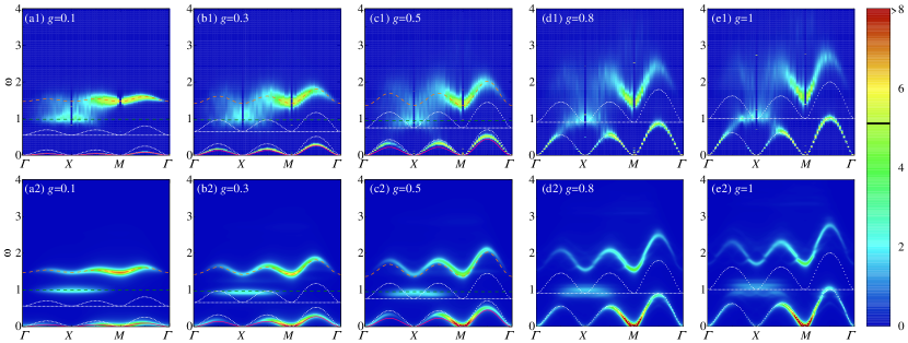
Figure 6: Dynamical spin structure factors of the trimerized Lieb lattice at various $g$ values. The pink solid lines represent the magnon dispersions of the corresponding effective model formed by the trimer block spins. The white dotted lines illustrate the LSWT results of the original model. The orange and olive dashed lines represent the dispersions of quarton and doublon, respectively, obtained from the perturbation analysis in small $g$. Panels (a1)-(e1) show results obtained from the QMC-SAC method, while (a2)-(e2) present results obtained from CPT. The high-symmetry path is shown in the inset of Fig. 4(a1), and we use the same logarithmic scale in QMC-SAC results when $S(q,\omega)>U_{0}=5$, expressed as $U={U_{0}}+{\log_{10}}{S(q,\omega)}-{\log_{10}}{U_{0}}$.

III.3 Trimerized Lieb Lattice

The trimerized Lieb lattice depicted in Fig. 1(c1), is formed by folding the trimer into a perpendicular block and is comprised of three sites and four bonds. This lattice corresponds to a $1/4$-depleted square lattice when $g=1$. The dynamic spin structure factors for this lattice model are presented in Fig. 6. It follows the same Brillouin zone path as that of Collinear I and Collinear II.

In Figs. 6(a1)-(e1), we can discern three distinct energy levels in the QMC calculations. A notable feature is the prominent flat band  [59], positioned at around $\omega\approx J_{1}$. As the $g$ increases, this band slightly decreases and then increases back to around $\omega\approx J_{1}$. The origin of the flat band in trimerized Lieb lattice is similar to the other ferromagnetic lattices, as a consequence of destructive interference between different “hopping” paths of quasiparticles, like doublon.  [60, 61, 62, 63]. Concurrently, the bandwidths of the low-energy magnon and high-energy quarton expand, while the spectral associated with the doublon and quarton around point $X$ becomes broad, indicating the strong scattering between these two quasi-particles. At high symmetry points like $X$ and $M$, there are considerably strong delta peaks at the wrong $\omega$. This is an over-fitting of $S(q,\omega)$, a phenomenon previously observed in the spin-1/2 square-lattice Heisenberg antiferromagnet, as reported by Ref  [54]. When $g=1$, the upper boundary of the magnon aligns with $\omega=J_{1}$ at the middle point from $M$ to $\Gamma$, and the low-energy magnon band closely matches the LSWT prediction on the original model (see white dotted line in Fig. 6 (e1)) without any further correction. This is due to the ferrimagnetic ground state with effective ferromagnetic exchange interaction between trimers which is reflected in the quadratic dispersion at around $\Gamma$, $X$, and $M$. However, the broad continuum and the possible separation of the upper two bands cannot be described by the LSWT of the original model. In addition, when $g$ is small, like $g=0.1$, the LSWT of the effective block spin model with both the same ferromagnetic exchange interaction along $x$ and $y$ directions is more suitable to fit the dispersion of low-energy magnon. The effective interaction strength is $-2g/9$ from our calculation using the Kadanoff method in Sec. IV.

For the CPT results shown in Figs. 6(a2)-(e2), we always observe three separate excitation bands. In the small $g$ regime, the CPT results are more reliable as we mention in Sec. II. We can use perturbation analysis to fit the doublon and quarton bands of CPT results. More details can be found in Sec. IV. These fitting curves (orange dashed lines for quartons and olive dashed lines for doublons) can also match the QMC data quite well. Especially for quarton, the dispersion obtained from perturbation analysis can fit the high energy band quite well even at $g=0.5$. However, due to the limitation of the small cluster, when $g$ gets larger, CPT can overestimate the magnetic order or underestimate the quantum fluctuation, leading to the failure in characterizing the high energy broad continuum around point $X$.

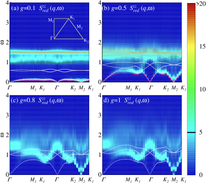
Figure 7: Dynamical spin structure factors in the reduced BZ of the trimerized hexagon lattice at different $g$ values: (a) $g=0.1$, (b) $g=0.5$, (c) $g=0.8$, and (d) $g=1$. The pink lines illustrate the magnon dispersion obtained from LSWT using the low-energy effective block spin model. The white lines represent the LSWT results of the original model. The high-symmetry path is shown in the inset of panel (a), and we use the same logarithmic scale in the SAC results when $S_{red}^{zz}(q,\omega)>5$, expressed as $U={U_{0}}+{\log_{10}}{S_{red}^{zz}(q,\omega)}-{\log_{10}}{U_{0}}$.

III.4 Trimerized Hexagon Lattice

Taking inspiration from the magnetic trimer structure of Ba₄I$r_{3}$O₁₀ as shown in Ref.  [23], the last 2D trimerized lattice we want to study is a trimerized hexagon lattice, illustrated in Fig. 1(d1). Ref  [23] focus on the excitations along the chain direction connected by $J_{2}$, while we are interested in the overall spectra on this hexagon structure. Unlike the honeycomb lattice, its unit cell contains three sublattices instead of two. This lattice is also topologically equivalent to a trimerized square lattice with the same ratio but a different position of bond depletion along the $y$ direction compared to the Collinear II lattice. Consequently, we observe nearly the same antiferromagnetic order in thermodynamic limit for the two lattice models, as shown in Fig. 3. The low-energy effective model for trimer blocks is defined on a rhombus lattice, characterized by bond exchange coupling $J_{v}=J_{h}\approx\frac{4}{9}g$, as can be seen in Fig. 8(d).

Figure. 7 presents the dynamic spin structure factors in the reduced BZ. We illustrated the high-symmetry path in the inset of Fig. 7(a). In the QMC-SAC spectrum at $g=0.1$, the doublon and quarton are distinct. With the increase in $g$, the magnon portion expands, the doublon and quarton quickly mix, and gradually, all three parts merge, presenting a low-energy prominent spin wave and high-energy continuum inherited from the 1D two-spin continuum. The orange and olive lines in Fig. 7(a) and (b) are the dispersions of quarton and doublon, respectively, obtained from the perturbation analysis. At $g=0.5$, olive lines fail to describe the intermediate energy excitation as the doublon and quarton are already mixed into the continuum spectrum. We also display the LSWT results of the original model (dotted white line) and effective model (pink solid line), these two results provide accurate descriptions of low energy magnon in opposite directions of $g$, like their performance in the previous three lattices.

IV Analysis

In the previous section, we have shown some LSWT results of the effective block spin models and some perturbative dispersions for the doublon and quarton. Here in this section, we will give more details about how we get the effective block spin models and do the perturbation analysis for doublon and quarton excitations.

IV.1 Low Energy Effective Models and Magnons

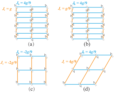
Figure 8: The low-energy effective block spin models of each 2D trimerized lattice when the value $g$ is small. (a) Collinear I, (b) Collinear II, (c) Trimerized Lieb lattice, (d) Trimerized hexagon lattice. The light blue and orange lines represent the effective interactions between trimer blocks along two primitive vectors of unit cells. Here, $J_{h}$ represents an interaction along the horizontal direction of the primitive cell, while $J_{v}$ is associated with the vertical direction. For the trimerized Lieb lattice, the effective interaction is ferromagnetic. $\Uparrow$ represents the effective block spin $S=1/2$ of each trimer. The arrays of $\Uparrow$ and $\Downarrow$ show the magnetically ordered ground state of each effective model.

Due to weak coupling and the effective $S=1/2$ of each trimer in small $g$, we can derive the low-energy effective block spin models of four trimerized systems which will provide more insights into understanding low-energy magnon. Here, we outline the procedures for getting these effective models. Historically, the Kadanoff method has been well developed [64, 65, 66], and used in the studies of quantum criticality both in the low-dimensional and high-dimensional systems [67, 68, 69]. Due to the weak intertrimer interactions and an odd number of spins within a unit cell, an effective spin model can be obtained by projecting the original Hamiltonian onto the effective Hilbert space through the Kadanoff method.

We can formally split the system into the intra-trimer ($H_{\rm{t}}$) and inter-trimer ($H_{\rm{tt}}$) parts which respectively contain the $J_{1}$ and $J_{2}$ couplings. To obtain the effective model, we use the two degenerate ground states of each trimer to construct the basis of the low-energy effective Hilbert space. As shown in Fig. 2, the two degenerate states are given by

$$\left|0\right\rangle^{1/2,-1/2}=\frac{1}{{\sqrt{6}}}\left({\left|{\uparrow\downarrow\downarrow}\right\rangle-2\left|{\downarrow\uparrow\downarrow}\right\rangle+\left|{\downarrow\downarrow\uparrow}\right\rangle}\right),$$ (6)

$$\left|0\right\rangle^{1/2,1/2}=\frac{1}{{\sqrt{6}}}\left({\left|{\downarrow\uparrow\uparrow}\right\rangle-2\left|{\uparrow\downarrow\uparrow}\right\rangle+\left|{\uparrow\uparrow\downarrow}\right\rangle}\right),$$ (7)

where we have changed the quantum numbers to the superscripts for simplicity. The first superscript is the total spin quantum number of a trimer, and the second one is the magnetic quantum number. These two ground states have the opposite magnetic quantum number $\pm 1/2$. We can rename the base kets in the effective Hilbert space, $\Uparrow$ and $\Downarrow$, and construct the projection operator of the $(i,j)th$-trimer,

$$P_{ij}=\left|0\right\rangle^{1/2,1/2}_{ij}\left\langle\Uparrow\right|_{ij}+\left|0\right\rangle^{1/2,-1/2}_{ij}\left\langle\Downarrow\right|_{ij}.$$ (8)

where $(i,j)$ labels the 2D position of a trimer. Then the effective Hamiltonian up to the first-order correction is given by,

$$H_{\rm{eff}}=P^{\dagger}H_{\rm{t}}P+P^{\dagger}H_{\rm{tt}}P,$$ (9)

where $P=\prod_{i,j}P_{ij}$ is the total projection operator. In detail, the effective Pauli operators are obtained firstly,

$$\tilde{\sigma}_{ij}^{\alpha}=\gamma_{ij}P_{ij}^{\dagger}\sigma_{ij}^{\alpha}P_{ij},$$ (10)

where $\gamma_{ij}$ is the coefficient and $\alpha=x,y,z$. Then, inserting these effective Pauli operators into the Eq.(9), we can obtain the effective Hamiltonian Eq.(11) with the effective exchange interactions shown in Fig. 8. It can be found that, for the trimerized Lieb lattice, the effective exchange interaction between block spins is ferromagnetic and homogeneous along two directions, while the two collinear lattices have inhomogeneous effective antiferromagnetic interactions. Consequently, the low-energy effective Hamiltonian for this model can be reformulated to capture these nuanced characteristics

$${H_{\rm{eff}}}={J_{h}}\sum\limits_{i=1}^{N}{{{\tilde{S}}_{i}}\cdot{{\tilde{S}}_{i+1}}}+{J_{v}}\sum\limits_{j=1}^{{N}}{{{\tilde{S}}_{j}}\cdot{{\tilde{S}}_{j+1}}}$$ (11)

As shown in Fig. 8, the effective exchange interaction along the horizontal direction in our models is represented as $J_{h}$, while the effective exchange interaction along the vertical direction is denoted by $J_{v}$. For the trimerized Lieb lattice, the effective interactions along two directions are the same and have negative values which means the ferromagnetic interactions. Based on these effective models, we can do the LSWT to analyze the low-energy magnon. The LSWT results are overlaid on the corresponding excitation spectra, marked with a pink line for clear visualization. Kadanoff method is exact in the $g\rightarrow 0$ limit. We have already seen that the pink solid lines fit the low-energy magnons quite well in small $g$ (for example $g=0.1$) as shown in Figs. 4- 7. But for the Collinear I lattice, the deviation of spin wave velocity comes from the fact that there are more connecting bonds between the trimers, and a smaller $g$ is needed to see a better fitting result.

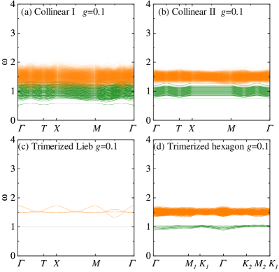
Figure 9: The perturbation dispersion relations for $g$=0.1. (a) Collinear I model, (b) Collinear II model, (c) Trimerized Lieb lattice, (d) Trimerized hexagon lattice. The olive lines denote the doublons and the orange ones denote the quartons.

IV.2 Perturbation Analysis of Doublons and Quartons

Lattice		excitation			dispersions
Collinear I		doublon			$\epsilon=-{E_{0}}+{E_{1}}+7g/9$
					$\epsilon=-{E_{0}}+{E_{1}}+5g/9$
		quarton			$\epsilon=-{E_{0}}+{E_{2}}+4g/9+\sqrt{2}g\cos({3q_{x}})/9+\sqrt{2}g\cos({q_{y}})/3$
					$\epsilon=-{E_{0}}+{E_{2}}+5g/9+g\cos(3{q_{x}})/18+\sqrt{2}g\cos({q_{y}})/3$
					$\epsilon=-{E_{0}}+{E_{2}}+g/9+g\cos(3{q_{x}})/18+\sqrt{2}g\cos({q_{y}})/9$
Collinear II		doublon			$\epsilon=-{E_{0}}+{E_{1}}+g/9+g\cos({q_{x}})/3\sqrt{3}$
		quarton			$\epsilon=-{E_{0}}+{E_{2}}+g/9+g\cos(3{q_{x}})/9+4g\cos({q_{y}})/9$
					$\epsilon=-{E_{0}}+{E_{2}}+g/9-g\cos(3{q_{x}})/6\sqrt{3}-2g\cos({q_{y}})/3\sqrt{3}$
Trimerized Lieb lattice		doublon			$\epsilon=-{E_{0}}+{E_{1}}-2g/9$
		quarton			$\epsilon=-{E_{0}}+{E_{2}}+7g/18-g\cos({2q_{x}})/3-g\cos({2q_{y}})/3$

Table 1: The well-fitted dispersions in the different lattices.

The doublons and quartons in the 2D trimerized models can be conceptualized as propagating internal trimer excitations. In INS experiments and the dynamic spin structure factors, which probe the $S=1$ excitation, we focus on propagating the trimer excitation states where $|\Delta m|=1$ for doublons and $|\Delta S|=1$ for quartons. As depicted in Fig. 2, a transition from the ground state $\left|0\right\rangle^{\frac{1}{2},\frac{1}{2}}$ to the first excited state $\left|1\right\rangle^{\frac{1}{2},-\frac{1}{2}}$ results in a $|\Delta m|=1$ change which are shown by the orange dashed lines, leading to the formation of a doublon. A similar doublon excitation occurs when $\left|0\right\rangle^{\frac{1}{2},-\frac{1}{2}}$ jumps to $\left|1\right\rangle^{\frac{1}{2},\frac{1}{2}}$, as shown by the blue dashed lines. Quartons are more complex, representing the second excitation states with a $|\Delta S|=1$ change, and are shown by solid lines in Fig. 2. That is the excitation from $\left|0\right\rangle^{\frac{1}{2},m}$ to $\left|2\right\rangle^{\frac{3}{2},m^{{}^{\prime}}}$, giving rise to the quartons.

To further analyze the higher energy doublon and quarton excitations in small $g$, we do the perturbation analysis to give some analytical dispersions of these two quasiparticles. By ignoring the entanglement and fluctuation between trimers as a perturbation, the ground-state wave functions of models can be seen as the product states,

$$\left|\psi_{g}\right\rangle=\bigotimes_{i,j}\left|0\right\rangle_{i,j},$$ (12)

where $\left|0\right\rangle_{i,j}$ is the ground state of $(i,j)_{th}$-trimer. For the Collinear I, Collinear II, and trimerized hexagon lattices, their low-energy effective antiferromagnetic interactions between trimer blocks indicate that the true ground states are the total-spin singlets satisfying $m=\sum m_{i,j}=0$. It means that the numbers of $\left|0\right\rangle^{1/2,-1/2}$ and $\left|0\right\rangle^{1/2,1/2}$ should be equal. For the trimerized Lieb lattice, we only choose $\left|0\right\rangle^{1/2,1/2}$ to construct the many-body ground state due to the effective ferromagnetic interaction. In the excited state $\left|\psi\right\rangle_{e}$, we consider one of the $\left|0\right\rangle^{1/2,-1/2}$ and $\left|0\right\rangle^{1/2,1/2}$ is excited following the selection rule as shown in Fig. 2. We can calculate the dispersion relations in the reduced BZ,

$$\epsilon(q) = \left\langle H\right\rangle_{e}-\left\langle H\right\rangle_{g}$$

$$= \left\langle\psi_{e}^{q}\right|H\left|\psi_{e}^{q}\right\rangle-\left\langle\psi_{g}^{q}\right|H\left|\psi_{g}^{q}\right\rangle,$$

where $\left|\psi_{g}^{q}\right\rangle$ and $\left|\psi_{e}^{q}\right\rangle$ are the Fourier transformation of ground state $\left|\psi_{g}\right\rangle$ and excited state $\left|\psi_{e}\right\rangle$, respectively. In practice, we consider random arrangements of the states $\left|0\right\rangle^{1/2,-1/2}$ and $\left|0\right\rangle^{1/2,1/2}$ on each trimer to better mimic the true ground state and extract the optimal dispersion relation. We can conclude that the dispersion relations mainly depend on the excited trimers and their neighbors, only $4\times 4$ trimers are enough to complete the derivation of dispersion relations. This method provides us with more insight to understand the intermediate-energy and high-energy excitations for the four trimerized models, which have been successfully applied in the 1D trimer chain.

When the values of $g$ are small, as shown in Fig. 9, the doublon dispersions are localized near $\omega=J_{1}$, while the quarton dispersions are localized near $1.5J_{1}$. We can also see the bandwidths of the excitation spectra. For the Collinear I lattice at $g=0.1$ in Fig. 9(a), the doublon and quarton excitations seem to have already mixed. That can be used to explain the melting of two parts of the spectrum obtained from QMC-SAC shown in Fig.4(a1). With $g$ increases, the doublon and quarton mix first and then merge with the low-energy magnon into magnon modes or continuum.

We show the well-fitted dispersions by dashed lines in Fig. 4- 6 and show the formula in Table. 1, with orange lines for the quartons and olive lines for the doublons. The coefficients of $cosq_{x}$ and $cosq_{y}$ are positive in Collinear I, Collinear II, and trimerized hexagon lattices, which correspond to the antiferromagnetic ground states. In contrast, the coefficients are negative for the effective model of trimerized Lieb lattice with a ferromagnetic ground state. We find these well-fitted dispersions out of thousands of dispersions. Notably, not all of the dispersions carry significant spectrum weight, and some have only a slight weight. As a result, we selectively focus on a few of them, which can be used to match the CPT and QMC-SAC results closely.

Based on the results from QMC-SAC, CPT, and PA, at small values of $g$, the magnon, doublon, and quarton are in clear distinctions. As $g$ increases, the doublon and quarton begin to mix. However, each method has its limitations. For QMC-SAC, it is hard to see the clear separation of two nearby bands with a narrow band gap. For CPT, the overestimation of magnetic order makes it difficult to describe the high-energy continuum. For PA, it only works for small $g$. Therefore, it is challenging to determine the exact $g$ at which these three excitations start to mix.

V Summary and Discussion

In our study, we explore the evolutions of three types of excitations—magnon, doublon, and quarton for four trimerized Heisenberg models, using a combination of QMC-SAC and CPT methods. In small $g=J_{2}/J_{1}$, we always can see the distinct energy separations of three quasiparticles. As the $g$ increases, the doublon and quarton bands are first to mix to form some continua. Finally, the low-energy magnon and high-energy parts are involved together. For the low-energy magnon, we use linear spin wave theory for both the effective block spin model and the original model to do the analysis. The LSWT of the effective model can fit the magnon curves in the small $g$, while the LSWT of the original model can fit the low-energy magnon part quite well in the large $g$ due to the strong magnetic orders of ground states. Additionally, perturbation analysis is employed to qualitatively assess the behavior of doublons and quartons, particularly at small $g=J_{2}/J_{1}$ values. Our numerical results and analysis provide some universal dynamic behaviors of 2D trimer systems which can help to analyze the inelastic neutron scattering data of some trimer materials in the future.

In real materials, a relatively weak coupling $J_{3}$ often exists between the $a$ and $c$ sublattices  [23]. Due to the sign problem induced by the antiferromagnetic $J_{3}$, we cannot use QMC to obtain the dynamic spin structure. However, we believe that it does not significantly alter the main physics underlying the three types of excitations. In addition, some trimer materials, like CaNi₃(P₂O₇)₂, would have a spin quantum number larger than $1/2$  [56, 57, 58]. For the large spin cases, such as $S=1$ and $S=3/2$, the low-energy spectrum should still be magnon excitation for the 2D case, while the higher energy part is more complex, which is an interesting topic we leave for future study.