An $\ell^{1}$-Plug-and-Play Approach for Magnetic Particle Imaging Using a Zero Shot Denoiser with Validation on the 3D Open MPI Dataset

Abstract

Magnetic particle imaging (MPI) is an emerging medical imaging modality which has gained increasing interest in recent years. Among the benefits of MPI are its high temporal resolution, and that the technique does not expose the specimen to any kind of ionizing radiation. It is based on the non-linear response of magnetic nanoparticles to an applied magnetic field. From the electric signal measured in receive coils, the particle concentration has to be reconstructed. Due to the ill-posedness of the reconstruction problem, various regularization methods have been proposed for reconstruction ranging from early stopping methods, via classical Tikhonov regularization and iterative methods to modern machine learning approaches. In this work, we contribute to the latter class: we propose a plug-and-play approach based on a generic zero-shot denoiser with an $\ell^{1}$-prior. Moreover, we develop parameter selection strategies. Finally, we quantitatively and qualitatively evaluate the proposed algorithmic scheme on the 3D Open MPI data set with different levels of preprocessing.

1 Introduction

Magnetic Particle Imaging (MPI) is an emerging medical imaging modality that images the distribution of superparamagnetic nanoparticles by exploiting their non-linear magnetization response to dynamic magnetic fields. The principles behind MPI have been introduced in the Nature paper by Gleich and Weizenecker [17]. Later, Weizenecker et al. [66] produced a video (3D+time) of a distribution of a clinically approved MRI contrast agent flowing through the beating heart of a mouse, thereby taking an important step towards medical applications of MPI. Further, Gleich, Weizenecker and their team won the European Inventor Award in 2016 for their contributions on MPI. Since then, interest in the technology has been on the rise both with view towards applications and with view towards improving the technology on the hardware side as well as on the algorithmic side.

There are various medical applications such as cancer detection [54] and cancer imaging [15, 58, 69], stem cell tracing [12, 29, 42], inflammation tracing and lung perfusion imaging [71], drug delivery and monitoring [72], cardiovascular [6, 60, 62] and blood flow [16] imaging as well as brain injury detection [46]. MPI can be also used within multimodal imaging [3]. Further applications can be the tracking of medical instruments [25], as well as MPI-assisted stroke detection and brain monitoring based on recent human-sized MPI scanner [20]. Benefits of MPI are quantifyability and high sensitivity, and compared with other imaging modality such as CT [10], MRI [50], PET [59] and SPECT [40], its ability to provide higher spatial resolution in a shorter acquisition time and the absence of ionizing radiation or radioactive tracers [37]. Further details concerning comparison with existing imaging modalities and further examples of state-of-the-art applications can be found in [8, 67].

In brief, the principle and the procedure behind MPI are as follows: (i) the specimen to be scanned is injected with a tracer containing the magnetic nanoparticles (MNs); (ii) a dynamic magnetic field with a low-field volume (LFV) is applied and the LFV is spatially moved; (iii) the LFV acts as a sensitive region whose motion causes the particles to induce a voltage in the receive coils. The imaging task of MPI is the reconstruction of the spatial distribution of the particles in the tracer from the voltage signal acquired during a scan. There are currently two main types of approaches to reconstructing particle distributions: measurement-based approaches and model-based approaches. Measurement-based approaches typically acquire a system matrix: for each column, one performs scanning of a delta probe located in a corresponding voxel of a chosen 3D voxel grid [35, 65, 48, 41]. More precisely, a 3D grid of the volume to be scanned inside the scanner’s bore is considered; a probe with a reference concentration of tracer is iteratively positioned and scanned at each voxel of the grid. This way the response of the scanning system to discrete delta impulses at each voxel position is collected and stored in the system matrix $A.$ Assuming linearity, the acquired signal $f$ of the scan of a specimen is then obtained as a superpositon of the scans of the delta impulses. For reconstruction, one has to solve a corresponding system of equations $Au=f,$ where the symbol $u$ denotes the desired concentration; loosely speaking, one has to invert the system matrix for the measured signal $f$. Due to the presence of noise and the ill-conditioning of the system matrix (e.g., [38, 56]), regularization techniques are needed for the inversion as discussed later. The development of model-based reconstruction techniques is another direction of research aiming at avoiding or significantly reducing the calibration procedures needed for measuring the system matrix; for details, cf. for instance  [47, 51, 18, 19, 21, 45, 9]. In this work we consider the measurement approach and focus on regularized machine-learning based reconstruction in that scenario.

Related Work

Due to the ill-conditioning of the system matrix and the related ill-posedness of the reconstruction problem in MPI [34, 45, 33] small perturbations in the data can lead to significant errors of the reconstruction; thus, regularization is needed [7]. Classical regularization approaches in MPI include Tikhonov regularization [66, 38] using conjugate gradients and the Kaczmarz method. To improve noise suppression capabilities and further features, structural priors based on the $\ell^{1}$-norm have been used within iterative schemes; e.g.[56]. For a broader overview we refer to [13].

In recent years, there is increasing interest in reconstruction methods involving machine learning approaches. Among these are methods learning the reconstruction by directly training a neural network, e.g. [27, 63]. Further, reconstruction based on the Deep Image Prior (DIP) has been proposed [14, 61]. Recently, Deep Equilibrium Models have been employed in the context of MPI [24, 5]. Deep learning approaches have been further used to improve the spatial resolution of the reconstructions [53], and to reduce the calibration time, for example by partially acquiring system matrix on a down-sampled grid and use deep-learning for super-resolution of the system matrix [22, 52, 23, 68].

A particular class of machine learning approaches are plug and play (PnP) approaches. They are inspired by iterative schemes realizing energy minimization: building on an iterative scheme, they replace the denoiser implied by the scheme by an arbitrary one; instead of classical denoising, typically machine-learning based denoisers are employed [70]. PnP approaches have been used for a variety of imaging modalitites, e.g., [2, 55] as well as for computer vision tasks, e.g., [70, 57]. These approaches are conservative in the sense that machine learning only enters the scheme via iterative denoising and that well-known and well-understood components from iterative schemes and classical Tikhonov regularization are still integrated into the reconstruction scheme.

Most closely related to the present work is the paper [4] which also considers a plug and play prior for MPI reconstruction. Our approach differs in the underlying iterative scheme and the denoising method used, which is at the heart of a PnP approach, and in the employment of an additional $\ell^{1}$-prior. We further provide both quantitative and qualitative evaluation on the full 3D Open MPI data set [39]. A detailed discussion concerning the novelties compared to [4] can be found in the discussion in Section 4.1.

Contribution

In this work we develop a plug and play (PnP) approach for MPI reconstruction based on a generic (zero-shot) denoiser, a half quadratic splitting scheme plus an $\ell^{1}$-prior. Moreover, we develop parameter choice strategies, and evaluate the proposed method on the publicly available Open MPI data set. In detail, we make the following contributions:

• In the proposed $\ell^{1}$-PnP method we employ a generic (zero-shot) image denoiser. This means the denoiser is not transfer learned on MPI or similar MRI data. (To apply the 2D image denoiser on a 3D volume, we use slicing.) The approach is inspired by the recent observations in Computer Vision that larger models pretrained on larger training sets perform extremely well even when employed in off-distribution contexts. We further employ a shrinkage/ $\ell^{1}$-prior which is motivated by the works [56, 32] which use a corresponding prior in an energy minimization frameworks in MPI reconstruction.

• We propose parameter selection strategies.

• We quantitatively and qualitatively evaluate our approach on the full 3D Open MPI data set [39] which presently represents the only publicly available real MPI data set. In particular, we quantitatively and qualitatively compare our method with the DIP approach [14] using the preprocessing pipeline [31] and classical Tikhonov regularization. Further, we evaluate the approach with the parameter selection and stopping criteria strategies. Moreover, we investigate the influence of the preprocessing on the reconstruction quality.

Quantitative and qualitative evaluation of a PnP approach (including comparison with another machine learning approach) on the full 3D Open MPI data set has not been done before. (We note that quantitative evaluation is possible on the Open MPI dataset since a reference CAD model is available in the dataset and serves the purpose of a ground truth [39]). Further, employing a zero-shot denoiser [70] (trained on a large set of natural images) is new.

Outline

In Section 2 we develop the method: we describe the formal MPI reconstruction problem (Section 2.1), the preprocessing pipeline of the MPI data (Section 2.2), we present the proposed $\ell^{1}$-PnP approach (Section 2.3), and we consider parameter selection (including a stopping criterion) in Section 2.4. In Section 3 we quantitatively and qualitatively evaluate the proposed $\ell^{1}$-PnP algorithm on the OpenMPI Dataset: we compare with the DIP and Tikhonov regularization (Section 3.3), investigate the influence of different levels of preprocessing (Section 3.4) and consider a setup without preprocessing in Section 3.5. We conclude with Section 4 which contains a discussion and a conclusion part.

2 Method

We first recall the formal problem of MPI reconstruction based on a system matrix approach in Section 2.1. Then we discuss the employed preprocessing in Section 2.2. Finally, we derive the proposed $\ell^{1}$-PnP approach using a zero-shot denoiser in Section 2.3 and consider parameter selection in Section 2.4.

2.1 Reconstruction Problem in MPI Using a System Matrix

The task of MPI reconstruction is to determine the density $u$ of iron oxide nanoparticles contained in an object. We briefly describe the basic principle of a field-free point (FFP) scanner; for details we refer to [37]. A specific static magnetic field is applied to saturate the nanoparticles everywhere in a field of view but in a small region. Such low-field region is a small neighborhood of a point called the Field-Free Point (FFP). A second dynamic magnetic field is applied to steer the FFP in the field of view. The movement of the FFP constitutes a scan: the change of magnetization of the iron oxide particles due to the movement of the FFP induces a voltage in a set of receive coils which constitutes the measured data $f$. The relation between the concentration $u$ and the measured data $f$ is modeled as a linear mapping called the system function or system matrix $A$. In order to determine the system matrix/function both model and measurement-based approaches have been applied; cf. [48, 36] for instance. In real data scenarios, at present, the measurement-based approach is mostly used: the system matrix is obtained by measuring the system response to delta probes centered at all voxel. We consider MPI reconstruction in three dimesional space using real measurement data from the Open MPI dataset [39]. Hence, the reconstructed 3D image/volume $\tilde{u}$ lives in the space $X=\mathbb{R}^{n_{1}\times n_{2}\times n_{3}},$ where $n_{1}=n_{2}=n_{3}=19$ for the Open MPI data set. We denote the total number of voxels by $N=n_{1}n_{2}n_{3}=19^{3},$ and the number of measurements by $M$; here $M$ depends on the preprocessing applied to the MPI data (cf. Section 2.2). In particular, a scan in the Open MPI dataset contains the data coming from three different channels and the calibration data is Fourier transformed. This means that for each of the three channels the real and imaginary parts of the Fourier coefficients are considered and stacked, yielding a real-valued submatrix $A_{l}$. Finally, the full matrix $A$ is formed by stacking the submatrices $A_{l}$ for each channel $l$ (for a detailed explanation we refer the interested reader to [31]). In order to avoid notation issues, we use the following conventions: we use the symbol $u\in\mathbb{R}^{N}$ to denote the (columnwise) vectorization of the volume $\tilde{u}\in\mathbb{R}^{n_{1}\times n_{2}\times n_{3}}.$ We then identify the system matrix with a matrix $\tilde{A}\in\mathbb{R}^{M\times N}$ such that $\tilde{A}\tilde{u}=Au$ for all volumes $\tilde{u}\in\mathbb{R}^{n_{1}\times n_{2}\times n_{3}}$. We further identify the adjoint $A^{\ast}$ of $A$ with the matrix $\tilde{A}^{T}$; in particular, for any $g\in\mathbb{R}^{M},$ we have that $A^{\ast}g$ equals the reshape operation (which inverts the vectorization operation) of $\tilde{A}^{T}g$. Using this notation, we have the relation

$$f=Au+\eta=\tilde{A}\tilde{u}+\eta.$$ (1)

where $\tilde{A}\in\mathbb{R}^{M\times N}$ denotes the system matrix, $u$ denotes the discrete nano-particle density/volume, $f$ the measured data, and the symbol $\eta$ denotes the noise on the measurements. In particular, the $N=19^{3}$ columns of $\tilde{A}$ are obtained by measuring the scanner’s response to delta probes sitting in the respective voxels. The reconstruction task consists of determining $u$ in Eq. (1) given measurements $f$ (and $A$). This is challenging due to noise and the ill-conditioning of $A$ and requires regularization as already discussed.

2.2 Preprocessing of MPI Data

We briefly discuss the preprocessing of the Open MPI data employed. It is inspired but not identical to the preprocessing proposed of [31]. For this reason, and since we discuss our scheme w.r.t. different levels of preprocessing in the experimental section, we briefly explain the used method.

Preprocessing is applied to both calibration and phantom scan data. Since the calibration data are stored in the Fourier domain we transform the scan data (given as a time series) to the Fourier domain. We further split the real and imaginary part of the Fourier coefficients for both calibration and phantom data. Although any preprocessing step may decrease the number of rows of $A,$ we always use the same symbol $M$ to denote these numbers.

Bandpass Filtering and Frequency Selection

Due to analog filtering, the measurement data show a very high variance in the frequencies up to 75kHz. We therefore exclude frequencies lower than 80kHz. Further frequency selection avoiding frequencies with systematic strong noise or with low signal-to-noise ratio (SNR) has been considered in [31]. To reduce the number of variables at play and to avoid estimations of the SNR we consider no SNR-based thresholding in the preprocessing here.

Background Correction

The noisy measured phantom data $f$ is of the form $f=f_{\mathrm{cl.}}+b_{f}+\eta_{f}$, with clean signal $f_{\mathrm{cl.}}$ containing the information on $u,$ the background signal $b_{f}$ produced by the drive field and perturbations in the measurement chain, and noise $\eta_{f}.$ Accordingly, we decompose the system matrix as $A=A_{\mathrm{cl}}+b_{A}+\eta_{A},$ with clean signals $A_{\mathrm{cl}},$ background $b_{A}$ and noise $\eta_{A}.$ To exclude the background signals $b_{f},$ $b_{A}$, background measurements with no phantom in the scanner are performed after the scan and during the calibration procedure. To account for the background signal to be dynamic, it is repeated after every $19$th delta probe scan (after running through the $x$-axis) and a corresponding convex combination is subtracted. Each phantom and delta scan is performed $1000$ times and the average is taken as input for the reconstruction. (By linearity, the averaging and subtraction is in fact carried out in the Fourier domain.) For a more precise description we refer to the Sec. S1 in the supplementary material.

Whitening Estimation and Low Rank Approximation of the System Matrix

Following [14] we consider a whitening matrix $W$ obtained from the diagonal covariance matrix of multiple background scans, i.e., we consider the diagonal matrix $W\in\mathbb{R}^{M\times M}$ whose diagonal entries are $1/\sigma_{b}$ where $\sigma_{b}^{2}$ is the variance of the background scans provided. When whitening is applied, we consider the whitened system matrix $WA$ and the whitened data $Wf$ instead of $A,$ $f$.

The low rank approximation is obtained by selecting $K\leq\min\{M,N\}$ and by performing a randomized Singular Value Decomposition (rSVD) [31, 26], yielding $(\tilde{U}_{K},\tilde{\Sigma}_{K},\tilde{V}_{K})$ and considering for the reconstruction the transformed matrix $\tilde{U}_{K}^{\ast}A\in\mathbb{R}^{K\times N}$ and the transformed data $\tilde{f}=\tilde{U}_{K}^{\ast}f\in\mathbb{R}^{K}$. Because we aim at using the rSVD obtained we store $\tilde{V}_{K}$ and $\mathrm{diag}(\tilde{\Sigma}_{K})\in\mathbb{R}^{K}$ in place of $\tilde{U}_{K}^{\ast}A$.

2.3 The Proposed Plug-and-Play Approach with a Zero-Shot Denoiser

We now describe the proposed $\ell^{1}$-PnP approach. The regularized inversion of the ill-posed MPI reconstruction problem in Eq. (1) can be formulated as a minimization problem of the form

$$\hat{u}=\arg\min_{u}\lVert f-Au\rVert_{2}^{2}+\lambda\mathcal{R}(u),$$ (2)

where $\mathcal{R}$ is a regularizer and $\lambda>0$ is a parameter controlling the strength of the regularization. In the context of MPI, adding positivity and sparsity constraints has turned out to be effective [56, 32]. Adding positivity and sparsity contrains results in a minimization problem of the form

$$\hat{u}=\arg\min_{u}\lVert f-Au\rVert_{2}^{2}+\lambda\mathcal{R}(u)+\alpha\lVert u\rVert_{1}+\iota_{+}(u),$$ (3)

where $\iota_{+}$ is the indicator function defined as $\iota_{+}(u)=0$ if the components $u_{i}$ of $u$ are all $u_{i}>0$ and $\iota_{+}(u)=+\infty$ otherwise.

The Iterative Scheme

Choosing auxiliary variables $u_{1}$, $u_{2}$ and $u_{3}$ we decouple the quantities in Eq. (3), in particular, we choose the following equivalent constrained minimization problem in consensus form:

$$\min_{u_{1},u_{2},u_{3}}\quad \underbrace{\lVert f-Au_{1}\rVert_{2}^{2}+\lambda\mathcal{R}(u_{2})+\alpha\lVert u_{3}\rVert_{1}+\iota_{+}(u_{2})}_{=:E(u_{1},u_{2},u_{3})}$$ (4)

s.t. $$u_{1}-u_{2}=0\quad\text{and}\quad u_{1}-u_{3}=0.$$ (5)

We now perform a Half Quadratic Splitting (HQS) by considering the Lagrangian of the following form $\mathcal{L}_{\mu}(u_{1},u_{2},u_{3})=E(u_{1},u_{2},u_{3})+\frac{\mu}{2}\lVert u_{1}-u_{2}\rVert_{2}^{2}+\frac{\mu}{2}\lVert u_{1}-u_{3}\rVert_{2}^{2}$ with parameter $\mu$. The HQS here chosen in its scaled dual form yields the following iterative scheme:

$$u_{1}^{k+1} =\arg\min_{u_{1}}\lVert f-Au_{1}\rVert_{2}^{2}+\mu_{k}\left\lVert u_{1}-\frac{u_{2}^{k}+u_{3}^{k}}{2}\right\rVert_{2}^{2}$$ (6)

$$u_{2}^{k+1} =\arg\min_{u_{2}}\frac{1}{2(\lambda/\mu_{k})}\rVert u_{2}-u_{1}^{k+1}\rVert^{2}+\mathcal{R}(u_{2})+\iota_{+}(u_{2})$$ (7)

$$u_{3}^{k+1} =\arg\min_{u_{3}}\frac{\alpha}{\mu_{k}}\lVert u_{3}\rVert_{1}+\frac{1}{2}\lVert u_{1}^{k+1}-u_{3}\rVert_{2}^{2}.$$ (8)

In each iteration $k$, the term in Eq. (6) is in charge of the reconstruction whereas the term in Eq. (7) performs regularized Gaussian denoising with positivity constraint. Finally, the term in Eq. (8) is the proximal mapping of the $L^{1}$ norm, i.e., it results in a soft-thresholding.

The Denoising Step

The idea behind the PnP approach is to substitute the Gaussian denoising in Eq. (7) by any other denoiser with positive output and w.r.t. noise level $\lambda/\mu_{k}$, yielding the following algorithm:

$$u_{1}^{k+1} =\arg\min_{u_{1}}\lVert f-Au\rVert_{2}^{2}+\mu_{k}\left\lVert u_{1}-\frac{u_{2}^{k}+u_{3}^{k}}{2}\right\rVert_{2}^{2}$$ (9)

$$u_{2}^{k+1} =\mathrm{Denoiser}\left(u_{1}^{k+1}\,,\sqrt{\lambda/\mu_{k}}\right)$$ (10)

$$u_{3}^{k+1} =\mathrm{prox}_{\frac{\alpha}{\mu_{k}}\lVert\bullet\rVert_{1}}(u_{1}^{k+1}).$$ (11)

The choice of a suitable denoiser in Eq. (10) is key because the performance of the algorithm significantly depends on it. In Computer Vision, machine learning based 2D denoisers have gained a lot of interest in recent years. They are typically trained on large datasets, and possess a higher generalization ability than smaller models.

The denoiser we employ in this work is the benchmark deep denoiser prior [70]. It is based on a deep CNN architecture (DRUNet) which combines a U-Net [49] and ResNet [28]. The denoiser is publicly available and trained on a large dataset that combines various datasets including BSD [11], Waterloo Exploration Database [44], DIV2K [1] and Flick2K [43]. We do not retrain the denoiser on MPI or MPI related data, but employ it as a zero-shot denoiser (in the sense that it has not seen the domain before.)

We perform the denoising of the 3D target in a slicewise fashion strategy [4], i.e., at each iteration $k$ we consider the 2D slices perpendicular to an axis and perform the denoising of each 2D slice with the 2D denoiser. This slicewise denoising is perform at $k$ along each axis and the three resulting volumes are averaged.

The overall algorithm is given in Algorithm 1.

Algorithm 1 The proposed $\ell^{1}$-PnP algorithm.

Input: scan data $f$ and system matrix $A$, parameters $\alpha$, $\mathrm{toll}_{\sigma}$, $\mu_{0}$.
Output: reconstructed volume $u$.

$u_{2}^{0},u_{3}^{0}\leftarrow 0$;

$k\leftarrow 0$;

while $\sigma_{\mathrm{res}}>\mathrm{toll}_{\sigma}$ do

     $u_{1}^{k+1}\leftarrow$ConjGrad$\left(A^{\ast}A+\mu_{k}\mathrm{Id}\,,A^{\ast}f+\mu_{k}\frac{u_{2}^{k}+u_{3}^{k}}{2}\right)$;

     $\sigma_{k}\leftarrow\sqrt{\mathrm{Var}(u_{1}^{k+1})}$;

     if $k=0$ then

         $\lambda\leftarrow\mu_{0}\cdot\sigma_{0}^{2}$

     end if

     $u_{2}^{k+1}\leftarrow$Slicewise-Denoise$\left(u_{1}^{k+1}\,,\sigma_{k}\right)$;

     $u_{3}^{k+1}\leftarrow$Soft-Threshold$\left(u_{1}^{k+1}\,,\frac{\alpha}{\mu_{k}}\right)$;

     $\sigma_{\mathrm{res}}\leftarrow|\sigma_{k}-\sigma_{k-1}\rvert$;

     $\mu_{k+1}\leftarrow\lambda/\sigma_{k}^{2}$;

     $k\leftarrow k+1$;

end while

return $u_{2}^{k+1}$

2.4 Parameter Selection Strategies

The $\ell^{1}$-PnP approach proposed depends on the (hyper) parameters $\mu_{k}$, $\lambda$ and $\alpha$ as well as on the number of iterations $k$ of the scheme (stopping criterium). (Note that the $\sigma_{k}$ are not free parameters, but related via $\sigma_{k}=\sqrt{\lambda/\mu_{k}}$.) Typically, in PnP approaches (e.g., [70]) the corresponding parameters are set fixed, in particular the noise related parameter $\sigma_{k}$ fed into the denoiser is set fixed for each iteration $k$ for a fixed number of iterations. We now propose more adaptive ways to choose the above parameters.

Choice of $\lambda$ and of the $\mu_{k}$

We start out from the relation $\sigma_{k}^{2}=\lambda/\mu_{k},$ noting that the $\sigma_{k}$ have an interpretation as (Gaussian) noise levels of the $u_{1}^{k}$. Using this interpretation, we let

$$\tilde{\sigma}_{k}^{2}=\mathrm{Var}(u_{1}^{k})=\mathbb{E}\left[(u_{1}^{k}-\bar{u}_{1}^{k})^{2}\right],$$ (12)

where $\bar{u}_{1}^{k}$ is the mean of the vector $u_{1}^{k}$. The value $\tilde{\sigma}_{k}^{2}$ is an upper bound on the noise level (and potentially can be seen as a very coarse estimate which empirically turns out to be sufficient for our purposes; another interpretation can be as a normalization.) Then, we set the $\mu_{k}$ by

$$\mu_{k}=\tilde{\mu}_{k}=\tilde{\lambda}/\tilde{\sigma}_{k}^{2}.$$ (13)

To determine $\lambda=\tilde{\lambda},$ we use the relation $\tilde{\lambda}=\tilde{\mu}_{0}\tilde{\sigma}_{0}^{2},$ where we define $\tilde{\sigma}_{0}^{2}$ via Eq. (12), and $\tilde{\mu}_{0}$ by the following observation: initializing $u_{2}^{0}=u_{3}^{0}=0$ in Alg. 1, $u_{1}^{0}$ is the solution of the Tikhonov regularization problem (cf. Eq. (9) and Eq. (2) with $\mathcal{R}(u)=\lVert u\rVert_{2}^{2}$). Consequently, one can set the parameter $\mu_{0}$ to

$$\tilde{\lambda}=\tilde{\mu}_{0}\tilde{\sigma}_{0}^{2},\qquad\tilde{\mu}_{0}=\tilde{\lambda}_{\mathrm{Tik}}$$ (14)

where $\tilde{\lambda}_{\mathrm{Tik}}$ denotes an estimate on the parameter $\lambda_{\mathrm{Tik}}$ of the corresponding Tikhonov problem. Viewing Tikhonov regularization as acting on the singular values of the system matrix $A$ we relate $\tilde{\lambda}_{\mathrm{Tik}}$ to the singular values of $A;$ concretely, we here consider (potentially rough estimates) of the smallest singular value $\sigma_{\mathrm{min}}$ and choose $\tilde{\mu}_{0}$ according to the simple criterion $\tilde{\mu}_{0}=\tilde{\lambda}_{\mathrm{Tik}}=100\,\sigma_{\mathrm{min}}^{2}$ to reduce the impact of the small singular values.

Choice of $\alpha$

In each iteration a soft-thresholding (proximal mapping of the $\ell^{1}$ norm) of parameter $\alpha/\mu_{k}$ is performed (cf. Eq. (11)), and thus all values of magnitude below $\alpha/\mu_{k}$ are set to zero. So, if $c_{\mathrm{rec}}$ is the maximum concentration of the reconstruction, it is necessary that $\alpha<c_{\mathrm{rec}}\cdot\mu_{0}$ not to get the all zeros reconstruction. Therefore, it is reasonable to choose $\alpha$ as some percentage of $c_{\mathrm{rec}}\mu_{0}$. In the Open MPI data set $c_{\mathrm{rec}}\leq 1$, hence $\alpha$ can be though as a percentage of $\mu_{0}$. We refer the interested reader to the Section S4 of the supplementary material for the details. In this work we have set $\alpha=0.005\mu_{0}$ for all experiments.

Stopping Criterion

We propose to consider the increments of the estimated $\tilde{\sigma}_{k}$ in (12), and to stop the iteration when they fall under a fixed tolerance level $\mathrm{tol}_{\sigma},$ i.e., when $\sigma_{\mathrm{res}}^{k}=\lvert\ \tilde{\sigma}_{k}-\tilde{\sigma}_{k-1}\rvert<\mathrm{tol}_{\sigma}$. In this work we have set $\mathrm{tol}_{\sigma}=10^{-4}$ for all experiments.

3 Results

In this section we quantitatively and qualitatively evaluate the $\ell^{1}$-PnP algorithm proposed in Section 2.3 on the OpenMPI Dataset [39]. Qualitative comparision using the well established quality measures PSNR and SSIM is possible by inferring the groundtruth from a CAD model; details are given in Section 3.1. We compare the proposed $\ell^{1}$-PnP scheme with the Deep Image Prior (DIP) and with the standard Tikhonov $\ell^{2}$-regularization as a baseline; these methods are discribed in Section 3.2. The evaluation is conducted in Section 3.3. In particular, in Experiment 1 we compare the results obtained with the DIP and Tikhonov regularization on the 3D Open MPI Dataset using typical preprocessing. In Experiment 2 we investigate the influence of increasingly lower levels of preprocessing. Finally, in Experiment 3 we show the results obtained with $\ell^{1}$-PnP approach without preprocessing using our parameter selection and stopping strategy (and without relying on a SVD).

The preprocessing was implemented in Matlab and the $\ell^{1}$-PnP algorithm in Python 3.9, using Numpy and PyTorch. The experiments were performed on a workstation with 13th Gen Intel(R) Core (TM) i9-13900KS, 128 GB of RAM, an NVIDIA RTX A6000 GPU and Windows 11 Pro.

3.1 Image Quality Measures

In order to quantitatively assess the reconstruction quality, the Open MPI Dataset provides CAD models of the phantoms. This allows to compare the reconstructions with the corresponding ground truth implied by the CAD model. We use both Peak Signal-to-Noise Ratio (PSNR) and the Structural Similarity Index Measure (SSIM) as measures. For details on the employed implementation, we refer to Sec. S2 in the supplementary material.

Since there might be deviations between the position of the scanned phantom and the reference CAD model $u_{\mathrm{ref}}$, we follow [32] and consider the quantity:

$$\mathrm{PSNR}(u)=\mathrm{PSNR}_{\mathrm{max}}(u)=\max_{\Delta r\in\mathcal{R}}\mathrm{PSNR}(u,u_{\mathrm{ref},\Delta r}),$$ (15)

where $\mathcal{R}$ is the set of all reference volumes $u_{\mathrm{ref},\Delta r}$ obtained by considering shifts $\Delta r$ of step size $0.5$mm in the neighborhood $[-3\,\mathrm{mm}\,,3\,\mathrm{mm}]^{3}$. Analogously, we consider the positional-uncertainty-aware measure $\mathrm{SSIM}_{\mathrm{max}}$ as:

$$\mathrm{SSIM}(u)=\mathrm{SSIM}_{\mathrm{max}}(u)=\max_{\Delta r\in\mathcal{R}}\mathrm{SSIM}(u,u_{\mathrm{ref},\Delta r}).$$ (16)

In what follows we always display $\mathrm{PSNR}_{\mathrm{max}}$ and $\mathrm{SSIM}_{\mathrm{max}}$ but stick to the notation PSNR and SSIM for simplicity.

3.2 Methods for Comparison

(Classical) Tikhonov Regularization

The inversion of the system matrix is performed considering the minimization problem in Eq. (2) with $\mathcal{R}(u)=\lVert u\rVert_{2}^{2}$; the minimizer is then obtained solving the associated Euler-Lagrange equations using the Conjugated Gradient (CG) method when the SVD. When available, we use the rSVD of the preprocessing to show that the method works, it is however not necessary and we point this out in Experiment 3.

Deep Image Prior (DIP)

The DIP has been used in MPI [14]. It is, to our knowledge, the only machine learning approach which has been qualitatively and quantitatively evaluated on the Open MPI dataset. It is based on the idea to drop the explicit regularizer $\mathcal{R}$ in Eq. (2) and to use the implicit prior captured by a neural network parametrization, i.e., if $\varphi_{\theta}$ is a neural network with parameters $\theta$ taking as input a noisy array $z$, we can train the network $\varphi_{\theta}$ by solving the following minimization problem

$$\theta^{*}=\arg\min_{\theta}\lVert A\varphi_{\theta}(z)-f\rVert_{p}^{p},$$ (17)

to obtain a reconstruction $u=\varphi_{\theta^{\ast}}(z)$. For details on our implementation we refer to Sec. S3 in the supplementary material.

3.3 Experiment 1: Comparison on the OpenMPI Dataset

The OpenMPI Dataset [39] contains three phantoms designed to offer different challenges for the reconstruction: the shape phantom, the resolution phantom and the concentration phantom. We present both quantitative and qualitative results organized along the phantoms.

Preprocessing

The scan data in this first experiment has been preprocessed as described in Section 2.2, considering frequencies between $80$ and $625$ kHz, with whitening and the low-rank approximation with the rSVD and rank $K=2000$ (as in [14]).

Comparision Methods

We display results for the proposed $\ell^{1}$-PnP approach and the DIP as well as the Tikhonov regularization method. For the comparison method of Tikhonov regularization, we have chosen its parameter $\lambda_{\mathrm{Tik}}$ optimally in the sense that we have performed a grid search and selected that value for which the $\mathrm{PSNR}_{\mathrm{max}}$ is maximal. The grid search proceeds as follows: we first perform reconstruction with parameters $10^{j}$ for $j=1,\cdots,10$ and consider $j^{\ast}$ the exponent that maximizes the PSNR; then we consider the values from $10^{j^{\ast}-1}$ to $10^{j^{\ast}+1}$ with step $10^{j^{\ast}-1}$ and again select the one maximizing PSNR. For the fine-tuning of the DIP comparison method, we have followed the approach proposed in [14]: we let the DIP run for 20000 iterations with three different gradient descent step sizes $\alpha_{i}=10^{-i}$ and we select the reconstruction corresponding to the parameter $\alpha_{i}$ and the iteration $s$ for which $\mathrm{PSNR}_{\mathrm{max}}$ is maximized (we refer to the Section S3 of the supplementary material for a detailed description of the architecture and the parameters we employ here). The optimal Tikhonov parameters and the iterations $s$ corresponding to the best $\mathrm{PSNR}_{\mathrm{max}}$ in the DIP are displayed in Tab. 1.

Parameters for the $\ell^{1}$-PnP Method

We choose the parameters $\mu_{k}$, $k\geq 1,$ $\lambda$ and $\alpha$ as well as the number of iterations $k$ as suggested in Sec 2.4. For $\mu_{0}$ however, we choose the optimal parameter $\lambda_{\mathrm{Tik}}$ computed for the comparison method above (cf. Tab. 1) instead of the estimate $\tilde{\lambda}_{\mathrm{Tik}}$ (cf. (14)). We note that $\lambda_{\mathrm{Tik}}$ is optimized w.r.t. PSNR involving the ground truth. We point out that we display the result upon convergence and do not consider an optimization on the iterations (as we do for the DIP).

Table 1: Concerning Experiment 1, we report the optimal Tikhonov parameters $\lambda_{\mathrm{Tik}},$ the number $s$ of the iteration with maximal PSNR for the DIP for the different gradient steps sizes $\alpha_{i}=10^{-i}$, $i=3,4,5,$ and the number $s$ of iterations of the $\ell^{1}$-PnP implied by the stopping criterion.

Phantom	Method
	Tikhonov	DIP, $\alpha_{3}$	DIP, $\alpha_{4}$	DIP, $\alpha_{5}$	PnP
Shape Ph.	$\lambda_{\mathrm{Tik.}}=23000$	s=110	s=250	s=1900	s=8
Res. Ph.	$\lambda_{\mathrm{Tik.}}=8000$	s=4000	s=1900	s=3000	s=6
Conc. Ph.	$\lambda_{\mathrm{Tik.}}=600$	s=4000	s=3000	s=15000	s=4

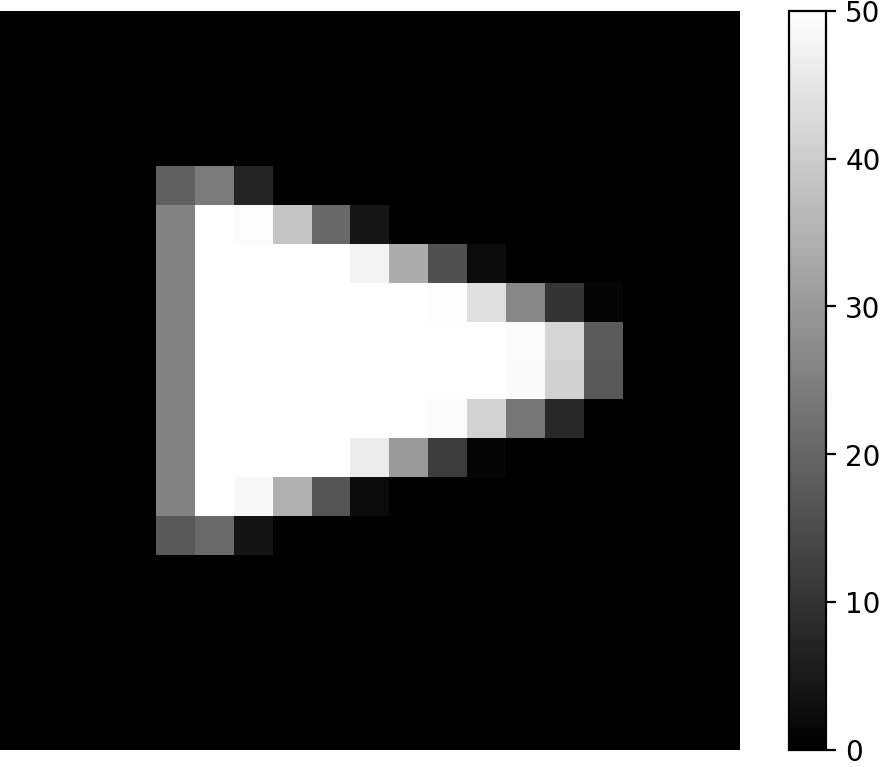
(a) Shape $\rho_{\text{GT}}$.

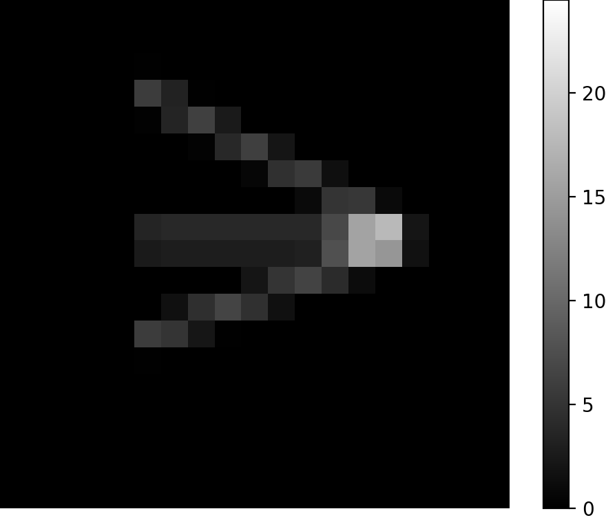
(b) Res. $\rho_{\text{GT}}$.

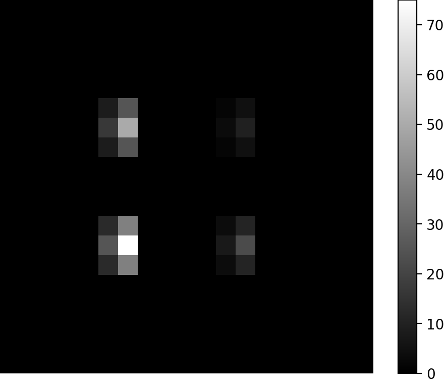
(c) Conc. $\rho_{\text{GT}}$.

(d) Shape $\rho_{\text{Tik}}$.

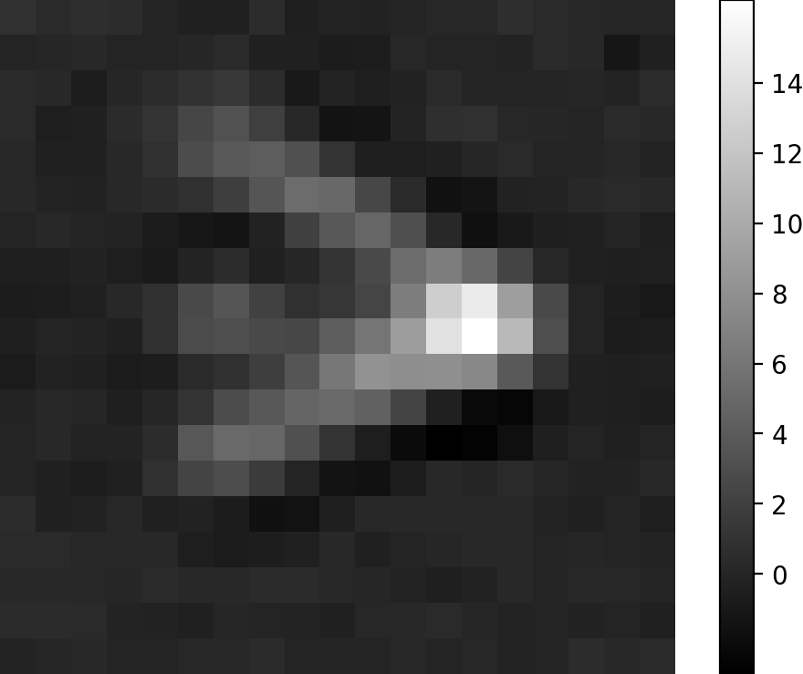
(e) Res. $\rho_{\text{Tik}}$.

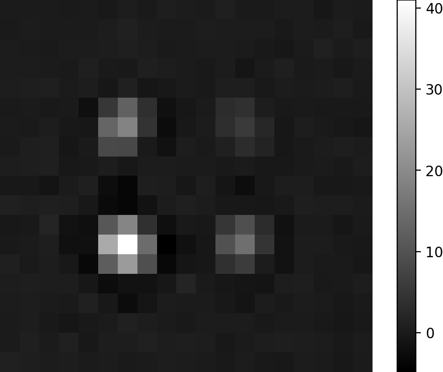
(f) Conc. $\rho_{\text{Tik}}$.

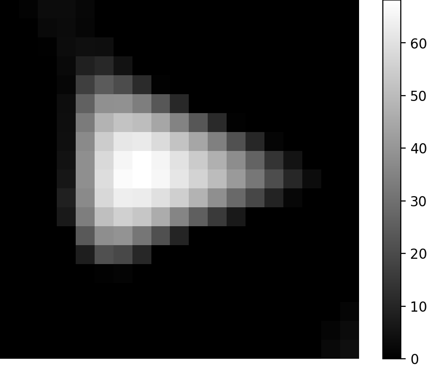
(g) Shape $\rho_{\text{DIP}}$ with $\alpha_{3}$.

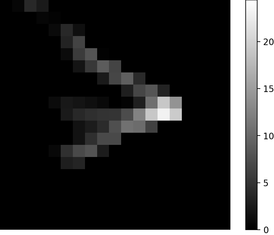
(h) Res. $\rho_{\text{DIP}}$ with $\alpha_{3}$.

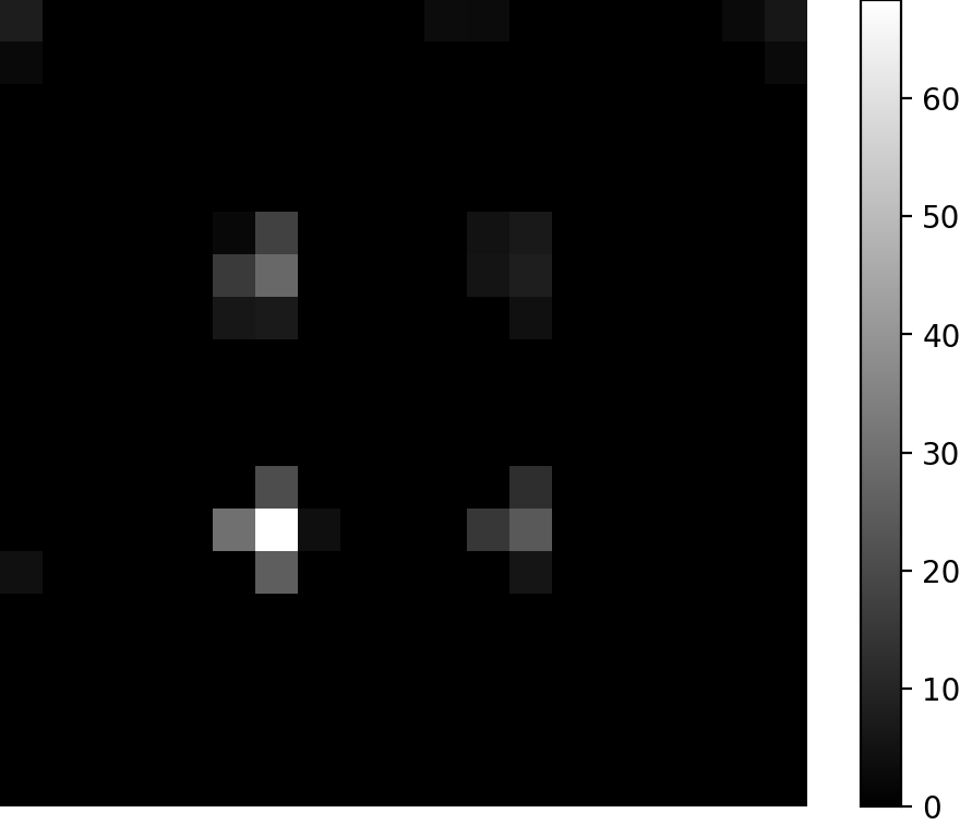
(i) Conc. $\rho_{\text{DIP}}$ with $\alpha_{5}$.

(j) Shape $\rho_{\text{PnP}}$.

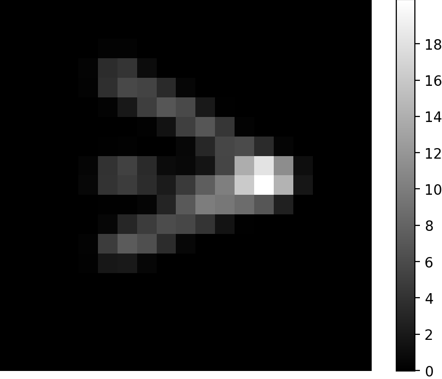
(k) Res. $\rho_{\text{PnP}}$.

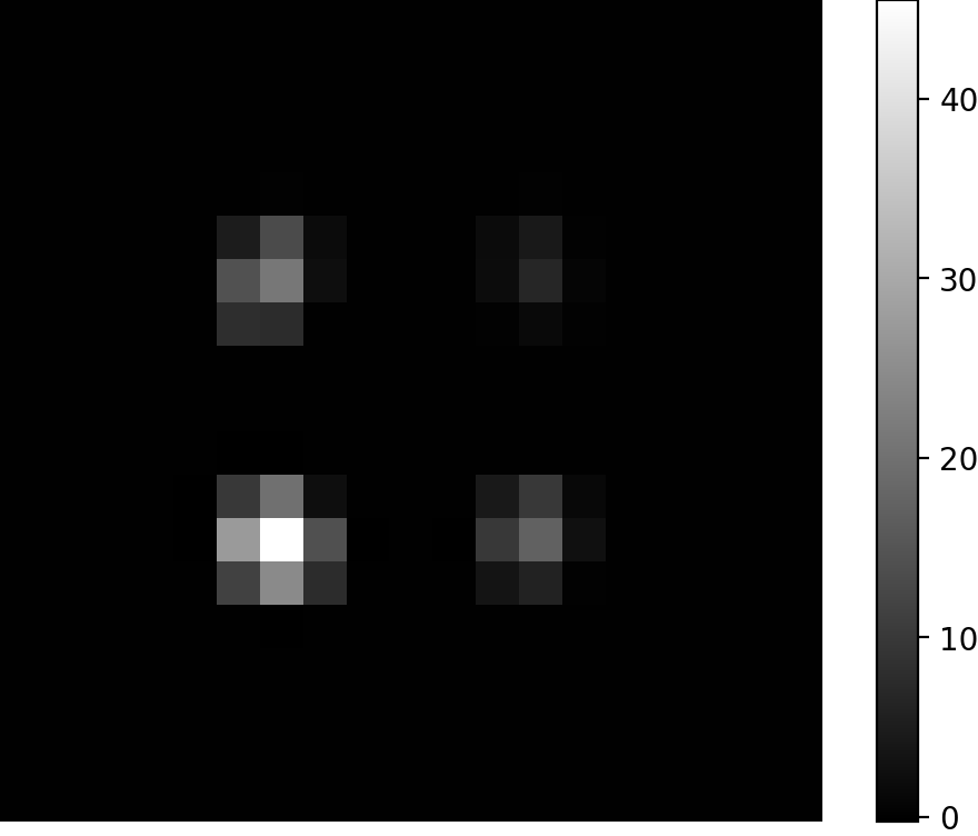
(l) Conc. $\rho_{\text{PnP}}$.

Fig. 1: Selected slices for the Tikhonov reconstruction, the DIP with the $\alpha_{i}$ with the highest PSNR levels and the PnP (cf. Tab. 2). For the shape phantom we display the 10-th xz-slice, for the resolution phantom the 10-th xy-slice and for the concentration phantom the 13-th xy-slice.

Results

Selected slices of the reconstructions are displayed in Fig. 1, we refer the interested reader to the supplementary material (Section S6) for a full display of all slices of the reconstructions.

Table 2: Results obtained with the $\ell^{1}$-PnP, the Tikhonov and DIP methods on the 3D Open MPI data set. We display the PSNR and SSIM scores for the reconstruction obtained maximizing with respect to PSNR for the Tikhonov method. For the DIP with different gradient steps sizes $\alpha=10^{-i}$, $i=3,4,5$ and the $\ell^{1}$-PnP we consider the reconstruction corresponding to the iteration for which the PSNR is maximal. In the last column, we display the results obtained with the $\ell^{1}$-PnP with parameter $\mu_{0}=\lambda_{\mathrm{Tik}}$ chosen as the optimal Tikhonov parameter and the other parameters according to Section 2.4.

Phantom	Metric	Method
		Tikhonov	DIP, $\alpha=10^{-3}$	DIP, $\alpha=10^{-4}$	DIP, $\alpha=10^{-5}$	$\ell^{1}$-PnP (our)
Shape	$\mathrm{PSNR}$	23.06	25.77	22.84	20.07	31.16
Phantom	$\mathrm{SSIM}$	0.505	0.852	0.668	0.508	0.951
Resolution	$\mathrm{PSNR}$	30.32	31.72	31.24	29.43	31.94
Phantom	$\mathrm{SSIM}$	0.505	0.702	0.606	0.432	0.730
Concentr.	$\mathrm{PSNR}$	36.54	37.74	37.65	38.3	37.87
Phantom	$\mathrm{SSIM}$	0.546	0.464	0.508	0.504	0.576

An overview of the results obtained in terms of $\mathrm{PSNR}_{\mathrm{max}}$ and $\mathrm{SSIM}_{\mathrm{max}}$ are displayed in Tab. 2. The $\ell^{1}$-PnP method obtains higher SSIM for all phantoms whereas the PSNR score of the $\ell^{1}$-PnP is significantly higher for the shape phantom, higher for the resolution phantom and lower but comparable for the concentration phantom.

Fig. 2: Example of a profile cut for the shape phantom. We consider the 9-th xz-slice and the cut along the 9-th x pixel.

Because the $19\times 19\times 19$ resolution of the reconstructions, the visual quality assessment of the differences between reconstructions can be difficult. For a better understanding of the differences we have plotted in Fig. 2 a 1D line plot that compares the graph of the reconstructions and the reference CAD model. In Fig. 2 we can see that the Tikhonov method smooths out the reference and takes negative values, whereas the the DIP tends to overshoot when compared to the PnP reconstruction. It is worth noting that the DIP can present artifacts in the reconstruction (cf. Fig. 1(h)).

Runtimes

Finally, we have measured the wall clock reconstruction times of all methods. Because of the use of the SVD in this experiment, Tikhonov type reconstructions are very speedy on the GPU, in particular, one direct solution takes about $10^{-3}$ seconds. However, with increasing problem sizes in future MPI applications, a SVD might not always be available. For this reason we have run the experiments with $\ell^{1}$-PnP solving the linear systems with the Conjugated Gradient (CG) method in place of the direct solution with the SVD as well. For the CG method we have set a tolerance of $10^{-12}$ and 10000 maximum number of iterations.

	Shape ph.	Res. ph.	Conc. ph.
DIP	148.9 s	145.9 s	142.9 s
$\ell^{1}$-PnP (SVD)	1.6 s	1.35 s	0.86 s
$\ell^{1}$-PnP (CG)	2.5 s	1.44 s	1.24 s

Table 3: Runtime table. The runtime of the DIP (which is independent of the step size parameter $\alpha_{i}$) is compared with the runtime of the proposed $\ell^{1}$-PnP algorithm using both the SVD (rSVD) in the direct solution of the linear systems and the CG method.

From Tab. 3 we observe that 20000 iterations of the DIP take on average 146 seconds whereas the reconstruction performed with the $\ell^{1}$-PnP method takes between 1-3 seconds using the CG method and on average a bit more than a second using the SVD (rSVD) for the direct solution of the linear systems.

3.4 Experiment 2: Reconstructions with Decreasing Levels of Preprocessing for the $\ell^{1}$-PnP

In our second experiment we consider the shape phantom and study the proposed $\ell^{1}$-PnP algorithm with respect to different levels of preprocessing. In contrast to Experiment 1, the choice of all parameters is according to Sec 2.4, and thus does not involve any groundtruth. For computation and (hyper-)parameter estimation we rely on the SVD.

Preprocessing

We consider three different preprocessing levels for the shape phantom data. For all three preprocessing levels we consider the frequencies between 80 and 625 kHz. At first we consider whitening and a rSVD with reduced rank $K=2000$; secondly, we do not perform whitening but still consider the rSVD with $K=2000$; finally, we do not perform whitening and consider a full rank rSVD with $K=19^{3}=6859$.

Parameters

We choose the parameters according to Sec 2.4. (The smallest singular values $\sigma_{\mathrm{min}},$ the starting parameters $\mu_{0}$ as well as the resulting number of iterations are displayed in Tab. 4.)

Phantom	Metric	Pre-Processing
		Whitening	No Whitening	No Whitening
		rSVD K=2000	rSVD K=2000	rSVD K=6859
Shape	PSNR	30.54	29.34	31.19
Phantom	SSIM	0.947	0.939	0.952
	stop it.	9	11	10
	$\sigma_{\mathrm{min}}$	22.79	14875.63	6284.47
	$\mu_{0}$	$51925.5$	$\sim 2.2\times 10^{10}$	$\sim 3.9\times 10^{9}$

Table 4: $\ell^{1}$- PnP reconstruction on the shape phantom using our parameter choice strategy (including stopping criterion); results with decreasing levels of preprocessing.

Results

In Tab. 4 we display the PSNR and SSIM values of the reconstructions . With decreased levels of preprocessing the results are competitive with the baseline methods (cf. Tab. 2) and comparable with the reconstruction obtained with the $\ell^{1}$-PnP in Experiment 1.

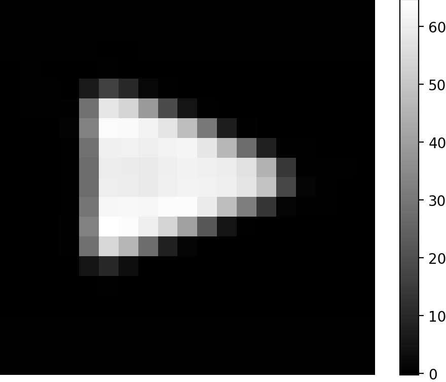
(a) Shape whitened, rSVD K=2000.

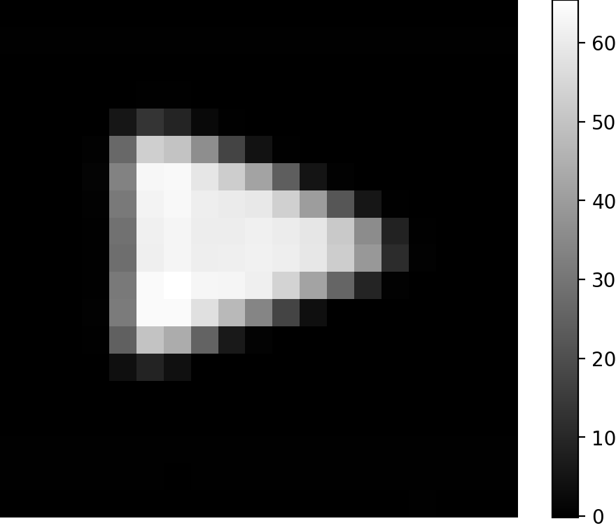
(b) Shape not whitened, rSVD K=2000.

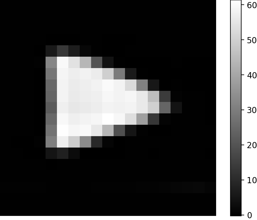
(c) Shape not whitened, rSVD K=6859.

Fig. 3: Reconstructions of the shape phantom using $\ell^{1}$-PnP with increasingly lower levels of preprocesssing.

In Fig. 3 a selected slice of the reconstructed shape phantom with different levels of preprocessing are displayed. We observe that the proposed $\ell^{1}$-PnP method is rather stable with respect to different preprocessing choices. Further, the results suggest the possibility of employing the $\ell^{1}$-PnP with less preprocessed data and our parameter selection strategy. In the next experiment we go a step further, not relying on preprocessing nor on the SVD.

3.5 Experiment 3: Reconstruction Without Preprocessing Based on Our Parameter Selection Strategy

In our third experiment we study the proposed $\ell^{1}$-PnP algorithm on not preprocessed data of the OpenMPI data set. In contrast to Experiment 2, we do not rely on any kind of SVD, neither for preprocessing, parameter selection, nor in the algorithmic part (Tikhonov type problem (9)). Employing methods not based on an SVD are important for future application scenarios since the computation of an SVD will become increasingly cumbersome with increasing problem size.

The dimension of the system matrix in this scenario is $151230\times 6859$. In particular, without the SVD we cannot solve the Euler-Lagrange equation (9) directly, so we use the Conjugated Gradient algorithm with a tolerance of $10^{-12}$ and a number of maximum iterations of $10000.$

Preprocessing

We do not perform any SNR thresholding, we do not whiten the data nor perform a rSVD. (However, we exclude the frequencies below 80 kHz.)

Parameters

We choose the parameters according to Sec 2.4. For roughly estimating the smallest singular values $\sigma_{\mathrm{min}}$ (without having a SVD) we use power iteration (cf. Section S5 in the supplementary material) and take into account the order of magnitude, i.e., we approximate $\sigma_{\mathrm{min}}$ by $10^{\lfloor\log_{10}\tau\rfloor}$ where $\tau$ denotes the calculated value; concretely, this results in a value of the estimate for $\sigma_{\mathrm{min}}$ as $10^{4}$.

(a) Shape 10-th xz-slice.

(b) Resolution 10-th xy-slice.

(c) Concentration 13-th xy-slice.

Fig. 4: Selected slices of the reconstructions obtained using the proposed $\ell^{1}$-PnP method with our parameter selection/stopping criterion strategy and no preprocessing of the data.

	Shape Ph.	Resolution Ph.	Concentration Ph.
PSNR	30.63	31.99	37.32
SSIM	0.951	0.749	0.570
stop it.	10	9	12

Table 5: Evaluation of the reconstructions using our parameter selection/stopping strategy and no preprocessing.

Results

Selected slices for each phantom in the Open MPI Dataset are shown in Fig. 4 and the quality evaluation with PSNR and SSIM is reported in Tab. 5. We observe that the result obtained in this experiments without preprocessing are comparable with the results obtained with the preprocessing and the knowledge of the SVD in Experiment 1 (cf. Tab. 2). The reconstruction time takes about 1 minute, 30 seconds of which are taken to move the full matrix $A$ to the GPU and to form the matrix $A^{*}A$. Finally, the reconstruction with the full matrix with the PnP approach here presented lasts about 30 seconds including the computation of the quantity $A^{*}f$.

4 Discussion and Conclusion

4.1 Discussion

We start out to discuss relations to the paper [4] which is to our knowledge the work closest to ours in the literature. The authors of [4] were the first to use a PnP method for MPI reconstruction. They train their denoiser on “MPI friendly” MRI data using data of images of vessels, more precisely, they derived their training data from time-of-flight cerebral magnetic resonance angiograms (MRA) to closely mimic the vascular structures targeted in their MPI scans. In contrast to [4], we use a different approach for denoising. We employ a larger size DNN which has been trained on a larger size data set consisting of natural images. The employed denoiser is not learned or transfer learned on MPI or similar MRI data. Our results underpin that larger architectures with larger sets of training data can generalize well to situations where the data distribution is not exactly as in the training data, in particular for conservative tasks such as denoising. This is particular appealing due to the very limited amount of (publicly) available MPI data. The authors of [4] provide a qualitative and quantitative evaluation on simulated data, and show the benefit of their PnP approach by qualitative evaluation on the resolution phantom of the Open MPI dataset. In contrast we here provided a quantitative and qualitative evaluation of our $\ell^{1}$-PnP approach on the full 3D Open MPI data set. Moreover, we use a different iterative scheme, namely the HQS, as a basis contrasting the ADMM type approach in [4]. Using HQS is appealing due to its simplicity. Finally, we provide strategies for parameter selection within our algorithm.

Secondly, we discuss the relation with the DIP approach. The DIP approach stands out since, to our knowledge, it is the only machine learning approach for which a qualitative and quantitative evalution has been carried out on the Open MPI dataset [14]. The DIP approach is an unsupervised approach acting on a single image only. This is on the one hand appealing since other training data cannot influence the reconstruction and on the other hand no training data is needed which is particularly appealing in the context of MPI. Although not an unsupervised approach, the proposed method shares the property that we need no training data (due to using the denoiser in a zero shot fashion.) However, the training data of the denoiser may influence the reconstruction where halucinating is less prominent in denoising. Moreover, the DIP approach suffers from high computational times whereas the $\ell^{1}$-PnP can converge in a few seconds for preprocessed data and in about 30 seconds for not preprocessed data.

4.2 Conclusion

In this work, we have developed a PnP approach with $\ell^{1}$-prior for MPI reconstruction using a generic zero-shot denoiser. In particular, we employed a larger size DNN, namely the DRUnet architecture of [70] which has been trained on a larger size data set consisting of natural images. In order to apply the image denoiser on a 3D volume, we employ slicing along the axes and averaging. We have quantitatively and qualitatively evaluated our approach on the full 3D Open MPI data set [39], which presently represents the only publicly available real MPI data set. To that end, we have employed suitable preprocessing, and we have compared our scheme quantitatively and qualitatively with the DIP approach of [14] as well as the Tikhonov regularization. Moreover, we have shown that the $\ell^{1}$-PnP approach proposed works with our parameter selection strategy and is able to perform fast reconstructions with different levels of preprocessing. In particular, we show that comparable results can be obtained without preprocessing and in particular without relying on a SVD.

Supplementary Material

S1 Description of the Background Scans

A delta probe is positioned at each grid cell that we can label with a triple $(x,y,z)$ for $x,y,z\in\{1,\cdots,19\}$. The scanning procedure proceeds in inverse lexicographic order of the tuples $(x,y,z)$, i.e., for any given $y$ and $z$, the scans are performed along the $x$-axis with $x$ from 1 to 19, then the $y$ variable is increased by 1. When all scans along $x$ are performed for each value $y$, the $z$ label is updated by 1. The background data - a scan without the delta probe - is collected at the beginning of the calibration process and each time the $y$ variable of the cell position is updated. Equivalently, the delta probe is removed and an empty scan is performed each time we complete the $19$ measurements along the $x$-axis for each $y$ and $z$. This many background scans are collected because the background signal is assumed to be dynamic. With this procedure, each scan of the delta probe $\delta_{(x,y,z)}$ is performed after an empty scan $b_{(y,z)}^{-}$ and before and empty scan $b_{(y,z)}^{+}$. We can correct each scan along the $x$-axis with the background correction obtained from the convex combination of $b_{(y,z)}^{-}$ and $b_{(y,z)}^{+}$, i.e., if $s_{(x,y,z)}$ is the signal collected scanning the delta probe in the cell $(x,y,z)$, and $\omega_{x}=\frac{x}{19}$ for $x=1,\dots,19$, then the background corrected signal $s_{(x,y,z)}^{\mathrm{corr.}}$ is:

$$s_{(x,y,z)}^{\mathrm{corr.}}=s_{(x,y,z)}-\left[\omega_{x}b_{(y,z)}^{-}+(1-\omega_{x})b_{(y,z)}^{+}\right].$$ (18)

S2 Specific Implementation of the SSIM

Given two images $f,g$, the SSIM is defined as

$$\mathrm{SSIM}(f,g)=\left[l(f,g)\right]^{\alpha}\cdot\left[c(f,g)\right]^{\beta}\cdot\left[s(f,g)\right]^{\gamma},$$

where

$$\begin{split}l(f,g)=\frac{2\mu_{f}\mu_{g}+C_{1}}{\mu_{x}^{2}+\mu_{y}^{2}+C_{1}},\\ c(f,g)=\frac{2\sigma_{f}\sigma_{g}+C_{2}}{\sigma_{x}^{2}+\sigma_{y}^{2}+C_{2}},\\ s(f,g)=\frac{\sigma_{fg}+C_{3}}{\sigma_{f}\sigma_{g}+C_{3}},\end{split}$$ (19)

are the luminance (l), contrast (c) and structure (s)  [64] and $\mu_{f}$ is the mean value, $\sigma_{f}$ the standard deviation of $f$; $\mu_{g}$ and $\sigma_{g}$ are analogously defined for $g$ and $\sigma_{fg}$ the covariance of $f$ and $g$. Following the implementation of [14], we set $\alpha=\beta=\gamma=1$ and $C_{1}=(0.01\cdot R)^{2}$, $C_{2}=(0.03\cdot R)^{2}$ and $C_{3}=0.5\cdot C_{2}$ where $R=100$, i.e., the concentration of the Delta Sample used during the calibration process.

S3 Description of the DIP

The minimization of the functional in Eq. (17) is performed with $p=1$ as suggested, with the random input $z$ having entries uniformly distributed in $[0,0.7]$ and the same shape of the output $(1,19,19,19)$; the regularizing architecture of $\varphi_{\theta}$ is an autoencoder obtained by not using skip connections in a U-Net with encoder steps that down-sample by a factor of 2 with 64, 128 and 256 channels respectively (the decoder is symmetric). The training of $\varphi_{\theta}$ has been performed minimizing the functional in Eq. (17) for 20000 iterations with Adam [30] with different learning rates $\alpha_{i}=10^{-i}$, for $i=3,4,5$ and momenta setting $\beta=(0.9,0.999)$. The selection strategy of the DIP reconstruction is the one used in [14]: we extract reconstructions after a number of iterations $s\in\{1,2,\dots,10,12,\dots,30,35,\dots,50,60,\dots,150,175,\dots,500,\\ 600,\dots,2000,2500,\dots,5000,6000,\dots 20000\}$. For each iteration $s$ we have computed the $\mathrm{PSNR}_{\mathrm{max}}$ and selected the iteration $s_{\mathrm{opt.}}$ that maximizes its value.

S4 Bounds on the $\ell^{1}$ Parameter $\alpha$

In each iteration, a soft-thresholding (proximal mapping of the $\ell^{1}$ norm) of parameter $\alpha/\mu_{k}$ is performed (cf. Eq. (11)). Let $u$ be the ground truth particle distribution and $u_{\mathrm{rec}}$ its reconstruction using the system matrix $A$. The matrix $A$ is obtained by scanning a delta distribution with a known concentration of $c_{\delta}$ mmol. It follows that if $c_{u}$ is the maximum concentration level of the ground truth $u$, the $\ell^{\infty}$-norm of the reconstruction is bounded from above $\lVert u_{\mathrm{rec}}\rVert_{\infty}\leq c_{u}/c_{\delta}=:c_{\mathrm{rec}}$. Therefore, to avoid that the soft-thresholding totally compresses the reconstruction, it is necessary that $\alpha/\mu_{k}<c_{\mathrm{rec}}$, i.e., that $\alpha<c_{\mathrm{rec}}\cdot\mu_{0}$. In particular, if some knowledge about the concentration injected and the concentration of the delta distribution is available, it is possible to set a rough bound on the parameter $\alpha$, for example $\alpha<5\%\cdot c_{\mathrm{rec}}\cdot\mu_{0}$ if we want to allow compression of at most $5\%$ of the reconstructed concentration level. In the experiments in Section 3, because in the Open MPI Dataset $c_{\delta}=100$mmol and we know that for each phantom $c_{u}\leq 100$mmol, we can deduce that $c_{\mathrm{rec}}\leq 1$ and that $\alpha\leq\mu_{0}$. In particular, we choose to compress below $0.5\%$ of the concentration level and set for all experiments in Section 3 the parameter $\alpha=\frac{5}{1000}\mu_{0}$.

S5 Power Iteration Method for $\sigma_{\mathrm{min}}$

We consider the matrix $A^{*}A$ and use the power iteration to approximate $\sigma_{\mathrm{max}}^{2}$, then we apply the power iteration method once more to the matrix $A^{*}A-\sigma_{\mathrm{max}}^{2}\mathrm{Id_{N}}$ to approximate its eigenvalue with greatest norm, i.e., $\tilde{\sigma}_{\mathrm{max}}^{2}=\sigma_{\mathrm{min}}^{2}-\sigma_{\mathrm{max}}^{2}$ and can retrieve an approximation of the smallest singular value $\sigma_{\mathrm{min}}^{2}=\tilde{\sigma}_{\mathrm{max}}^{2}+\sigma_{\mathrm{max}}^{2}$.

S6 Results of Experiment 1

in x,y,z

ıin 1,…,5

(a) CAD, ı-th slice along .

(b) Tikhonov, ı-th slice along .

(c) DIP, ı-th slice along .

(d) PnP, ı-th slice along .

Fig. S1: Shape phantom in Experiment 1, slices along the -axis from 1 to 5

ıin 6,…,10

(a) CAD, ı-th slice along .

(b) Tikhonov, ı-th slice along .

(c) DIP, ı-th slice along .

(d) PnP, ı-th slice along .

Fig. S2: Shape phantom in Experiment 1, slices along the -axis from 6 to 10

ıin 11,…,15

(a) CAD, ı-th slice along .

(b) Tikhonov, ı-th slice along .

(c) DIP, ı-th slice along .

(d) PnP, ı-th slice along .

Fig. S3: Shape phantom in Experiment 1, slices along the -axis from 11 to 15

ıin 16,…,19

(a) CAD, ı-th slice along .

(b) Tikhonov, ı-th slice along .

(c) DIP, ı-th slice along .

(d) PnP, ı-th slice along .

Fig. S4: Shape phantom in Experiment 1, slices along the -axis from 16 to 19

in x,y,z

ıin 1,…,5

(a) CAD, ı-th slice along .

(b) Tikhonov, ı-th slice along .

(c) DIP, ı-th slice along .

(d) PnP, ı-th slice along .

Fig. S5: Resolution phantom in Experiment 1, slices along the -axis from 1 to 5

ıin 6,…,10

(a) CAD, ı-th slice along .

(b) Tikhonov, ı-th slice along .

(c) DIP, ı-th slice along .

(d) PnP, ı-th slice along .

Fig. S6: Resolution phantom in Experiment 1, slices along the -axis from 6 to 10

ıin 11,…,15

(a) CAD, ı-th slice along .

(b) Tikhonov, ı-th slice along .

(c) DIP, ı-th slice along .

(d) PnP, ı-th slice along .

Fig. S7: Resolution phantom in Experiment 1, slices along the -axis from 11 to 15

ıin 16,…,19

(a) CAD, ı-th slice along .

(b) Tikhonov, ı-th slice along .

(c) DIP, ı-th slice along .

(d) PnP, ı-th slice along .

Fig. S8: Resolution phantom in Experiment 1, slices along the -axis from 16 to 19

in x,y,z

ıin 1,…,5

(a) CAD, ı-th slice along .

(b) Tikhonov, ı-th slice along .

(c) DIP, ı-th slice along .

(d) PnP, ı-th slice along .

Fig. S9: Concentration phantom in Experiment 1, slices along the -axis from 1 to 5

ıin 6,…,10

(a) CAD, ı-th slice along .

(b) Tikhonov, ı-th slice along .

(c) DIP, ı-th slice along .

(d) PnP, ı-th slice along .

Fig. S10: Concentration phantom in Experiment 1, slices along the -axis from 6 to 10

ıin 11,…,15

(a) CAD, ı-th slice along .

(b) Tikhonov, ı-th slice along .

(c) DIP, ı-th slice along .

(d) PnP, ı-th slice along .

Fig. S11: Concentration phantom in Experiment 1, slices along the -axis from 11 to 15

ıin 16,…,19

(a) CAD, ı-th slice along .

(b) Tikhonov, ı-th slice along .

(c) DIP, ı-th slice along .

(d) PnP, ı-th slice along .

Fig. S12: Concentration phantom in Experiment 1, slices along the -axis from 16 to 19

S7 Results of Experiment 3.

in x,y,z

ıin 1,…,10

(a) CAD, ı-th slice along .

(b) PnP, ı-th slice along .

Fig. S13: Shape phantom in Experiment 3, slices along the -axis from 1 to 10

ıin 11,…,19

(a) CAD, ı-th slice along .

(b) PnP, ı-th slice along .

Fig. S14: Shape phantom in Experiment 3, slices along the -axis from 11 to 19.

in x,y,z

ıin 1,…,10

(a) CAD, ı-th slice along .

(b) PnP, ı-th slice along .

Fig. S15: Resolution phantom in Experiment 3, slices along the -axis from 1 to 10

ıin 11,…,19

(a) CAD, ı-th slice along .

(b) PnP, ı-th slice along .

Fig. S16: Resolution phantom in Experiment 3, slices along the -axis from 11 to 19.

in x,y,z

ıin 1,…,10

(a) CAD, ı-th slice along .

(b) PnP, ı-th slice along .

Fig. S17: Concentration phantom in Experiment 3, slices along the -axis from 1 to 10

ıin 11,…,19

(a) CAD, ı-th slice along .

(b) PnP, ı-th slice along .

Fig. S18: Concentration phantom in Experiment 3, slices along the -axis from 11 to 19.

References

- [1] E. Agustsson and R. Timofte, NTIRE 2017 Challenge on Single Image Super-Resolution: Dataset and Study, in 2017 IEEE Conference on Computer Vision and Pattern Recognition Workshops (CVPRW), 2017, pp. 1122–1131.
- [2] R. Ahmad, C. A. Bouman, G. T. Buzzard, S. Chan, S. Liu, E. T. Reehorst, and P. Schniter, Plug-and-Play Methods for Magnetic Resonance Imaging: Using Denoisers for Image Recovery, IEEE Signal Processing Magazine, 37 (2020), pp. 105–116.
- [3] H. Arami, E. Teeman, A. Troksa, H. Bradshaw, K. Saatchi, A. Tomitaka, S. S. Gambhir, U. O. Häfeli, D. Liggitt, and K. M. Krishnan, Tomographic Magnetic Particle Imaging of Cancer Targeted Nanoparticles, Nanoscale, 9 (2017), pp. 18723–18730.
- [4] B. Askin, A. Güngör, D. Alptekin Soydan, E. U. Saritas, C. B. Top, and T. Cukur, Pp-mpi: A deep plug-and-play prior for magnetic particle imaging reconstruction, in International Workshop on Machine Learning for Medical Image Reconstruction (In conjunction with MICCAI), Springer, 2022, pp. 105–114.
- [5] S. Bai, J. Z. Kolter, and V. Koltun, Deep equilibrium models, in Advances in Neural Information Processing Systems, H. Wallach, H. Larochelle, A. Beygelzimer, F. d’ Alché-Buc, E. Fox, and R. Garnett, eds., Curran Associates, Inc.
- [6] A. Bakenecker, M. Ahlborg, C. Debbeler, C. Kaethner, T. Buzug, and K. Lüdtke-Buzug, Magnetic Particle Imaging in Vascular Medicine, Innovative Surgical Sciences, 3 (2018), pp. 179–192.
- [7] M. Bertero, P. Boccacci, and C. De Mol, Introduction to Inverse Problems in Imaging, CRC press, 2021.
- [8] C. Billings, M. Langley, G. Warrington, F. Mashali, and J. A. Johnson, Magnetic Particle Imaging: Current and Future Applications, Magnetic Nanoparticle Synthesis Methods and Safety Measures, International Journal of Molecular Sciences, 22 (2021).
- [9] G. Bringout, W. Erb, and J. Frikel, A new 3D Model for Magnetic Particle Imaging Using Realistic Magnetic Field Topologies for Algebraic Reconstruction, Inverse Problems, 36 (2020), p. 124002.
- [10] T. M. Buzug, Computed Tomography From Photon Statistics to Modern Cone-Beam CT, Springer, Germany, 2008.
- [11] Y. Chen and T. Pock, Trainable Nonlinear Reaction Diffusion: A Flexible Framework for Fast and Effective Image Restoration, IEEE Transactions on Pattern Analysis and Machine Intelligence, 39 (2017), pp. 1256–1272.
- [12] J. Connell, P. Patrick, Y. Yu, M. Lythgoe, and T. Kalber, Advanced Cell Therapies: Targeting, Tracking and Actuation of Cells with Magnetic Particles, Regenerative medicine, 10 (2015), pp. 757–72.
- [13] I. Daubechies, M. Defrise, and C. D. Mol, An Iterative Thresholding Algorithm for Linear Inverse Problems with a Aparsity Constraint, Communications on Pure and Applied Mathematics, 57 (2003).
- [14] S. Dittmer, T. Kluth, M. T. R. Henriksen, and P. Maass, Deep Image Prior for 3D Magnetic Particle Imaging: A Quantitative Comparison of Regularization Techniques on Open MPI Dataset, Int. J. Mag. Part. Imag., 7 (2021).
- [15] Y. Du, X. Liu, Q. Liang, X.-J. Liang, and J. Tian, Optimization and Design of Magnetic Ferrite Nanoparticles with Uniform Tumor Distribution for Highly Sensitive MRI/MPI Performance and Improved Magnetic Hyperthermia Therapy, Nano Letters, 19 (2019), pp. 3618–3626.
- [16] J. Franke, N. Baxan, H. Lehr, U. Heinen, S. Reinartz, J. Schnorr, M. Heidenreich, F. Kiessling, and V. Schulz, Hybrid MPI-MRI System for Dual-Modal In Situ Cardiovascular Assessments of Real-Time 3D Blood Flow Quantification - A Pre-Clinical In Vivo Feasibility Investigation, IEEE Transactions on Medical Imaging, 39 (2020), pp. 4335–4345.
- [17] B. Gleich and J. Weizenecker, Tomographic Imaging Using the Nonlinear Response of Magnetic Particles, Nature, 435 (2005), pp. 1214–1217.
- [18] P. Goodwill and S. M. Conolly, The X-Space Formulation of the Magnetic Particle Imaging Process: 1-D Signal, Resolution, Bandwidth, SNR, SAR, and Magnetostimulation, IEEE Trans. Med. Imaging, 29 (2010), pp. 1851–1859.
- [19] , Multidimensional X-Space Magnetic Particle Imaging, IEEE Trans. Med. Imaging, 30 (2011), pp. 1581–1590.
- [20] M. Graeser, F. Thieben, P. Szwargulski, F. Werner, N. Gdaniec, M. Boberg, F. Griese, M. Möddel, P. Ludewig, D. van de Ven, O. M. Weber, O. Woywode, B. Gleich, and T. Knopp, Human-Sized Magnetic Particle Imaging for Brain Applications, Nature Communications, 10 (2019), p. 1936.
- [21] M. Grüttner, T. Knopp, J. Franke, M. Heidenreich, J. Rahmer, A. Halkola, C. Kaethner, J. Borgert, and T. M. Buzug, On the Formulation of the Image Reconstruction Problem in Magnetic Particle Imaging, Biomedical Engineering, 58 (2013), pp. 583–591.
- [22] A. Güngör, B. Askin, D. A. Soydan, C. Barış Top, and T. Cukur, Deep Learned Super Resolution of System Matrices for Magnetic Particle Imaging, in 43rd Annual International Conference of the IEEE Engineering in Medicine & Biology Society, 2021, pp. 3749–3752.
- [23] A. Güngör, B. Askin, D. A. Soydan, E. U. Saritas, C. B. Top, and T. Çukur, TranSMS: Transformers for Super-Resolution Calibration in Magnetic Particle Imaging, IEEE Transactions on Medical Imaging, 41 (2022), pp. 3562–3574.
- [24] A. Güngör, B. Askin, D. A. Soydan, C. B. Top, E. U. Saritas, and T. Çukur, DEQ-MPI: A Deep Equilibrium Reconstruction with Learned Consistency for Magnetic Particle Imaging, IEEE Transactions on Medical Imaging, (2023), pp. 1–1.
- [25] J. Haegele, J. Rahmer, B. Gleich, J. Borgert, H. Wojtczyk, N. Panagiotopoulos, T. M. Buzug, J. Barkhausen, and F. M. Vogt, Magnetic Particle Imaging: Visualization of Instruments for Cardiovascular Intervention, Radiology, 265 (2012), pp. 933–938.
- [26] N. Halko, P. Martinsson, and J. Tropp, Finding Structure with Randomness: Probabilistic Algorithms for Constructing Approximate Matrix Decompositions, SIAM Review, 53 (2011), pp. 217–288.
- [27] T. Hatsuda, S. Shimizu, H. Tsuchiya, T. Takagi, T. Noguchi, and Y. Ishihara, A basic study of an image reconstruction method using neural networks for magnetic particle imaging, in 5th International Workshop on Magnetic Particle Imaging, IEEE, 2015, pp. 1–1.
- [28] K. He, X. Zhang, S. Ren, and J. Sun, Deep Residual Learning for Image Recognition, in 2016 IEEE Conference on Computer Vision and Pattern Recognition (CVPR), 2016, pp. 770–778.
- [29] K. O. Jung, H. Jo, J. H. Yu, S. S. Gambhir, and G. Pratx, Development and MPI Tracking of Novel Hypoxia-Targeted Theranostic Exosomes, Biomaterials, 177 (2018), pp. 139–148.
- [30] D. P. Kingma and J. Ba, Adam: A Method for Stochastic Optimization, in 3rd International Conference on Learning Representations 2015, Y. Bengio and Y. LeCun, eds., 2015.
- [31] T. Kluth and B. Jin, Enhanced Reconstruction in Magnetic Particle Imaging by Whitening and Randomized SVD Approximation, Phys Med Biol, 64 (2019), p. 125026.
- [32] , L1 Data Fitting for Robust Reconstruction in Magnetic Particle Imaging: Quantitative Evaluation on Open MPI Dataset, Int J Mag Part Imag, 6 (2020).
- [33] T. Kluth, B. Jin, and G. Li, On the degree of ill-posedness of multi-dimensional magnetic particle imaging, Inverse Problems, 34 (2018), p. 095006.
- [34] T. Knopp, S. Biederer, T. Sattel, and T. M. Buzug, Singular value analysis for magnetic particle imaging, in 2008 IEEE Nuclear Science Symposium Conference Record, IEEE, 2008, pp. 4525–4529.
- [35] T. Knopp, S. Biederer, T. Sattel, M. Erbe, and T. Buzug, Prediction of the Spatial Resolution of Magnetic Particle Imaging Using the Modulation Transfer Function of the Imaging Process, IEEE Transactions on Medical Imaging, 30 (2011), pp. 1284–1292.
- [36] T. Knopp, S. Biederer, T. F. Sattel, J. Rahmer, J. Weizenecker, B. Gleich, J. Borgert, and T. M. Buzug, 2D Model-Based Reconstruction for Magnetic Particle Imaging, Medical Physics, 37 (2010), pp. 485–491.
- [37] T. Knopp and T. M. Buzug, Magnetic Particle Imaging: An Introduction to Imaging Principles and Scanner Instrumentation, Springer, 2012.
- [38] T. Knopp, J. Rahmer, T. Sattel, S. Biederer, J. Weizenecker, B. Gleich, J. Borgert, and T. Buzug, Weighted Iterative Reconstruction for Magnetic Particle Imaging, Physics in Medicine and Biology, 55 (2010), pp. 1577–1589.
- [39] T. Knopp, P. Szwargulski, F. Griese, and M. Gräser, OpenMPIData: An Initiative for Freely Accessible Magnetic Particle Imaging Data, Data in brief, 28 (2020), p. 104971.
- [40] D. Kuhl and R. Edwards, Image Separation Radioisotope Scanning, Radiology, 80 (1963), pp. 653–662.
- [41] J. Lampe, C. Bassoy, J. Rahmer, J. Weizenecker, H. Voss, B. Gleich, and J. Borgert, Fast Reconstruction in Magnetic Particle Imaging, Phys. Med. Biol., 57 (2012), pp. 1113–1134.
- [42] J. E. Lemaster, F. Chen, T. Kim, A. Hariri, and J. V. Jokerst, Development of a Trimodal Contrast Agent for Acoustic and Magnetic Particle Imaging of Stem Cells, ACS Applied Nano Materials, 1 (2018), pp. 1321–1331.
- [43] B. Lim, S. Son, H. Kim, S. Nah, and K. M. Lee, Enhanced Deep Residual Networks for Single Image Super-Resolution, in 2017 IEEE Conference on Computer Vision and Pattern Recognition Workshops (CVPRW), 2017, pp. 1132–1140.
- [44] K. Ma, Z. Duanmu, Q. Wu, Z. Wang, H. Yong, H. Li, and L. Zhang, Waterloo Exploration Database: New Challenges for Image Quality Assessment Models, IEEE Transactions on Image Processing, 26 (2017), pp. 1004–1016.
- [45] T. März and A. Weinmann, Model-Based Reconstruction for Magnetic Particle Imaging in 2D and 3D, Inverse Problems & Imaging, 10 (2016), pp. 1087–1110.
- [46] Orendorff, Ryan and Peck, Austin J and Zheng, Bo and Shirazi, Shawn N and Matthew Ferguson, R and Khandhar, Amit P and Kemp, Scott J and Goodwill, Patrick and Krishnan, Kannan M and Brooks, George A and Kaufer, Daniela and Conolly, Steven, First in Vivo Traumatic Brain Injury Imaging via Magnetic Particle Imaging, Phys Med Biol, 62 (2017), pp. 3501–3509.
- [47] J. Rahmer, J. Weizenecker, B. Gleich, and J. Borgert, Signal Encoding in Magnetic Particle Imaging: Properties of the System Function, BMC Medical Imaging, 9 (2009), p. 4.
- [48] J. Rahmer, J. Weizenecker, B. Gleich, and J. Borgert, Analysis of a 3-D System Function Measured for Magnetic Particle Imaging, IEEE Trans. Med. Imaging, 31 (2012), pp. 1289–1299.
- [49] O. Ronneberger, P. Fischer, e. N. Brox, Thomas", J. Hornegger, W. M. Wells, and A. F. Frangi, U-Net: Convolutional Networks for Biomedical Image Segmentation, in Medical Image Computing and Computer-Assisted Intervention – MICCAI 2015, Springer International Publishing, 2015, pp. 234–241.
- [50] I. Schmale, B. Gleich, J. Rahmer, C. Bontus, J. Schmidt, and J. Borgert, MPI Safety in the View of MRI Safety Standards, IEEE Transactions on Magnetics, 51 (2015), pp. 1–4.
- [51] H. Schomberg, Magnetic Particle Imaging: Model and Reconstruction, in 2010 IEEE International Symposium on Biomedical Imaging: From Nano to Macro, 2010, pp. 992–995.
- [52] F. Schrank, D. Pantke, and V. Schulz, Deep learning MPI Super-Resolution by Implicit Representation of the System Matrix, vol. 8, 2022.
- [53] Y. Shang, J. Liu, L. Zhang, X. Wu, P. Zhang, L. Yin, H. Hui, and J. Tian, Deep Learning for Improving the Spatial Resolution of Magnetic Particle Imaging, Physics in Medicine & Biology, 67 (2022), p. 125012.
- [54] G. Song, M. Chen, Y. Zhang, L. Cui, H. Qu, X. Zheng, M. Wintermark, Z. Liu, and J. Rao, Janus Iron Oxides @ Semiconducting Polymer Nanoparticle Tracer for Cell Tracking by Magnetic Particle Imaging, Nano Letters, 18 (2018), pp. 182–189.
- [55] S. Sreehari, S. V. Venkatakrishnan, B. Wohlberg, G. T. Buzzard, L. F. Drummy, J. P. Simmons, and C. A. Bouman, Plug-and-play priors for bright field electron tomography and sparse interpolation, IEEE Transactions on Computational Imaging, 2 (2016), pp. 408–423.
- [56] M. Storath, C. Brandt, M. Hofmann, T. Knopp, J. Salamon, A. Weber, and A. Weinmann, Edge Preserving and Noise Reducing Reconstruction for Magnetic Particle Imaging, IEEE Transactions on Medical Imaging, 36 (2017), pp. 74–85.
- [57] Y. Sun, B. Wohlberg, and U. S. Kamilov, An online plug-and-play algorithm for regularized image reconstruction, IEEE Transactions on Computational Imaging, 5 (2019), pp. 395–408.
- [58] Z. W. Tay, P. Chandrasekharan, B. D. Fellows, I. R. Arrizabalaga, E. Yu, M. Olivo, and S. M. Conolly, Magnetic Particle Imaging: An Emerging Modality with Prospects in Diagnosis, Targeting and Therapy of Cancer, Cancers (Basel), 13 (2021).
- [59] M. Ter-Pogossian, M. Phelps, E. Hoffman, and N. Mullani, A Positron-Emission Transaxial Tomograph for Nuclear Imaging (PETT), Radiology, 114 (1975), pp. 89–98.
- [60] W. Tong, H. Hui, W. Shang, Y. Zhang, F. Tian, Q. Ma, X. Yang, J. Tian, and Y. Chen, Highly Sensitive Magnetic Particle Imaging of Vulnerable Atherosclerotic Plaque with Active Myeloperoxidase-Targeted Nanoparticles, Theranostics, 11 (2021), pp. 506–521.
- [61] D. Ulyanov, A. Vedaldi, and V. Lempitsky, Deep Image Prior, in Proceedings of the IEEE CVPR, 2018, pp. 9446–9454.
- [62] S. Vaalma, J. Rahmer, N. Panagiotopoulos, R. L. Duschka, J. Borgert, J. Barkhausen, F. M. Vogt, and J. Haegele, Magnetic Particle Imaging (MPI): Experimental Quantification of Vascular Stenosis Using Stationary Stenosis Phantoms, PLOS ONE, 12 (2017), pp. 1–22.
- [63] A. von Gladiss, R. Memmesheimer, N. Theisen, A. Bakenecker, T. Buzug, and D. Paulus, Reconstruction of 1d images with a neural network for magnetic particle imaging, in ProceedingsmGerman Workshop on Medical Image Computing, Heidelberg, June 26-28, 2022, Springer, 2022, pp. 247–252.
- [64] Z. Wang, E. Simoncelli, and A. Bovik, Multiscale structural similarity for image quality assessment, in The Thrity-Seventh Asilomar Conference on Signals, Systems & Computers, 2003, vol. 2, 2003, pp. 1398–1402 Vol.2.
- [65] J. Weizenecker, J. Borgert, and B. Gleich, A Simulation Study on the Resolution and Sensitivity of Magnetic Particle Imaging, Phys. Med. Biol., 52 (2007), pp. 6363–6374.
- [66] J. Weizenecker, B. Gleich, J. Rahmer, H. Dahnke, and J. Borgert, Three-Dimensional Real-Time in Vivo Magnetic Particle Imaging, Phys. Med. Biol., 54 (2009), pp. L1–L10.
- [67] X. Yang, G. Shao, Y. Zhang, W. Wang, Y. Qi, S. Han, and H. Li, Applications of Magnetic Particle Imaging in Biomedicine: Advancements and Prospects, Front Physiol, 13 (2022), p. 898426.
- [68] L. Yin, H. Guo, P. Zhang, Y. Li, H. Hui, Y. Du, and J. Tian, System Matrix Recovery Based on Deep Image Prior in Magnetic Particle Imaging, Physics in Medicine & Biology, 68 (2023), p. 035006.
- [69] E. Yu, M. Bishop, B. Zheng, R. M. Ferguson, A. Khandhar, S. Kemp, K. Krishnan, P. Goodwill, and S. Conolly, Magnetic Particle Imaging: A Novel in Vivo Imaging Platform for Cancer Detection, Nano Letters, 17 (2017), pp. 1648–1654.
- [70] K. Zhang, Y. Li, W. Zuo, L. Zhang, L. Van Gool, and R. Timofte, Plug-and-Play Image Restoration With Deep Denoiser Prior, IEEE Transactions on Pattern Analysis and Machine Intelligence, 44 (2022), pp. 6360–6376.
- [71] X. Y. Zhou, K. E. Jeffris, E. Y. Yu, B. Zheng, P. W. Goodwill, P. Nahid, and S. M. Conolly, First in Vivo Magnetic Particle Imaging of Lung Perfusion in Rats, Physics in Medicine & Biology, 62 (2017), p. 3510.
- [72] X. Zhu, J. Li, P. Peng, N. Hosseini Nassab, and B. R. Smith, Quantitative Drug Release Monitoring in Tumors of Living Subjects by Magnetic Particle Imaging Nanocomposite, Nano Letters, 19 (2019), pp. 6725–6733.