Forensic Science and
How Statistics Can Help It
Evidence, Hypothesis Testing, and Graphical Models

Abstract

In the United States, the persistent issue of innocent individuals being wrongly convicted emphasizes the need for scrutiny and improvement in the criminal justice system. It is particularly crucial to establish national-level standards addressing statistical aspects, including the analysis, interpretation, and reporting of forensic evidence. In this paper, we discuss the main types of evidence used in forensic investigations, including glass, fingerprints, and DNA. We also examine the challenges in promoting statistics in court and how they can be overcome. Finally, we delve into the likelihood ratio framework and graphical models and their applications in forensic evidence evaluation, particularly in DNA typing.

Keywords: forensic statistics, evidence evaluation, hypothesis testing, likelihood ratio, graphical models.

1 Introduction

Innocent individuals being wrongly convicted of serious crimes is a recurring occurrence in the United States. Recently, there has been significant focus on cases of wrongful convictions [1]. According to the National Registry of Exonerations 2022 Annual Report, 233 exonerations have occurred in the United States in 2022, among which, 44 cases involved false or misleading forensic evidence [2].

In the United States, trial courts handle a wide variety of case types, which can be broadly categorized into two groups: civil cases and criminal cases [3]. Civil cases typically revolve around conflicts related to finances, property, or constitutional rights. These disputes may be initiated by an individual, corporation, or government agency through a civil lawsuit. Criminal cases pertain to the accusation of breaching federal criminal statutes and only the government can initiate the criminal proceedings [4]. The court system and set of rules for handling both civil and criminal cases vary between states, but for criminal cases they are similar to the federal rules that can be found in the Federal Rules of Criminal Procedure [5].

The general steps of a federal criminal process in the U.S.A. are shown in Figure 1, which is not exhaustive and can be simpler or more complex for specific cases.

Figure 1: Federal criminal process. Forensic evidence plays a crucial role throughout the whole process.

The investigation step is where agencies such as Federal Bureau of Investigation (FBI), Drug Enforcement Administration (DEA), Bureau of Alcohol, Tobacco, Firearms and Explosives (ATF), United States Secret Service (USSS), Homeland Security Investigations (DHS/HSI), employ criminal investigators to gather and provide information to the United States Attorneys (the prosecutors) within their designated areas. Upon reviewing the information provided by investigators and conducting interviews with relevant individuals, the prosecutor assesses whether to submit the case to a grand jury, which is approximately made up of 16-23 members. For potential felony charges, the grand jury will be presented the evidence, witnesses’ testimony, along with a summary of the case provided by the prosecutor, based on which they would confidentially vote to determine if there is sufficient evidence to formally charge the individual with a crime. Typically within a day or two following a defendant’s arrest and formal charges, they are brought before a magistrate judge for an initial case hearing, where the judge decides whether the defendant will be detained in custody or released until the trial. The government and the defendant can both avoid the trial by offering a plea deal or pleading guilty, respectively. Afterwards, both the prosecutor and the defense attorney prepare for the trial, in order to become familiar about the details of the crime. They usually engage in discussions with witnesses (lay witnesses, expert witnesses and character witnesses), analyze the available evidence, predict potential trial complications, and formulate a strategic approach for the trial. After the optional preliminary hearing where the prosecutor shows that there is enough evidence (including evidence that cannot be shown to the jury) to charge the defendant, the lawsuit then enters the trial stage, which consists of pre-trial motions (motion to dismiss, motion to suppress, motion for change of venue), the trial, and post-trial motions (motion for a new trial, motion for judgment of acquittal, motion to vacate, set aside, or correct a sentence). The trial is a formal procedure in which the prosecutor seeks to convince the jury of the defendant’s guilt, whereas the defendant, aided by the attorney, presents their perspective, both through witnesses and evidence. The jury then assesses whether the defendant is innocent or guilty based on the presented evidence. The defendant return to the court to be sentenced usually a few months after the defendant is found guilty, based on the minimum and maximum punishments set by the Congress and the sentencing guidelines for recommended punishments considering different factors produced by the United States Sentencing Commissions. If the defendant believes there was an unjust verdict or if the sentence was overly severe, they have the opportunity to appeal to the Circuit Court following an conviction. They are also allowed to try to appeal the decision by the Circuit Court to the United States Supreme Court in Washington, D.C., which is the highest appellate court in the American court system and will make the final decision about the defendant’s appeal [6].

During the federal criminal process, examiners need to cope with uncertainties, especially when intepreting forensic evidence. Statistical thinking and computation are getting emphasized [7]. In 2009, the National Research Council published a report titled Strengthening Forensic Science in the United States: A Path Forward for the purpose of setting standards in forensic science, including statistical analysis [8].

In this paper we describe the important role played by statistics in forensic science. Section 2 introduces different types of evidence commonly used in court. Section 3 discusses the obstacles faced by the use of statistics in court. Section 4 and Section 5 introduce the two major frameworks of statistics used in court, i.e., likelihood ratio framework and graphical models. Finally, in Section 6 we provide some final remarks and discuss future research directions.

2 Evidence

Criminals in ancient world could easily avoid punishment due to limited standardized forensic practices. These practices typically were constrained to forced confession, witness statements, and arguments between prosecutors and defenders [9], which were subject to errors and coercion. The world’s first written documentation in forensic medicine is credited to Chinese author Song Ci’s Xi Yuan Ji Lu (translated as Collected Writings on the Washing Away of Wrongs) written in the 13th century [10]. Over the centuries, forensic science has evolved into a broad field that is now a common tool in criminal and civil law.

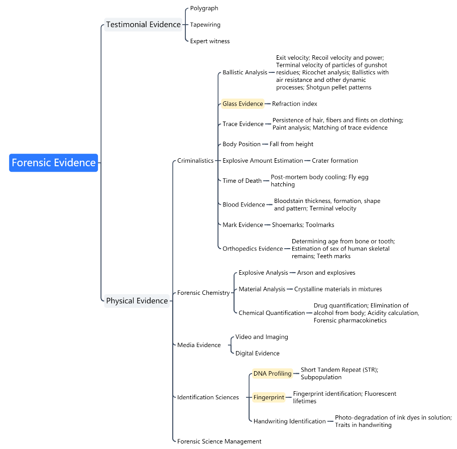
Evidence is generally categorized into testimonial and non-testimonial evidence. Testimonial evidence is one of the oldest types of evidence in human history. The word “testimony” and “testify” both originates from the Latin word testis, which refers to the concept related to a disinterested third-party witness [11]. Especially in ancient society, with the lack of standardized forensic practices, the results of trials relied heavily on witness statements [9]. Non-testimonial or physical evidence can be categorized into criminalistics, forensic chemistry, media evidence, identification science, and forensic science management, according to the 19th International Forensic Science Symposium (October 2019, France) sponsored by Interpol [12]. Based on this categorization and several other sources [13, 14, 15], we built a mind map (Figure 2) that organizes the various types of forensic evidence commonly used in court. In the rest of this section, we provide details about common types of physical evidence, in particular glass, fingerprint, and DNA, which will be discussed further in subsequent sections on statistical methods.

Figure 2: Mind map of forensic evidence. Forensic evidence is generally categorized into testimonial and non-testimonial or physical evidence. Physical evidence is categorized into criminalistics, forensic chemistry, media evidence, identification science, and forensic science management.

2.1 Glass

Usually, glass evidence comes from a broken window, but it may also arise from headlight or windshield glass in a car accident, bottles in an assault case, containers in a domestic violence case or laboratory accident [16]. Glass evidence is routinely used in the reconstruction of events, for example, to link an individual or an item to the crime scene or a victim [17]. This is accomplished by aligning the refractive index (RI) of the “recovered” sample (the set of fragments recovered from the suspect) and the “control” sample (fragments sampled from the crime scene) with the silicon oil of known RI in which the samples are submerged. The RI of glass fragments can be considered constant, while the RI of the oil changes linearly with temperature. By changing the temperature of the silicon oil with a glass sample submerged, the edge of the glass fragments will become invisible when the RI of the glass fragment and the oil are the same [18]. We can therefore obtain the RI of control and recovered samples and apply t-test to test if they are significantly different [13].

2.2 Fingerprint

In 1892, two children were found murdered in Buenos Aires, Argentina. Francisca Rojas, the mother of the children, accused a man named Velasquez of the murders due to jealousy over her relationship with another man. Despite being violently beaten by the local authority, Velasquez did not admit to the crime. Meanwhile, inspector Eduardo Alvarez found a bloody thumbprint on the door at the crime scene which matched the print of Francisca Rojas herself and she subsequently confessed to the murders [19, 20]. This case is notable as the first homicide investigation and trial in which fingerprint evidence played a critical role [21, 22].

Fingerprint friction ridge details are typically categorized into three hierarchical levels (see [23]). The first level involves the overall pattern of the ridges, which includes loops, whorls, and arches. While this level cannot be used for individualization, it can help to exclude suspects from consideration [24]. The second level of detail involves minutiae points, also known as Galton characteristics, which refer to specific path of the friction ridges. This level has sufficient discriminating power [25, 26] and was first quantitatively studied by Francis Galton in 1872 using a probabilistic analysis [24, 27]. The third level of detail involves the intrinsic ridge shapes and relative pore locations [24]. Although latent fingerprint resolution may not always be high enough to extract level-3 details, these features can be helpful for qualitative examination as they are also permanent, immutable, and unique. According to a study on pore identification conducted by Locard in 1912, 20 to 40 pores should be sufficient to identify a person [24].

2.3 DNA

DNA (deoxyribonucleic acid) analysis in forensic investigations has quickly emerged as an indispensable tool in the identification of suspects, the establishment of guilt in criminal cases, and promoting the precision and equity in the criminal justice system since its first introduction to forensic science in the mid 1980s [28, 29, 30]. As an illustration, in 1999, DNA evidence helped New York authorities to establish the connection between a man and at least 22 incidents of sexual assaults and robberies that had instilled fear in the city. In 2002, authorities in Philadelphia, Pennsylvania and Fort Collins, Colorado utilized DNA evidence to link and resolve a string of rapes and a murder committed by the same individual. In 2001, DNA evidence served as a significant breakthrough in the “Green River Killings” that had remained unsolved for years, despite extensive efforts by law enforcement and a $15 million investigation [29].

The first step of the DNA typing process is to separate the DNA molecules from other cellular materials that are contained in the sample, which is usually in the form of blood stain, semen stain, or liquid blood sample. To ensure optimal results, examiners also need to measure the quantity and quality of DNA before further processing. Then, the two strands are heated and separated, and enzymes known as primers will bind to the regions known as loci that are targeted for polymerase chain reaction (PCR) amplification [31].

The primary technology for quantitative analysis of DNA evidence is known as short tandem repeat (STR). This method focuses on the short sequences of base pairs that occur at specific loci along DNA strands [31, 13]. For example, there are repeated sequences of base pairs $[\text{GATA}]_{n}$ on chromosome 16 in human at locus D16S539, where $n$ typically ranges from 5 to 15. Each distinct sequence is referred to as an allele. An example of an allele is

GATAGATAGATAGATAGATAGATAGATAGATA, (1)

which correspond to allele 8. To establish the uniqueness of DNA, information about the alleles at multiple loci is required. In the United States, law enforcement utilizes a method based on 20 STR loci and formed the foundation of the Combined DNA Index System (CODIS) [13, 32, 33].

Selected loci are tagged and the fluorescence intensity is measured in terms of relative fluorescent units (RFUs) using the PCR machine [31]. The data is graphically represented with molecular weight on the $x$-axis and RFU on the $y$-axis. An illustrative example of an electropherogram resulting from a DNA mixture sample of two contributors can be found in [7]. The height or area of the peak can be used to estimate the proportion of DNA in the mixed sample from each contributor, as there is typically a reasonable correlation between them [34].

2.4 Other types of evidence

Apart from glass, fingerprint, and DNA evidence, there are a number of other types of evidence used in court. These include ballistic analysis, bloodstain, and body position, which can help with crime scene reconstruction, and orthopedics evidence and mark evidence, which can help with the identification of murder weapon or human identity. In the past two decades, due to the swift advancement in computer science technology, digital forensic evidence has transitioned from being a relatively unknown practice to a crucial component of numerous investigations [35]. Examiners can gather a variety of information from suspects’ electronic devices, such as laptops and mobile phones, which include chat history, browser history, media files, location, and so on. This information can play a significant role in almost any criminal investigation, from minor offenses to cybercrime, organized crime and even acts of terrorism [36].

3 The challenges of promoting statistics in court

The application of statistical analysis in legal proceedings, encompassing both criminal and civil cases, has a lengthy historical background that, while not extensively recognized, has been extensively documented [37, 38, 39, 40, 41]. The first recorded case in which comprehensive statistical analysis was introduced and submitted as evidential support is the Howland case (Robinson v. Mandell) in 1867. In this case, Benjamin Peirce, a mathematician, showed that based on a binomial model, it was extremely unlikely that all 30 downstrokes were overlapping after pairwise comparisons of 42 examples of Howland’s signature. Later, Meier and Zabell argued that Peirce’s claim abused the product rule for multiplying probabilities of independent events [42]. The court did not use the statistical interpretation as an evidence with some technical excuses. Over a century later there are still obstacles in the way to the appropriate application of statistics in court.

In 2009, the National Research Council (NRC) published a report titled Strengthening Forensic Science in the United States: A Path Forward, which emphasized the need of national-level standards regarding statistics-related issues including but not limited to interpreting scientific data, dealing with uncertainty and bias, and reporting results [43, 8]. Besides the United States, other countries also have similar guidelines for assessing and interpreting forensic evidence, for example, the UK’s Practitioner Guide No.2 Assessing the Probative Value of DNA Evidence [44], and the Practitioner Guide No.4 Case Assessment and Interpretation of Expert Evidence [45].

Geoffrey Stewart Morrison [46] discussed a paradigm shift in the evaluation of forensic evidence, highlighting the need for a move towards methods based on relevant data, quantitative measurements, and statistical models. Currently, forensic science heavily relies on subjective judgment and human perception, which are non-transparent, prone to cognitive bias, and lack empirical validation. The proposed new paradigm by Morrison aims to address these limitations by promoting transparency, reproducibility, and the use of statistics for interpretation. It emphasizes the importance of adopting methods that are resistant to cognitive bias and empirically validated.

3.1 Cognitive bias

Currently, the widely-spread practice of analysis and interpretation of forensic evidence is based on human perception and subjective judgement, which are not transparent and also subject to cognitive bias [46]. On March 11, 2004, a number of trains in Madrid, Spain were bombed by terrorists, resulting in 191 people killed, over thousands people injured. About two months later, on May 6, a 37-year-old civil and immigration lawyer Brandon Mayfield was arrested as a suspect, as his fingerprint was thought to have been found on a bag in Spain which contained similar detonation devices used in the terrorist attack [8]. According to the FBI examination report, there were as many as 10 similar minutiae points between the prints from Mayfield and the suspect. However, on May 19, the Spanish National Police (SNP) successfully identified the latent print as the fingerprint from another person [47] and the federal government paid Mayfield $2 million for him being wrongly jailed [48].

Two years later, in March 2006, the Office of the Inspector General of the U.S. Department of Justice issued a thorough examination report of the factors contributing to the misidentification, which includes but not limited to “the verification [process] has been ’tainted’ by knowledge of the initial examiner’s conclusion” [47]. Following this incident, Dror et al. did an experiment using fingerprints that had previously been examined and identified by latent print experts as matching suspects. They then presented the same fingerprints to the same experts, but this time provided a context suggesting that they did not match, thereby implying that the suspects could not be identified. The majority of fingerprint experts made different judgements, contradicting their earlier identification decisions [49]. This experiment showed the existence of cognitive bias when subjective judgement is involved in evidence analysis. Overall we need better standards and models to conclude the accuracy of not just fingerprint identifications but for other types of physical evidence as well.

3.2 The misuse of statistics

One of the largest challenges in the courtrooms is the misuse of statistics; notable cases include People v. Collins (1968) [50], R v. George (2001) [51], and R v. de Berk (2004) [52]. While the accurate application of statistics in each case was revealed during the appeals process, it is the initial erroneous utilization of statistics that leaves a lasting blemish and limits the usage of statistics in courtrooms [41].

The most famous and widely-discussed case is probably the Sally Clark case (R v. Clark) in the UK. On December 13, 1996, the 35-year-old lawyer, Sally Clark, found her 11-week-old son Christopher dead. Initially, the cause of death was recorded as lower respiratory infection. About two years later, on January 26, 1998, her 8-week-old son Harry was found dead. After reviewing the findings from autopsy, the cause of deaths was changed to suffocation and Sally Clark was convicted murder on November 9, 1999. She then served three years in jail before she was released after the success of the second appeal [53]. During the trial, the paediatrician Professor Roy Meadow provided the statistics for the probability of sudden infant death syndrome (SIDS) of 1 in 8543. Therefore, he claimed that the chance of having two infants die from SIDS is 1 in 8543 time 1 in 8543, that is, approximately a chance of 1 in 73 million [54]. Statistically, this statement has two mistakes:

1. The product rule for multiplying probabilities only works for independent events. In the Sally Clark case, the death of two children are obviously not independent considering genetic and environment reasons. Actually, the probability of the second SIDS case happening given the first case will be higher than 1 in 8543 [13].

2. The interpretation of the figure 1 in 73 million is contested. This figure was used as the probability of two babies die from SIDS given that the suspect Sally Clark is innocent. However, this information had an impact not only on the media, but also misled the jury to believe that the probability of Sally Clark being innocent is an extraordinary 73 million to 1 [54]. This mistake in interpretation is commonly seen in courtroom and is referred to as “prosecutors’ fallacy”.

The statistics used in this case was further studied and examined by many statisticians. Dawid (2002) examined the competing hypothesis of SIDS and murder in Sally Clark case based on Bayesian statistics [55]. Hill (2004) on the other hand, studied the statistical evidence of multiple SIDS cases [56]. They both concluded likelihood ratio results in favor of SIDS over murder. Sally Clark was found guilty in November 1999. Although the convictions were affirmed on appeal in October 2000, they were later overturned in a subsequent appeal in January 2003 (Clark, R v [2003] EWCA Crim 1020 (11 April 2003)).

3.3 Limited understanding

Misuse is not the only obstacle that the promotion of statistics encountered in the courtrooms. One of the biggest problems would be the difficulty for laymen, such as members of the jury, to fully understand statistical statements from forensic scientists, as the expert witnesses usually provide insights into complicated and professional fields, in which lay people do not have enough knowledge [57, 58, 59]. Specifically, the statistical evidence may include information about uncertainties and errors, and is crucial for the accuracy and transparency of forensic science techniques and opinions [60]. However, lay people are generally easier to logically mistake the statistical interpretation of evidence, for example, the prosecutors’ fallacy mentioned in Section 3.2 [61].

3.4 Other limitations

Besides the obstacles discussed before, researchers have studied other issues that limit the use of statistics, both frequentist and Bayesian approach, from different perspectives. Faigman and Baglioni presented a transcript from a real trial to 180 continuing education students and concluded that psychologically, individuals tend to underemploy statistical information and ignore statistical explanation of the evidence made by the expert witness [62]. Tillers and Green focused on the inferential processes, for example, the hypotheses, regarding the organization of fact-finding procedures within certain legal systems [63]. Fienberg and Finkelstein discussed the statistics used in the more general decision-making process with a focus on the evaluation of statistical methods by the triers of fact, i.e., judges and juries [64]. Fienberg focused on and addressed the concerns of using Bayesian framework subjectively in governmental and public policy settings due to its dependency on the choice of prior distributions. He used examples including U.S. election night forecasting, U.S. Food and Drug Administration (FDA) studies, to show that the adoption of Bayesian methodologies was widely acknowledged and should be embraced as the standard practice in public contexts [65].

4 Likelihood ratio framework

4.1 Mathematical definition

The likelihood ratio (LR) framework emphasizes the probability of the evidence ($E$) under at least two exclusive hypotheses (also known as propositions) [7]. In the legal proceedings, it is usually sufficient to consider the propositions from the prosecution view ($H_{\text{p}}$) and the defense view ($H_{\text{d}}$). In practice, based on the specific circumstances of the case, the observations made, the available background data, and the scientists’ area of expertise, the propositions that are examined will vary. Hierarchically, the pairs of hypotheses can be categorized into three levels: offense, activity, and source. The jury would usually address the offense level propositions, which is referred to the criminal incident itself. On the other hand, the forensic scientists would be more interested in the activity level and the source level, which respectively refer to the action involved in the incident and the physical evidence [13, 66]. Examples of different levels of competing propositions are in Table 1.

Level	Examples
Offense	$H_{\text{p}}$: Mr. A murdered Mr. X
	$H_{\text{d}}$: Another person murdered Mr. X
Activity	$H_{\text{p}}$: Mr. A stabbed Mr. X
	$H_{\text{d}}$: Mr. A was not present when Mr. X was stabbed
Source	$H_{\text{p}}$: The blood on Mr. A’s hand came from Mr. X
	$H_{\text{d}}$: The blood on Mr. A’s hand came from another person

Table 1: Examples of the hierarchy of propositions [66]

Bayes’ Theorem describes the probability of an event based on some prior knowledge of conditions. It is written mathematically in the form:

$$\mathbb{P}(A|B)=\frac{\mathbb{P}(B|A)\mathbb{P}(A)}{\mathbb{P}(B)},$$ (2)

where $\mathbb{P}(A)$ and $\mathbb{P}(B)$ are known as prior probabilities, as they are the probabilities of event $A$ and $B$ happening without any conditions respectively. $\mathbb{P}(A|B)$ is the conditional probability of event $A$ happening given event $B$, which is also known as the posterior probability. $\mathbb{P}(B|A)$ is known as the likelihood. For two competing hypotheses, Bayes’ Theorem can be written in odds form, where the odds between two events are simply the ratio of the probabilities of two events, that is:

$$\frac{\mathbb{P}(H_{\text{p}}|E)}{\mathbb{P}(H_{\text{d}}|E)}=\frac{\mathbb{P}(E|H_{\text{p}})}{\mathbb{P}(E|H_{\text{d}})}\times\frac{\mathbb{P}(H_{\text{p}})}{\mathbb{P}(H_{\text{d}})},$$ (3)

where as defined before, $E$ denotes the evidence, $H_{\text{p}}$ and $H_{\text{d}}$ denote the hypotheses from the prosecution view and the defense view respectively. Similar from before, $\frac{\mathbb{P}(H_{\text{p}})}{\mathbb{P}(H_{\text{d}})}$ is known as the prior odds, and $\frac{\mathbb{P}(H_{\text{p}}|E)}{\mathbb{P}(H_{\text{d}}|E)}$ is the posterior odds. The likelihood ratio (or Bayes factor) is

$$\text{LR}=\frac{\mathbb{P}(E|H_{\text{p}})}{\mathbb{P}(E|H_{\text{d}})},$$ (4)

which is used to update one’s belief of whether or not the suspect is guilty. When LR is smaller than 1, the posterior odds, that is, the odds given that piece of evidence, will be smaller than the prior odds. We then conclude that a LR smaller than one is in favor of the defense. Similarly, a LR greater than one is in favor of the prosecution.

Let us consider a fictional case. A shoe mark is found at a crime scene. The suspect Mr. S is known to own a pair of shoes that can leave the same mark, and he only wears that pair of shoes. In this case, we can write the competing hypotheses as:

$H_{\text{p}}$: Mr. S left the shoe mark at the crime scene

$H_{\text{d}}$: Someone else left the shoe mark at the crime scene

and the evidence we observed would be:

$E$: The shoe mark at the crime scene

We can therefore compute the likelihood ratio. The numerator is the probability of the show mark being left at the crime scene given that Mr. S was the person who left the mark. Obviously, it would be 1. The denominator is the probability of a shoe mark observed at the scene given that someone else left the mark. Assume that the shoes are rare and only 1% of the males (assuming the total number of males in that region is $N$) in that region own them. The denominator would be computed as:

$$\mathbb{P}(E|H_{\text{d}})=\frac{0.01\times N-1}{N}\approx 0.01$$ (5)

So, if $N$ is large, then $\mathbb{P}(E|H_{\text{d}})\approx 0.01$ and the likelihood ratio is $\text{LR}\approx 1/0.01=100$. On the other hand, if the shoes are actually very common and 90% of the males own them, then the denominator would be about 0.9 and the likelihood ratio would be approximately equal to 1.11, which is much smaller than 100 in the previous scenario. This example showed that the likelihood ratio is related to the strength of evidence, as when LR is greater than 1, larger LR indicates stronger evidence in favor of the prosecutors.

4.2 Verbal interpretation

The next question being asked naturally would be: what is the threshold for LR to be considered as strong evidence? Sometimes, the LR itself can be vague and may be confusing for laymen, for example, it is easy to use likelihood ratio to draw the conclusion: “the suspect is 100 times more possible of being guilty comparing to being innocent”. The verbal interpretation of likelihood ratio values has evolved over time. The first verbal scale dated back to 1987, where Evett made a table (Table 2) similar to that presented in the book Theory of Probability by Jeffery [67, 68].

Likelihood ratio	Verbal interpretation
$1<\text{LR}\leq 10^{1/2}$	The evidence slightly increases the support for $H_{\text{p}}$ against $H_{\text{d}}$
$10^{1/2}<\text{LR}\leq 10^{3/2}$	The evidence increases the support for $H_{\text{p}}$ against $H_{\text{d}}$
$10^{3/2}<\text{LR}\leq 10^{5/2}$	The evidence greatly increases the support for $H_{\text{p}}$ against $H_{\text{d}}$
$10^{5/2}<\text{LR}$	The evidence very greatly increases the support for $H_{\text{p}}$ against $H_{\text{d}}$

Table 2: Verbal scale for likelihood ratio by Evett (1987)

Then, the rapid development of DNA typing brought much larger values into the likelihood ratio framework. A new scale is needed and in 1998, Evett reformulate the table as shown in Table 3 [69].

Likelihood ratio	Verbal interpretation
$1<\text{LR}\leq 10$	The evidence has limited support for $H_{\text{p}}$ against $H_{\text{d}}$
$10<\text{LR}\leq 100$	The evidence has moderate support for $H_{\text{p}}$ against $H_{\text{d}}$
$100<\text{LR}\leq 1000$	The evidence has strong support for $H_{\text{p}}$ against $H_{\text{d}}$
$1000<\text{LR}$	The evidence has very strong support for $H_{\text{p}}$ against $H_{\text{d}}$

Table 3: Verbal scale for likelihood ratio by Evett (1998)

However, this scale is still not enough to cope with the large values encountered in the case work. In 2000, Evett et al. reformulated the table again as shown in Table 4 [70].

Likelihood ratio	Verbal interpretation
$1<\text{LR}\leq 10$	The evidence has limited support for $H_{\text{p}}$ against $H_{\text{d}}$
$10<\text{LR}\leq 100$	The evidence has moderate support for $H_{\text{p}}$ against $H_{\text{d}}$
$100<\text{LR}\leq 1000$	The evidence has moderately strong support for $H_{\text{p}}$ against $H_{\text{d}}$
$1000<\text{LR}\leq 10000$	The evidence has strong support for $H_{\text{p}}$ against $H_{\text{d}}$
$10000<\text{LR}$	The evidence has very strong support for $H_{\text{p}}$ against $H_{\text{d}}$

Table 4: Verbal scale for likelihood ratio by Evett et al. (2000)

In the following years, different verbal scales were proposed and generally they reach agreement in considering a likelihood ratio above $10^{6}$ as very strong or extremely strong [71, 72].

4.3 Likelihood ratio for different types of evidence

Several challenges need resolution before constructing the likelihood ratio for a specific forensic evidence type. Key considerations include the possibility to probabilistically describe the likelihood of observing evidence under different hypotheses, which requires an understanding of the data production process. Also, the denominator requires having knowledge of the evidence distribution in the population. The feasibility of using likelihood ratios varies across forensic disciplines. For DNA evidence, LR is calculated and acknowledged in numerous typical situations; for trace evidence (e.g. glass fragments), peer-reviewed literature demonstrates the functionality of likelihood ratios but widespread practical adoption has not occurred; for pattern evidence (e.g. fingerprints), preliminary works are in progress to formulate likelihood ratios, yet substantial challenges persist [73].

4.4 Likelihood ratio in DNA typing

4.4.1 Single contributor stains

In some simple cases, we have a stain that is believed to have originated solely from one individual and assumed to be free from allelic dropout or contamination. We then need two hypotheses at the source level for the interpretation. Let us consider only one locus where the suspect has the same alleles as the stain exhibits, $H_{\text{p}}$ can be phrased as “the suspect is the sole contributor to the stain” and clearly, $\mathbb{P}(E|H_{\text{p}})=1$, i.e., given that the suspect is the sole contributor, the stain from the crime scene will for sure match the suspect’s genotype. On the other hand, $H_{\text{d}}$ would be “someone other than the suspect contributed to the stain”.

To compute the probability of the “match” given the defendant proposition, we need to consider two issues: relatedness and population. In the Chapter 4 of the book Forensic DNA Evidence Interpretation [74], the authors introduced two ways of computing probabilities regarding relatives by using the concept of identity by descent (IBD) (when two alleles are identical because they are replicas of the common ancestral allele) introduced by Cotterman [75] and advanced by Malecot [76], Li and Sacks [77] and Jacquard [78] .

The next question is “Which population is the relevant population?” as the estimation of the probabilities is based on the frequencies of alleles observed in the relevant population [74, 79, 80]. In practice, most forensic labs rely on their own databases or the published data by agencies, such as the CODIS provided by the FBI [81, 82, 83].

4.4.2 Independence assumption and population equilibria

To mathematically study the relevant population, we start by the independence assumption, that is, the population is large enough that random effects are negligible [74, 84]. In this case, the population is considered to be in Hardy-Weinberg equilibrium (HWE), where the genotype probabilities can be computed as the product of allele probabilities [85, 86]. Furthermore, alleles at different loci are considered independent if the population is in linkage equilibrium (LE), thus we can multiply genotype probabilities across loci to get multi-loci genotype probability [87]. That is, suppose the alleles of the genotype $G_{i}$ at locus $i$ are $A_{\text{1}}$ and $A_{\text{2}}$, then the genotype probability is given by:

$$\mathbb{P}(G_{i})=\begin{cases}\ \mathbb{P}^{2}(A_{i\text{1}})&,A_{i\text{1}}=A_{i\text{2}}\\ \ 2\mathbb{P}(A_{i\text{1}})\mathbb{P}(A_{i\text{2}})&,A_{i\text{1}}\neq A_{i\text{2}}\end{cases}$$ (6)

and the multi-loci genotype probability is given by:

$$\mathbb{P}(G)=\prod_{i}\mathbb{P}(G_{i}).$$ (7)

The necessary conditions for HWE are:

1. population size is infinitely large;

2. entirely random mating, including selfing;

3. absence of disruptive factors such as migration, mutation, or selection.

Obviously, it is impossible to satisfy these conditions, but the product rule was proven to be useful as the departures from HWE are usually small [88].

4.4.3 Co-ancestry assumption

The use of independence assumption raised concerns about overestimating the weight of DNA evidence [7], as in a small or inbred population, the probability of some other person having the same genotype is higher than that within populations at HWE, thus the actual likelihood ratio would be smaller. Sewall Wright proposed the co-ancestry coefficient, here denoted by $\theta\in[0,1]$, as a solution [89], which denotes the measured average progress of subpopulations towards fixation [80], which in practice is the “proportion of alleles that share a common ancester in the same subpopulation” [90]. At fixation, all individuals within a specific subpopulation share the same genotype (although genotypes may vary between different subpopulations), and $\theta=1$. On the other hand, in a homogeneous population, where the proportions of alleles are identical in every subpopulation, $\theta=0$. Balding and Nichole used the co-ancestry coefficient with beta-binomial model for allele frequencies [91, 90]. Consider a single locus first. The conditional probability of observing allele $A$ given that within a sample of $n$ alleles, $m$ copies of allele $A$ have been observed, is given by

$$\mathbb{P}(A|\text{$m$ copies of $A$ out of $n$})=\frac{m\theta+(1-\theta)p_{A}}{1+(n-1)\theta},$$ (8)

where $p_{A}$ denotes the population proportions of allele $A$. Therefore, if we randomly draw two alleles from the subpopulation, then the probability of both of them being $A$ is

$$\mathbb{P}(A^{2}|p_{A})=p_{A}(\theta+(1-\theta)p_{A})$$ (9)

and the probability of observing both allele $A$ and allele $B$ is

$$\mathbb{P}(AB|p_{A},p_{B})=2p_{A}p_{B}(1-\theta).$$ (10)

The equations can be extended to randomly drawing $r+s$ alleles where the first $r$ are of type $A$ and the following $s$ are of type $B$, then

$$\mathbb{P}(A^{r+1}B^{s}|p_{A},p_{B})=\mathbb{P}(A^{r}B^{s}|p_{A},p_{B})\frac{r\theta+(1-\theta)p_{A}}{1+(r+s-1)\theta}.$$ (11)

Therefore, we can derive

$$\mathbb{P}(A^{4}|p_{A})=\mathbb{P}(A^{2}|p_{A})\frac{(2\theta+(1-\theta)p_{A})(3\theta+(1-\theta)p_{A})}{(1+\theta)(1+2\theta)}$$ (12)

and

$$\mathbb{P}(A^{2}B^{2}|p_{A},p_{B})=\mathbb{P}(AB|p_{A},p_{B})\frac{(\theta+(1-\theta)p_{A})(\theta+(1-\theta)p_{B})}{(1+\theta)(1+2\theta)}.$$ (13)

The probability of the genotype of another person (the true offender $G_{\text{C}}$) in the subpopulation being the same as the suspect ($G_{\text{S}}$) is then given by

$$\mathbb{P}(G_{\text{C}}|G_{\text{S}})=\begin{cases}\ \frac{(2\theta+(1-\theta)p_{A})(3\theta+(1-\theta)p_{A})}{(1+\theta)(1+2\theta)}&,\text{ homozygous}\\ \ 2\frac{(\theta+(1-\theta)p_{A})(\theta+(1-\theta)p_{B})}{(1+\theta)(1+2\theta)}&,\text{ heterozygous}\end{cases}$$ (14)

Efforts were made to estimate the co-ancestry coefficient. Method of moments estimation [92, 93, 94], likelihood-based inference [95], and Bayesian methods [96] were used when relevant population data is available. In court, it is a common argument if the relevant data exists. However, instead of using the exact number as $\theta$, we can use extreme cases as upper bound, as biologically speaking, if $\theta=0.0625$, individuals in the subpopulation is at least related as first cousins, and if $\theta=0.25$, all individuals are related as siblings [7]. At conventional loci, estimated values are often much less than 1% [97] and in court, most jurisdictions choose a value much larger than the estimated value from data, which leads to huge conservative [88] and in favor of the defendant.

4.4.4 DNA mixture

In some cases, especially rape and sexual assault, we usually have mixed DNA samples, in which case, there are more than 2 alleles at some loci in the samples. In fact, even in cases where stains appear to have originated from a single contributor and exhibit only one or two alleles per locus, they could potentially be mixtures where one contributor is concealed by another. This phenomenon is referred to as the masking effect [34]. This means that even though it is important to know the number of contributors or the proportions in a mixed stain, it is in practice almost never possible. A study based on the CODIS set showed that around 3% of mixtures involving three individuals would be incorrectly identified as mixtures of only two individuals. Over 70% of mixtures involving four individuals would be inaccurately classified as mixtures of two or three individuals if only the maximum number of alleles observed at any tested locus is considered [98].

Peak height or area information from the EPG result (see [7]) can be used in analyzing mixed DNA sample, as generally the major contributor will make larger peaks [34]. To be more specific, experiments showed that if two DNA templates are mixed together, the approximate ratio will remain consistent when comparing the peak areas or heights of different component alleles within a locus [99, 100]. Buckleton et al. defined the mixture proportion as the ratio of the minor peak heights to the total peak height [74], i.e.,

$$\hat{M}_{x}=\frac{\phi_{\text{min;1}}+\phi_{\text{min;2}}}{\phi_{\text{maj;1}}+\phi_{\text{maj;2}}+\phi_{\text{min;1}}+\phi_{\text{min;2}}},$$ (15)

where $\phi_{i}$ is the height (in RFU) of peak $i$ in EPG where “min” and “maj” denote the minor and major peaks respectively. With the increase of the number of contributors, the computational complexity rises very quickly. It is impossible to manually analyze a three-person mixture, unless there is a clearly dominant component present in one of the constituent profiles or the third profile is sufficiently weak to not complicate the interpretation of the other two [101]. A common way of using peak height information is to rule out unrealistic genetic combinations.

Several phenomena can affect the accuracy and reliability of mixed DNA analysis. The most common ones include [7]:

1. Allelic drop-in, also known as contamination, usually arises when genetic material unrelated to the case samples is present in the EPG, for example, the DNA from lab workers in forensic laboratories. It can result from various factors and the majority can be attributed to human error.

2. Allelic drop-out refers to the occurrence when an allele either fails to amplify or falls below the detection threshold within an EPG. It can happen due to two main reasons: either no alleles successfully pass through the extraction process into the PCR stage, or the alleles available for amplification are insufficient.

3. Allelic stutter is commonly observed as a smaller peak adjacent to a genuine allele. It results from polymerase slippage occurring at the primer site. It is hard to distinguish alleles from the minor contributor and allelic stutter if the fraction of minor contributor in the amplified product is below 10% [34].

4. Heterozygous balance refers to the phenomenon in which two alleles originating from the same contributor exhibit uneven amplification.

Likelihood ratio is a widely discussed method, where peak height information can be used or not. Specification of competing hypotheses is required, and an assumption of the number of contributors is therefore necessary. Typically, examiners utilize the profiles of individuals who can be reliably assumed to be present in the mixture, and consistently incorporate the genotype of the profile of interest, for example, the suspect [102]. Because of the complexity due to unclear number of contributors, most laboratories assign the number based on the minimum number required to account for the observed peaks. However, adopting such an approach may result in non-exhaustive hypotheses, as they fail to include scenarios involving a greater number of contributors [34]. The likelihood ratio method has been comprehensively explained in various courses for nearly all types of casework scenarios [103, 104, 105, 106, 107, 108, 101, 109].

Another commonly used method is “random man not excluded” (RMNE), or its mathematical complement “cumulative probability of inclusion” (CPI). The RMNE method aims to ascertain the proportion of the population that could potentially be included as contributors to the stain found at the crime scene. It begins by initially assessing whether the suspect can be ruled out as a contributor, followed by the calculation of a statistical measure. The efficacy of the method largely depends on the accuracy of the exclusion or inclusion step [102]. To be more specific, RMNE method computes the exclusion probability ($\mathbb{P}_{\text{E}}$), which is defined as the probability of a random individual being excluded as a potential contributor to the observed DNA mixture [74]. Suppose we have a mixed profile where we observe alleles $A_{1},\ldots,A_{n}$. The exclusion probability is equivalent to the probability of either one or both of the random contributor’s alleles being outside the observed set, therefore, it is equal to 1 minus the probability of both alleles of the contributor being observed. Let us first consider the situation where the population is at HWE. Since the alleles at a specific locus are independent, it is clear that the exclusion probability is given by:

$$\mathbb{P}_{\text{E}}=1-(\sum_{i=1}^{n}p_{A_{i}})^{2},$$ (16)

where $p_{A_{i}}$ denotes the population proportion of allele $A_{i}$. Similarly, if we consider the effect of co-ancestry, it can be shown that

$$\mathbb{P}_{\text{E}}=1-(\sum_{i=1}^{n}p_{A_{i}})^{2}-\theta\sum_{i=1}^{n}p_{A_{i}}(1-\sum_{i=1}^{n}p_{A_{i}}),$$ (17)

which gives us a smaller exclusion probability than the HWE case derived in equation (11). To compute the exclusion probability across different loci, we use

$$\mathbb{P}_{\text{E}}=1-\prod_{l}(1-\mathbb{P}_{l}).$$ (18)

Buckleton and Curran provided the statistics with some other assumptions [102]. RMNE method does not make any assumptions regarding the number of contributors, which is widely regarded as a significant advantage. However it has also garnered substantial criticism and negative feedback [34, 110, 111]. Brenner used a paternity case as an example to demonstrate that RMNE method wastes information and claims that it is “dishonest and unsatisfactory” [112].

5 Graphical models

When solving a real case, it is common to have multiple evidence at the same time and they can be more or less related to each other. In this case, Bayesian Network (BN), also known as directed acyclic graph (DAG), can be of great help. A BN is a graphical model, with nodes representing the variables related to the question. Arrows are used to connect the nodes to represent the dependence, i.e., a specific distribution of the “child” node is given by conditioning on its “parents” nodes [113].

Even in the analysis of a single piece of evidence, BN is useful in the sense that the use of only traditional likelihood ratio framework tends to over-simplify the problem. For example, given a piece of DNA evidence, we can have a hypothesis from prosecution view $H_{\text{p}}$ stating that the defendant is the source of DNA found at the crime scene, and evidence $E$ being the defendant’s DNA matches the one found at crime scene. Figure 3 (a) gives a DAG representing this relationship, in which we have an arrow pointing from the hypothesis (pink node) to the evidence (blue node), as the causal link is whether the evidence is observed depends on whether the hypothesis is true, but not the other way around.

(a) Simple example of Bayesian network for DNA evidence

(b) Expanded Bayesian network for DNA evidence

Figure 3: A simple example of Bayesian network of DNA evidence [41]. (a): The prosecutor view hypothesis “defendant is the source of the DNA found at crime scene” leads to the observed evidence “defendant DNA matches that at crime scene”, as the causal link is whether the hypothesis is true or not decides whether the evidence can be observed or not, but not the other way around. (b): When considering potential evidence gathering and testing errors, the model consists three hypotheses (“defendant is type A”, “defendant is the source”, “source is type A”) and two pieces of observed evidence (“defendant is tested as type A”, “source is tested as type A”). To interpret the graph, we start from the prosecutor view hypothesis “the defendant is the source of the DNA found at the crime scene”. If meanwhile, the defendant has DNA type A, then we would expect the hypothesis “the source of DNA found at the crime scene is type A” to be true. Considering the possible errors, we can have the causal link from hypotheses “defendant is type A” and “source is type A” to the observed evidence “defendant tested as type A” and “source tested as type A” respectively.

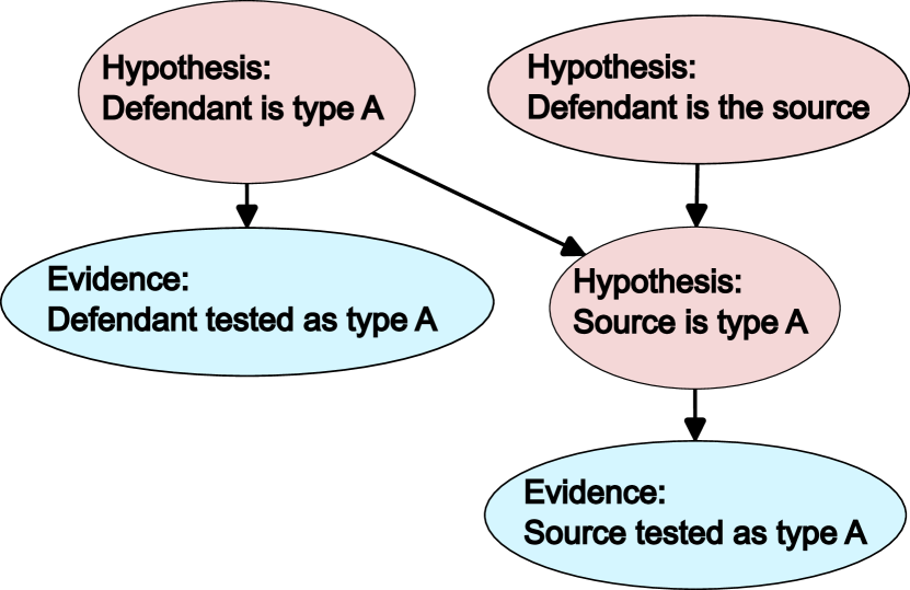
However, strictly speaking, three unknown hypotheses (“defendant is type A”, “defendant is the source”, “source is type A”) and two pieces of evidence (“defendant is tested as type A”, “source is tested as type A”) are involved in this seemingly simple analysis [114, 115] when we consider the potential errors from DNA collection and testing process [116, 117, 118]. Figure 3 (b) gives a complete causal link in this case, where pink nodes denote the hypotheses and blue nodes denote the observed evidence. To interpret the graph, we start from the prosecutor view hypothesis “the defendant is the source of the DNA found at the crime scene”. If meanwhile, the defendant has DNA type A, then we would expect the hypothesis “the source of DNA found at the crime scene is type A” to be true. Considering the possible errors, we can have the causal link from hypotheses “defendant is type A” and “source is type A” to the observed evidence “defendant tested as type A” and “source tested as type A” respectively.

Furthermore, there are other hidden hypotheses that we did not consider but related to the single piece of DNA evidence, for example, the hypothesis that the suspect was at the scene, etc. By using BN, we are able to study the relation between different types of evidence in a more thorough and complete way.

5.1 Object-oriented networks

Sometimes, problems may exhibit a hierarchical or repetitive structure that can be effectively modeled using Object-oriented Bayesian networks (OOBNs). In an OOBN, what may appear as a single node in the network can actually represent a network of its own. This hierarchical representation enhances the comprehensibility of the graph and facilitates modifications based on various scenarios and constraints [113, 119].

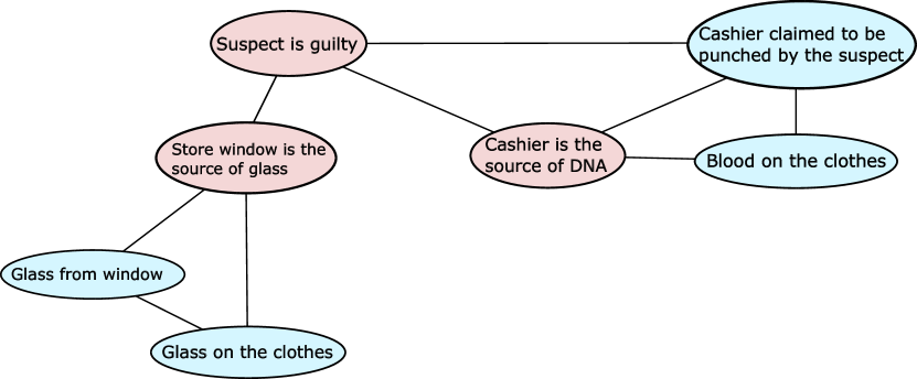
In [113], Dawid and Mortera made up a fictional crime. Here, we are going to study a simplified version to illustrate the use of OOBN. A male suspect broke into a convenience store at a gas station by smashing the window and punched the cashier in her face. When he was arrested, forensic laboratories took glass and blood samples from his clothing. The glass sample was indistinguishable from the glass at the store and the DNA obtained from the blood sample “matches” the cashier’s DNA type. We can construct a simple high-level graphical model as in Figure 4 to model the relationship of different pieces of evidence.

Figure 4: A simple example of generic modules in a high-level OOBN. This higher-order graph includes an unobserved identification module and three observed evidence modules witness, glass and DNA.

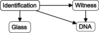
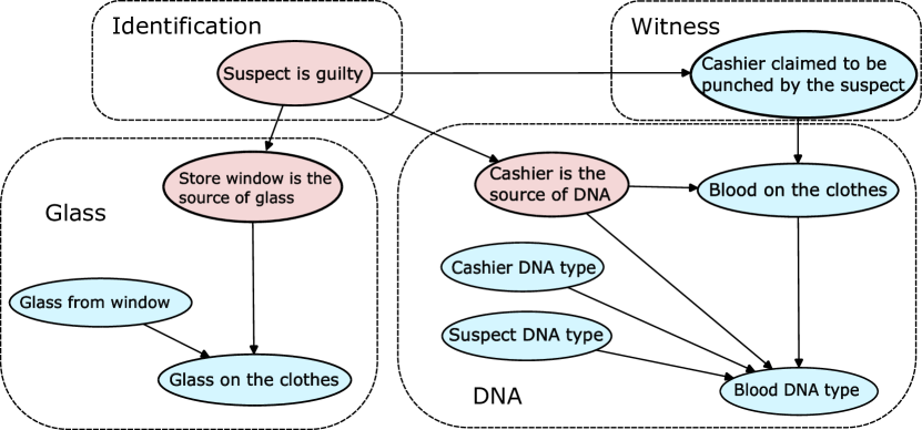
The graph consists of four modules, including an unobserved identification module and three observed evidence modules witness, glass, and DNA. Each module can be a DAG and the extended Bayesian network is shown in Figure 5 (a). Each dashed rectangle represents the sub-DAG of the corresponding higher-level module in Figure 4, where pink nodes represent unobserved hypotheses (Boolean) and blue nodes represent observed evidence. The identification module includes only one node: the prosecutor hypothesis “the suspect is guilty”. It will then lead to the hypotheses about the evidence “the store window is the source of glass retrieved from the suspect’s clothes” and “cashier is the source of the DNA retrieved from the blood on the suspect’s clothes”, as well as the witness’s testimony about “being punched by the suspect”. If the testimony is trustworthy and the cashier is indeed the source of the DNA, we would expect to see blood on the suspect’s clothes. To analyze the DNA samples obtained from the blood on suspect’s clothes, we need the blood sample, DNA profile from both cashier and suspect, and the hypothesis deciding if cashier is truly the source of the DNA. Similarly, if “the store window is the source of glass” is true, then together with the evidence “glass from the store window”, which is collected by the investigators after the crime, we should expect a match between the two glass samples.

(a) Expanded BN of the fictional crime

(b) “Moralised” graph

Figure 5: An expansion of the high-level Bayesian network (Figure 4) for the fictional crime. (a): Each dashed rectangle represents the sub-DAG of the corresponding higher-level module in Figure 4, where pink nodes represent unobserved hypotheses (Boolean) and blue nodes represent observed evidence. The identification module includes only one node: the prosecutor hypothesis “the suspect is guilty”. It will then lead to the hypotheses about the evidence “the store window is the source of glass retrieved from the suspect’s clothes” and “cashier is the source of the DNA retrieved from the blood on the suspect’s clothes”, as well as the witness’s testimony about “being punched by the suspect”. If the testimony is trustworthy and the cashier is indeed the source of the DNA, we would expect to see blood on the suspect’s clothes. To analyze the DNA samples obtained from the blood on suspect’s clothes, we need the blood sample, DNA profile from both cashier and suspect, and the hypothesis deciding if cashier is truly the source of the DNA. Similarly, if “the store window is the source of glass” is true, then together with the evidence “glass from the store window”, which is collected by the investigators after the crime, we should expect a match between the two glass samples. (b): Suppose we want to analyze the conditional independence between nodes “blood on the clothes” and “glass on the clothes”, we can use the “moralisation” method by selecting only the two nodes and their ancestors, “marry” all “unmarried” parents (“store window is the source of glass” and “glass from window”, “cashier claimed to be punched by the suspect” and “cashier is the source of DNA”) and drop the arrowheads. There is no path to connect the two nodes of interest while avoiding “suspect is guilty”, therefore conclude that given that we know if the suspect is guilty, the glass and DNA would not be affected by each other, thus two pieces of independent evidence.

OOBNs offer significant value through the utilization of generic network modules that can be reused, both within and across higher-level networks [120, 121, 122]. One example is the generic testimony model designed by Dawid, Hepler and Schum [123], based on witness credibility model by Schum and Morris [124] (shown in Figure 6 (a)).

(a) Generic testimony module

(b) sensation module

(c) accuracy module

Figure 6: Generic (a) testimony module, (b) sensation module, and (c) accuracy module [123]. The generic testimony module includes three stages: sensation (potential errors in the witness’s understanding of the event), objectivity (whether or not the witness’s perception accurately reflects the sensory evidence), and veracity (whether or not the witness honestly communicates the belief). The potential errors modeled by sensation comes from whether the real and perceived aspects of the event agree with each other (the agreement module) and the condition under which the observation is made (the “competent” node). The agreement, objectivity and veracity are all instances of the accuracy module, where a random error is used to determine if the output reproduces the input. Dotted nodes are inputs from outside the module.

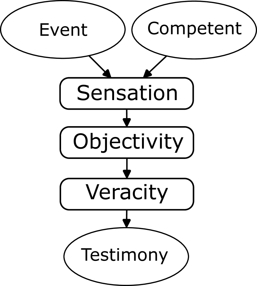
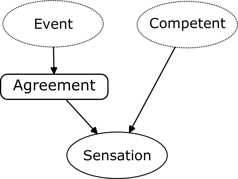
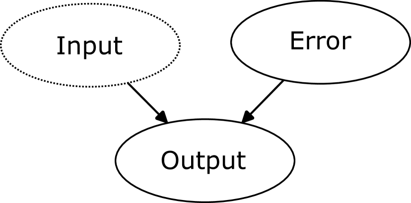
This model encompasses various aspects of eyewitness testimony regarding an event [124] and is organized into three distinct stages: sensation, objectivity, and veracity, which each of the stage itself can be a subgraph. Sensation models the potential of errors in the witness’s understanding of the event, which could result from their sensory and overall physical state (possibly causing disparities between the real and perceived aspects of the event, as denoted by agreement module in Figure 6 (b)), or from the situation under which the observation was made (the “competent” node in the graph). Figure 6 (b) is an instance of the sensation module along with the two input nodes “event” and “competent”, in which the agreement module is an instance of accuracy shown in Figure 6 (c), where a random error is used to determine if the output reproduces the input. The objectivity and veracity model whether or not the witness’s perception accurately reflects the sensory evidence and whether or not the witness honestly communicates the belief respectively, and they both are instances of the accuracy module.

Additionally, there are other generic modules available, such as identification, contradiction, corroboration, conflict, convergence, and explaining away, etc. [121]. These modules serve to enhance the versatility and applicability of OOBNs in different contexts.

5.2 Conditional independence

One of the most important concept in graphical models is conditional independence [125]. Similar to the definition of independent events, the conditional independence of two events $A$ and $B$ can be defined given a common condition, which is usually some background information or other available evidence $C$ in forensic science, as if the equality $\mathbb{P}(A,B|C)=\mathbb{P}(A|C)\cdot\mathbb{P}(B|C)$ holds, when $\mathbb{P}(C)>0$.

As a qualitative property, conditional independence does not involve numerical assessment, but it can sometimes impose the irrelevance of evidences, thus simplify the probability calculation (more details in Section 5.6). Steffen L. Lauritzen et al. [126] proposed a method to discover the hidden relationships called the “moralisation” criterion. To conclude the method, suppose we want to study the independence between $S$ and $T$ given $U$, we first form the ancestral graph, i.e., the subgraph of only $S$, $T$, $U$ and their ancestors. Then, add undirected links between any pairs of parents of a common child that have not yet connected and drop the arrows. This step is called “moralisation”. Finally, if there is no path that can connect $S$ and $T$ when avoiding $U$, we conclude the desired conditional independence.

An example is given in Figure 5 (b). Suppose we wish to examine the conditional independence between nodes labeled “Blood on the clothes” and “Glass on the clothes”, we can employ the “moralisation” method by selecting only these two nodes and their ancestors, “marry” all “unmarried” parents (“store window is the source of glass” and “glass from window”, “cashier claimed to be punched by the suspect” and “cashier is the source of DNA”) and drop the arrowheads, as shown in Figure 5 (b). There is no path to connect the two nodes of interests while avoiding “suspect is guilty”, therefore conclude that knowing the guilt or innocence of the suspect ensures that the evidence related to glass and DNA remains independent of each other. Similar results can be obtained from Figure 4, as the glass module and DNA module are conditionally independent given the identification module (no path to connect them while avoiding identification after dropping the arrowheads), and qualitatively speaking, they do not affect each other.

5.3 Quantitative analysis

Graphical models offer a simplified approach to assigning and manipulating probability distributions for variables. They enable the specification of conditional distributions for each node based on the states of its “parent” variables, eliminating the need to specify a vast collection of joint probabilities for all variables involved in the problem [113].

Let us take transfer probability as an example. Transfer probability is a crucial part of forensic statistics analysis, especially in the field of trace evidence and glass evidence. Curran et al. [127] proposed a Bayesian network model to study the transfer of glass fragments, which takes into account the transfer, persistence and recovery stages and attempts to study the dependence between them, based on the previous published studies [17]. Figure 7 gives a simplified graph.

Figure 7: A graphical model for the transfer of glass fragments [127]. This model takes into account: the number of fragments transferred to the breaker which is affected by the distance; the number of fragments that persist on the clothing which is affected by time and garment type; the number of fragments that can be retrieved which is affected by the persistent fragments and efficiency of the laboratory examination.

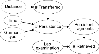
To be more specific, this model incorporates the effect of distance between the breaker and the window on the number of fragments transferred to the breaker; time and garment type on the number of fragments that persist on the clothing; and persistent fragments and efficiency of laboratory examination on the number of fragments retrieved. With this model, we can then compute marginal distribution of any variable or its conditional distribution given the data of some other observed specific variable [113]. This model is not definitive and relies on certain assumptions that may require further justification or refinement, but it is easy for examiners and researchers to enhance and modify based on their own cases and scenarios [7].

5.4 Forensic genetics

Bayesian networks are extremely widely used in the analysis of forensic genetics evidence, due to the nature of DNA that it is inherited from parents to children which is the natural causal link used to build BNs. Theoretical representation of such problems has been formulated as BNs [128] and as OOBNs [129].

5.4.1 Simple criminal cases

In a simple criminal case, we have two competing hypotheses regarding the DNA evidence found at the crime scene: $H_{\text{p}}$: the DNA trace belongs to the suspect and $H_{\text{d}}$: the DNA trace belongs to somebody else, i.e., the true offender. Figure 8 shows the expanded network of the OOBN, which consists of three modules: suspect, offender, and trace as well as the hypothesis “suspect is guilty?”.

Figure 8: Expanded network of OOBN for simple criminal case [130]. It includes three modules: suspect, offender, trace and the hypothesis “suspect is guilty?”. Both suspect and offender are instances of generic founder module, which consists of “paternal gene”, “maternal gene” and their unordered combination “genotype”. Module trace is an instance of generic identification module, where the “crime trace genotype” takes value of “suspect genotype” or “offender genotype” based on the true or false of the hypothesis respectively. Dotted nodes are inputs from outside the module.

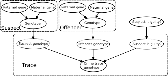
Modules suspect and offender are examples of the generic founder module, which consists of founding genes nodes “paternal gene”, “maternal gene” (assumed to be independently and identically drawn from specified allele frequencies for the corresponding marker) and their unordered combination “genotype” (because it is impossible to differentiate between the paternal gene and maternal gene within a genotype). For example, for marker D13, we may have $\mathbb{P}(\text{genotype}=\{9,14\}|\text{paternity gene}=9,\text{maternity gene}=14)=1$, where the paternity gene and maternity gene are drawn from the gene pool independently with corresponding allele frequencies. The trace module is an instance of the generic identification module, where the input comes from the suspect genotype and offender genotype, i.e., the output of corresponding modules. Node “crime trace genotype” is identical to “suspect genotype” or “offender genotype” given the true or false of the hypothesis “suspect is guilty?” respectively. To start the probability propagation, with the observed “suspect genotype” and “crime trace genotype”, we assign a prior probability (for example, 0.5) for the hypothesis “suspect is guilty?” to be true. The odds calculated for “suspect is guilty?” can then be considered the likelihood ratio supporting the prosecution’s hypothesis, based on the match at the corresponding marker. Assuming independence across markers, the overall likelihood ratio based on the full DNA evidence is obtained by multiplying these values across all markers [130, 113].

5.4.2 Simple paternity cases

In a simple paternity case, the network is usually built based on the observed DNA profiles of the mother, the child and the putative father. The goal is to find the likelihood ratio of the hypothesis of paternity $H_{\text{p}}$: the true father is the putative father against the non-paternity hypothesis $H_{\text{d}}$: the true father is an unspecified alternative father, who is unrelated to the putative father and is drawn from a reasonable subpopulation. The OOBN is shown in Figure 9 with generic founder modules mother, putative father, alternative father, generic identification module true father (both similar to those in simple criminal case), the hypothesis “putative father is the true father?”, and a generic child module to represent Mendelian inheritance at meiosis stage (also called meiosis module in some literatures), where the “child gene” is randomly drawn from either the maternal gene or paternal gene (denoted by the module fair coin flip).

Figure 9: OOBN for simple paternity case. The model consists of three generic founder modules mother, putative father, alternative father, a generic identification module true father, the hypothesis “putative father is the true father?”, and a generic child module, where the child’s gene is randomly drawn from either the maternal gene or the paternal gene modeled by a fair coin flip. Dotted nodes are inputs from outside of the module.

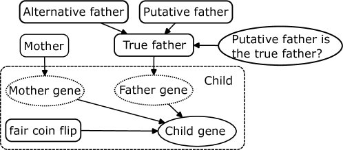
Similarly to the simple criminal case, we use the relevant allele frequency at each founder gene with the observed DNA data of mother, putative father and child and multiply the likelihood ratios for the overall LR.

5.4.3 Complex cases

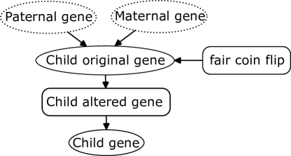
One significant benefit of OOBN representations is their capability to easily expand the network by incorporating additional features [129]. For example, we can modify the network to allow for mutation, by formulating and integrating different mutation models [131, 132]. Such alternations are usually limited to low-level networks, whereas the other modules and the overall high-level structure remain unaltered. In practice, we can make distinction between an original gene, which is an exact copy of one of the parents’ genes, and the potentially modified gene due to the mutation. Let us consider the generic child module in Figure 9. Dawid et al. introduced the modified generic module mutation to model the mutation of meiosis stage, which applies statistical mutation models on “child original gene” node, that gives an output of observed “child gene” after potential mutation happened in the meiosis stage. The modified module is shown in Figure 10.

Figure 10: Modified child module while considering potential mutation that happens during the meiosis stage in the cells [129]. Instead of having the “child gene” identical to either paternal gene or maternal gene, a generic mutation module is used to apply statistical mutation models on “child original gene” so that we get the output of observed “child gene” after potential mutation.

Another benefit lies in the capacity of employ existing network modules in novel combinations, enabling the creation of unique narratives. For example, consider a more complicated paternity case, where the DNA profile of the putative father is unavailable, but is available from one of his siblings. Figure 11 gives a modified network from Figure 9.

Figure 11: OOBN for a complex paternity case where DNA profile of putative father is unavailable [113]. Grandfather, grandmother, alternative father and mother are instances of generic founder module. Putative father (unlike in Figure 9), sibling and child are instances of generic child (or meiosis) module. We can then connect the putative father node and the sibling node through their common parents, the grandfather node and grandmother node.

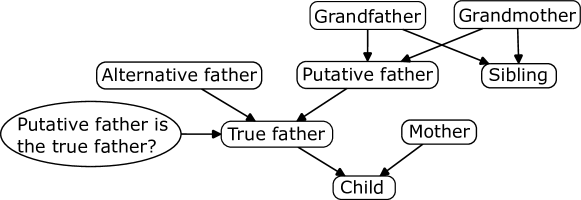
In this case, we only have the DNA profile of the child, the mother, and the putative father’s sibling. The generic founder modules include grandfather, grandmother, alternative father and mother; the generic child modules include putative father, sibling and child. We can then connect the putative father node and the sibling node through their common parents, the grandfather node and grandmother node. The rest of the graph would be the same as Figure 9. To accommodate more complicated cases, we can similarly add or edit different modules for each specific case, without changing the structure within each node, therefore provide a clearer and simpler point of view for complex cases.

5.4.4 DNA mixture

Bayesian networks is a powerful tool when analyzing DNA mixtures. Assume the mixture contains DNA from two individuals, we are interested in the two competing hypotheses: $H_{\text{p}}$: the victim and the suspect contributed to the mixture versus $H_{\text{d}}$: the victim and an unknown individual (unknown individual 1) contributed to the mixture. Alternatively, for cases where the victim is not the main source of the DNA sample, we might consider another unknown individual instead of the victim, and therefore the hypotheses would be: $H_{\text{p}^{\prime}}$: the suspect and an unknown individual (unknown individual 2) contributed to the mixture versus $H_{\text{d}^{\prime}}$: two unknown contributors (unknown individual 1 and 2) contributed to the mixture. Figure 12 shows an OOBN of this case.

Figure 12: OOBN for a two-contributor DNA mixture. Taking from the evidence we use an example in which we observe only three alleles (A, B, and C) and no other alleles from the evidence collected, each has a corresponding node on the top. The true or false of these four nodes depends on genotype of both individual 1 and individual 2, the two contributors in this case, which are instances of generic identification module, as they take value of “suspect/unknown individual 1 genotype” (generic founder module) and “victim/unknown individual 2 genotype” (generic founder module) respectively based on the true or false of the corresponding hypothesis “individual 1 is suspect?” and “individual 2 is victim?”. This graph can let us calculate the likelihood of the four logical combinations of the two hypotheses.

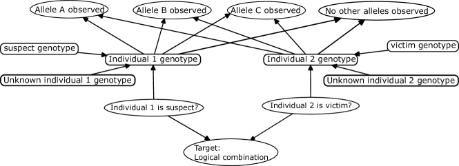
Suppose we observe three alleles (A, B, and C) and no other alleles at the marker from the evidence collected, we have the four nodes at the top of the graph. We can easily adjust the network to accommodate varying numbers of alleles. The true or false of these four nodes depends on genotype of both individual 1 and individual 2, the two contributors in this case, which are instances of generic identification module, as they take value of “suspect/unknown individual 1 genotype” (generic founder module) and “victim/unknown individual 2 genotype” (generic founder module) respectively based on the true or false of the corresponding hypothesis “individual 1 is suspect?” and “individual 2 is victim?”. Both “suspect genotype” and “victim genotype” are observed. The target of this graph is to calculate the likelihood of the four logical combinations of the two hypotheses, namely, the two contributors are: 1) suspect and victim; 2) suspect and an unknown individual; 3) an unknown individual and victim; 4) two unknown individuals. Similar to previous sections, we can use modules to account for potential mutation and issues such as allele drop-out. Furthermore, Mortera et al. introduced nodes for the number of unknown contributors, and the total number of contributors, as in most cases the number of contributors itself is uncertain [133].

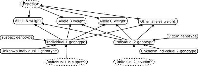
Peak heights or peak areas can still be used in quantitative analysis. Since the proportion of DNA contributed by each individual is constant across all the markers, we can use a common “fraction” module to connect all the markers we want to analyze, each of them is a generic marker module shown in Figure 13, which is an extension of Figure 12 with additional information of fraction of peak height [134, 113]. We use a common “fraction” node and a common target module to connect all markers of interests. Within each generic marker module, we have the same structure as shown in Figure 12, while only changing the four evidence nodes into modules which model the quantitative information on peak height.

Figure 13: Marker module for DNA mixture with peak height information [134]. We use a common “fraction” node and a common target module (the hypotheses) to connect all markers of interests. Within each generic marker module, instead of having four evidence nodes, we use modules which model the quantitative information on peak height. Dotted nodes are from outside the module.

5.4.5 Assumptions on founder genes

The conventional assumptions of fixed and known allele frequencies, independence among individuals in the model, and homogeneity in the allele frequency database can all be subject to scrutiny [130]. In practice, the allele frequencies (for example, the “paternity gene” and “maternity gene” nodes in Figure 8) used for probabilistic forensic inference are not known probabilities but rather estimates derived from empirical frequencies in a database. Green and Mortera [130] introduced a Bayesian model to simulate the uncertainty in allele frequency, with a Dirichlet prior and multinomial sampling, resulting in a posterior Dirichlet distribution. Specifically, for simplicity we consider only one marker at a time, suppose $X_{1},\ldots,X_{N}$ is the database of interests, which are random samples drawn from the corresponding population with sample size of $N$ subjects. Suppose there are $K$ possible allele types at this marker, and we denote the number (or absolute frequency) of type $j$ alleles of this marker being drawn as $(Y_{1},\ldots,Y_{K})$, where

$$Y_{j}=\sum_{i=1}^{N}\mathbbm{1}\{X_{i}=\text{type }j\}$$ (19)

and

$$(Y_{1},\ldots,Y_{K})\sim\text{Multinomial}(N,r_{1},\ldots,r_{K})~{}\text{with}~{}r_{i}\in[0,1],\forall i,~{}\text{and}~{}\sum_{j=1}^{K}r_{j}=1.$$ (20)

Note that $\sum_{j=1}^{K}Y_{j}=N$. For the probability parameters $\{r_{1},\ldots,r_{K}\}$, we put a Dirichlet prior on them, that is,

$$(r_{1},\ldots,r_{K})\sim\text{Dirichlet}(\alpha_{1},\ldots,\alpha_{K}),~{}\text{where}~{}\alpha_{j}>0,~{}j=1,\ldots,K.$$ (21)

Since Dirichlet distribution is the conjugate prior for multinomial likelihood, the posterior distribution is given by

$$(r_{1},\ldots,r_{K})|(Y_{1},\ldots,Y_{K})\sim\text{Dirichlet}(\alpha_{1}+Y_{1},\ldots,\alpha_{K}+Y_{K}).$$ (22)

By letting $M=\sum_{j=1}^{K}(\alpha_{j}+Y_{j})=N+\sum_{j=1}^{K}\alpha_{j}$ be the sum of the posterior parameters, the posterior distribution can be rewritten as

$$(r_{1},\ldots,r_{K})|(Y_{1},\ldots,Y_{K})\sim\text{Dirichlet}(M\rho_{1},\ldots,M\rho_{K}),$$ (23)

where

$$\rho_{j}=\frac{\alpha_{j}+Y_{j}}{M}$$ (24)

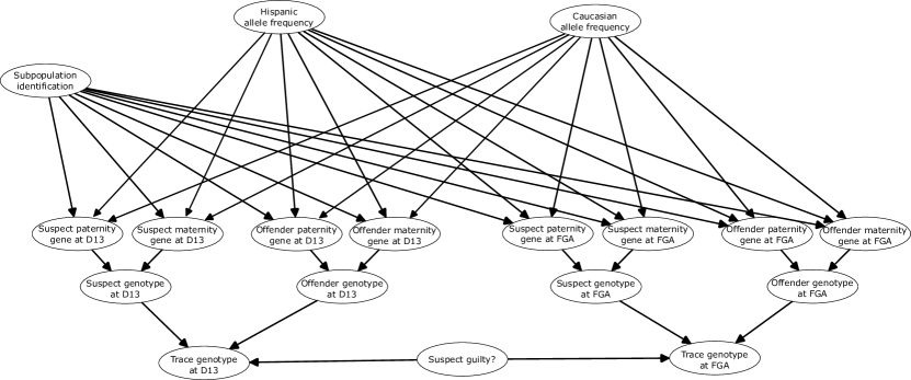
is the posterior mean of $r_{j}|(Y_{1},\ldots,Y_{K})$, that is, the database allele relative frequency. The founding genes are drawn conditionally independently and identically from this posterior Dirichlet distribution, which corresponds to the standard set-up of a Dirichlet process [135] and can be represented as a Bayesian network using Pólya urn scheme [136]. Figure 14 shows a graphical model of the sampling process modified from the simple criminal case illustrated in Section 5.4.1, where we have four founding genes, namely suspect paternity, suspect maternity, offender paternity and offender maternity. Due to the exchangeability of Pólya urn scheme [137], the order of the four founding genes being sampled does not affect the results. Therefore we will call the four unordered founding genes $g_{1}$, $g_{2}$, $g_{3}$ and $g_{4}$ for simplicity in Figure 14.

Figure 14: Network for Pólya urn scheme. We first draw $g_{1}$ randomly from gene pool based on the database allele relative frequency $\vec{\rho}$. For $g_{2}$, with probability $\frac{1}{M+1}$, it is set to be the same type as $g_{1}$, and otherwise (with probability $\frac{M}{M+1}$) is randomly drawn from the gene pool. For founding gene $g_{n}$, it has probability $\frac{1}{M+n-1}$ each to be equal to each of $g_{1},g_{2},\ldots,g_{n-1}$, and with the remaining probability $\frac{M}{M+n-1}$ to be drawn randomly from the gene pool.

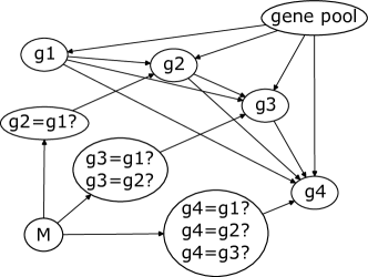
We first draw $g_{1}$ randomly from gene pool based on the database allele relative frequency $\vec{\rho}$, that is, $g_{1}$ has probability $\rho_{j}$ to be allele type $j$. For $g_{2}$, with probability $\frac{1}{M+1}$, it is set to be the same type as $g_{1}$, and otherwise (with probability $\frac{M}{M+1}$) is randomly drawn from the gene pool similarly to $g_{1}$. For $g_{3}$, it has probability $\frac{1}{M+2}$ to be equal to $g_{1}$, probability $\frac{1}{M+2}$ to be equal to $g_{2}$, and probability $\frac{M}{M+2}$ to be randomly drawn from the gene pool. Similarly, for founding gene $g_{n}$, it has probability $\frac{1}{M+n-1}$ each to be equal to each of $g_{1},g_{2},\ldots,g_{n-1}$, and with the remaining probability $\frac{M}{M+n-1}$ to be drawn randomly directly from the gene pool. A modified network can be designed so that all choices are binary to save computational time and space in probability propagation [138]. This module can be utilized in a higher-level network to compute inferences, for example, we can change the four founding genes nodes in Figure 8 as $g_{1},\ldots,g_{4}$ from Figure 14.

The assumption of a homogeneous DNA reference population is also questionable as populations often comprise diverse subgroups. The sensitivity analysis concerning founder genes is also influenced by the choice of relevant population and corresponding allele frequency database, leading to potential variations in results. The uncertainty regarding the relevant population can also induce dependence between actors, observed or unobserved, and induce marker dependence in cases involving untyped individuals. A solution would be drawing the founder genes from corresponding subpopulation allele frequencies. Figure 15 gives a Bayesian network to demonstrate this process. For simplicity, we consider only two subpopulation (Hispanic and Caucasian) and two genetic markers (D13 and FGA). The node “subpopulation indication” decides whether the founder genes (suspect paternity, suspect maternity, offender paternity and offender maternity) are drawn from which subpopulation and it should be the same for each actor. The suspect/offender and corresponding paternity/maternity gene form the generic founder module as mentioned in Section 5.4.1. Whether the trace genotype at D13 and FGA take values from suspect/offender genetypes depends on the “suspect guilty” node.

Figure 15: Bayesian network when considering subpopulations. For simplicity, we consider only two subpopulation (Hispanic and Caucasian) and two genetic markers (D13 and FGA). The node “subpopulation indication” decides whether the founder genes (suspect paternity, suspect maternity, offender paternity and offender maternity) are drawn from which subpopulation and it should be the same for each actor. The suspect/offender and corresponding paternity/maternity gene form the generic founder module as mentioned in Section 5.4.1. Whether the trace genotype at D13 and FGA take values from suspect/offender genetypes depends on the “suspect guilty” node.

5.5 Chain event graph (CEG)

Chain event graph (CEG) is used to represent and analyze causal hypotheses in domains with discrete, asymmetric, and context-specific information, where the measurement variables can exhibit varying sets of potential outcomes based on different combinations of values for sets of ancestral variables [139, 140, 141, 142, 143, 144, 145]. Briefly speaking, a CEG is a function of an event tree [146], which is a directed, rooted tree with vertex set and edge set. The non-leaf vertices are called situations and are the indices of random variables that characterize the subsequent stages of potential developments in the unfolding process. The path from the root to the leaves represent events and provide labels for the various potential developments of the described process. Smith and Anderson introduced an inclusive definition of CEG [147].

Thwaites et al. made an example of CEG [148]. Here we simplify the example just as a demonstration. The police have detained a suspect they believe threw a brick through a shop window. While they aim to take him to court, there might be reasons hindering the proceedings. Similar to building decision trees for dicision analysis [149], a CEG is shown in Figure 16.

Figure 16: Chain Event Graph example. The first indicator on the left side is whether to proceed the case or not. Whether the suspect broke the glass does not depend on whether the case was proceeded or not, and if the police decides to proceed, the glass evidence would be sent to the forensic laboratory and therefore the next indicator would be whether the glass evidence match. If the glass evidence does not match, or if the police decides not to proceed, the graph will lead to the indicator of releasing the suspect. Otherwise, if the glass evidence match, the suspect would be brought to trial.

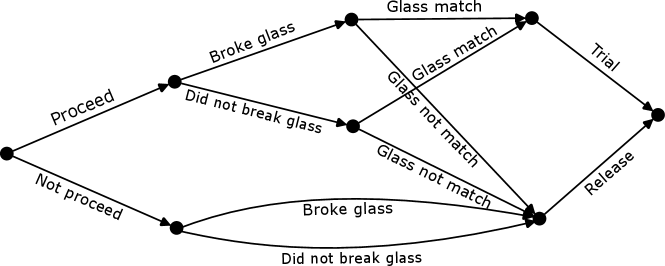
The chain event graph was constructed in temporal order. The first indicator on the left side is whether to proceed the case or not. Whether the suspect broke the glass does not depend on whether the case was proceeded or not, and if the police decides to proceed, the glass evidence would be sent to the forensic laboratory and therefore the next indicator would be whether the glass evidence match. If the glass evidence does not match, or if the police decides not to proceed, the graph will lead to the indicator of releasing the suspect. Otherwise, if the glass evidence match, the suspect would be brought to trial. Therefore, probability propagation can be conducted and conditional independence can be analyzed.

5.6 Compute posterior distributions in DAGs

In Bayesian networks used for forensic science, specific variables within the graphs are assigned predetermined values and/or probabilities based on previous studies, for example, the population frequency of an allele. Our objective is to determine the posterior distribution of other variables of interest by marginalizing across the joint distribution, which can be costly. Belief propagation is a local message-passing type algorithm for the computation but is confined to tree structures [150, 151, 152]. The basic idea involves treating each variable as a simple processor and examining asynchronous local message passing among different nodes until equilibrium is attained.

Suppose $X$ is the node of interest and $E$ is any subset of observed nodes with predetermined values. Furthermore, let $E=E_{X}^{+}\cup E_{X}^{-}$, where $E_{X}^{+}$ are the ancestor nodes of $X$ and $E_{X}^{-}$ are descendant nodes of $X$. We then have

$$p(x|e_{X}^{+},e_{X}^{-})=\mathbb{P}(X=x|E_{X}^{+}=e_{X}^{+},E_{X}^{-}=e_{X}^{-})\propto m^{+}(x)m^{-}(x),$$ (25)

where $m^{+}(x)=p(x|e_{X}^{+})$ is the summary message passed to $X$ from all of its ancestors and $m^{-}(x)=p(e_{X}^{-}|x)$ is the summary message passed to $X$ from all of its descendants. Without loss of generality, we assume $X$ has $k$ parents (denoted as $Z_{1},\ldots,Z_{k}$) and $n$ children (denoted by $Y_{1},\ldots,Y_{n}$). The message $m^{+}(x)$ captures the belief about the values of the parents, and is similar to the “prior” probabilities. In contrast, the message $m^{-}(x)$ incorporates information from the children that are pertinent to the belief of the value of the parent $X$, resembling the “likelihood” term for the application of Bayes rule. Therefore, Equation 25 can be viewed as the multiplication of prior message and the likelihood message, just like the factorization in Bayesian statistics.

To determine Equation 25, computation of the summary messages from both parents and children of $X$ is necessary. The calculation of the message from children (“likelihood” message) is simple, as the children $Y_{1},\ldots,Y_{n}$ are conditionally independent given $X$. Therefore,

$$m^{-}(x)=\prod_{j=1}^{n}m_{Y_{j}}^{-}(x),$$ (26)

i.e., the summary message from the children is the product of individual messages from each child of the node. The computing of the summary message from parents (“prior” message) is a bit more intricate, yet it can still be derived following the probability rules. We have

$$m^{+}(x)=\sum_{z_{1}}\cdots\sum_{z_{k}}p(x|z_{1},\ldots,z_{k})\prod_{i=1}^{k}m_{X}^{+}(z_{i}),$$ (27)

i.e., we obtain the joint probability of the child and all the parents by multiplying the joint prior probability of the parent nodes ($\prod_{i=1}^{k}m_{X}^{+}(z_{i})$ assuming that the parents are independent from each other) by the conditional probability of $X$ given all of the parents, then marginalize out all the parent nodes.

The next step would be to compute the individual messages from each parent and each child of $X$. To compute the individual message from a parent node $Z_{i}$ to $X$, we first need to find the summary message from all parent nodes of $Z_{i}$, as well as the individual messages from all the children of $Z_{i}$ except $X$, then pass it to $X$. Suppose $\{X,X_{1},\ldots,X_{l}\}$ is the set of all the children of $Z_{i}$, we have

$$m_{X}^{+}(z_{i})=m^{+}(z_{i})\prod_{X_{a}\in\{X_{1},\ldots,X_{l}\}}m_{X_{a}}^{-}(z_{i}).$$ (28)

Similarly, for individual messages from a child $Y_{j}$ to $X$, we first need to obtain the summary message from all child nodes of $Y_{j}$, as well as the individual messages from all the parents of $Y_{j}$ except $X$, then pass it to $X$. Suppose $\{X,X_{1},\ldots,X_{q}\}$ is the set of all the parents of $Y_{j}$, we have

$$m_{Y_{j}}^{-}(X)=\sum_{y_{j}}m^{-}(y_{j})\sum_{\{x_{1},\ldots,x_{q}\}}p(y_{j}|x,x_{1},\ldots,x_{q})\prod_{x_{b}\in\{x_{1},\ldots,x_{q}\}}m_{Y_{j}}^{+}(x_{b}).$$ (29)

Exact inference, as introduced earlier, may face challenges in certain scenarios. If the underlying undirected graph contains cycles, the belief propagation algorithm no longer works, as the ancestors and descendants of $X$ are not guaranteed to be independent given $X$. To address this, we need to transform the graph into a polytree, in which some nodes may represent a set of original variables. Additionally, exact inference becomes infeasible in the presence of large cliques or extended loops. While belief propagation can sometimes be directly applied to graphs with loops, its convergence is not guaranteed [153]. Other common approaches for approximate inference include variational methods and sampling methods.

6 Conclusion

In conclusion, statistics plays a crucial role in forensic science, particularly in the analysis, interpretation, and reporting of evidence. Following the 2009 National Research Council report Strengthening Forensic Science in the United States: A Path Forward, which underscored the importance of establishing national-level standards concerning issues related to statistics, we reviewed the challenges of promoting statistics in court. The difficulties in promoting statistics in court are multifaceted, spanning from the complexities of statistical models, such as computational intricacies, to challenges arising from the subjective nature of evidence examiners, including cognitive biases, and extending to the broader audience, where lay individuals struggle with limited understanding of statistical concepts.

One of the most important statistical frameworks used in forensic evidence evaluation is the likelihood ratio framework. This framework allows forensic scientists to calculate the likelihood of observing a particular piece of evidence from the prosecutor propositions versus the defense hypotheses. We reviewed the evolution of verbal interpretation of likelihood concurrently with the rapid advancements in evidence identification technology, particularly in the field of DNA typing, where the likelihood ratio can be used to determine the strength of the evidence linking a suspect to a crime. Likelihood ratio framework also demonstrates its efficiency in handling complicated scenarios, such as co-ancestry assumptions and DNA mixtures. However, challenges arise in constructing likelihood ratios for various types of evidence, notably due to the absence of prior knowledge regarding the population distribution of evidence, particularly in cases involving pattern evidence such as fingerprints.

Graphical models, particularly directed acyclic graphs, prove to be a valuable tool for illustrating the connections between hypotheses and different pieces of evidence, as well as the causal links between information. Object-oriented networks, functioning at a higher level, offer simplicity and the ability to generalize certain structure across different case scenarios. Graphical models are beneficial for DNA typing, enabling the clear and logical representation of both criminal and paternity cases, whether simple or complex, as well as DNA mixtures and assumptions on founder genes. For asymmetric structures, a chain event graph serves as a suitable representation of events occurring in a case.

In essence, the use of statistics in forensic science is pivotal for ensuring justice. Advancements of statistical techniques for evidence assessment are crucial, aiming to enhance the accuracy and dependability of forensic investigations. This continuous improvement holds the promise of delivering more just outcomes within the criminal justice system.

References

- [1] Samuel R Gross. Convicting the innocent. Annual review of law and social science, 4:173–192, 2008.
- [2] The University of California Irvine Newkirk Center for Science & Society, University of Michigan Law School, and Michigan State University College of Law. The national registry of exonerations 2022 annual report, May 2023.
- [3] California Courts. Types of cases, 2023.
- [4] Middle District of Florida. Civil or criminal?
- [5] The Committee on the Judiciary House of Representatives. Federal rules of criminal procedure.
- [6] Offices of the United States Attorneys. Steps in the federal criminal process.
- [7] James M Curran. Statistics in forensic science. Wiley Interdisciplinary Reviews: Computational Statistics, 1(2):141–156, 2009.
- [8] National Research Council et al. Strengthening forensic science in the United States: a path forward. National Academies Press, 2009.
- [9] Elizabeth D Schafer. Ancient science and forensics. Forensic Science, 1:41–45, 2008.
- [10] Daniel Asen. Song ci (1186–1249), father of world legal medicine: history, science, and forensic culture in contemporary china. East Asian Science, Technology and Society: An International Journal, 11(2):185–207, 2017.
- [11] Douglas Harper et al. Online etymology dictionary, 2001.
- [12] MM Houck. 19th interpol international forensic science managers symposium, 2019.
- [13] Craig Adam. Essential mathematics and statistics for forensic science. John Wiley & Sons, 2011.
- [14] Barry AJ Fisher, William J Tilstone, and Catherine Woytowicz. Introduction to criminalistics: the foundation of forensic science. Academic Press, 2009.
- [15] Richard Saferstein. Criminalistics: An introduction to forensic science. Prentice Hall New Jersey, 2004.
- [16] James M Curran. The statistical interpretation of forensic glass evidence. International Statistical Review, 71(3):497–520, 2003.
- [17] James Michael Curran, Tacha Natalie Hicks Champod, and John S Buckleton. Forensic interpretation of glass evidence. CRC Press, 2000.
- [18] SM Ojena and PR De Forest. Precise refractive index determination by the immersion method, using phase contrast microscopy and the mettler hot stage. Journal of the Forensic Science Society, 12(1):315–329, 1972.
- [19] New Scotland Yard. Fingerprint history: A synopsis of the development of the system of fingerprint identification with particular reference to new scotland yard. Metropolitan Police, New Scotland Yard, London, 1990.
- [20] Colin Beavan. Fingerprints: The Origins of Crime Dectection and the Murder Case That Launched Forensic Science. Hyperion Books, 2002.
- [21] Gerald Lambourne. The fingerprint story. Harrap, 1984.
- [22] Jeffery G. Barnes. Fingerprint sourcebook-chapter 1: History. US Dept. of Justice, Office of Justice Programs, National Institute of Justice, 2010.
- [23] Anil Jain, Yi Chen, and Meltem Demirkus. Pores and ridges: Fingerprint matching using level 3 features. In 18th International Conference on Pattern Recognition (ICPR’06), volume 4, pages 477–480. IEEE, 2006.
- [24] David R Ashbaugh. Quantitative-qualitative friction ridge analysis: an introduction to basic and advanced ridgeology. CRC press, 1999.
- [25] Sharath Pankanti, Salil Prabhakar, and Anil K Jain. On the individuality of fingerprints. IEEE Transactions on pattern analysis and machine intelligence, 24(8):1010–1025, 2002.
- [26] Jonathan D Stosz and Lisa A Alyea. Automated system for fingerprint authentication using pores and ridge structure. In Automatic systems for the identification and inspection of humans, volume 2277, pages 210–223. SPIE, 1994.
- [27] Francis Galton. Finger prints. Macmillan and Company, 1892. 57490-57492.
- [28] Erin Murphy. Forensic dna typing. Annual review of criminology, 1:497–515, 2018.
- [29] The United States Department of Justice. Advancing justice through dna technology: Using dna to solve crimes, Mar 2017.
- [30] Paul Johnson and Robin Williams. Post-conviction dna testing: the uk’s first ‘exoneration’case? Science & justice: journal of the Forensic Science Society, 44(2):77, 2004.
- [31] John M Butler. Forensic DNA typing: biology, technology, and genetics of STR markers. Elsevier, 2005.
- [32] Federal Bureau of Investigation. Combined dna index system (codis): Codis information for law enforcement, 2018.
- [33] Efthymia Karantzali, Phaedra Rosmaraki, Anastasios Kotsakis, Marie-Gaëlle Le Roux-Le Pajolec, and Georgios Fitsialos. The effect of fbi codis core str loci expansion on familial dna database searching. Forensic Science International: Genetics, 43:102129, 2019.
- [34] John S Buckleton, James M Curran, and Peter Gill. Towards understanding the effect of uncertainty in the number of contributors to dna stains. Forensic Science International: Genetics, 1(1):20–28, 2007.
- [35] Simson L Garfinkel. Digital forensics research: The next 10 years. digital investigation, 7:S64–S73, 2010.
- [36] André Årnes. Digital forensics. John Wiley & Sons, 2017.
- [37] Joseph L Gastwirth. Statistical science in the courtroom. Springer Science & Business Media, 2012.
- [38] Joseph B Kadane. Statistics in the Law: A Practitioner’s Guide, Cases, and Materials. Oxford University Press, 2008.
- [39] Jonathan J Koehler. Probabilities in the courtroom: An evaluation of the objections and policies. Handbook of psychology and law, pages 167–184, 1992.
- [40] Ted Vosk and Ashley F Emery. Forensic metrology: Scientific measurement and inference for lawyers, judges, and criminalists. CRC Press, 2014.
- [41] Norman Fenton, Martin Neil, and Daniel Berger. Bayes and the law. Annual review of statistics and its application, 3:51–77, 2016.
- [42] Paul Meier and Sandy Zabell. Benjamin peirce and the howland will. Journal of the American Statistical Association, 75(371):497–506, 1980.
- [43] Simon A Cole and Matt Barno. Probabilistic reporting in criminal cases in the united states: A baseline study. Science & justice: journal of the Forensic Science Society, 60(5):406–414, 2020.
- [44] Roberto Puch-Solis, Paul Roberts, Susan Pope, and Colin Aitken. Assessing the probative value of dna evidence. Guidance for Judges, Lawyers, Forensic Scientists and Expert Witnesses, Practitioner Guide, 2, 2012.
- [45] Graham Jackson, Colin Aitken, and Paul Roberts. Case assessment and interpretation of expert evidence. Guidance for judges, lawyers, forensic scientists and expert witnesses. Practitioner guide, 4:145, 2015.
- [46] Geoffrey Stewart Morrison. Advancing a paradigm shift in evaluation of forensic evidence: The rise of forensic data science. Forensic Science International: Synergy, page 100270, 2022.
- [47] A Oig. Review of the fbi’s handling of the brandon mayfield case. Office of the Inspector General, Oversight and Review Division, US Department of Justice, pages 1–330, 2006.
- [48] Eric Lichtblau. Us will pay $2 million to lawyer wrongly jailed. New York Times, 30(11), 2006.
- [49] Itiel E Dror, David Charlton, and Ailsa E Péron. Contextual information renders experts vulnerable to making erroneous identifications. Forensic science international, 156(1):74–78, 2006.
- [50] Jonathan J Koehler. One in millions, billions, and trillions: Lessons from people v. collins (1968) for people v. simpson (1995). J. Legal Educ., 47:214, 1997.
- [51] Norman Fenton, Daniel Berger, David Lagnado, Martin Neil, and Anne Hsu. When ‘neutral’evidence still has probative value (with implications from the barry george case). Science & Justice, 54(4):274–287, 2014.
- [52] Ronald Meester, Marieke Collins, Richard Gill, and Michiel Van Lambalgen. On the (ab) use of statistics in the legal case against the nurse lucia de b. Law, Probability & Risk, 5(3-4):233–250, 2006.
- [53] Roger W Byard. Unexpected infant death: lessons from the sally clark case. Medical journal of Australia, 181(1):52–54, 2004.
- [54] Richard Nobles and David Schiff. Misleading statistics within criminal trials: The sally clark case. Significance, 2(1):17–19, 2005.
- [55] A Philip Dawid. Bayes’s theorem and weighing evidence by juries. In PROCEEDINGS-BRITISH ACADEMY, volume 113, pages 71–90. Citeseer, 2002.
- [56] Ray Hill. Multiple sudden infant deaths–coincidence or beyond coincidence? Paediatric and perinatal epidemiology, 18(5):320–326, 2004.
- [57] Learned Hand. Historical and practical considerations regarding expert testimony. Harvard Law Review, pages 40–58, 1901.
- [58] Graham Jackson, Stella Jones, Gareth Booth, Christophe Champod, and Ian W Evett. The nature of forensic science opinion–a possible framework to guide thinking and practice in investigations and in court proceedings. Science & justice: journal of the Forensic Science Society, 46(1):33–44, 2006.
- [59] Harry Collins and Robert Evans. Rethinking expertise. University of Chicago Press, 2019.
- [60] Gary Edmond, Bryan Found, Kristy Martire, Kaye Ballantyne, David Hamer, Rachel Searston, Matthew Thompson, Emma Cunliffe, Richard Kemp, Mehera San Roque, et al. Model forensic science. Australian Journal of Forensic Sciences, 48(5):496–537, 2016.
- [61] Kristy A Martire and Gary Edmond. How well do lay people comprehend statistical statements from forensic scientists? In Handbook of Forensic Statistics, pages 201–224. Chapman and Hall/CRC, 2020.
- [62] David L Faigman and AJ Baglioni Jr. Bayes’ theorem in the trial process: Instructing jurors on the value of statistical evidence. Law and Human Behavior, 12(1):1–17, 1988.
- [63] Peter Tillers, Eric D Green, et al. Probability and Inference in the Law of Evidence: the uses and limits of Bayesianism. Springer, 1988.
- [64] Stephen E Fienberg and Michael O Finkelstein. Bayesian statistics and the law. Bayesian statistics, 5:129–146, 1996.
- [65] Stephen E Fienberg. Bayesian models and methods in public policy and government settings. Statistical Science, 26(2):212–226, 2011.
- [66] Roger Cook, Ian W Evett, Graham Jackson, PJ Jones, and JA Lambert. A hierarchy of propositions: deciding which level to address in casework. Science & Justice, 38(4):231–239, 1998.
- [67] Ian W Evett. Bayesian inference and forensic science: problems and perspectives. Journal of the Royal Statistical Society. Series D (The Statistician), 36(2/3):99–105, 1987.
- [68] Harold Jeffreys. The theory of probability. OuP Oxford, 1998.
- [69] Ian W Evett. Towards a uniform framework for reporting opinions in forensic science casework. Science & Justice, 3(38):198–202, 1998.
- [70] Ian W Evett, Graham Jackson, JA Lambert, and S McCrossan. The impact of the principles of evidence interpretation on the structure and content of statements. Science & justice: journal of the Forensic Science Society, 40(4):233–239, 2000.
- [71] Kristy A Martire, Richard I Kemp, M Sayle, and Ben R Newell. On the interpretation of likelihood ratios in forensic science evidence: Presentation formats and the weak evidence effect. Forensic science international, 240:61–68, 2014.
- [72] Raymond Marquis, Alex Biedermann, Liv Cadola, Christophe Champod, Line Gueissaz, Geneviève Massonnet, Williams David Mazzella, Franco Taroni, and Tacha Hicks. Discussion on how to implement a verbal scale in a forensic laboratory: Benefits, pitfalls and suggestions to avoid misunderstandings. Science & Justice, 56(5):364–370, 2016.
- [73] Hal S Stern. Statistical issues in forensic science. Annual Review of Statistics and Its Application, 4:225–244, 2017.
- [74] John S Buckleton, Christopher M Triggs, Simon J Walsh, et al. Forensic dna evidence interpretation. Technical report, CRC Press, 2005.
- [75] Charles William Cotterman. A calculus for statistico-genetics. PhD thesis, The Ohio State University, 1940.
- [76] Gustave Malécot. Les mathématiques de l’hérédité. Paris: masson et Cie, 1948.
- [77] CC Li and Louis Sacks. The derivation of joint distribution and correlation between relatives by the use of stochastic matrices. Biometrics, 10(3):347–360, 1954.
- [78] Albert Jacquard. Genetic information given by a relative. Biometrics, pages 1101–1114, 1972.
- [79] National Research Council et al. National research council committee on dna forensic science. the evaluation of forensic dna evidence: an update, 1996.
- [80] David J Balding and Christopher D Steele. Weight-of-evidence for Forensic DNA Profiles. John Wiley & Sons, 2015.
- [81] Bruce Budowle, Tamyra R Moretti, Anne L Baumstark, Debra A Defenbaugh, and Kathleen M Keys. Population data on the thirteen codis core short tandem repeat loci in african americans, us caucasians, hispanics, bahamians, jamaicans, and trinidadians. Journal of forensic sciences, 44(6):1277–1286, 1999.
- [82] Bruce Budowle, Brendan Shea, Stephen Niezgoda, and Ranajit Chakraborty. Codis str loci data from 41 sample populations. Journal of forensic sciences, 46(3):453–489, 2001.
- [83] Tamyra R Moretti, Lilliana I Moreno, Jill B Smerick, Michelle L Pignone, Rosana Hizon, John S Buckleton, Jo-Anne Bright, and Anthony J Onorato. Population data on the expanded codis core str loci for eleven populations of significance for forensic dna analyses in the united states. Forensic Science International: Genetics, 25:175–181, 2016.
- [84] James Franklin Crow. An introduction to population genetics theory. Scientific Publishers, 2017.
- [85] Godfrey H Hardy. Mendelian proportions in a mixed population. Science, 28(706):49–50, 1908.
- [86] Wilhelm Weinberg. Über vererbungsgesetze beim menschen. Zeitschrift für induktive Abstammungs-und Vererbungslehre, 1(1):377–392, 1908.
- [87] JH Bennett. On the theory of random mating. Annals of Eugenics, 17(1):311–317, 1952.
- [88] James M Curran, John S Buckleton, and Christopher M Triggs. What is the magnitude of the subpopulation effect? Forensic Science International, 135(1):1–8, 2003.
- [89] Sewall Wright. The genetical structure of populations. Annals of eugenics, 15(1):323–354, 1949.
- [90] David J Balding and Richard A Nichols. Dna profile match probability calculation: how to allow for population stratification, relatedness, database selection and single bands. Forensic science international, 64(2-3):125–140, 1994.
- [91] Richard A Nichols and David J Balding. Effects of population structure on dna fingerprint analysis in forensic science. Heredity, 66(2):297–302, 1991.
- [92] Bruce S Weir and C Clark Cockerham. Estimating f-statistics for the analysis of population structure. evolution, pages 1358–1370, 1984.
- [93] Bruce S Weir. Genetic data analysis ii. Sinauer Associates, Inc., Sunderland, 1996.
- [94] Bruce S Weir and William G Hill. Estimating f-statistics. Annual review of genetics, 36(1):721–750, 2002.
- [95] David J Balding. Likelihood-based inference for genetic correlation coefficients. Theoretical population biology, 63(3):221–230, 2003.
- [96] David J Balding, Matthew Greenhalgh, and Richard A Nichols. Population genetics of str loci in caucasians. International Journal of Legal Medicine, 108:300–305, 1996.
- [97] Newton E Morton. Genetic structure of forensic populations. Proceedings of the National Academy of Sciences, 89(7):2556–2560, 1992.
- [98] David R Paoletti, Travis E Doom, Carissa M Krane, Michael L Raymer, and Dan E Krane. Empirical analysis of the str profiles resulting from conceptual mixtures. Journal of forensic sciences, 50(6), 2005.
- [99] Joan E Lygo, PE Johnson, DJ Holdaway, S Woodroffe, CP Kimpton, P Gill, JP Whitaker, and TM Clayton. The validation of short tandem repeat (str) loci for use in forensic casework. International journal of legal medicine, 107:77–89, 1994.
- [100] R Sparkes, C Kimpton, S Watson, N Oldroyd, L Barnett, J Arnold, C Thompson, R Hale, J Chapman, A Urquhart, et al. The validation of a 7-locus multiplex stir test for use in forensic casework: (i) mixtures, ageing, degradation and species studies. International Journal of Legal Medicine, 109:186–194, 1996.
- [101] TM Clayton, JP Whitaker, R Sparkes, and P Gill. Analysis and interpretation of mixed forensic stains using dna str profiling. Forensic Science International, 91(1):55–70, 1998.
- [102] John Buckleton and James Curran. A discussion of the merits of random man not excluded and likelihood ratios. Forensic Science International: Genetics, 2(4):343–348, 2008.
- [103] Peter Gill, Charles H Brenner, John S Buckleton, Angel Carracedo, M Krawczak, WR Mayr, Niels Morling, M Prinz, Peter M Schneider, and BS Weir. Dna commission of the international society of forensic genetics: recommendations on the interpretation of mixtures. Forensic science international, 160(2-3):90–101, 2006.
- [104] Bruce S Weir, CM Triggs, L Starling, LI Stowell, KAJ Walsh, and J Buckleton. Interpreting dna mixtures. Journal of Forensic Sciences, 42(2):213–222, 1997.
- [105] James M Curran, BS Weir, CM Triggs, and J Buckleton. Interpreting dna mixtures in structured populations. Journal of Forensic Sciences, 44(5):987–995, 1999.
- [106] Peter Gill, R Sparkes, R Pinchin, T Clayton, J Whitaker, and J Buckleton. Interpreting simple str mixtures using allele peak areas. Forensic science international, 91(1):41–53, 1998.
- [107] Ian Evett and Bruce S Weir. Interpreting dna evidence: statistical genetics for forensic scientists. (No TitleSinauer Associates, Inc., Sunderland, 1998.
- [108] Ian W Evett, Cecilia Buffery, Geoffrey Willott, and David Stoney. A guide to interpreting single locus profiles of dna mixtures in forensic cases. Journal of the Forensic Science Society, 31(1):41–47, 1991.
- [109] Martin Bill, Peter Gill, James Curran, Tim Clayton, Richard Pinchin, Marcus Healy, and John Buckleton. Pendulum—a guideline-based approach to the interpretation of str mixtures. Forensic science international, 148(2-3):181–189, 2005.
- [110] National Research Council et al. The evaluation of forensic DNA evidence. National Academies Press, 1996.
- [111] BS Weir. Court experiences in the usa: People v. simpson. In First International Conference on Forensic Human Identification in the Millenium, London, 1999.
- [112] CH Brenner. What’s wrong with the “exclusion probability”, 1997.
- [113] A Philip Dawid and Julia Mortera. Graphical models for forensic analysis. In Handbook of Graphical Models, pages 473–496. CRC Press, 2018.
- [114] A Philip Dawid and Julia Mortera. Forensic identification with imperfect evidence. Biometrika, 85(4):835–849, 1998.
- [115] Norman Fenton, Martin Neil, and Anne Hsu. Calculating and understanding the value of any type of match evidence when there are potential testing errors. Artificial Intelligence and Law, 22:1–28, 2014.
- [116] LA Foreman, Christophe Champod, Ian W Evett, JA Lambert, and S Pope. Interpreting dna evidence: A review. International Statistical Review/Revue Internationale de Statistique, pages 473–495, 2003.
- [117] Jonathan J Koehler. Error and exaggeration in the presentation of dna evidence at trial. Jurimetrics J., 34:21, 1993.
- [118] William C Thompson, Franco Taroni, and Colin GG Aitken. How the probability of a false positive affects the value of dna evidence. Journal of forensic sciences, 48(1):47–54, 2003.
- [119] Kathryn Blackmond Laskey and Suzanne M Mahoney. Network fragments: Representing knowledge for constructing probabilistic models. arXiv preprint arXiv:1302.1557, 2013.
- [120] Martin Neil, Norman Fenton, and Lars Nielson. Building large-scale bayesian networks. The Knowledge Engineering Review, 15(3):257–284, 2000.
- [121] Amanda B Hepler, A Philip Dawid, and Valentina Leucari. Object-oriented graphical representations of complex patterns of evidence. Law, Probability & Risk, 6(1-4):275–293, 2007.
- [122] Norman Fenton, Martin Neil, and David A Lagnado. A general structure for legal arguments about evidence using bayesian networks. Cognitive science, 37(1):61–102, 2013.
- [123] Philip Dawid, David Schum, and Amanda Hepler. Inference networks: Bayes and wigmore. Proceedings of the British Academy, 171:119–150, 2011.
- [124] David A Schum and Jon R Morris. Assessing the competence and credibility of human sources of intelligence evidence: contributions from law and probability. Law, Probability & Risk, 6(1-4):247–274, 2007.
- [125] A Philip Dawid. Conditional independence in statistical theory. Journal of the Royal Statistical Society: Series B (Methodological), 41(1):1–15, 1979.
- [126] Steffen L Lauritzen, A Philip Dawid, Birgitte N Larsen, and H-G Leimer. Independence properties of directed markov fields. Networks, 20(5):491–505, 1990.
- [127] JM Curran, CM Triggs, JS Buckleton, K Walsh, and T Hicks. Assessing transfer probabilities in a bayesian interpretation of forensic glass evidence. Science & justice: journal of the Forensic Science Society, 38(1):15–21, 1998.
- [128] A Philip Dawid, Julia Mortera, Vincenzo L Pascali, and D Van Boxel. Probabilistic expert systems for forensic inference from genetic markers. Scandinavian Journal of Statistics, 29(4):577–595, 2002.
- [129] A Philip Dawid, Julia Mortera, and Paola Vicard. Object-oriented bayesian networks for complex forensic dna profiling problems. Forensic Science International, 169(2-3):195–205, 2007.
- [130] Peter J Green and Julia Mortera. Sensitivity of inferences in forensic genetics to assumptions about founding genes. The Annals of Applied Statistics, 3(2), June 2009.
- [131] A Philp Dawid, Julia Mortera, and Vincenzo L Pascali. Non-fatherhood or mutation?: a probabilistic approach to parental exclusion in paternity testing. Forensic science international, 124(1):55–61, 2001.
- [132] P Vicard and AP Dawid. A statistical treatment of biases affecting the estimation of mutation rates. Mutation Research/Fundamental and Molecular Mechanisms of Mutagenesis, 547(1-2):19–33, 2004.
- [133] Julia Mortera, A Philip Dawid, and Steffen L Lauritzen. Probabilistic expert systems for dna mixture profiling. Theoretical population biology, 63(3):191–205, 2003.
- [134] R Cowell, Steffen Lilholt Lauritzen, and J Mortera. Identification and separation of dna mixtures using peak area information. City, University of London Institutional Repository, 2004.
- [135] Thomas S Ferguson. A bayesian analysis of some nonparametric problems. The annals of statistics, pages 209–230, 1973.
- [136] David Blackwell and James B MacQueen. Ferguson distributions via pólya urn schemes. The annals of statistics, 1(2):353–355, 1973.
- [137] Fred M Hoppe. Pólya-like urns and the ewens’ sampling formula. Journal of Mathematical Biology, 20(1):91–94, 1984.
- [138] Finn V Jensen et al. An introduction to Bayesian networks, volume 210. UCL press London, 1996.
- [139] Gary A Churchill. Accurate restoration of dna sequences. In Case Studies in Bayesian Statistics, Volume II, pages 90–148. Springer, 1995.
- [140] Tim Bedford and Roger Cooke. Probabilistic risk analysis: foundations and methods. Cambridge University Press, 2001.
- [141] Simon French. Readings in decision analysis, volume 10. CRC Press, 1989.
- [142] Russell Lyons. Random walks and percolation on trees. The annals of Probability, 18(3):931–958, 1990.
- [143] Craig Boutilier, Nir Friedman, Moises Goldszmidt, and Daphne Koller. Context-specific independence in bayesian networks. arXiv preprint arXiv:1302.3562, 2013.
- [144] Ana Maria Madrigal and Jim Q Smith. Causal identification in design networks. In MICAI 2004: Advances in Artificial Intelligence: Third Mexican International Conference on Artificial Intelligence, Mexico City, Mexico, April 26-30, 2004. Proceedings 3, pages 517–526. Springer, 2004.
- [145] David Poole and Nevin Lianwen Zhang. Exploiting contextual independence in probabilistic inference. Journal of Artificial Intelligence Research, 18:263–313, 2003.
- [146] Glenn Shafer. The art of causal conjecture. MIT press, 1996.
- [147] Jim Q Smith and Paul E Anderson. Conditional independence and chain event graphs. Artificial Intelligence, 172(1):42–68, 2008.
- [148] Peter Thwaites, Jim Q Smith, and Eva Riccomagno. Causal analysis with chain event graphs. Artificial Intelligence, 174(12-13):889–909, 2010.
- [149] Jim Q Smith and Peter Thwaites. Decision trees. Encyclopedia of Quantitative Risk Analysis and Assessment, 2, 2008.
- [150] Judea Pearl. Reverend bayes on inference engines: A distributed hierarchical approach. Proceedings, AAAI National Conference on AI, 1982.
- [151] Judea Pearl. Probabilistic reasoning in intelligent systems: networks of plausible inference. Morgan Kaufmann, 1988.
- [152] Steffen L Lauritzen and David J Spiegelhalter. Local computations with probabilities on graphical structures and their application to expert systems. Journal of the Royal Statistical Society: Series B (Methodological), 50(2):157–194, 1988.
- [153] Brendan J Frey and David MacKay. A revolution: Belief propagation in graphs with cycles. Advances in neural information processing systems, 10, 1997.