Continuous families of bipartite 2-unitary matrices:
a paradigm for quantum convolution gates
Abstract
As quantum computing develops, the problem of implementing entangling and disentangling quantum gates in a controllable manner reemerges in multiple contexts. One of the newest applications of such disentangling channels are quantum convolutional neural networks, where the core idea lies in the systematic decrease of qudit numbers without loss of information encoded in entangled states.
In this work, we focus on quantum analogues of convolution and pooling – basic building block for convolutional networks – and construct and characterize parametrizable “quantum convolution” channels as coherifications of permutation tensors. Operations constructed in this manner generically provide high (dis)entangling power. In particular, we identify conditions necessary for the convolution channels constructed using our method to possess maximal entangling power. Based on this, we establish new, continuous classes of bipartite 2-unitary matrices of dimension for and , with and free nonlocal parameters, corresponding to perfect tensors of rank or 4-partite absolutely maximally entangled states. The newly established families may serve as the prototype for trainable convolution/pooling layers in quantum convolutional neural networks.
I Introduction
Entanglement stands as a pervasive and foundational concept within the realms of quantum mechanics and quantum information. From the inception of the field, entanglement has not only captured the imagination of researchers, but has also steered numerous endeavours within the discipline. A natural consequence of this exploration has been the in-depth investigation of gates capable of generating substantial entanglement, giving rise to the concept of the entangling power of gates [1]. Particularly noteworthy are bipartite operations that achieve maximal entangling power, known as 2-unitary gates [2]. These gates, equivalent to perfect tensors of order 4 [3], and 4-partite absolutely maximally entangled (AME) states [3], find applications in areas as diverse as Bernoulli circuits [4], both classical and quantum error-correcting codes [5, 6], holographic codes [7, 8], quantum secret sharing [9], study of entanglement dynamics in quantum circuits [10] and others [3, 11, 12].
While previous constructions, based on orthogonal Latin squares [2] and stabilizer states [13], have yielded isolated solutions, recent developments [14, 15, 16] suggest the existence of 2-unitary gates, and corresponding perfect tensors of rank , beyond standard constructions, potentially forming parts of non-trivial continuous families [17].
In parallel, recent advances and widespread implementation of convolutional neural networks (CNNs) in diverse contexts [18, 19, 20, 21, 22] prompted a natural extension to quantum CNNs [23, 24, 25, 26]. This extension involves replacing classical states and operations with their quantum counterparts. Notably, the convolutional layers of quantum networks necessitate a quantum equivalent of the convolution and pooling operation. Such an operation should possess several crucial properties: (a) the ability to disentangle entangled states, converting non-local correlations into properties of local states; (b) a nontrivial impact on computational states, leveraging quantum properties by introduction of coherence; and (c) parametrizability, necessary to facilitate the training of convolutional layers. Given that entangling power is proportional to a less-known disentangling power [27], 2-unitary operations emerge as strong candidates satisfying property (a).
In this work we present a construction of parametrizable bipartite quantum convolutional channels, based on coherifications of classical tristochastic tensors [28], which can be realized using bipartite unitary gates. First, we show that generic channels from this family exhibit high entangling and disentangling power. Moreover, we present necessary and sufficient conditions for our construction to provide gates with maximal disentangling power. The attainability of the above conditions is exemplified by two novel families of bipartite 2-unitary gates of dimension with , parametrized by 2 and 4 parameters, respectively, thereby satisfying condition (c). To quantitatively assess condition (b), we introduce operational tools which highlight differences between two locally inequivalent bipartite unitary matrices – entropic measures of coherence – and provide estimates of the ranges of these measures. Our results demonstrate that operations from our families maintain nontrivial coherence, and therefore coherence-generating abilities, under arbitrary local transformations.
The paper is organized as follows. In Section II we invoke all the concepts and notions necessary in further sections, such as tristochastic tensors, entangling power and orthogonal Latin squares. Section III introduces a new measure of coherence for unitary operators, which we later use to highlight the novelty and disparity of our construction. Then in Section IV we proceed to present the entire class of coherifications of permutation tensors, whereas Section V is concerned with the simple examplar application of proposed channels as disentangling convolution filters. Finally, in Section VI we present novel 2-unitary gates in dimensions and , which emerged from our constructions. In Section VII we discuss obtained results and highlight important directions for further research. In Appendix A we describe in detail the coherence measures for unitary gates. Next, Appendix B presents calculations and proofs omitted in the main body of the paper. In Appendix C an orthonormal matrix in dimension with the highest known entangling power is presented.
Finally, in Appendix D we generalize the main concepts and results of the paper for multi-stochastic tensors and corresponding multipartite channels. Consecutive Appendices E and F serve to isolate lengthy calculations from Appendix D.
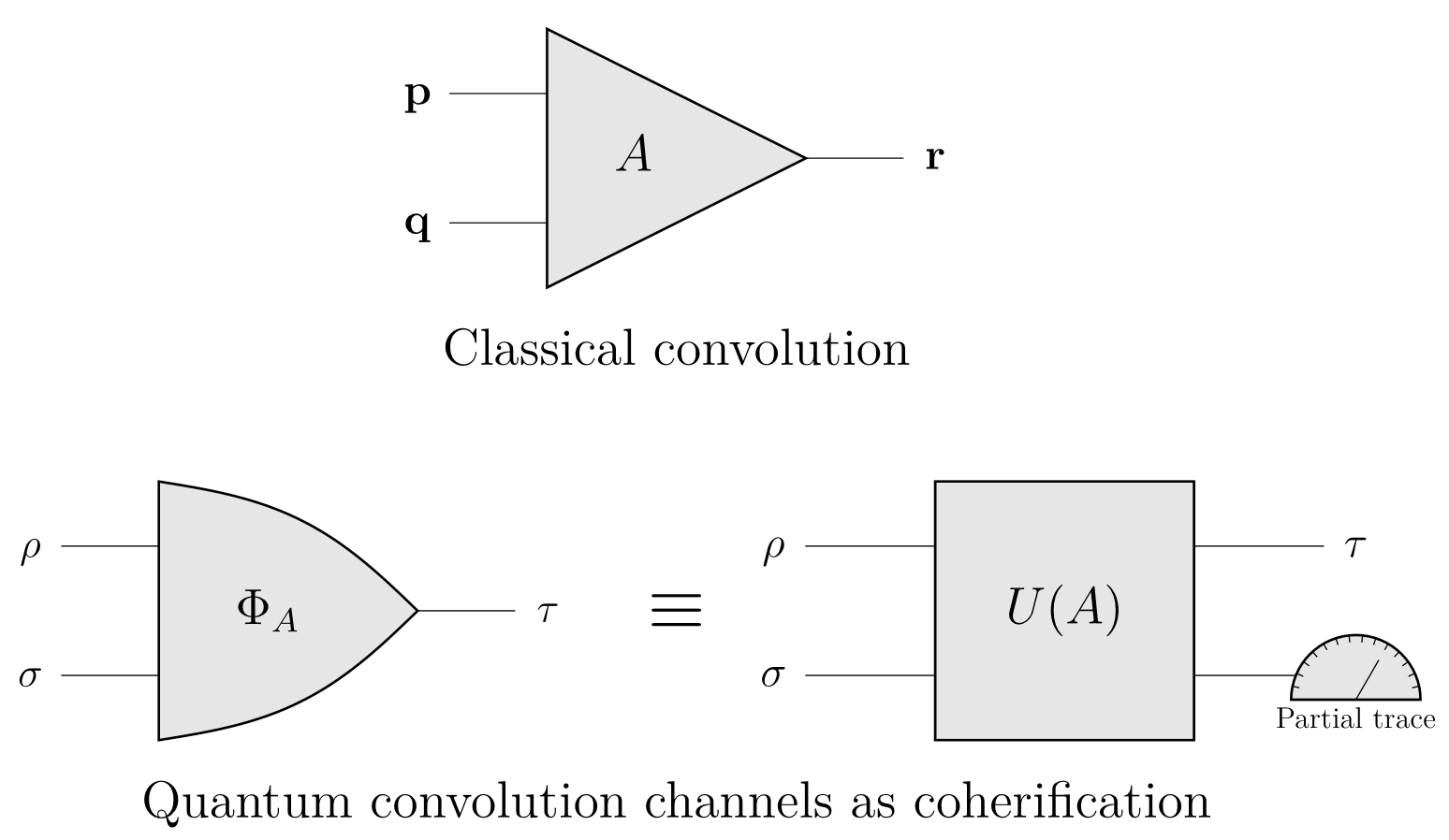
II Setting the scene
In the following subsections, we recall established notions and tools essential to understanding the results of our paper. We start with tristochastic tensors and a method for obtaining convolution channels by coherifying them. Then we proceed to entanglement properties of unitary operations and finish with orthogonal Latin squares and classical construction of 2-unitary gates based on pairs of such objects.
II.1 Tristochastic tensors and coherifications
Let us start by recalling the notions of stochasticity and tristochasticity in a classical framework which is a foundation for our work.
Definition 1.
A matrix is called stochastic if and . It is called bistochastic if and are both stochastic.
Definition 2.
A tensor is called tristochastic if and for any .
The class of tristochastic tensors, of special interest to us are permutation tensors, in which all entries are equal to either zero or one [28]. An example of a tristochastic permutation tensor for is provided below:
| (1) |
where the reader should imagine the square sub-matrices arranged in a cube.
The action of a tristochastic tensor on a pair of probability vectors , is defined analogically to the action of a stochastic matrix on the outer product , i.e. . In the case when each layer of is consecutive power of permutation matrix for permutation , as in the example (1), the action of simplifies to the ordinary convolution:
Thus the action of the tristochastic tensor might be interpreted as a generalization of the convolution of two probability vectors [28].
One can also define tristochasticity at the quantum level. To do so we first invoke a dynamical matrix of the channel via Choi-Jamiołkowski isomorphism [29, 30].
Definition 3.
Let be a quantum channel and a maximally entangled state. Then the dynamical matrix of the channel is defined as:
The transition from the dynamical matrix to the quantum channel is in turn defined by
| (2) |
The complete positivity and trace preserving properties (CPTP) of the channel are reflected by and , respectively.
In order to provide background, we start by invoking a definition of the unital channel, also known as a bistochastic channel, in a non-standard but equivalent way:
Definition 4.
A quantum channel defined by the dynamical matrix by
| (3) |
is bistochastic if the map:
| (4) |
also forms a valid quantum channel.
The above definition naturally generalizes to tristochastic channels.
Definition 5.
[28] Channel defined by dynamical matrix by
| (5) |
is called a tristochastic channel, if for any pair of density matrices the maps:
| (6) |
also forms a valid quantum channel.
An alternative, and much wider, approach to promote tristochasticity at the quantum level comes from the notion of coherification [31].
Definition 6.
[28] A coherification of a tristochastic tensor , is a channel , such that the diagonal of its dynamical matrix agrees with the elements of ,
| (7) |
with the CPTP properties of the channel guaranteed by the positivity and trace condition .
In other words, the coherification procedure is a search for preimages of the physical process of decoherence.
The recipe for coherification is ambiguous. Thus, following [28] from the entire set of coherifications of certain permutation tensor, we chose only those with maximal -norm coherification [31] defined by the sum of nondiagonal elements of modulus squared. It turns out that this choice is very fruitful because any such coherification of permutation tensor can be identified with a bipartite unitary matrix [28]:
| (8) |
where is the initial permutation tensor and are complex vectors satisfying , followed by a partial trace:
| (9) |
The dynamical matrix for such coherification of has a simple form
| (10) |
With unitary matrix as in equation (8). Therefore, from this point on, we will identify the coherification of a permutation tensor with corresponding unitary channel . Notice that in the proposed channel each basis can be freely adjusted in the learning process to a specific task, without losing general properties of coherification of permutation tensors. Thus one has a lot of free parameters handily combined in unitaries corresponding to the basis .
II.2 Entangling power of unitary operations
To characterize the properties of tristochastic channels discussed above, or equivalently unitary matrices (8), from the perspective of their ability to entangle and disentangle quantum systems, we recall the framework of entangling power of bipartite unitary gates and related notions.
Definition 7.
[1] Consider a unitary operation acting on a bipartite space with local dimension . The entangling power is defined as the average entanglement created by when acting on a pure product state ,
| (11) |
where the average is taken over Haar measure with respect to both subspaces.
In what follows we will use the linear entropy as the measure of entanglement, , with . The normalization in Definition 7 follows from the requirement
Theorem 1.
[32] A closed formula for entangling power reads
| (12) |
where the state is defined according to the Choi-Jamiołkowski isomorphism and is the swap operator.
A unitary operation is called 2-unitary, if the entangling power is maximal, or, equivalently, if partial transpose and reshuffled version are also unitary [2].
Further two quantities of interest are gate typicality (complementary to ) and disentangling power (defined as average entanglement left after the action of the gate on arbitrary maximally entangled state). They can both be given by the following formulas [27, 33]
| (13) | ||||
Note that entangling power and disentangling power are proportional [27], so the channels with maximal entangling power have also maximal disentangling power.
All the aforementioned properties of bipartite unitaries are invariant under local operations. For example, if for some unitary one has maximal entangling power, , then for any local rotations , . The work [17] presents a helpful tool to verify whether two unitaries and can be connected by such local operations.
Definition 8.
[17] Let be a 2-unitary, and be -element permutations. Then the invariant of the local rotations is given by:
| (14) |
where the sum over repeated indices is assumed.
Thus if two unitaries , and have different invariants, then one cannot be transformed into the other by local pre- and post-processing. Moreover, if all invariants for and have the same values, then they can be connected by local operations [17].
II.3 Orthogonal Latin squares
The last construction we refer to is a notion connected to combinatorics – Latin squares [34].
Definition 9.
A Latin square of dimension is a matrix with entries from the set such that in each row and each column contains all the elements of the set .
In other words, each column and each row contain all the numbers from to without repetitions, as can be seen in an exemplary Latin square of size 3 below,
| (15) |
To obtain a permutation tensor from the Latin square one may simply set . Examples of corresponding permutation (tri)stochastic tensor and Latin square are (1) and (15).
Together with the concept of Latin squares comes also the notion of their orthogonality.
Definition 10.
Two Latin squares, and , are said to be orthogonal if the set of pairs has distinct elements.
It is impossible to find two orthogonal Latin squares of dimension 2. However, for the exemplary Latin square (15) we can give an orthogonal Latin square
| (16) |
For any prime and prime-power dimension there exists a construction based on finite fields, yielding exactly pairwise-orthogonal Latin squares [35]. It is known that for any there exist at least two orthogonal Latin squares.
It has been shown in [27] that given two orthogonal Latin squares and in dimension one can directly construct a 2-unitary permutation matrix with in a straightforward way,
| (17) |
Such a construction is a nice example of coherification of permutation tensor , with basis vectors given by:
| (18) |
III Coherence measures for unitary operations
To distinguish the above construction from previously known ones in an operational framework we adapt the notion of coherence to describe unitary channels. In order to quantify a property akin to coherence for unitary operations we will consider average coherence generated by the action of a unitary matrix on the basis vectors, as given by -Rényi entropies applied to the amplitudes of the resulting states.
Let us take an arbitrary pure state . Its coherence with respect to the basis defined by a unitary matrix may be characterized as
| (19) |
where . For exponentials of these entropies,
| (20) | ||||
turn out to have simple interpretations related to the number of nonzero elements, linear entropy and maximal element – for details see Appendix A.
Using the above notion, we may define a measure of coherence of a unitary matrix as an average coherence of computational basis vectors:
| (21) |
Bipartite 2-unitary matrices offer an important degree of freedom to make use of, as two such matrices and are considered locally equivalent if there exist local unitaries , , , such that . Therefore each two-unitary corresponds to the entire range of values:
| (22) |
Let us consider two simple examples, starting with a case of local unitary operation, , evaluated with respect to the linear entropy. One easily finds that
| (23) |
The maximum is found by setting and keeping , while minimum is found when , where is the Fourier matrix of dimension ,
.
The same holds also if is an arbitrary permutation matrix and, in particular, a 2-unitary matrix constructed from two orthogonal Latin squares
| (24) |
which are values for a “bare” permutation () and Fourier matrices (, ), respectively. For a generic such range is not a priori trivial, in particular the maximal value points towards the non-vanishing coherence of the matrix, understood as ability of a given gate to generate nonzero coherences for any choice of local bases.
In some scenarios one may desire that in his circuit the average coherence of the output would lie in some particular range, independent of local pre- and post-processing of input basis states. Such a case corresponds exactly to a narrow coherence range.
For a more detailed discussion of this construction, further motivations and its properties, we encourage the readers to consult Appendix A.
IV Properties of tristochastic channels
In this section, we study the general properties of an entire class of coherifications of tristochastic tensors. As our main quantities of interest, we chose entangling power , disentangling power and gate typicality , because they allow us to determine the most important properties of tristochastic channels.
To get acquainted with the generalization of the following discussion into a framework of multi-stochastic channels we encourage the reader to study Appendix D.
Entangling power of a unitarity of size describes, how much the outcome is entangled on average for random input pure states and . Hence, after the partial trace, it gives us insight into how much the result of the channel becomes mixed.
Analogously disentangling power , proportional to the former [27], expresses how much the output of the "convolution channel" is pure, for maximally entangled input, which allows us to simultaneously reduce the system and minimize the loss of important information as in quantum convolutional neural networks [23].
Finally, the gate typicality describes the degree of subsystem exchange which, taking into account the partial trace, reveals which subsystem affects the output more.
Let us now consider underlying a coherification of a permutation tensor defined by a basis . By simple calculations, one obtains:
| (25) | ||||
This allows us establish bounds for entangling power and gate typicality for the unitary matrices of interest:
| (26) | ||||
Moreover, we obtained also the average values of entangling power and gate typicality over all tristochastic channels:
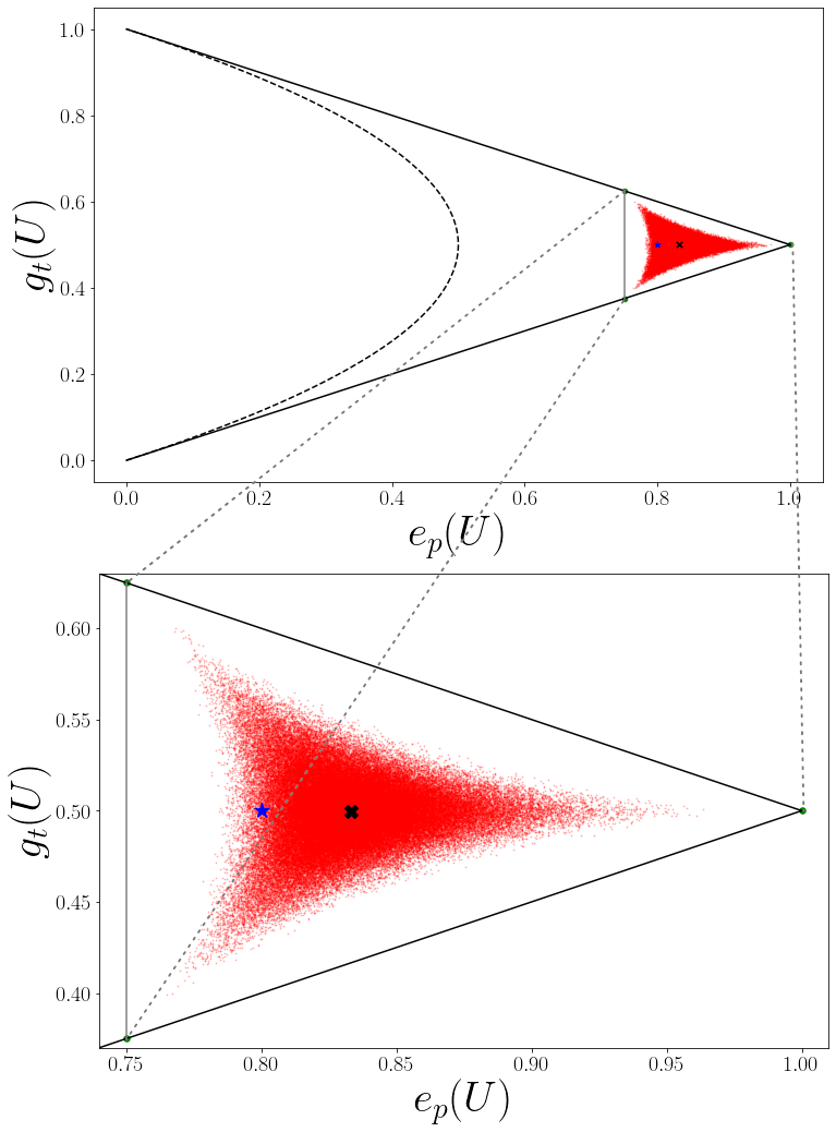
Note that the lower bound for entangling power for unitaries corresponding to coherifications of permutation tensors coincides with the upper bound of entangling power for block diagonal bipartite unitary matrices with blocks of size [4]. The exact derivation of those results is provided in Appendix B. The minimal values of entangling power are obtained for example when for any which corresponds to minimal gate typicality, or for , which corresponds to maximal gate typicality, see Fig. 2.
One can also consider the case when all the bases are mutually unbiased (MU) [36] i.e. for any two vectors from different basis and the overlap between basis vectors is given by
| (27) |
Taking to be a set of MU bases (MUBs), and defining, in turn, as the unitary representation of the coherification, resulting from (8) with such choice , the entangling power and gate typicality are given by:
which are exactly the average values of and .
The case of maximal entangling power is the most complex one. Before discussing it in detail let us reestablish the connection with (fully quantum) tristochasticity.
Theorem 2.
A unitary channel arising from coherification of a tristochastic permutation tensor attains the maximal entangling power if and only if it corresponds to a quantum tristochastic channel .
We present a proof of this theorem in Appendix B for the clarity of the text. To capture the connection between entangling power and (quantum) tristochasticity let us alter the notation (with no summation involved) to create the symmetry between indices . Then the condition for unitarity of gives
| (28) |
and the maximal entangling power imposes, from (64),
| (29) | ||||
| (30) |
On the other hand, one may interpret (29) or (30) as the conditions for unitarity of the following matrices
| (31) |
with maximal entangling power. This, composed with the partial trace, gives exactly the tristochastic channels in the "other directions" as in the Definition 5.
More intuitively, one can imagine a cube populated by states placed in positions corresponding to nonzero elements in such a way that each horizontal, vertical and “depth” slice contains an orthonormal basis on . This can be satisfied because there is only one non-zero state in each column, row and “depth-row”, since is a permutation tensor.
V Case study: 2-unitary from orthogonal Latin squares
Knowing the general properties of coherifications of permutation tensors, we may focus on the most important case of channels with maximal entangling and disentangling power. Our main construction of such channels can be seen as a generalization of permutations with maximal entangling power from [2] which we take as a starting point for our discussion. Let be a tristochastic permutation tensor of interest, a corresponding Latin square and Latin square orthogonal to , then the maximally disentangling unitary matrix in the channel (8) can be constructed as
| (32) |
with the same relation between Latin squares and the permutation tensor with vectors is in (18).
Unitary matrix (17) has maximal entangling power and gate typicality . Since orthogonal Latin squares exist in any dimension except and [37], construction (17) is rather general. On the downside, it does not provide any free parameters except possible phases.
Regardless of the abovementioned limitation, channels defined via (17) can be very useful in controlled disentangling of quantum states, which is the key property of qCNN building blocks [23, 24, 25, 26]. As the case study, which can be efficiently implemented in the modern quantum computer, we consider a channel constructed via (17) for two ququarts. Since each ququart can be interpreted as a pair of qubits, from the perspective of quantum hardware the channel is a unitary acting on four qubits, followed by a partial trace on two of those.
In general, there is a large freedom in the construction of orthogonal Latin squares and , which correspond to local gates. One may simultaneously permute rows and columns of these squares, which corresponds to local preprocessing of the unitary channel (17) or permute the symbols in the Latin squares, which corresponds to local postprocessing of , resulting in a locally equivalent channel of the form . To reduce the number of such "repetitive" channels, we fixed the first columns of and and the first row of to be , which almost completely erases such degeneration. After all the eliminations associated with local preprocessing and postprocessing, the remaining pair of orthogonal Latin squares in dimension is given below
This pair gives a unitary channel which can be viewed either as two ququart maximally (dis)entangling gate or, after decomposing the ququarts, a four qubit highly (dis)entangling gate. It can be implemented using a circuit of depth 11 using 18 nearest-neighbour gates in the following way:
| (33) |
Notice that one left outer layer and two right outer layers can be "pulled out" as local ququart pre- and postprocessing reducing the circuit to gates organized in 8 layers. The matrix acts on two ququarts each represented by a pair of qubits encompassed by a dashed rectangle. Up to our knowledge, this is the most efficient way to implement a 2-unitary matrix using only nearest neighbour gates in linear architecture.
For the sake of completeness, we recall that is a permutation matrix of order , thus all the vectors from the computational basis are mapped onto each other, so the results are separable.
On the other hand, it is interesting that there exists a basis of maximally entangled states of two ququarts, for which all vectors are mapped by onto separable states. Therefore the action of on all the vectors from this basis gives a set of pure states, which overlap with the ququart basis.
To present this basis and discuss more of its profitable properties let us first introduce a suitable notation. Let
denote the Bell states, entangling the first or second qubits from each ququart. Then the discussed basis takes the form
| (34) |
The vectors from consecutive rows of basis (34) map under onto basis vectors
on the first ququart and the vectors from consecutive columns map onto basis vectors
on the second ququart. Thus the choice of type of Bell states ( or ) determines the result on the first ququart, and the signs chosen in them (eg. or ) determine the result on the second ququart.
Due to such an elegant mapping of basis vectors (34) under we can say even more about the action of on maximally entangled states of two ququarts. For example, if one constructs such a state as a superposition of vectors from one row (or column) from basis (34), then after the action of all these basis vectors will map on the same pure state on the first (second) ququart. Therefore the action of on such superposition also gives a separable state, hence action of gives pure output.
Generalizing this property on the pairs or triples of columns and row form (34) one obtains the following result.
Theorem 3.
The generalization of the above discussion for multipartite channels is presented in Appendix D.4.
As mentioned at the beginning of this section, may be used as a building block in quantum convolutional neural networks (qCNN). One can create qCNN acting on several ququarts, by stacking the discussed channel parallelly or sequentially, with possible single-ququart channels along the way. To find a basis of entangled states transformed by such circuits into pure computational states, one only needs to iteratively combine the basis (34) with itself in an appropriate way.
VI New classes of genuinely quantum 2 unitary gates
In this section, we introduce new continuous families of 2-unitary gates emerging from coherifications of permutation tensors.
First, let us rewrite the equations (28–30) as a conditions of unitarity for matrices, defined by
| (35) | ||||
where in each sum there is in fact only one nonzero vector due to being a permutation tensor.
Thanks to the structure above we may leverage an algorithm akin to the Sinkhorn approach used in [15]. Cycling through the sets , we orthonormalize each element of the set using polar decomposition. The standard complexity of polar decomposition of a matrix of size , using SVD, behaves as . When full matrix is considered as in [15] (), this results in complexity . The proposed approach relies on the decomposition of square matrices , of size each, resulting in complexity .
Furthermore, our approach limits the dimensionality of the space explored and as such, should be faster to converge than the methods employed in the full space 111Assuming that a solution exists within the limited space, which is not guaranteed.. Finally, let us point out that the number of complex parameters, thanks to the choice of the tristochastic tensor and local freedom to fix , is equal to , whereas the previous approaches have, in general, parameters, again highlighting reduction of complexity.
The dimension was already discussed in [28]. For the peculiar dimension , despite extensive numerical searches, we did not find a coherification of any permutation tensor with entangling power larger than [39]. In Appendix C we present an exemplary orthogonal matrix which can be constructed as a coherification of a tristochastic tensor, achieves this bound and could serve as a candidate for the most entangling orthogonal gate of order . One might think, that the construction (17) encompasses all the coherifications of permutation tensors since it is the case for , which can be verified by direct (exhaustive) calculations. Nevertheless, in dimension it is possible to find nontrivial sets of bases which generate unitary channels with maximal entangling power, .
In particular, by focusing our attention on cyclic permutation tensors and their coherifications constructed using bases with cyclic amplitude structures,
| (36) |
where denotes the addition modulo , together with fixing the first basis as the computational basis, , we were able to derive two novel continuous families of 2-unitary matrices of dimension . In the following subsections we will discuss a 2-parameter family for dimension and a family for dimension characterized by two bases with cyclic structure. The aforementioned new classes of -unitary matrices, which will be presented in the following subsections, are genuinely quantum [15], in the sense, that they are not locally equivalent to any permutation tensor from equation (17):
for any local pre- and postprocessing.
Both of the presented classes in dimensions and , similarly as permutations, can be further extended by the multiplication by a diagonal unitary matrix with arbitrary phases, giving additional and nonlocal parameters, respectively.
VI.1 Dimension 7
The 2-parameter family of 2-unitary operations of order found for is characterized by seven bases , which are summarized in Fig. 4. After fixing the first basis as equal to the computational basis using local rotation, the remaining six bases are particularly elegant and can be characterized by just two non-zero amplitudes: and , nine distinct constant phases from the set , and two free phases , as summarised in Fig. 4.
In order to compare this family to the already known solutions based on Latin squares we have resorted to the 4-th order invariant defined in (14) with the permutations
in line with the invariant used in [17] for the case of 36 officers. The final expression is given by
| (37) | ||||
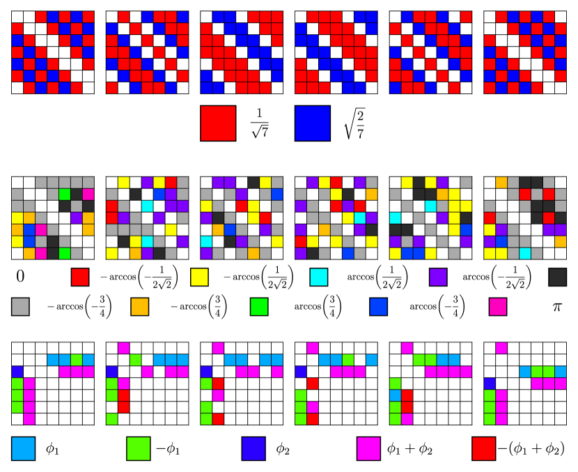
Global minima and maxima of this function can be easily found, thus bounding it by
| (38) |
with the lower bound being well above the same invariant calculated for any 2-unitary permutation in dimension , equal to . This is enough to demonstrate that the entire family is locally inequivalent to any 2-unitary permutation .
In order to bound the coherence from the inside we calculated as approximation of upper limit and with the Fourier as the lower limit of the approximation. Interestingly, for all we find . After maximizing over the parameters we find that for all
| (39) |
Surprisingly, attempts to improve these bounds using simulated annealing techniques do not show any improvement over the simple approach we have used. The table of estimated coherence ranges obtained for other entropies and comparison with permutations is presented in Appendix A.
The obtained solution provides also an explicit recipe to generate states of four systems of dimension by
VI.2 Dimension 9
In case of dimension let us consider unitary matrices of size composed from consequent basis vectors ,
| (40) |
Let us define a cyclic permutation on blocks,
| (41) |
which we use in defining
| (42) |
where is the matrix representation of permutation . As before, we may fix the first basis to be given by the computational basis,
| (43) |
The remaining two bases and are parameterized by two independent cyclic unitary matrices ,
| (44) |
with and and such that .
Then, we define for
| (45) |
with permutations
| (46) |
and
| (47) |
which, overall, yields the structure of entries as in Fig. 5, where each distinct number is marked by a different colour. The 2-unitary matrix can be reconstructed using (8) as:
| (48) |
with as described in equation (45) and . Note that the entire matrix has 4 free parameters, since unitarity conditions for (and ) reduce the number of their free parameters to (and ), which in turn guarantees 2-unitarity conditions on constructed from the bases according to the recipe (8).
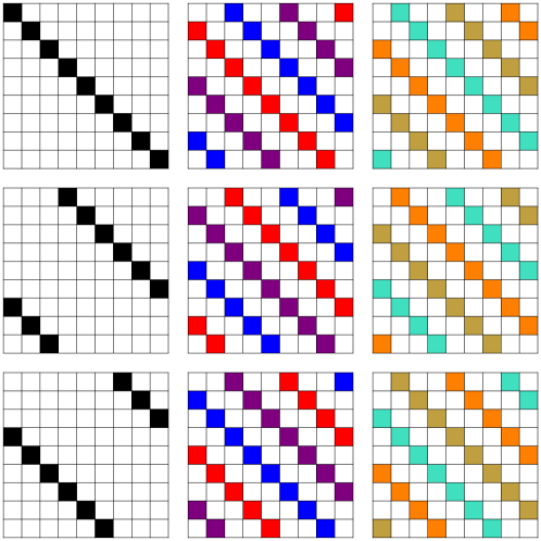
Notice, that for limit values of parameters the matrix degenerates to a permutation matrices. Thus it can be interpreted as a generalization and extension of 2-unitary permutations into continuous families of 2-unitary matrices.
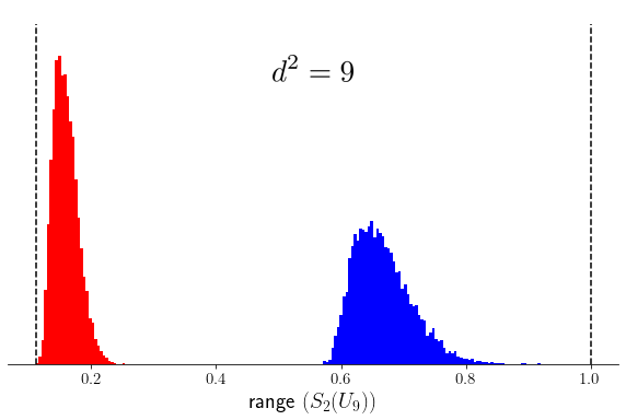
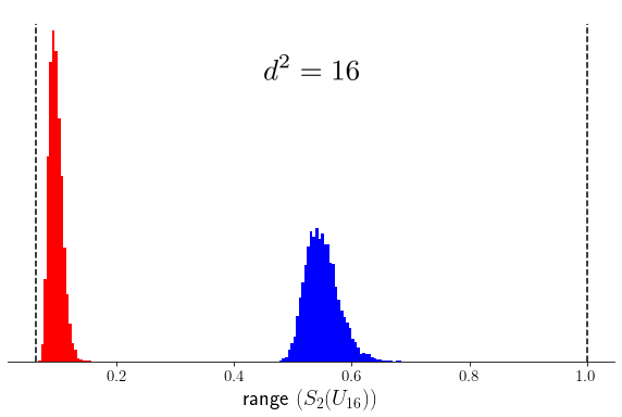
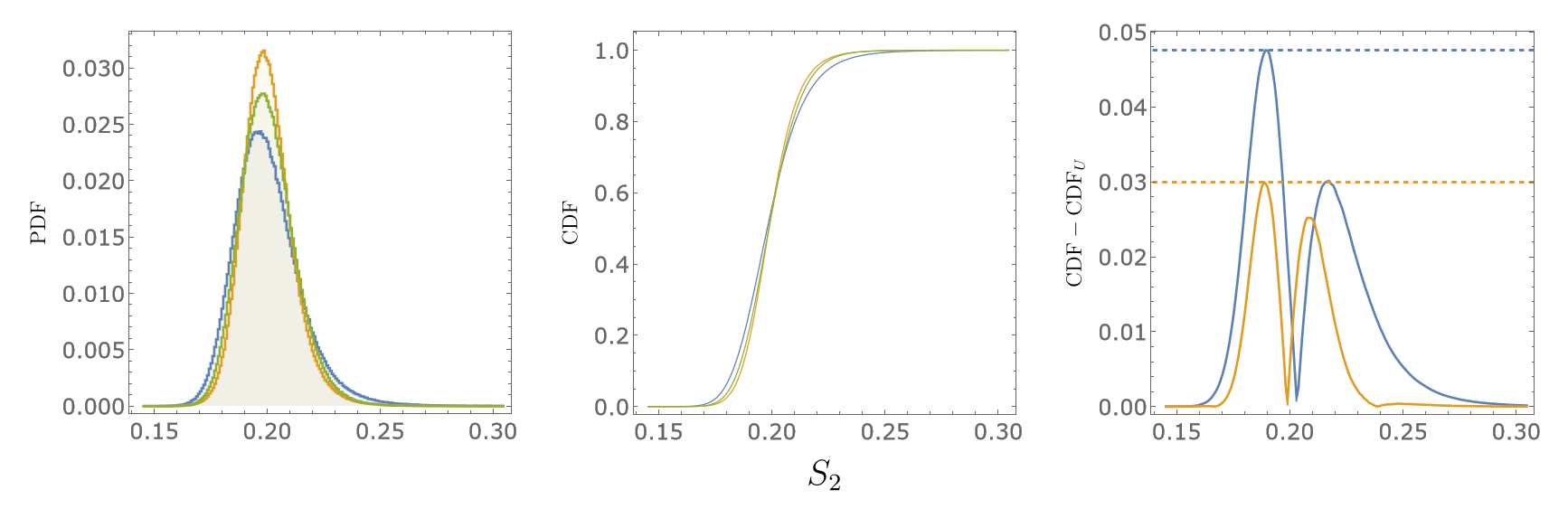
Using the invariants we have not been able to demonstrate local inequivalence of from the 2-unitary permutations, and thus we resorted to a statistical approach used in [14]. Histograms of generated entanglement (see Fig. 6) show that the family is indeed locally distinct from permutations. We verify this quantitatively by using the two-sample Kolmogorov-Smirnov test with samples per distribution, which yields the confidence level of at most , implying that the sample obtained from is different from the standard construction for the 2-unitary permutations with probability .
We evaluate the coherence measures and to find an inner bound on the coherence range of any member of the family as
| (49) | ||||
The table of estimated coherence ranges obtained for other entropies and comparison with permutations is presented in Appendix A
The obtained solution provides a recipe to generate the absolutely maximally entangled state by the same token as in the dimension .
VII Outlook and conclusions
Our work serves as a first step into the subject of generation and application of continuous parametrizable families of 2-unitary matrices (perfect tensors) and "quantum convolutions". Thanks to the adjustable free parameters, our findings may serve as a prototype for trainable building blocks in quantum convolutional neural networks.
First we considered the entire set of coherifications of permutation tensors, to show the full range of possibilities for such a framework. Next, we focused on the known examples of two-unitary matrices constructed from orthogonal Latin squares to present its limited, nevertheless quite remarkable, capabilities in disentangling not only quantum states but the entire maximally entangled basis. Finally, using the framework of coherification of permutation tensors, we introduced new continuous families of 2-unitary matrices in dimensions and , together with the discussion of their properties. We also presented arguments for their non-equivalence with previous constructions and that their parametrizations cannot be considered as local ones. Moreover, using a new measure of coherence for unitary operations, derived from the range of Rényi entropies that can be created from computational basis’ input, we highlighted the ability to generate nontrivial coherences for any local pre- and post-processing – a crucial property for the future quantum convolutional networks.
Thus we placed the first steps towards such development of the theory of 2-unitary channels, which will allow for their parametric optimization for specific tasks. It is crucial to stress at this point that the introduced families are exemplary and the introduced framework is not limited to them. We emphasise that 2-unitary matrices based on the construction introduced in this work are not equivalent to either the standard orthogonal Latin squares construction or other non-standard approaches. We demonstrated the former explicitly, using invariants and statistical methods [15, 16]. The latter can be found by noticing either a mismatch between the block structure [15] of the solutions or the lack of continuous non-local parameterization [17].
The coherification of permutation tensors was primarily applied to tristochastic tensors resulting in bipartite unitary matrices. However, it can be also generalized for multistochastic permutation tensors giving multipartite unitaries with large entangling and disentangling capacities, see Appendix D.
Our work prompts important and intriguing questions worth further investigation. First and foremost, it is tempting to try to generalize our findings into a universal recipe for continuous families of multi-unitary matrices in arbitrary dimension . The dimensions are of special interest due to possible applicability in quantum circuits. The next open problem is the reasonable construction of a quantum circuit that corresponds to such channels, which is crucial for real-life applications. Finally, the issue of connecting the convolution channels into larger networks has only been touched upon and requires further study for more general channels.
Acknowledgments
It is a pleasure to thank Wojciech Bruzda and Adam Burchardt for fruitful discussions. Moreover, we thank Grzegorz Rajchel-Mieldzioć, Arul Lakshminarayan, Suhail Rather and Michael Zwolak for valuable suggestions. Financial support by NCN under the Quantera project no. 2021/03/Y/ST2/00193 and PRELUDIUM BIS no. DEC-2019/35/O/ST2/01049 is gratefully acknowledged.
Appendix A Measure of coherence of a unitary operation
It is easy to measure the coherence of any pure state with respect to any given basis by considering the entropic properties of the resulting probability distribution. Let us take a state . Its coherence with respect to the basis defined by a unitary matrix is given by (19). For exponentials of these entropies, presented in equation (20), turn out to have simple interpretations. In particular, counts the nonzero elements of and is equal only to the absolute value of the largest element of . Finally, is closely connected to the linear entropy, often used in the context of entanglement.
Based on the above, we may define measures for coherence of a unitary matrix based on average (or total) coherence generated on the computational basis,
| (50) | |||
| (51) |
where, again, the simple interpretation of and , is the average number of elements per vector and average maximal element. In this case, we have two apparent degrees of freedom to introduce – freedom to change the measurement basis to , and to rotate the operation to . This yields the following expressions
| (52) | |||
| (53) |
One can easily see that we may write explicitly
| (54) | ||||
| (55) |
with . The quantity takes a particularly elegant form, reminiscent of the Welch bounds [40]. Using these bounds we find for
| (56) |
However, this bound is far from saturable, as for one would need at least vectors.
Such measures would be rendered meaningless given full freedom of basis choice – every unitary can be equivalent to a diagonal matrix, or a Fourier matrix by a proper choice of alone, thus reaching minimal and maximal values, respectively. However, in realistic settings, we will usually be dealing with partial freedom.
For instance, it is natural to assume that we deal with a bipartite system, , and to restrict our attention to local bases, . Then one may consider the possible range of entropies achievable,
| (57) |
corresponding directly to formula (22) by relation .
Equipped with these, we may start asking questions about possible ranges for different operators. One certain thing one can say is that if , then we cover the entire possible range for a given entropic measure, for example
| (58) |
which are values for permutation and Hadamard matrices, respectively. The same holds also if is a permutation matrix, in particular, constructed from two orthogonal Latin squares
| (59) |
which are values for a permutation () and Hadamard matrices (, ), respectively. For a generic such range is not a priori trivial, especially the minimal value points towards the non-vanishing coherence of the matrix.
For instance our solution id dimension with yields
The general form of the minimum is given by
In the table below we present estimated coherence ranges for and and compare them to permutations.
| 0 | 2 | |||||
| min | max | min | max | min | max | |
| 1 | 49 | 1 | 1 | |||
| 49 | 0.042 | 0.27… | ||||
| 1 | 81 | 1 | 1 | |||
| 81 | ||||||
Appendix B Calculation of entangling power for tristochastic channels
In this Appendix, we explicitly derive the results discussed in Section IV.
First, let us focus on the entangling power and gate typicality for the coherification of the general permutation tensor, . Taking into account that is a permutation tensor and is a basis vector from the basis, one can calculate that:
| (60) | ||||
Therefore we immediately get the following bounds
Using the above, we establish a general bound for the entangling power and gate typicality for the coherifications of permutation tensors
| (61) |
However, after a closer look, one can obtain a tighter bound for entangling power. Let us consider the sum ,
| (62) | ||||
In order to understand this expression better we need to manipulate the indices to our advantage. In the first and second sums, we see that for each value of and there exists only one value of such that is nonzero, hence only these components contribute to the sums. Moreover, in the first sum both and are simultaneously nonzero only if , because is a permutation tensor. By the similar argument let us define as the only value of such that the product is nonzero. After all this renaming above calculations can be summarized as
where in the last line we used the fact that is a sum of squared amplitudes of two coefficients of vector in the basis , so by normalization it must be smaller than . Inserting obtained bound for into the formula for entangling power one finds:
| (63) |
If all the bases are mutually unbiased [36], then for and as in equation (27), we obtain a unitary with unbiased basis in (8). This, in turn, lets us explicitly calculate:
No matter which permutation tensor we consider.
Next, let’s discuss the average values of entangling power and gate typicality .
Theorem 4.
The average value of entangling power and gate typicality of channels corresponding to coherifications of any permutation tensor is the same as for , presented above.
Proof.
Let us start by rewriting each basis as a unitary matrix ,
Hence average over all bases can be rephrased as the integration of entangling power and gate typicality over with Haar measures. Moreover, both entangling power and gate typicality are linear combinations of expressions of the form , so one might change the order of integration and summation and focus only on the following integral:
for , where we used the fact that and unitary invariants of Haar measure. For one gets
Since the average value of over all possible bases is the same as for MUB’s, the average value of entangling power and gate typicality is the same as for ’s. ∎
After becoming acquainted with the behaviour of coherifications of permutation tensor we are ready to present the proof of the Theorem 2.
Proof.
Assume that there exists some coherification with maximal entangling power . Since maximal entangling power translates to the maximal value of the sum , by equation (62) (and discussion therein), it corresponds to
| (64) |
| (65) |
On the other hand, quantum tristochasticity of the channel is equivalent to the condition that,
for any , where is a maximally mixed state placed on any entry [28].
This property, in turn, is equivalent to conditions (64),(65). Which can be seen from examination of the off-diagonal values of :
| (66) |
which is true for any if and only if all terms in (64) are equal to zero. This, in turn, is equivalent to their sum being equal to zero due to their nonnegativity.
By placing the maximally mixed state in the second argument one gets
| (67) | ||||
where is such that . Which, by the same token as above, is equivalent to the condition (65).
∎
Appendix C Orthogonal gates with large entangling power in dimension
Although we did not find quhex bipartite unitary channels with , we found several solutions attaining the same value of entangling power as the record for orthogonal channels: [39], Below we present the corresponding Latin square and a bases giving such an examplary channel by equation (8). The Latin square reads:
and the corresponding bases, given as orthogonal matrices, are
where , , , , .
In contrast to the previous results of orthogonal matrices close to -unitary, obtained in [39] by a numerical search, we propose a heuristic construction which leads to the explicit analytic result which can be extended into a continuous family of unitary matrices with the same entangling power close to unity.
Appendix D Quantum Multistochastic Channels
In this section, we generalize our results for the coherifications of multi-stochastic permutation tensors. To do so, we must start by generalizing the notion of tristochasticity into multistochasticity. On the classical level, such an abstraction is quite natural.
Definition 11.
A tensor is called multistochastic if and for .
The generalization on the quantum level is performed in the same spirit but gives a slightly more complicated result
Definition 12.
[28] Channel defined by dynamical matrix by
| (68) |
is called an -stochastic channel, if for any sequence of density matrices and any index the map:
| (69) |
also forms a valid quantum channel.
In constructions of multi-stochastic channels, we also refer to the generalizations of Latin squares - Latin cubes and Latin hypercubes
Definition 13.
A Latin hypercube of dimension is a tensor with entries from the set , such that every hypercolumn contains all the elements from the set .
Note that the secondary indices run from to – a choice which will prove itself convenient soon.
We observe that by fixing all the indices in a Latin hypercube except two one obtains a Latin square. We will call any such square a Latin subsquare. Using this observation we define orthogonal Latin hypercubes as in [34].
Definition 14.
Two Latin hypercubes are orthogonal if each corresponding pair of Latin subsquares are orthogonal.
At this point, one may wonder why we choose such a peculiar way to enumerate the indices of Latin hypercubes. We do so for the sake of natural translation between Latin hypercubes (and squares) and permutation tensors and vice versa. Notice that
| (70) |
satisfy all the necessary conditions of the permutation tensor, because the sum over any of the indices on the right-hand side of (70) gives one. On the other hand, one may define the Latin hypercube by
| (71) |
And once again the defining property of Latin hypercubes is satisfied, because for any fixed values of and two different , if
then
so sum over index of does not give one.
D.1 Entangling power in multipartite systems
Entanglement becomes significantly more complex when shifting from bipartite to multipartite systems – there is no unique entanglement measure, and to make matters worse, it requires more than a single one for full description. Thus, multipartite entanglement becomes more of a landscape and less of a line [41, 42, 43]. It follows naturally, that entangling power can also be defined in many ways. In our analysis we focus on the definition provided by [44].
Definition 15.
The entangling power for an partite unitary channel is defined as the entanglement generated by the map averaged over all possible separable states ,
| (72) |
where the measure of multipartite entanglement is taken to be the average of entanglements with respect to all possible bipartitions of the system.
| (73) |
There exists a general analytical formula for multipartite entangling power, which we present below in the simplified form with dimensions of all components equal .
Theorem 5.
[44] The entangling power for an partite unitary channel can be calculated as an average of entangling powers with respect to all bipartitions ,
| (74) |
Entangling power of with respect to bipartition in turn, is given by
| (75) |
Where the sum is also taken with respect to all the bipartitions of subsystems.
D.2 Coherification of multi–stochastic permutation tensors
Now we are equipped with all the necessary tools to study coherifications of -stochastic permutation tensors . As it turns out, those coherifications can also be realized as a unitary
| (76) |
where for any the vectors forms a dimensional basis; followed by a partial trace on all subsystems except the first one. For more detailed derivations and examples see Appendix E.
The dynamical matrix of the channel thus also has a form similar to (10)
If one defines
| (77) |
the condition of unitarity of (76) can be expressed in the spirit of formulas (28) as
| (78) |
and the complementary conditions read,
| (79) | ||||
These conditions let us define unitary channels in all the "other directions" analogous as in (31), hence they correspond to (quantum) -stochasticity of .
One may expect that conditions (78),(79) would be sufficient to guarantee also maximal entangling power of the multipartite unitary channel , similarly as in the case of tristochastic permutation tensors. However, this is not the case. In the formula of multipartite entangling power (74), one must consider all the bipartitions for both input and output indices of : and , see (75). On the other hand, in the equations (78), (79) all except one output indices of : are always together.
D.3 Latin (hyper)cubes and their connection to maximal
Finally, we present a coherification of -stochastic permutation tensor, which is both (quantum) multi-stochastic and has a maximal multipartite entangling power.
Let be a permutation tensor, which coherification we will construct, corresponding Latin hypercube and be Latin hypercubes such that all Latin hypercubes are mutually orthogonal. Then the multipartite unitary stemming from the coherifiaction has a form
| (80) |
Because the Latin hypercubes are mutually orthogonal, by Theorem 5.12 from [34], construction (80) gives a large permutation tensor, hence a unitary matrix.
To argue the maximum entangling power of (80) we use the fact that is an AME state (see [3] section 3.2) hence all the partitions onto and in (75) gives maximal possible contribution to entangling power. From the fact that is an AME state also follows a simple argument for the multi-stochasticity of (from (80)). The maximal entanglement of with respect to bipartition , guarantee that the matrix:
| (81) |
is unitary for any . In Appendix F, Theorem 6 we present also an alternative the proof of multi stochasticity for corresponding to unitary channel (80).
Although the existence of orthogonal Latin hypercubes is explored less than for orthogonal Latin squares, some results are known. For example, thanks to Theorem 5.4 form [34], we are guaranteed that for being prime power and there exist at least mutually orthogonal Latin hypercubes of order . This means that in the prime power dimension our construction is valid if .
D.4 Case study: 3-unitary from orthogonal Latin cubes
To present the usefulness of the multi-stochastic quantum channel, we briefly discuss the channel obtained from (80) using three orthogonal Latin cubes of dimension presented in figure 7.
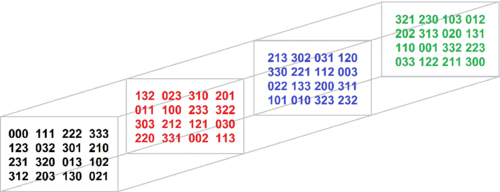
Unitary (80) from this channel acts on three quqarts, which we interpret as three pairs of qubits, same as in Section V. In this case, there also exists a maximally entangled basis, all of which elements are mapped into fully separable states of three ququarts. Therefore the action of on those basis vectors gives pure states overlapping with the basis on quart.
To present this basis let us entangle the first qubits from all ququarts and the second qubits from all quqarts by states :
| (82) | ||||
Then the abovementioned basis has a form , where the indices and both sights are independent. Moreover, after appropriate multiplication by of the basis vectors , one could repeat the discussion from Section V, together with the analogue of Theorem 3, but this time on the three ququarts.
Appendix E Coherification of multi stochastic permutation tensors
In this Appendix, we generalize the construction of optimal coherifications from [28] for multi-stochastic permutation tensor. Following ref. [28] a coherification is considered to be ’optimal’ if the norm-2 coherence achieves its maximal value. This measure quantifies the average contribution of the non-diagonal entries of the dynamical matrix ,
| (83) |
Here is a given coherification of a tristochastic tensor , are eigenvalues of dynamical matrix and are eigenvalues of the dynamical matrix of diagonal coherification without any non-diagonal terms.
Let us consider the Kraus representation of the channel . The Kraus operators are, in this case rectangular matrices such that
so the connection between Kraus operators and the Dynamical matrix is given as
where denotes the combination of indices in the following way: while the multi index is constructed as .
To ensure that is a coherification of , we therefore demand that . This implies that any Kraus operator can have nonzero entry if and only if is nonzero. Because for each there exist only one such that we may enumerate those entries as . Thus we will slightly abuse our notation, and use a multi-index to denote . For example for the -stochastic permutation tensor (4-dimensional hypercube):
| (84) |
we get Kraus operators of the form:
| (85) |
Next we examine the condition . Because in each column of each Kraus operator, there is only one nonzero parameter from the diagonal terms of we obtain the condition .
Moreover because in row of each all coefficient have first index the same and equal to (by the construction of these coefficients), from the non-diagonal terms of we get . Thus for each value of the vectors forms an orthonormal set, therefore the norm two coherification of would be maximal if this orthonormal set would spam the same space for any value of . Hence the number of Kraus operators, which is equal to the dimension of vector space in which lives, must be equal . The norm two coherence of that coherification reads:
| (86) | ||||
where the third step comes from the decomposition of each (normalized) vector in the basis .
For such coherification of -stochastic permutation tensor the construction of a quantum channel via a unitary channel and partial trace is analogical as in [28]. Because we have Kraus operators we might construct unitary from them in the following way
| (87) | ||||
where we exchanged the index , enumerating Kaus operators, by the set of indices .
Moreover, such unitaries once again have a structure of block diagonal unitary matrices with blocks: , multiplied by some permutation matrix corresponding to underlying permutation tensor :
For example, for the permutation tensor (84) we get:
| (88) |
for which the block diagonal matrix yields:
| (89) |
where we enumerated the parameters once again by .
Thus the coherification of permutation tensor may be considered as a unitary matrix between subsystems with dimension , followed by partial trace over all subsystems except one.
Appendix F Multistochasticity of unitary constructed form orthogonal Latin hypercubes
In this Appendix, we present a proof of (quantum) multi-stochasticity of unitary operations constructed from orthogonal Latin cubes given in (80). However, before doing so, we must gently rewrite unitary matrix of interes.
Lemma 1.
Any unitary channel of the form (80):
| (90) |
can be expressed by a new set on orthogonal Latin hypercubes as:
| (91) |
Proof.
By Theorem 5.3 from [34] the problem of constructing orthogonal Latin hypercubes is equivalent to the construction of maximal distance separable (MDS) code of words of length from an alphabet of length , and distance between words equal [34]. Let us present this code as rows in orthogonal array :
where the distance between any two rows, equal , is understood as a number of coordinates in which two rows differ.
Notice that the distances between rows in do not change if one moves the last columns to the front and put the rows in order to construct a new array :
where we renamed the indices:
Thus we obtain a new maximal distance separable code which guarantees that the corresponding hypercubes are in fact orthogonal Latin hypercubes. ∎
Theorem 6.
The unitary channels defined by (80) is a (quantum) -stochastic channel.
Proof.
By the above lemma, we may write the unitary matrix(80) in a form (91), so the channel acting on the set of input states, of which is totally mixed gives:
| (92) | ||||
In the last step, we used the fact that each density matrix has the same values of upper and lower indices, and the sums run over all values of indices. ∎
References
- Zanardi et al. [2000] P. Zanardi, C. Zalka, and L. Faoro, Entangling power of quantum evolutions, Phys. Rev. A 62, 030301 (2000).
- Clarisse et al. [2005] L. Clarisse, S. Ghosh, S. Severini, and A. Sudbery, Entangling power of permutations, Phys. Rev. A 72, 012314 (2005).
- Rico [2020] A. A. Rico, Absolutely maximally entangled states in small system sizes, Master Thesis, University of Innsbruck (2020).
- Aravinda et al. [2021] S. Aravinda, S. A. Rather, and A. Lakshminarayan, From dual-unitary to quantum Bernoulli circuits: Role of the entangling power in constructing a quantum ergodic hierarchy, Phys. Rev. Res. 3, 043034 (2021).
- Reed and Solomon [1960] I. S. Reed and G. Solomon, Polynomial codes over certain finite fields, Journal of the Society for Industrial and Applied Mathematics 8, 300 (1960).
- Scott [2004] A. J. Scott, Multipartite entanglement, quantum-error-correcting codes, and entangling power of quantum evolutions, Phys. Rev. A 69, 052330 (2004).
- Latorre and Sierra [2015] J. I. Latorre and G. Sierra, Holographic codes, arXiv preprint arXiv: 1502.06618 (2015).
- Pastawski et al. [2015] F. Pastawski, B. Yoshida, D. Harlow, and J. Preskill, Holographic quantum error-correcting codes: Toy models for the bulk/boundary correspondence, J. High Energy Phys. 6, 1029 (2015).
- Helwig et al. [2012] W. Helwig, W. Cui, J. I. Latorre, A. Riera, and H.-K. Lo, Absolute maximal entanglement and quantum secret sharing, Phys. Rev. A 86, 052335 (2012).
- Bertini et al. [2019] B. Bertini, P. Kos, and T. Prosen, Exact correlation functions for dual-unitary lattice models in dimensions, Phys. Rev. Lett. 123, 210601 (2019).
- Harper [2022] J. Harper, Perfect tensor hyperthreads, J. High Energy Phys. 2022, 239 (2022).
- Goyeneche et al. [2015] D. Goyeneche, D. Alsina, J. I. Latorre, A. Riera, and K. Życzkowski, Absolutely maximally entangled states, combinatorial designs, and multiunitary matrices, Phys. Rev. A 92, 032316 (2015).
- Raissi et al. [2022] Z. Raissi, A. Burchardt, and E. Barnes, General stabilizer approach for constructing highly entangled graph states, Phys. Rev. A 106, 062424 (2022).
- Rather et al. [2022a] S. A. Rather, S. Aravinda, and A. Lakshminarayan, Construction and local equivalence of dual-unitary operators: From dynamical maps to quantum combinatorial designs, PRX Quantum 3, 040331 (2022a).
- Rather et al. [2022b] S. A. Rather, A. Burchardt, W. Bruzda, G. Rajchel-Mieldzioć, A. Lakshminarayan, and K. Życzkowski, Thirty-six entangled officers of Euler: Quantum solution to a classically impossible problem, Phys. Rev. Lett. 128, 080507 (2022b).
- Rather [2023] S. A. Rather, Construction of perfect tensors using biunimodular vectors, arXiv preprint arXiv: 2309.01504 (2023).
- Rather et al. [2023] S. A. Rather, N. Ramadas, V. Kodiyalam, and A. Lakshminarayan, Absolutely maximally entangled state equivalence and the construction of infinite quantum solutions to the problem of 36 officers of Euler, Phys. Rev. A 108 (2023).
- Fukushima [1988] K. Fukushima, Neocognitron: A hierarchical neural network capable of visual pattern recognition, Neural Networks 1, 119 (1988).
- Schmidhuber [2015] J. Schmidhuber, Deep learning in neural networks: An overview, Neural Networks 61, 85 (2015).
- Baldi and Chauvin [1993] P. Baldi and Y. Chauvin, Neural networks for fingerprint recognition, Neural Computation 5, 402–418 (1993).
- Muller et al. [2005] U. Muller, J. Ben, E. Cosatto, B. Flepp, and Y. Cun, Off-road obstacle avoidance through end-to-end learning, in Advances in Neural Information Processing Systems, Vol. 18, edited by Y. Weiss, B. Schölkopf, and J. Platt (MIT Press, 2005).
- Ciresan et al. [2012] D. Ciresan, U. Meier, and J. Schmidhuber, Multi-column deep neural networks for image classification, Proceedings IEEE Conference on Computer Vision and Pattern Recognition (2012).
- Cong et al. [2019] I. Cong, S. Choi, and M. D. Lukin, Quantum convolutional neural networks, Nat. Phys. 15, 1273–1278 (2019).
- Hur et al. [2022] T. Hur, L. Kim, and D. K. Park, Quantum convolutional neural network for classical data classification, Quantum Mach. Intell. 4 (2022).
- Chen et al. [2022] S. Y.-C. Chen, T. C. Wei, C. Zhang, H. Yu, and S. Yoo, Quantum convolutional neural networks for high energy physics data analysis, Phys. Rev. Res. , 013231 (2022).
- Herrmann et al. [2022] J. Herrmann, S. M. Llima, and A. R. et al., Realizing quantum convolutional neural networks on a superconducting quantum processor to recognize quantum phases, Nat. Comm. 13, 4144 (2022).
- Clarisse et al. [2007] L. Clarisse, S. Ghosh, S. Severini, and A. Sudbery, The disentangling power of unitaries, Phys. Lett. A 365, 400 (2007).
- Bistroń et al. [2023] R. Bistroń, W. Śmiałek, and K. Życzkowski, Tristochastic operations and products of quantum states, J. Phys. A 56, 455301 (2023).
- Choi [1975] M. D. Choi, Completely positive linear maps on complex matrices, Linear Algebra Appl. 10, 285 (1975).
- Jamiołkowski [1972] A. Jamiołkowski, Linear transformations which preserve trace and positive semidefiniteness of operators, Rep. Math. Phys. 3, 275 (1972).
- Korzekwa et al. [2018] K. Korzekwa, S. Czachórski, Z. Puchała, and K. Życzkowski, Coherifying quantum channels, New J. Phys. 20 (2018).
- Zanardi [2001] P. Zanardi, Entanglement of quantum evolutions, Phys. Rev. A 63, 040304 (2001).
- Jonnadula et al. [2017] B. Jonnadula, P. Mandayam, K. Życzkowski, and A. Lakshminarayan, Impact of local dynamics on entangling power, Phys. Rev. A 95, 040302 (2017).
- Dougherty and Szczepanski [2008] S. T. Dougherty and T. A. Szczepanski, Latin -hypercubes, Australas. J. Comb. 40, 145 (2008).
- Dénes and Keedwell [1974] J. Dénes and A. D. Keedwell, Latin Squares and Their Applications (Academic Press, 1974).
- Durt et al. [2010] T. Durt, B. Englert, I. Bengtsson, and K. Życzkowski, On mutually unbiased bases, Int. J. Quant. Inf. 08, 535 (2010).
- Bose et al. [1960] R. C. Bose, S. S. Shrikhande, and E. T. Parker, Further results on the construction of mutually orthogonal Latin squares and the falsity of Euler’s conjecture, Canadian Journal of Mathematics 12, 189–203 (1960).
- Note [1] Assuming that a solution exists within the limited space, which is not guaranteed.
- Bruzda [2022] W. Bruzda, Structured unitary matrices and quantum entanglement, arXiv preprint arXiv: 2204.12470 (2022).
- Datta et al. [2012] S. Datta, S. Howard, and D. Cochran, Geometry of the welch bounds, Linear algebra and its applications 437, 2455 (2012).
- Bengtsson and Życzkowski [2016] I. Bengtsson and K. Życzkowski, A brief introduction to multipartite entanglement, arXiv preprint arXiv: 1612.07747 (2016).
- Szalay [2015] S. Szalay, Multipartite entanglement measures, Phys. Rev. A 92, 042329 (2015).
- Guo et al. [2022] Y. Guo, Y. Jia, X. Li, and L. Huang, Genuine multipartite entanglement measure, J. Phys. A 55, 145303 (2022).
- Linowski et al. [2019] T. Linowski, G. Rajchel-Mieldzioć, and K. Życzkowski, Entangling power of multipartite unitary gates, J. Phys. A 53, 125303 (2019).
