Constraint on the progenitor of binary black hole merger using Population III star formation channel
Abstract
The observations of gravitational waves (GWs) have revealed the existence of black holes (BHs) above . A variety of scenarios have been proposed as their origin. Among the scenarios, we consider the population III (Pop III) star scenario. In this scenario, binary black holes (BBHs) containing such massive BHs are naturally produced. We consider Pop I/II field binaries, Pop III field binaries and the binaries dynamically formed in globular clusters. We employ a hierarchical Bayesian analysis method and constrain the branching fraction of each formation channel in our universe by using the LIGO-Virgo-KAGRA gravitational wave transient catalog (GWTC-3) events. We find that the Pop I/II field binary channel dominates the entire merging BBHs. We obtain the branching fraction of the Pop III BBH channel of , which gives the consistent local merger rate density with the model of Pop III BBH scenario we adopt. We confirm that BHs arising from the Pop III channel contribute to massive BBHs in GWTC-3. We also evaluate the branching fraction of each formation channel in the observed BBHs in the GWTC-3 and find the near-equal contributions from the three channels.
I Introduction
Since the first direct detection of the gravitational waves (GWs) [1], the LIGO-Virgo-KAGRA (LVK) network has observed 90 candidates of compact binary coalescences by their 3rd observing run [2, 3, 4], most of them considered to be mergers of binary black holes (BBHs). These observations provide a brand-new approach to inspecting the origin of stellar-mass black holes.
The masses of black holes of the first gravitational wave event, GW150914, were about , and the existence of such BHs was a surprise since there were few predictions of such a massive BH by that time. This observation sparked a discussion about the origin of BBH.
There are two main channels proposed for the formation of merging BBHs: the field formation channel and the dynamical formation channel. In the field formation channel, the progenitors of binary systems are gravitationally bound from the zero-age main-sequence phase, and they evolve without external disturbances and eventually become merging compact objects. Binary interactions are vital for coalescence within the Hubble time. The channel is finely divided into sub-channels, depending on how the binaries interact. In the classical picture of the channel, a binary undergoes an unstable mass transfer and a common envelope phase, in which the binary drastically loses its orbital energy (for example, [5, 6, 7]). Recently, however, it was reported that the merging BBHs can also be produced through stable mass transfer (for example, [8, 9]).
The stellar metallicity is one of the elements that affects the stellar evolutionary tracks, which in turn affects the BHs that remain as stellar remnants. The possibility that the field binaries of Population III (Pop III) stars are the origins of the BBHs has been a subject of much discussion (for example, [10, 11]). Pop III stars are the first stars in the universe, with zero-metal (or extremely low-metal). The evolution of these stars differs from population I (Pop I) stars or population II (Pop II) stars. Pop I stars are the solar metal stars, while Pop II stars are the low metal stars with , where denotes the solar metallicity. The threshold separating Pop II and Pop III was reported as [12]. As the progenitor of BBH, BHs from Pop III stars tend to have higher masses, typically . There are some reasons for this tendency: first, the stars are born with higher masses than Pop I/II, due to the inefficient cooling of the protostellar gas [13]. Also, binaries of Pop III tend to experience stable mass transfer as they evolve into blue giant stars [14]. Moreover, the mass loss by stellar winds is greatly suppressed for low-metallicity stars [15].
On the other hand, in the dynamical formation channel, merging BBHs are formed in the dense region, where interaction with a binary system with other members of the region is possible. Since different types of dense regions are expected to have different parameter distributions of BBHs, many investigations have been performed for each dense stellar environment. For example, there are studies of globular clusters [16, 17], and young stellar clusters [18].
Other formation scenarios, such as the chemically homogeneous evolution [19], dynamical triples [20], the formation in active galactic nuclei [21, 22], and primordial black holes (PBHs) [23] have also been proposed. The merger rate predictions of BBHs for various formation scenarios are summarized in [24].
The BBH formation scenarios must be consistent with observational results. The merger rate of BBHs and the distribution of parameters of BBHs inferred from the observation are key elements to constrain the BBH formation scenarios. LVK found the overdensities in the mass distribution near and , the correlation in the mass-ratio and the spin, and the redshift evolution of the merger rate density [25]. Those properties are needed to be explained by the formation scenario.
There are several attempts to constrain the formation scenarios with the hierarchical Bayesian inference [26]. As the number of observed BBH events increases, the importance of such works is increasing. For example, A work mixed five state-of-the-art BBH formation pathways and concluded that multiple formation pathways and proper physical prescriptions are needed to explain the GW catalog [27]. In [28], the PBH scenario is explored with a focus on the correlation in the mass-ratio parameter
| (1) |
and the effective spin parameter of the BBH
| (2) |
where and are the component masses of the BBH with , and are the dimensionless spin parameters of each BH, and is the unit vector parallel to the orbital angular momentum. Another work [29] explored the AGN formation scenario by assuming that other formation scenarios produce the parameter distribution inferred by LVK. However, these previous studies of Bayesian analysis with actual observation data do not include the Pop III channel.
In the GW astronomy context, Pop III stars have attracted interest since the first direct GW observation. The mass range of the first event, GW150914, is both [1]. However, the absence of direct observation of these stars makes the theory uncertain. This uncertainty results in the uncertainty in the star formation rate of these stars. Estimated local merger density of BBHs from Pop III stars spans from [30] to [31]. In addition, since the Pop III stars are the first stars in the universe, the merger rate of BBHs originating from Pop III starts to become maximum at a high redshift for which only next-generation gravitational wave detectors can observe. Therefore, there are proposals [10, 32, 31, 33] to verify the scenario by using the next-generation detectors such as Einstein Telescope [34].
Although there is large uncertainty in the prediction of the merger rate of the Pop III BBHs, in the various computations [10, 33], it is predicted that the BBHs with nearly BBHs are produced. In addition, more massive BBH mergers, GW190521, can also be interpreted as the merger of BBHs originated from Pop III stars [35]. Pop III stars are difficult to observe by optical and/or infrared telescopes since they are very old stars. Thus, it is important to constrain their properties and the formation history with GW observations.
In this work, we consider a binary population model consisting of a mixture of three BBH population models; Pop I/II field binaries, Pop III field binaries, and BBHs from globular clusters (GCs). We perform a hierarchical Bayesian analysis by using the BBH events listed in the GWTC-3 catalog by LVK. We then constrain the fraction of the contribution of each population model to the cosmic merger rate and the observed merger rate of BBHs. We also investigate the distribution of parameters that describe the BBH waveform.
The paper is organized as follows. Sec.II describes the formation models we adopt in this work and the summary of the hierarchical Bayesian inference. In Sec.III we describe the result of our inference, namely the posterior distribution for branching fraction and the Bayes factors, in Sec.IV we discuss further the predicted parameter distribution and the constraint on the merger rates. In Sec.V we summarize our findings.
II Methods
In this section, we summarize the population models we adopt, and the hierarchical Bayesian analysis framework.
II.1 BBH populations
In this work, we adopt three binary population models to describe the observed results: Pop I/II field binaries, Pop III field binaries, and BBHs from the globular cluster (GC).
To highlight the unique characteristics of each model in the inference, we utilize the results of existing calculations for each model. To investigate the statistics of compact objects from stellar populations, we should have a huge number of detailed simulations, which is computationally expensive. The population synthesis method, described below, approximates the stellar evolution by either fitting formulae or interpolation. Below is a description of each model and the results of the population syntheses used in this study.
II.1.1 Field binaries of Pop I/II stars
In the field binary scenario, progenitors of the BBH are born as a binary when they are formed. Until their merger, binaries undergo binary interactions such as mass transfer. For example, at the end of the main sequence phase of massive stars, the star expands to become a giant phase. At some point during the expansion, the star fills its Roche-lobe, causing stable mass transfer onto its companion. The primary then collapses to form a BH. When the secondary ends its main sequence phase and starts expansion, a second mass transfer occurs. This transfer can be stable or unstable, and in the latter case, the binary undergoes a common envelope phase, where the binding energy and orbital angular momentum of the binary are transferred to the envelope. Eventually, the secondary collapses to form a BH, and the binary finally merges. As a population model of BBHs originated from Pop I/II stars, we adopt the calculation done by Belczynski et al. [36]. The model is simulated via the updated version of the population synthesis code Startrack [37, 38] which generates compact binary systems. It gives a Monte Carlo realization of the model by following the evolutionary track of the binary system from the birth to the coalescence, given the initial conditions. Physical prescriptions such as the neutrino mass loss, mass-dependent natal kicks, the non-conservative Roche lobe overflow, and the Bondi-Hoyle accretion are included in the simulation. Among their models, we use the model called M30.B which is the standard model in their work. This model employed state-of-the-art physical models such as star formation rates [39] and accretion model. The model assumes the efficient angular momentum transport that includes the Tayler-Spruit magnetic dynamo [40] so that the natal spin magnitude for BH is in the range . The BBH local merger rate of the model is 43.7 .
II.1.2 Field binaries of Pop III stars
There are two substantial differences in the evolutionary track for Pop III stars [31] compared with the Pop I/II stars. Firstly, the initial mass of the stars is much more massive than the Pop I/II stars. This is due to the absence of metal elements, as metal elements allow protostellar gas to be cooled efficiently [41]. The second significant difference appears in the late phase of the stellar evolution. In the BBH with the Pop I/II progenitors, most stars evolve into red giants with convective envelopes and undergo the common-envelope phase, tightening the orbit. On the other hand, Pop III stars lighter than end their lives during blue giants with radiative envelopes [42, 14]. Blue giants tend to have stable mass transfer, and the stellar mass lost in stable mass transfer is less than that lost in the common envelope phase. Therefore, Pop III stars tend to be born massive and retain their mass until their death.
In this study, we use a model presented in [31]. The model is calculated via the modified version of the population synthesis code BSE [43]. In their work, the authors calculated the entire evolution of binaries with extremely low metallicity. The model calculation involved in detail the stability of mass transfer, stable Roche lobe overflow, common envelope, and tidal interaction. This model adopted a scaled version of de Souza’s star formation rate of Pop III [44], to match the limit given by the optical depth of Thomson scattering [45]. The model we adopt is ’M100’ model in [31], which was shown to fit well with the GWTC-2 results in [46]. The model assumes a flat initial mass function from to for Pop III binaries. The local merger rate in this model is 6.36 .
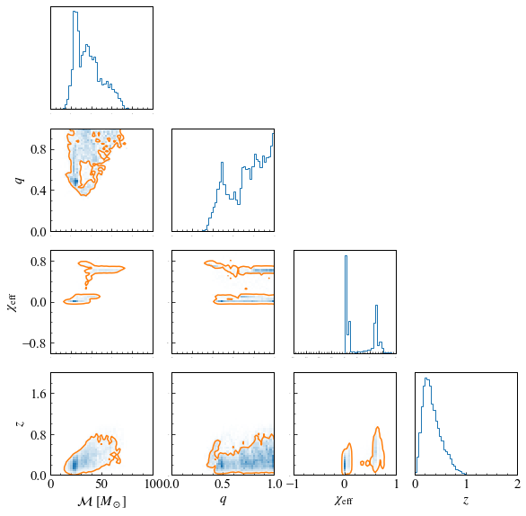
The detection-weighted distribution of binary parameters from this scenario is shown in Figure 1. In the chirp mass distribution, a distinct peak emerges at , as explained. As the field binary, the population is affected by the binary interaction such as the mass transfer, so that the population favors equal-mass binaries and mass ratio . The BH spin under this scenario takes extreme values due to the tidal effect: or Therefore, distribution shows the prominent peak at , while there is an another peak at , which emerges from systems in which only one of the binary star systems is violently rotating. Since the efficiency of the tidal interaction depends on the separation of the binary, binaries with high have very short merger time and the redshift tends to be high. We can see this feature in Fig 1. The subpopulation has higher than the subpopulation.
The redshift distribution shows the peak near , and the probability density decreases with redshift and becomes zero at . This characteristic reflects the sensitivity of our detectors in this work.
II.1.3 Globular Cluster model
As with the isolated field formation channel, the dynamical evolution channel is considered to be a promising pathway for the formation of BBHs. In this scenario, BBHs are formed through dynamical -body interactions in dense stellar circumstances. The high density in the cluster deflects the orbits of the stars to other stars and compact objects. This causes a three-body encounter, where a lighter object in the binary is typically replaced by a heavier object and two massive objects form a binary. When the merger of a BBH occurs, the remnant obtains a kick velocity and it may escape from the star cluster. However, if a remnant BH does not escape from the cluster, it might form a BBH with another BH and can merge with it later. This is called a hierarchical merger scenario and has distinct properties [47].
As a model of the BBH formation in high-density regions, we use the model of [48]. In this model, it was shown that nearly of the BBHs in GC have at least one component that experiences a previous merger. The model is obtained by the -body simulation of a Cluster Monte Carlo (CMC) [49, 50]. CMC procedure can describe the dynamics of individual stars in a cluster, therefore CMC can describe the self-consistent evolution of the stars in the dense cluster. The model incorporates gravitational interactions in the cluster region, such as collisional diffusion, three-body encounters, and tidal stripping.
The authors first constructed 96 models, each with different initial conditions and physical prescriptions. Then, they assigned the weight to each GC model based on the semi-analytic cosmological model for GC formation [51]. With this procedure, they calculated the BBH distributions that originate from GCs for the four BH birth spins cases. In this work, we adopt the model with zero initial BH spin, which is preferred in the previous analysis [27]. The local merger rate for this model is 15 .
II.2 Population Inference
In this work, we assume that BBHs in the universe are formed in three different formation scenarios, the field binary scenario originated from Pop I/II stars, the field binary scenario originated from Pop III stars, and the globular cluster scenario. We then consider a mixed model in which the total merger rate is the sum of the merger rate of each model weighted by the branching fractions with . We apply a hierarchical Bayesian method [26, 52] to estimate the branching fractions by using the BBH events in the GWTC-3 catalog [4]. We consider BBHs in GWTC-3 with the False Alarm Rate less than 1 . This gives us 69 events [25]. We use the posterior/prior samples that are available at Gravitational Wave Open Science Center (GWOSC) [53].
In this work, we don’t estimate the total merger rate itself. Therefore, we marginalize the total coalescence rate of BBHs by assuming log-flat prior [26]. In that case, we can deduce the posterior probability density of branching fraction , given observation set :
| (3) |
The posterior probability density describes the probability density given the observations to infer the unknown population parameter through the binary parameters . A detailed derivation of this equation is given in the Appendix A. The in this equation is a quantity that can be called ”detection efficiency” and will be explained later. is the posterior probability density for estimating the source parameters based on the observed data , and is the prior probability density of the parameter . is the probability density that describes the probability of an event occurring when the hyperparameter is and the true event parameter is . Since the integral on multidimensional parameter space is computationally expensive, we approximate the integral by the discrete sum of the posterior samples of each event available in the LVK GWTC-3 at GWOSC. We have
| (4) |
where denotes the total number of posterior samples used in calculating the sum, and are the LVK posterior samples.
The last term in (3) is given as
| (5) |
where is a probability density distribution that describes the probability that a source with the parameter is generated in -th formation channel, represented by .
Under this formula, we can express as
| (6) |
In this work, we use four parameters for : the source frame chirp mass the mass ratio the effective inspiral spin parameter , and the merger redshift .
The detection efficiency is computed as
| (7) |
where we set
| (8) |
In this equation, is the probability that a binary merger with a true event parameter of can be detected in noisy observations:
| (9) |
where the integration sums up all detectable GW signals. In this work, we set our detection criteria as follows:
-
•
The network SNR exceeds 10.
-
•
Two or more detectors have SNR greater than 4.
In order to evaluate the probability , we first calculate the optimal SNR on the event for -th detector:
| (10) |
where is the Fourier transform of the waveform generated by the binary system with the given parameter , and is the noise power spectral density (PSD) of the -th detector. At the calculation of optimal SNR, extrinsic parameters such as inclination angles are chosen to have maximum SNR for each detector. We use the PyCBC package to generate with the waveform model IMRPhenomD [54, 55], and the actual PSD data from the O3 observing run of LIGO Livingston, LIGO Hanford, and Virgo detectors. After computing in this way, we calculated the optimal network SNR
| (11) |
If optimal SNR does not meet the detection criteria, then we assume that the event cannot be detected, so that . Otherwise, we randomly generate the extrinsic parameters , namely right ascension of the source , declination angle of the source , inclination angle of the source , and polarization angle of the gravitational wave . Those parameters follow the following probability densities: , After obtaining the realization of we calculate the SNR with extrinsic parameters. We finally evaluate as
| (12) |
where denotes the total number of realization of . In this work, we set
For , we construct the kernel density estimator (KDE) from the calculations of the -th astrophysical scenarios. Our population models peak at , which means that our populations tend to have equal-mass binary systems. We note that since is a physical constraint of the parameter, the simple KDE method fails to represent the distribution around . Therefore, we applied the reflection method [56] to the data point . Finally, we calculate the prior distribution which was used by LVK for each BBH candidate.
Now, we can estimate the distribution of . We utilize Dynesty package for plotting the posterior distribution. The Bayes factor between the models and is given as
| (13) |
III Results
III.1 The branching fraction
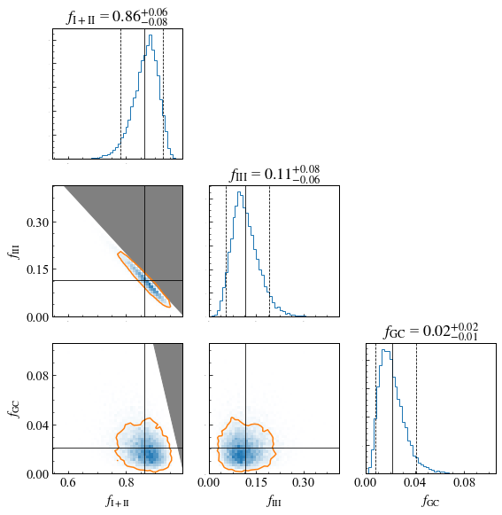
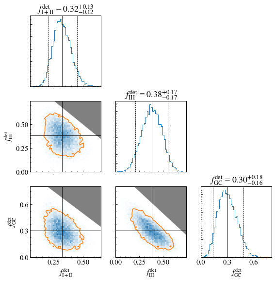
Figure 2 shows the posterior probability density of the fraction for the three BBH population models. In the marginalized one-parameter plots in the diagonal part of the corner plots, we show the median and the 90% credible interval (c.i.) by vertical lines. The gray regions in the 2-dimensional plots are excluded by the constraint . The median and 90% credible interval for the parameters are This implies that the majority of BBHs in the universe have progenitors of field binaries. This result is consistent with their merger rates. It also implies that no contribution from each of the three populations is rejected. In the figure, the anti-correlation between and can be seen.
Figure 3 shows the posterior distribution of the detectable fraction for the models. Here, we define the detectable fraction as
| (14) |
The parameter is proportional to the product of the intrinsic branching fraction and the detection efficiency of the model and normalized so that the sum of detectable fractions becomes unity. The median and 90% credible interval for the parameters are This implies that the contributions of each of the three models are about the same level for the observed events in the catalog. The figure confirm the correlation between This corresponds to the contribution to the observed massive BBH events in GWTC-3. Compared to the intrinsic branching fraction have larger error region. This means that the pathways of BBH formation are obscured under the detector’s sensitivity.
III.2 Model selection
Table 1 shows the result of our model selection. We set the mixed model with consists of Pop I/II field binaries and GC binaries as the reference model, and compare it with other mixed models by using the Bayes factor. We find that the log Bayes factor between Pop I/II+GC+Pop III and Pop I/II+GC is . Therefore, observation results can be explained times more likely by adding the Pop III formation channel to the simple two-channel assumption. The log Bayes factor between Pop I/II-alone model and Pop I/II+GC is . This means that some events in the GWTC-3 cannot be explained as originating from the Pop I/II field binary, implying that the multiple populations behind the BBH mergers. Finally, the log Bayes factor between Pop I/II+Pop III and Pop I/II+GC is . Therefore, even if the contribution to the entire BBH population is small, there should be the contribution of the dynamical mergers in the GWTC-3 events.
| Model mixture | Bayes Factor |
|---|---|
| Pop I/II | |
| Pop I/II GC | |
| Pop I/II Pop III | -2.8 |
| Pop I/II GC Pop III | 2.4 |
III.3 Inferred parameter distribution
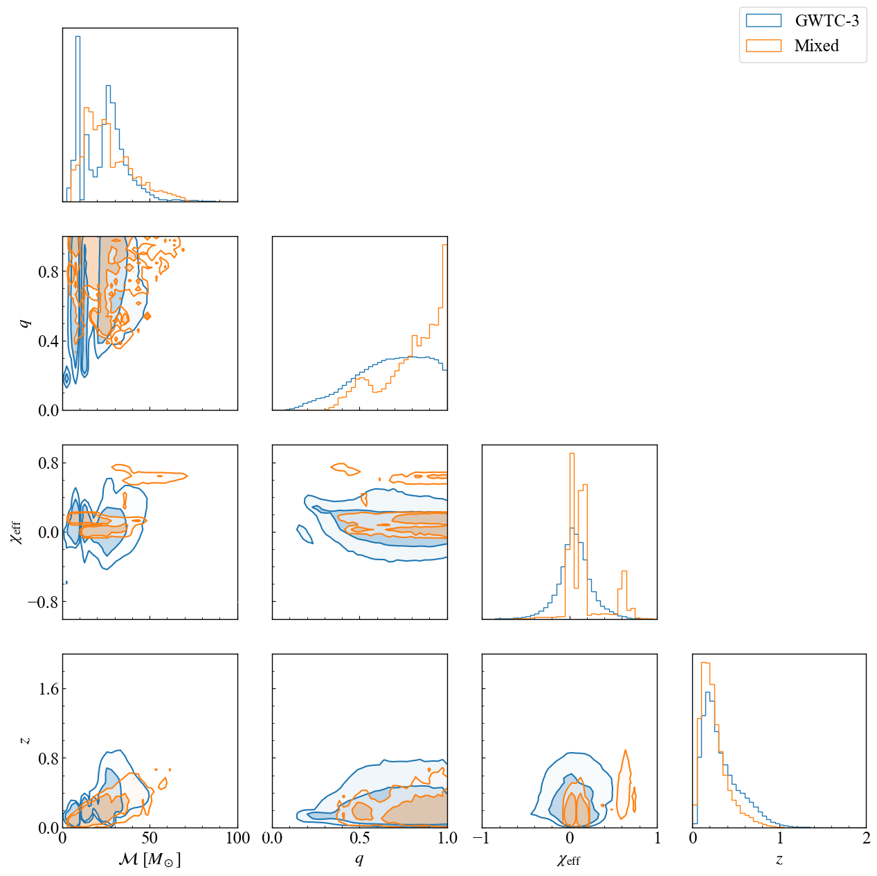
Figure 4 shows the 4-parameter distribution of detectable BBHs when the branching fraction is given by the maximum a posteriori ,
| (15) |
and
| (16) |
The blue plots in Fig. 4 show the stacked distribution of observed BBHs in GWTC-3 taken from the publicly released posterior samples:
| (17) |
Note that has an observational bias, while does not.
Overall, the distribution predicted by the model is consistent with the distribution of the observed events in the GWTC-3. The mixed models with different properties result in a distribution of binary parameters with multiple peaks.
The largest difference in the plot exists in the prediction of peak in the mixed model. Another difference can be seen in the mass ratio parameter, where the mixed model favors while the GWTC-3 events do not show such a preference.
III.3.1 Chirp mass distribution
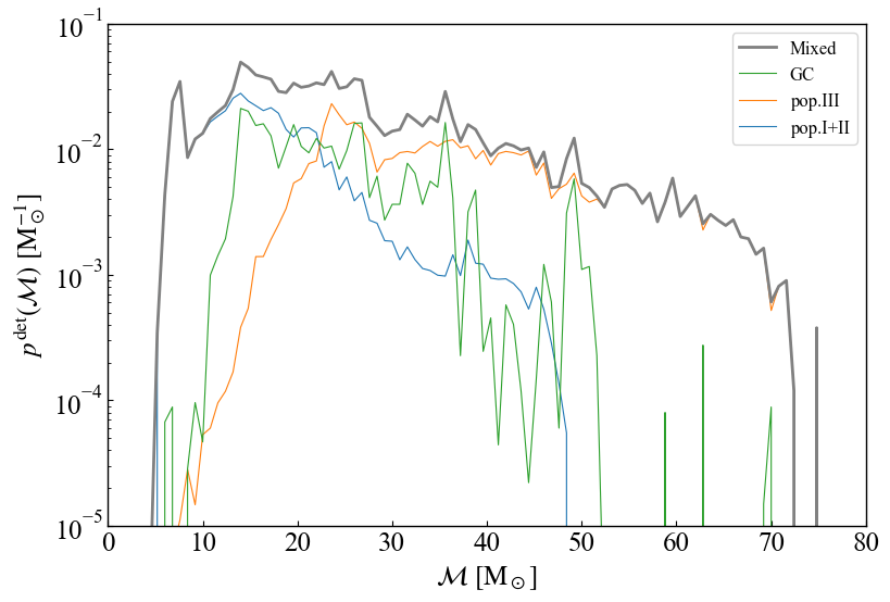
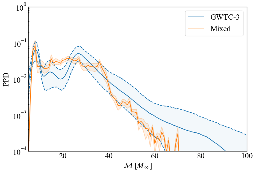
Figure 5 shows the marginal distribution of chirp mass in more detail when the branching fraction are given by Eq. (15). The mixed model of three BBH populations predicts the detectable chirp mass distribution colored in gray in the figure, with the contributions of each model represented by thin lines. In the mixed distribution, the peak from the Pop III star is not prominent. The predicted chirp mass distribution shows a plateau up to and decreases above , rather than two peaks as in the observations.
At the chirp mass , Pop I/II-origin BBH is dominant, while Pop III-origin BBHs dominate the observable BBH. Both GC and Pop I/II contribute from to .
In Figure 6, we compare the observed distribution of chirp mass obtained from GWTC-3 with the mixed-model distribution. For GWTC-3 distribution, we show the distribution estimated by using the adaptive KDE (aKDE) method [57] as LVK did in [25]. The observed distribution is derived as
| (18) |
where the detection efficiency in the denominator is the normalization constant. The kernel bandwidth for GWTC-3 aKDE is optimized for the median value of the individually estimated chirp mass, and the shaded region shows the 90% confidence interval obtained by the boot-strapping method. On the other hand, the mixed-model distribution shows the posterior predictive distribution defined as
| (19) |
The posterior predictive distribution is the estimated distribution for parameter based on our given observations In the calculation of the posterior predictive distribution, we neglect the uncertainty of the population models. This results in narrower credible intervals for mixed distribution compared to that of the GWTC-3 result. In this figure, we find an overall consistency of the marginalized chirp mass distribution. The mixed model reproduces the peak at . It also reproduces the feature of distribution which decreases from to . However, although the observed distribution continues above , the mixed model ends around . The mixed model shows a rather flat distribution between and . There are small peaks at but these are not clear enough to reproduce the peak at in the observed distribution. In the mixed model, there is an additional small peak at although there is no such peak in the observed one.
III.3.2 Spin parameter distribution
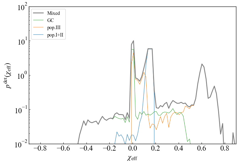
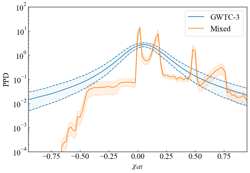
Figure 7 shows the distribution of the effective spin in the mixed model in more detail. We find that the mixed model shows a multi-peak distribution. In the cluster population model, BBHs are formed by the encounter of separately formed BHs, so the spin orientation of each BH does not correlate. This results in the spin distribution of the population being symmetric around zero in the effective spin parameter. We can observe a slightly rightward trend in the detectable distribution of the population due to the detection bias. The field binary channel of Pop I/II stars has a moderately increasing trend of spin, because of accretion from the binary companion. The contribution from Pop III for detectable spin distribution is multi-peaked: one at and the other at
As with the chirp mass distribution, we compare the observed distributions from the GWTC-3 and the mixed model in Figure 8. Again, the kernel bandwidth is optimized to fit the median value of the individually estimated effective spin parameter. Although there is a peak at in the mixed model which is consistent with the observed distribution, we find that the overall feature of the effective spin distribution of the mixed model is inconsistent with the observed one. There are discussions on the efficiency of angular momentum transportation during the evolution of the star. The efficient angular momentum transport pulls the spin out of the core, so if such a mechanism exists, the spin of the remnant BH becomes lower [58]. Each of the models of formation channels utilized in this study employs a sophisticated spin model, but different formation channel models employ different spin models. Therefore, a unified choice of spin prescriptions may allow for model selection that is more consistent with observations.
IV Discussion
We analyzed the latest BBH merger catalog under the assumption of the existence of a population of extremely metal-poor stars. Numerous attempts have been made to clarify the origins of BBHs (For example, [27, 28, 29]). This is the first population inference to spotlight the population with extremely metal-poor populations [10]. The analysis incorporates three binary formation channels: the Pop I/II isolated field formation channel, the Pop III isolated field formation channel, and the GC formation channel. The results with the mixed model favor the domination of the field binary of the intrinsic population of more than 75% with a credibility of 98.5%. The domination by the field population has been reported by a previous study [27], while they also showed that the domination will break down if the natal spin of BH is large. In this study, the natal spin of field BBH is lower than 0.2, so, the result that shows the domination of the Pop I/II population is expected. We also found that in the intrinsic population, the Pop III isolated field population is larger than the GC population. The credibility of GC contributing more significantly than the metal-poor population in the underlying population was about 0.5%. This might aid in placing new restrictions on the star formation rate of Pop III.
The log Bayes factor between the Pop I/II+GC+Pop III model and the Pop I/II+GC model is 2.4. So it is preferred to add the metal-poor population to the formation channel. However, the log Bayes factor between the Pop I/II+Pop III model and the Pop I/II+GC model is -2.8. This suggests that the BBHs from Pop III stars are not influential enough to supplant the dynamical formation scenario in the case of mixed models with two populations. These results may reflect the difference in the spin distribution between the Pop III field scenario and the dynamical scenario. For most events in GWTC-3, the posterior distribution of has an unimodal distribution whose peak is at This feature is in good agreement with that of the GC model. On the other hand, the Pop III BBH model we use in this analysis does not allow the negative . This is one of the reasons that the model selection favors more the GC scenario than the Pop III scenario. In addition, one of the reasons why the mixed model fails to reconstruct the observations well is because we are fitting four parameters simultaneously. Again, the GC model is the only one that can give a large contribution to negative spin in the formation models in this work. However, because of the large spin uncertainty in the observations, there is a non-negligible fraction of negative spin in the posterior samples, even for zero-spin-consistent events. This increases the GC contribution, and as a result, the number of BBH with chirp mass between and increases, making a flat distribution seen in Figs. 5 and 6.
LVK analyzed the redshift evolution of merger rate density [25]. They modeled so that BBH merger rate density evolves with the redshift as and their fiducial conclusion is Using the median value of their merger rate density at the local universe (), we roughly estimate the merger rate density as for Pop I/II, Pop III and GC scenarios, respectively. Therefore, we conclude that the Pop I/II binary should have the local merger rate of , while the Pop III scenario should have . If a detailed rate analysis is to be performed, the analysis should take into account the estimation of the merger rate of each population scenario, which was marginalized in this work. The evaluation of the redshift evolution of the merger rate density is left for future work.
Finally, since Pop III stars are the first stars in the universe, they are formed much earlier than Pop I/II stars. Previous studies show that the peak of the Pop III BBH formation is located at [59, 31]. Therefore, next-generation GW detectors will reveal the nature of the BBH population (such as the redshift-spin correlation) more clearly. The prediction of binary parameter distribution under the mixed model will be informative for the upcoming next-generation GW detectors era.
V Summary
There are many theoretical pathways proposed to explain the formation of BBHs. In this paper, we investigated the BBH formation scenario by taking into account the contribution of the first stars in the universe. We considered three formation channels, Pop I/II isolated field formation channel, Pop III isolated field formation channel, and the dynamical formation channel in GC, and investigated the constraint for the scenarios with the hierarchical Bayesian method by using the observed BBHs events in the GWTC-3.
First, we investigated which combination of the three models is most favored by using the Bayes factor. We set the Pop I/II+GC model as a reference model. The results are summarized in Table 1. We found that the most favored model is the Pop I/II+Pop III+GC model. The log Bayes factor between the Pop I/II+Pop III+GC and the Pop I/II+GC is 2.4. Thus, it is favored to include the Pop III channel to explain the GWTC-3 catalog. However, the log Bayes factor between the Pop I/II+Pop III and Pop I/II+GC is -2.8. This suggests that the GC channel also plays an important role in explaining the GWTC-3 catalog.
Next, we investigated the branching fractions for each model by adopting the mixed model of Pop I/II+Pop III+GC. We found the intrinsic branching fractions, for Pop I/II, Pop III and GC, respectively. Thus, Pop I/II field binaries dominate the intrinsic fraction. On the other hand, we obtained nearly equal contribution for the observed fraction from each channel, i.e. for Pop I/II, Pop III and GC, respectively. Thus, the observed fraction of Pop III is 3 times larger than the intrinsic fraction. Even more noteworthy, the observed fraction of GC is about 0.3 even if the intrinsic fraction is only 0.02. These are due to the difference in the detection efficiency for each channel. Since the Pop I/II field binaries are dominated by low-mass BBHs, the detection efficiency becomes lower compared to Pop III and GC. In the Pop III channel, since the fraction of BBHs that merge in the observable redshift is small, the detection efficiency becomes lower compared to GC.
Finally, we investigated the mass and spin distribution of the best-fit Pop I/II+Pop III+GC mixed model. We found that the mixed model reproduced the peak of chirp mass distribution at . However, the mixed model shows a rather flat distribution between and and can not reproduce the peak around . It show the feature of distribution which decreases from to which agree with the observed distribution. However, although the observed distribution continues above , the mixed model ends around .
In this work, we used only one representative model for each formation channel. However, even for the same channel, the distribution of the BBH parameters can differ significantly due to different physical assumptions. We want to take into account different models for each channel in future work.
Acknowledgement
M. I. was supported by Forefront Physics and Mathematics Program to Drive Transformation (FoPM), a World-leading Innovative Graduate Study (WINGS) Program, the University of Tokyo. This research has made use of data obtained from the Gravitational Wave Open Science Center (gwosc.org), a service of LIGO Laboratory, the LIGO Scientific Collaboration, the Virgo Collaboration, and KAGRA. LIGO Laboratory and Advanced LIGO are funded by the United States National Science Foundation (NSF) as well as the Science and Technology Facilities Council (STFC) of the United Kingdom, the Max-Planck-Society (MPS), and the State of Niedersachsen/Germany for support of the construction of Advanced LIGO and construction and operation of the GEO600 detector. Additional support for Advanced LIGO was provided by the Australian Research Council. Virgo is funded, through the European Gravitational Observatory (EGO), by the French Centre National de Recherche Scientifique (CNRS), the Italian Istituto Nazionale di Fisica Nucleare (INFN) and the Dutch Nikhef, with contributions by institutions from Belgium, Germany, Greece, Hungary, Ireland, Japan, Monaco, Poland, Portugal, Spain. KAGRA is supported by Ministry of Education, Culture, Sports, Science and Technology (MEXT), Japan Society for the Promotion of Science (JSPS) in Japan; National Research Foundation (NRF) and Ministry of Science and ICT (MSIT) in Korea; Academia Sinica (AS) and National Science and Technology Council (NSTC) in Taiwan. This work was supported by JSPS Grant-inAid for Scientific Research on Innovative Areas 2905: JP17H06358, JP17H06361 and JP17H06364, JSPS Core-to-Core Program A. Advanced Research Networks, JSPS Grant-in-Aid for Transformative Research Areas (A) 20A203: JP20H05854, the joint research program of the Institute for Cosmic Ray Research, University of Tokyo.
T. K. acknowledges support from JSPS KAKENHI Grant Numbers JP21K13915 and JP22K03630.
Appendix A Hierarchical Bayesian Analysis
Here, we describe a summary of the hierarchical Bayesian analysis method. In a Bayesian manner, Given a set of data from observation, one can calculate the posterior distribution for population parameter , , as
| (20) |
where is the prior distribution for the population parameter . If we assume that all events are independent of each other, this probability can be expressed as
| (21) |
where denotes the observation data of -th event. For each GW event, we estimate the source parameter such as masses, and we denote this by The probability of detecting the GW event from population parameter can be described by marginalizing over :
| (22) |
Since we have the detection, must be ’detectable.’ In other words, must pass the detection criteria. Therefore, the normalization for equation (22) must be
| (23) |
where the integral domain is the entire satisfying detection criteria. This requires a parameter so-called ’detection efficiency’ as a normalization factor:
| (24) |
where is the probability that a gravitational wave from a binary system with binary parameter is observed by the detectors. With the normalization factor, the equation to assess becomes
| (25) |
For every event in the GWTC-3, LVK collaboration estimates the source parameter on it, applying Bayesian analysis [4]. Hence, can be converted to by applying Bayes’ theorem:
| (26) |
Finally, we have
| (27) |
References
- Abbott et al. [2016] B. P. Abbott et al. (LIGO Scientific Collaboration and Virgo Collaboration), Phys. Rev. Lett. 116, 061102 (2016), arXiv:1602.03837 [gr-qc] .
- Abbott et al. [2019] B. P. Abbott et al. (LIGO Scientific Collaboration and Virgo Collaboration), Physical Review X 9, 031040 (2019), arXiv:1811.12907 [astro-ph.HE] .
- Abbott et al. [2021] R. Abbott, T. Abbott, F. Acernese, K. Ackley, C. Adams, N. Adhikari, R. Adhikari, V. Adya, C. Affeldt, D. Agarwal, et al., arXiv e-prints , arXiv:2108.01045 (2021), arXiv:2108.01045 [gr-qc] .
- Abbott et al. [2023a] R. Abbott et al. (LIGO Scientific Collaboration, Virgo Collaboration, and KAGRA Collaboration), Physical Review X 13, 041039 (2023a), arXiv:2111.03606 [gr-qc] .
- Paczynski [1976] B. Paczynski, in Structure and Evolution of Close Binary Systems, Vol. 73, edited by P. Eggleton, S. Mitton, and J. Whelan (1976) p. 75.
- Bethe and Brown [1998] H. A. Bethe and G. E. Brown, Astrophys. J. 506, 780 (1998), arXiv:astro-ph/9802084 [astro-ph] .
- Röpke and De Marco [2023] F. K. Röpke and O. De Marco, Living Reviews in Computational Astrophysics 9, 2 (2023), arXiv:2212.07308 [astro-ph.SR] .
- van den Heuvel et al. [2017] E. P. J. van den Heuvel, S. F. Portegies Zwart, and S. E. de Mink, mnras 471, 4256 (2017), arXiv:1701.02355 [astro-ph.SR] .
- Neijssel et al. [2019] C. J. Neijssel, A. Vigna-Gómez, S. Stevenson, J. W. Barrett, S. M. Gaebel, F. S. Broekgaarden, S. E. de Mink, D. Szécsi, S. Vinciguerra, and I. Mandel, mnras 490, 3740 (2019), arXiv:1906.08136 [astro-ph.SR] .
- Kinugawa et al. [2014] T. Kinugawa, K. Inayoshi, K. Hotokezaka, D. Nakauchi, and T. Nakamura, mnras 442, 2963 (2014), arXiv:1402.6672 [astro-ph.HE] .
- Abel et al. [2002] T. Abel, G. L. Bryan, and M. L. Norman, Science 295, 93 (2002), arXiv:astro-ph/0112088 [astro-ph] .
- Tanikawa et al. [2020] A. Tanikawa, T. Yoshida, T. Kinugawa, K. Takahashi, and H. Umeda, mnras 495, 4170 (2020), arXiv:1906.06641 [astro-ph.HE] .
- Bromm and Larson [2004] V. Bromm and R. B. Larson, araa 42, 79 (2004), arXiv:astro-ph/0311019 [astro-ph] .
- Ekström et al. [2008] S. Ekström, G. Meynet, C. Chiappini, R. Hirschi, and A. Maeder, aap 489, 685 (2008), arXiv:0807.0573 [astro-ph] .
- Marigo et al. [2003] P. Marigo, C. Chiosi, and R. P. Kudritzki, aap 399, 617 (2003), arXiv:astro-ph/0212057 [astro-ph] .
- Kulkarni et al. [1993] S. R. Kulkarni, P. Hut, and S. McMillan, Nature (London) 364, 421 (1993).
- Rodriguez et al. [2015] C. L. Rodriguez, M. Morscher, B. Pattabiraman, S. Chatterjee, C.-J. Haster, and F. A. Rasio, Physical Review Letters 115, 051101 (2015), arXiv:1505.00792 [astro-ph.HE] .
- Di Carlo et al. [2020] U. N. Di Carlo, M. Mapelli, N. Giacobbo, M. Spera, Y. Bouffanais, S. Rastello, F. Santoliquido, M. Pasquato, A. Ballone, A. A. Trani, S. Torniamenti, and F. Haardt, MNRAS 498, 495 (2020), arXiv:2004.09525 [astro-ph.HE] .
- de Mink and Mandel [2016] S. E. de Mink and I. Mandel, mnras 460, 3545 (2016), arXiv:1603.02291 [astro-ph.HE] .
- Antonini et al. [2017] F. Antonini, S. Toonen, and A. S. Hamers, apj 841, 77 (2017), arXiv:1703.06614 [astro-ph.GA] .
- Bartos et al. [2017] I. Bartos, B. Kocsis, Z. Haiman, and S. Márka, Astrophys. J. 835, 165 (2017), arXiv:1602.03831 [astro-ph.HE] .
- Yang et al. [2019] Y. Yang, I. Bartos, V. Gayathri, K. E. S. Ford, Z. Haiman, S. Klimenko, B. Kocsis, S. Márka, Z. Márka, B. McKernan, and R. O’Shaughnessy, Phys. Rev. Lett. 123, 181101 (2019), arXiv:1906.09281 [astro-ph.HE] .
- Bird et al. [2016] S. Bird, I. Cholis, J. B. Muñoz, Y. Ali-Haïmoud, M. Kamionkowski, E. D. Kovetz, A. Raccanelli, and A. G. Riess, Phys. Rev. Lett. 116, 201301 (2016), arXiv:1603.00464 [astro-ph.CO] .
- Mandel and Broekgaarden [2022] I. Mandel and F. S. Broekgaarden, Living Reviews in Relativity 25, 1 (2022), arXiv:2107.14239 [astro-ph.HE] .
- Abbott et al. [2023b] R. Abbott et al. (LIGO Scientific Collaboration and VIRGO Collaboration and KAGRA Collaboration), Physical Review X 13, 011048 (2023b), arXiv:2111.03634 [astro-ph.HE] .
- Mandel et al. [2019] I. Mandel, W. M. Farr, and J. R. Gair, mnras 486, 1086 (2019), arXiv:1809.02063 [physics.data-an] .
- Zevin et al. [2021] M. Zevin, S. S. Bavera, C. P. L. Berry, V. Kalogera, T. Fragos, P. Marchant, C. L. Rodriguez, F. Antonini, D. E. Holz, and C. Pankow, Astrophys. J. 910, 152 (2021), arXiv:2011.10057 [astro-ph.HE] .
- Franciolini and Pani [2022] G. Franciolini and P. Pani, Phys. Rev. D 105, 123024 (2022), arXiv:2201.13098 [astro-ph.HE] .
- Gayathri et al. [2023] V. Gayathri, D. Wysocki, Y. Yang, V. Delfavero, R. O’Shaughnessy, Z. Haiman, H. Tagawa, and I. Bartos, apjl 945, L29 (2023), arXiv:2301.04187 [gr-qc] .
- Hartwig et al. [2016] T. Hartwig, M. Volonteri, V. Bromm, R. S. Klessen, E. Barausse, M. Magg, and A. Stacy, mnras 460, L74 (2016), arXiv:1603.05655 [astro-ph.GA] .
- Kinugawa et al. [2020] T. Kinugawa, T. Nakamura, and H. Nakano, mnras 498, 3946 (2020), arXiv:2005.09795 [astro-ph.HE] .
- Belczynski et al. [2017] K. Belczynski, T. Ryu, R. Perna, E. Berti, T. L. Tanaka, and T. Bulik, mnras 471, 4702 (2017), arXiv:1612.01524 [astro-ph.HE] .
- Santoliquido et al. [2023] F. Santoliquido, M. Mapelli, G. Iorio, G. Costa, S. C. O. Glover, T. Hartwig, R. S. Klessen, and L. Merli, mnras 524, 307 (2023), arXiv:2303.15515 [astro-ph.GA] .
- Punturo et al. [2010] M. Punturo et al., Classical and Quantum Gravity 27, 194002 (2010).
- Liu and Bromm [2020] B. Liu and V. Bromm, apjl 903, L40 (2020), arXiv:2009.11447 [astro-ph.GA] .
- Belczynski et al. [2020] K. Belczynski et al., aap 636, A104 (2020), arXiv:1706.07053 [astro-ph.HE] .
- Belczynski et al. [2002] K. Belczynski, T. Bulik, and V. Kalogera, apjl 571, L147 (2002), arXiv:astro-ph/0204416 [astro-ph] .
- Belczynski et al. [2008] K. Belczynski, V. Kalogera, F. A. Rasio, R. E. Taam, A. Zezas, T. Bulik, T. J. Maccarone, and N. Ivanova, apjs 174, 223 (2008), arXiv:astro-ph/0511811 [astro-ph] .
- Madau and Fragos [2017] P. Madau and T. Fragos, Astrophys. J. 840, 39 (2017), arXiv:1606.07887 [astro-ph.GA] .
- Spruit [2002] H. C. Spruit, aap 381, 923 (2002), arXiv:astro-ph/0108207 [astro-ph] .
- Hosokawa et al. [2011] T. Hosokawa, K. Omukai, N. Yoshida, and H. W. Yorke, Science 334, 1250 (2011), arXiv:1111.3649 [astro-ph.CO] .
- Marigo et al. [2001] P. Marigo, L. Girardi, C. Chiosi, and P. R. Wood, aap 371, 152 (2001), arXiv:astro-ph/0102253 [astro-ph] .
- Hurley et al. [2002] J. R. Hurley, C. A. Tout, and O. R. Pols, mnras 329, 897 (2002), arXiv:astro-ph/0201220 [astro-ph] .
- de Souza et al. [2011] R. S. de Souza, N. Yoshida, and K. Ioka, aap 533, A32 (2011), arXiv:1105.2395 [astro-ph.CO] .
- Inayoshi et al. [2016] K. Inayoshi, K. Kashiyama, E. Visbal, and Z. Haiman, mnras 461, 2722 (2016), arXiv:1603.06921 [astro-ph.GA] .
- Kinugawa et al. [2021] T. Kinugawa, T. Nakamura, and H. Nakano, mnras 504, L28 (2021), arXiv:2103.00797 [astro-ph.HE] .
- Gerosa and Berti [2017] D. Gerosa and E. Berti, Phys. Rev. D 95, 124046 (2017), arXiv:1703.06223 [gr-qc] .
- Rodriguez et al. [2019] C. L. Rodriguez, M. Zevin, P. Amaro-Seoane, S. Chatterjee, K. Kremer, F. A. Rasio, and C. S. Ye, Phys. Rev. D 100, 043027 (2019), arXiv:1906.10260 [astro-ph.HE] .
- Joshi et al. [2000] K. J. Joshi, F. A. Rasio, and S. Portegies Zwart, Astrophys. J. 540, 969 (2000), arXiv:astro-ph/9909115 [astro-ph] .
- Pattabiraman et al. [2013] B. Pattabiraman, S. Umbreit, W.-k. Liao, A. Choudhary, V. Kalogera, G. Memik, and F. A. Rasio, apjs 204, 15 (2013), arXiv:1206.5878 [astro-ph.IM] .
- El-Badry et al. [2019] K. El-Badry, E. Quataert, D. R. Weisz, N. Choksi, and M. Boylan-Kolchin, mnras 482, 4528 (2019), arXiv:1805.03652 [astro-ph.GA] .
- Thrane and Talbot [2019] E. Thrane and C. Talbot, pasa 36, e010 (2019), arXiv:1809.02293 [astro-ph.IM] .
- Abbott et al. [2023c] R. Abbott et al. (LIGO Scientific Collaboration and Virgo Collaboration and KAGRA Collaboration), apjs 267, 29 (2023c), arXiv:2302.03676 [gr-qc] .
- Husa et al. [2016] S. Husa, S. Khan, M. Hannam, M. Pürrer, F. Ohme, X. J. Forteza, and A. Bohé, Phys. Rev. D 93, 044006 (2016), arXiv:1508.07250 [gr-qc] .
- Khan et al. [2016] S. Khan, S. Husa, M. Hannam, F. Ohme, M. Pürrer, X. J. Forteza, and A. Bohé, Phys. Rev. D 93, 044007 (2016), arXiv:1508.07253 [gr-qc] .
- Silverman [1986] B. W. Silverman, Density estimation for statistics and data analysis (1986).
- Sadiq et al. [2022] J. Sadiq, T. Dent, and D. Wysocki, Phys. Rev. D 105, 123014 (2022), arXiv:2112.12659 [gr-qc] .
- Maeder and Meynet [2000] A. Maeder and G. Meynet, araa 38, 143 (2000), arXiv:astro-ph/0004204 [astro-ph] .
- Tanikawa et al. [2021] A. Tanikawa, H. Susa, T. Yoshida, A. A. Trani, and T. Kinugawa, Astrophys. J. 910, 30 (2021), arXiv:2008.01890 [astro-ph.HE] .