Influence Minimization via Blocking Strategies

Abstract

We study the influence minimization problem: given a graph $G$ and a seed set $S$, blocking at most $b$ nodes or $b$ edges such that the influence spread of the seed set is minimized. This is a pivotal yet underexplored aspect of network analytics, which can limit the spread of undesirable phenomena in networks, such as misinformation and epidemics. Given the inherent NP-hardness of the problem under the IC and LT models, previous studies have employed greedy algorithms and Monte Carlo Simulations for its resolution. However, existing techniques become cost-prohibitive when applied to large networks due to the necessity of enumerating all the candidate blockers and computing the decrease in expected spread from blocking each of them. This significantly restricts the practicality and effectiveness of existing methods, especially when prompt decision-making is crucial. In this paper, we propose the AdvancedGreedy algorithm, which utilizes a novel graph sampling technique that incorporates the dominator tree structure. We find that AdvancedGreedy can achieve a $(1-1/e-\epsilon)$-approximation in the problem under the LT model. Experimental evaluations on real-life networks reveal that our proposed algorithms exhibit a significant enhancement in efficiency, surpassing the state-of-the-art algorithm by three orders of magnitude, while achieving high effectiveness.

Keywords: Influence Spread, Influence Minimization, Misinformation, Epidemic Control, Social Networks

1 Introduction

In today’s hyper-connected world, the concept of influence maximization, which aims to target a select group of individuals in order to maximize the spread of influence (Domingos and Richardson 2001, Kempe et al. 2003), has long been a focal point of research due to its commercial potential in various industries such as marketing, finance, education, etc (e.g., Chen et al. 2010, Banerjee et al. 2013, Yadav et al. 2017, Günneç et al. 2020, Wu et al. 2020, Raghavan and Zhang 2022, Eckles et al. 2022). However, a lesser-explored yet equally critical counterpart to this problem is the influence minimization problem. This problem involves identifying a specific set of nodes (or edges) in a network in order to minimize the spread of influence, particularly when some forms of influence are detrimental. Let us provide the following two examples to illustrate the importance of minimizing the spread of influence.

Managing Misinformation Propagation. In the era of rapid information dissemination and the prevalence of social media, the proliferation of false news and misinformation has emerged as a major societal concern and is regarded as one of the most significant global economic risks (World Economic Forum 2022). The dissemination of false information or unverified rumors can lead to various adverse effects, such as economic damage, substantial disruption, and widespread panic. For example, a false tweet claiming that Barack Obama was injured in an explosion at the White House led to a significant decline of $136.5 billion in the stock market (Gentzkow 2017). In fact, misinformation, such as rumors, spreads faster than true news in social networks (Doerr et al. 2012, Vosoughi et al. 2018) and tends to form more clusters than positive information (Johnson et al. 2020). Therefore, it is crucial to identify influential nodes or edges within the social network to restrict the dissemination of such misinformation and mitigate the potential negative consequences.

Enhancing Epidemic Control. The outbreak of infectious diseases poses formidable challenges to public health systems worldwide, demanding swift and strategic intervention to limit transmission. The emergence and rapid spread of infectious agents can swiftly overwhelm healthcare infrastructures, jeopardizing the health and well-being of communities on a global scale. For example, COVID-19 is being attributed as the final factor leading to the breakdown of the United Kingdom’s healthcare system (McLellan and Abbasi 2022). In such scenarios, timely responses become paramount to mitigate the potential cascading effects on morbidity, mortality, and socio-economic stability. The adverse effects of infectious disease outbreaks underscore the importance of harnessing innovative solutions that can efficiently identify critical nodes or edges within transmission networks and guide swift containment measures.

The above examples highlight the urgent need for effective solutions to the influence minimization problem. The problem can be formulated as follows (Wang et al. 2013, Yan et al. 2020): a social network (or a transmission network) is modeled as a graph where nodes represent individuals and edges represent connections or relationships between them. The propagation of influence (e.g., fake news or diseases) in a network follows a diffusion model, such as the independent cascade (IC) model or linear threshold (LT) model (Kempe et al. 2003). Given a graph $G$, a seed set $S$, and a budget $b$, the objective of the influence minimization problem is to identify a set $B^{*}$ consisting of at most $b$ nodes (or $b$ edges) that minimizes the expected number of nodes activated by the seeds $S$ (referred to as the expected influence spread) under a specific diffusion model.

Existing research has explored various methods to tackle the influence minimization problem (e.g., Kimura et al. 2008, Wang et al. 2013, Kuhlman et al. 2013, Yan et al. 2020, Wang et al. 2020). However, a common limitation observed in these approaches is their high time complexity. For instance, the processing time required for the Wiki-Vote network (7K nodes and 103K edges) exceeds three days when using these methods. This significantly hinders their applicability to large networks and real-time scenarios where prompt decision-making is essential for effective intervention (Zareie and Sakellariou 2021). From a pragmatic perspective, it is impractical for an algorithm to require a longer duration to discover a solution that minimizes influence spread compared to the actual time required for influence to propagate.

To address the limitation, we present novel and efficient algorithms that tackle the influence minimization problem. Our algorithms address the scalability issues encountered by existing solutions, providing a significant leap forward in terms of computational speed and adaptability to large-scale real-world networks. Our proposed algorithms showcase an unprecedented speedup, outperforming existing methods by an astonishing three orders of magnitude. In addition, we conduct an exhaustive series of real-data experiments to evaluate the efficacy and applicability of our proposed algorithms in a variety of scenarios. In the following section, we discuss the various technical challenges encountered and the corresponding contributions in detail.

1.1 Main Technical Challenges

There are several technical challenges in influence minimization problems. First, the influence minimization problem is NP-hard (Theorems 1). Consequently, the state-of-the-art algorithms employ a greedy framework to select the blockers (Budak et al. 2011, Wang et al. 2013), which has proven to be superior to alternative heuristics proposed in previous studies (e.g, Rita et al. 2000, Newman et al. 2002, Yan et al. 2020). However, in contrast to the influence maximization problem, we demonstrate that the expected spread function in the influence minimization problem does not exhibit supermodularity (Theorem 8) and we prove the problem is APX-hard under the IC model (Theorem 9). As a result, existing greedy solutions may not possess an approximation guarantee.

Second, similar to the influence maximization problem, an essential component of the greedy algorithm involves the computation of the influence spread from the seeds, a problem known to be #P-hard (Chen et al. 2010). Rather than relying on an exact algorithm, state-of-the-art solutions for estimating influence spread in diffusion models utilize Monte-Carlo Simulations (Ishihata and Sato 2011, Ohsaka et al. 2014, Zhang et al. 2014). In contrast to the influence maximization problem, the influence minimization problem incorporates an additional step, which involves the computation of the reduction in expected influence spread that would occur by blocking a particular node or edge (detailed in Section 4.1). In order to accomplish this, the current algorithms must iterate through all potential nodes or edges. Given the presence of an overwhelming number of potential candidate nodes or edges that could be blocked, the implementation of these methods becomes economically unfeasible when applied to larger graphs.

1.2 Our Contributions

In this paper, we first present that the influence minimization problem is NP-hard and that the problem under the IC model is APX-hard unless P=NP, which has not been proved by previous scholars. We further find that the expected spread function is supermodular for the problem under the LT model, which enables us to leverage the greedy algorithm to achieve a $(1-1/e-\epsilon)$-approximation.

We then tackle the issue of scalability by introducing a novel algorithm, namely the AdvancedGreedy algorithm. This algorithm exhibits a remarkable increase in speed by several orders of magnitude compared to all preexisting greedy algorithms while maintaining their efficacy. The efficiency of our algorithm is enhanced through the simultaneous computation of the expected influence spread reduction for each candidate node and edges. This is achieved by employing an almost linear scan of each sampled graph. The central concept underlying our algorithm is the utilization of the dominator tree for the computation of the expected reduction in expected influence spread. This novel approach has not yet been employed in the context of influence-related problems. We prove that the decrease of the expected influence spread from a blocked node is decided by the subtrees rooted in the dominator trees that are generated from the sampled graphs (Theorem 5), and we establish that the edge version problem can be effectively solved by transforming it into the node version problem (Theorems 6 and 7). Hence, rather than relying on Monte Carlo Simulations, we can effectively calculate the expected reduction in influence spread by employing sampled graphs and their dominator trees. We also prove the estimation result is theoretically guaranteed given a certain number of samples (Theorem 4). Our algorithm demonstrates remarkable scalability, enabling it to easily apply to networks comprising millions of nodes and edges. Furthermore, we prove the AdvancedGreedy algorithm can achieve a $(1-1/e-\epsilon)$-approximation for both node and edge blocking problems under the LT model.

In addition, for the problem under the IC model, since the problem is APX-hard, we further propose a novel heuristic. When employing the node-blocking strategy, it is evident that if the budget is unlimited, all out-neighbors of the seeds will be blocked. However, the current greedy algorithm may select nodes that are not the out-neighbors as blockers, potentially overlooking crucial candidates. Considering this, we propose a new heuristic, named the GreedyReplace algorithm, focusing on the relationships among candidate blockers. Specifically, we begin by restricting the pool of candidate blockers to the out-neighbors of the blocking nodes. Subsequently, we adopt a greedy strategy to replace these blockers with alternative nodes, should the expected influence spread diminish. This algorithm demonstrates superior performance.

We conduct extensive experiments on $8$ real-life datasets with varying scales, features, and diffusion models. Our proposed algorithms are compared with the state-of-the-art algorithm, namely the greedy algorithm with Monte-Carlo Simulations (Budak et al. 2011, Wang et al. 2013, Yan et al. 2020), as well as other heuristics. Our experiments show that (a) our AdvancedGreedy algorithm exhibits significantly enhanced speed when compared to existing algorithms, surpassing them by a factor of more than three orders of magnitude, (b) our GreedyReplace algorithm demonstrates superior effectiveness, as evidenced by its ability to achieve smaller influence spreads while maintaining comparable efficiency to our AdvancedGreedy algorithm.

Overall, our research makes significant strides in the realm of influence minimization problems, providing innovative solutions that overcome existing limitations. Our proposed algorithms outperform existing methods by three orders of magnitude in terms of speed. By achieving such remarkable computational efficiency, our approach opens new avenues for managing large-scale networks and real-time scenarios, enabling faster and more proactive responses to potential crises.

The remainder of this paper is structured as follows: In Section 2, we present a comprehensive review of the related literature. Section 3 offers a formal definition of the influence minimization problem, introduces the most advanced existing algorithm, and establishes the NP-hard nature of the influence minimization problem. Section 4 provides a detailed description of how we calculate the reduction of expected influence spread. Section 5 introduces our proposed algorithms and their implementation. Section 6 outlines the experiment and presents the results obtained from applying our approach to real-life graphs. Finally, Section 7 concludes this work, summarizing the main contributions and discussing future research directions.

2 Related Work

This section provides an overview of three streams of literature that are relevant to our research: the influence maximization problem, the influence minimization problem, and the computation of expected influence spread.

The Influence Maximization Problem. The studies of influence maximization are surveyed in Li et al. (2018), Banerjee et al. (2020) and Aghaee et al. (2021). Domingos and Richardson (2001) are the first to study the influence between individuals for marketing in social networks. Kempe et al. (2003) initially formulate this problem as a discrete optimization problem, referred to as the influence maximization problem. They introduce the IC and LT diffusion models and propose a greedy algorithm that achieves a $(1-1/e)$-approximation ratio due to the submodularity of the function under these models. Subsequently, some researchers have proposed advanced approaches, such as reverse sampling (Borgs et al. 2014, Tang et al. 2014, 2015) , to enhance the scalability and effectiveness of the algorithms. Other researchers have explored strategies to maximize influence in practical scenarios that may involve domain-specific challenges, such as inability to conduct intervention (Yadav et al. 2017), costly network information (Eckles et al. 2022), partial feedback (Tang and Yuan 2020), minimum total amount of inducements (Han et al. 2019, Günneç et al. 2020), capacity constraints (Zhang et al. 2023), etc.

In contrast to prior research, the objective of this paper is to make a contribution to the field of influence minimization problem, which presents unique challenges that cannot be addressed using existing solutions for influence maximization problem. While the influence minimization problem may appear to be the inverse of the influence maximization problem, it actually entails additional complexities. Specifically, it requires the estimation of the expected reduction in influence spread resulting from the blocking of certain nodes or edges.

The Influence Minimization Problem. Compared with the influence maximization problem, there are fewer studies on minimizing the spread of influence, as surveyed in Zareie and Sakellariou (2021). In general, there are two main strategies that can be employed to solve the influence minimization problem. The first strategy involves blocking (or removing) specific nodes or edges to minimize the overall impact of influence (e.g., Kimura et al. 2008, Wang et al. 2013, Yao et al. 2015, Yan et al. 2020). The second strategy, known as the counterbalance strategy, involves the dissemination of positive information throughout the network (e.g., Budak et al. 2011, Lee et al. 2019, Tong et al. 2020, Manouchehri et al. 2021). By increasing people’s awareness and providing them with positive content, the negative influence is reduced. This methodology is predominantly employed to address the dissemination of misinformation. Our papers fall within the first category.

Motivated by the feasibility of structure change for influence-related studies (Nie et al. 2016, Wang et al. 2016, Sun et al. 2020), most works have focused on utilizing the blocking strategy (i.e., blocking nodes or edges) to minimize the influence spread. Intuitively, simple heuristics that rely on network structure can be employed to identify influential nodes to restrict the spread of influence. For instance, one commonly used heuristic is the degree-based heuristic (Rita et al. 2000, Newman et al. 2002, Shah and Zaman 2011, 2016). Another approach involves considering the betweenness and out-degree heuristics (Yao et al. 2015). However, subsequent studies have shown that these simple degree-based heuristic methods are comparatively less effective than greedy heuristics (Wang et al. 2013, Yan et al. 2020). Consequently, different greedy algorithms have been proposed to address the influence minimization problem by blocking nodes or edges under various diffusion models (Kimura et al. 2008, Wang et al. 2013, Kuhlman et al. 2013, Yan et al. 2020, Milling et al. 2015, Nguyen et al. 2020, Hoffmann et al. 2020).

However, a prevalent constraint observed in these methodologies is their limited ability to scale effectively when applied to large networks (Zareie and Sakellariou 2021). Even the most advanced greedy approach requires the enumeration of all candidate nodes to calculate the reduction in expected influence spread. Consequently, the computational speed of their solutions often falls short in dealing with real-time scenarios, where quick decisions are crucial for successful intervention. In this paper, we develop a computationally efficient approach that maintains its effectiveness when compared to existing algorithms for minimizing influence spread. Specifically, we consider two fundamental blocking strategies: node blocking and edge blocking. Additionally, we also consider two distinct diffusion models, namely the LT model and the IC model.

The Computation of the Expected Spread. An essential aspect of the influence minimization problem involves the estimation of the expected spread from the seeds, which has been proved to be #P-hard under IC model (Chen et al. 2010). Kempe et al. (2003) first propose to use the Monte-Carlo Simulations (MCS) to compute the expected influence spread, which repeats simulations until a tight estimation is obtained. In a subsequent study, Borgs et al. (2014) propose Reverse Influence Sampling (RIS), which is now widely used in the influence maximization problem. Tang et al. (2015) enhance the existing methods by reducing the number of samples for RIS. Subsequently, Maehara et al. (2017) propose the first algorithm to compute the exact influence spread under the IC model. However, its applicability is limited to small graphs containing a few hundred edges.

However, as discussed later in Section 4.1, we find that MCS and RIS are not applicable to our problem. This is because influence minimization problems require repetitive computation of the expected decrease in influence spread for each potential blocked node/edge. We contribute to this stream of literature by introducing the dominator tree when calculating the reduction of expected influence spread. Our computation of the expected influence spread on sampled graphs can return the spread decrease of every candidate node/edge simultaneously, which avoids redundant computations compared with MCS or RIS.

3 Preliminaries

We consider a directed graph $G=(V,E)$, where $V$ is the set of $n$ nodes (individuals), and $E$ is the set of $m$ directed edges (influence relations between node pairs). We use $V(G)$ (resp. $E(G)$) to represent the set of nodes (resp. edges) in $G$, and $p_{u,v}$ denotes the probability that node $u$ activates node $v$. Let $G[V]$ denote the induced subgraph by the node set $V$. $N^{in}_{v}$ (resp. $N^{out}_{v}$) is the in-neighbor (resp. out-neighbor) set of $v$ in $G$. The in-degree (resp. out-degree) of $v$ in graph $G$, is denoted by $d^{in}_{v}=|N^{in}_{v}|$ (resp. $d^{out}_{v}=|N^{out}_{v}|$). We use $Pr[x]$ to denote the probability if $x$ is true and $\mathbb{E}[x]$ to denote the expectation of variable $x$. Table A1 in the online appendix summarizes the notations.

3.1 Diffusion Model

Following the existing studies on influence minimization (Budak et al. 2011, Wang et al. 2013, Tang et al. 2014), we focus on the two widely-studied diffusion models, namely IC model and LT model (Kempe et al. 2003), which capture the “word-of-mouth” effects, i.e., each node’s tendency to become active increases monotonically as more of its neighbors become active. They both assume each directed edge $(u,v)$ in the graph $G$ has a propagation probability $p_{u,v}\in[0,1]$, i.e., the probability that the node $u$ activates the node $v$ after $u$ is activated. In both two diffusion models, each node has two states: inactive or active. We say a node is activated if it becomes active by the influence spread (e.g., fake news or diseases), and an active node will not be inactivated during the diffusion process.

LT model. LT model is proposed by Granovetter (1978) and Schelling (2006) to capture the word-of-mouth effects based on the use of node-specific thresholds. In LT model, for each $v\in V$, we have $\sum_{u\in V}p_{u,v}\leq 1$. Each node $v$ independently selects a threshold $\theta_{v}$ from a uniform distribution over the range $[0,1]$. The model considers an influence propagation process as follows: (i) at timestamp $0$, the seed nodes are activated, and the other nodes are inactive; (ii) at any timestamp $t>0$, an inactive node $v$ is activated if and only if the total weight of its active in-neighbors exceeds its threshold $\theta_{v}$ (i.e., $\sum_{u\in(S^{\prime}\cup N^{in}_{v})}p_{u,v}\geq\theta_{v}$, where $S^{\prime}\subseteq V$ is the set of active nodes at timestamp $t-1$); and (iii) we repeat the above steps until no node can be activated at the latest timestamp.

IC model. Based on work in interacting particle systems from probability theory (Liggett and Liggett (1985), Durrett (1995)), the IC model is proposed to consider dynamic cascade models for diffusion processes. The model considers an influence propagation process as follows: (i) at timestamp $0$, the seed nodes are activated, i.e., the seeds are now active while the other nodes are inactive; (ii) if a node $u$ is activated at timestamp $i$, then for each of its inactive out-neighbor $v$ (i.e., for each inactive $v\in N^{out}_{u}$), $u$ has $p_{u,v}$ probability to independently activate $v$ at timestamp $i+1$; and (iii) we repeat the above steps until no node can be activated at the latest timestamp.

3.2 Problem Definition

To formally introduce the influence minimization problem (Wang et al. 2013, Yan et al. 2020), we first define the node activation probability, which is initialized by $1$ for any seed node by default.

Definition 1 (activation probability).

Given a directed graph $G$, a node $x$ and a seed set $S$, the activation probability of $x$ in $G$, denoted by $\mathcal{P}^{G}(x,S)$, is the probability of the node $x$ becoming active.

In order to minimize influence spread, we can block some non-seed nodes or edges such that they will not be activated in the propagation process. In this paper, a blocked node is also called a blocker, that is, the influence probability of every edge pointing to a blocker is set to $0$. The activation probability of a blocker is $0$ because the propagation probability is $0$ for any of its incoming edges. For blocking edges, the influence probability of a blocked edge is set to $0$.

Then, we define the expected spread to measure the influence of the seed set in the whole graph. We use the terms “expected influence spread” and “expected spread” interchangeably for the sake of brevity.

Definition 2 (expected spread).

Given a directed graph $G$ and a seed set $S$, the expected spread, denoted by $\mathbb{E}(S,G)$, is the expected number of active nodes, i.e., $\mathbb{E}(S,G)=\sum_{u\in V(G)}\mathcal{P}^{G}(u,S)$.

The expected spread with a blocker set $B$ is represented by $\mathbb{E}(S,G[V\setminus B])$. Recall that there exist two blocking strategies for addressing the influence minimization problem, namely node blocking (referred to as IMIN problem) and edge blocking (referred to as IMIN-EB problem) strategies. The IMIN problem is defined as follows.

Definition 3 (IMIN problem).

Given a directed graph $G=(V,E)$, the influence probability $p_{u,v}$ on each edge $(u,v)$, a seed set $S$ and a budget $b$, the influence minimization problem is to find a blocker set $B^{*}$ with at most $b$ nodes such that the influence (i.e., expected spread) is minimized, i.e.,

$$B^{*}={\arg\min}_{B\subseteq(V\setminus S),|B|\leq b}\mathbb{E}(S,G[V\setminus B]).$$

We further study the edge blocking strategy to minimize the influence spread in the network, which is defined as follows.

Definition 4 (IMIN-EB problem).

Given a directed graph $G=(V,E)$, the influence probability $p_{u,v}$ on each edge $(u,v)$, a seed set $S$ and a budget $b$, the Influence Minimization via Edge Blocking (IMIN-EB) problem is to find an edge set $B^{*}$ with at most $b$ edges such that the influence (i.e., expected spread) is minimized, i.e.,

$$B^{*}={\arg\min}_{B\subseteq E,|B|\leq b}\mathbb{E}(S,G(V,E\setminus B)).$$

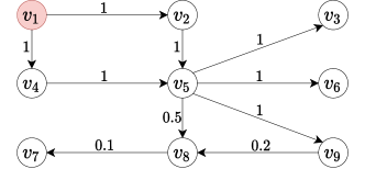
Figure 1: A toy graph $G$, where $v_{1}$ is the seed node and the value on each edge indicates its propagation probability.

Example 1.

Figure 1 shows a graph $G=(V,E)$ where $S=\{v_{1}\}$ is the seed set, and the value on each edge is its propagation probability, e.g., $p_{v_{5},v_{8}}=0.5$ indicates $v_{8}$ can be activated by $v_{5}$ with $0.5$ probability if $v_{5}$ becomes active. At timestamp $0$, seed $v_{1}$ node is activated while other nodes are inactive. At timestamps $1$ to $3$, the seed $v_{1}$ will certainly activate $v_{2},v_{3},v_{4},v_{5},v_{6}$ and $v_{9}$, as the corresponding activation probability is $1$. Because $v_{8}$ may be activated by either $v_{5}$ or $v_{9}$, we have $\mathcal{P}^{G}(v_{8},\{v_{1}\})=1-(1-p_{v_{5},v_{8}}\cdot\mathcal{P}^{G}(v_{5},\{v_{1}\}))(1-p_{v_{9},v_{8}}\cdot\mathcal{P}^{G}(v_{9},\{v_{1}\}))=1-0.5\times 0.8=0.6$. If $v_{8}$ is activated, it has $0.1$ probability to activate $v_{7}$. Thus, we have $\mathcal{P}^{G}(v_{7},\{v_{1}\})=p_{v_{8},v_{7}}\cdot\mathcal{P}^{G}(v_{8},\{v_{1}\})=0.6\times 0.1=0.06$. The expected spread is the activation probability sum of all the nodes, i.e., $\mathbb{E}(\{v_{1}\},G)=7.66$.

In IMIN problem, if we block $v_{5}$, the new expected spread $\mathbb{E}(\{v_{1}\},G[V\setminus\{v_{5}\}])=3$. Similarly, we have $\mathbb{E}(\{v_{1}\},G[V\setminus\{v_{2}\}])=\mathbb{E}(\{v_{1}\},G[V\setminus\{v_{4}\}])=6.66$, and blocking any other node also achieves a smaller expected spread than blocking $v_{5}$. Thus, if $b=1$, the result of the IMIN problem is $\{v_{5}\}$.

For IMIN-EB problem, if we block $(v_{5},v_{9})$, the expected spread will become $\mathbb{E}(\{v_{1}\},G(V,E\setminus\{(v_{5},v_{9})\}))=6.55$. Similarly, we have $\mathbb{E}(\{v_{1}\},G(V,E\setminus\{(v_{5},v_{3})\}))=6.66$, and blocking any other edge also achieves a smaller expected spread than blocking $(v_{5},v_{9})$. Thus, if the budget $b=1$, the result of the IMIN-EB problem is $\{(v_{5},v_{9})\}$.

3.3 Problem Hardness Analysis

To the best of our knowledge, no existing work has studied the hardness of the IMIN problem and IMIN-EB problem, as surveyed in Zareie and Sakellariou (2021). Thus, we need to analyze the problem hardness. For the approximation of the problem, in Section 5.2, we will present and prove that it is APX-hard for both two problems under the IC model, and our proposed greedy algorithms can achieve a $(1-1/e-\varepsilon)$-approximation for both two problems under the LT model.

Theorem 1.

Given a graph $G$, a seed set $S$ and a budget $b$, the IMIN problem is NP-Hard.

Proof Sketch. We reduce the densest k-subgraph (DKS) problem (Bhaskara et al. 2010), which is NP-hard, to the IMIN problem. For an arbitrary instance of the DKS problem, we can construct a corresponding instance of the IMIN problem, where the optimal blocker set in this instance corresponds to the optimal solution of the instance in the DKS problem. The fact that the DKS problem is unsolvable in PTIMES (polynomial time) implies that the IMIN problem is also unsolvable in PTIMES. Hence, the IMIN problem is proven to be NP-hard. The proof details can be found in the online appendix 1. $\square$

Theorem 2.

Given a graph $G$, a seed set $S$ and a budget $b$, the IMIN-EB problem is NP-Hard.

Proof Sketch. We reduce the IMIN problem to the IMIN-EB problem to prove the IMIN-EB problem is NP-hard. The proof details can be found in the online appendix 1. $\square$

3.4 A Baseline Algorithm

In this subsection, we review and discuss the baseline greedy algorithm, which is the most advanced existing solution to IMIN and IMIN-EB problem (Budak et al. 2011, Wang et al. 2013, Pham et al. 2019, Yan et al. 2020, Zhu et al. 2020). The baseline algorithm serves as a benchmark for comparison with our proposed algorithms.

The baseline greedy algorithm is as follows (psuedo-code in online appendix 2): we start with an empty blocker set (resp. edge set) $B=\varnothing$, and then iteratively add node $u$ (resp. edge $(u,v)$) into set $B$ that leads to the largest decrease of expected spread, i.e., $u=\arg\max_{u\in V\setminus(S\cup B)}(\mathbb{E}(S,G[V\setminus B])-\mathbb{E}(S,G[V\setminus(B\cup\{u\})]))$ (resp. $(u,v)=\arg\max_{(u,v)\in E\setminus B}(\mathbb{E}(S,G(V,E\setminus B))-\mathbb{E}(S,G(V,E\setminus(B\cup\{(u,v)\}))))$), until $|B|=b$.

As the greedy algorithms proposed by previous works use Monte-Carlo Simulations to compute the expected spread, each computation of spread decrease needs $O(r\cdot m)$ time, where $r$ is the number of rounds in Monte-Carlo Simulations. Thus, the time complexity of the baseline greedy algorithm is $O(b\cdot n\cdot r\cdot m)$ for the IMIN problem (resp. $O(b\cdot m\cdot r\cdot m)$ for the IMIN-EB problem).

As indicated by the complexity, the baseline greedy algorithm cannot efficiently handle the cases with large $b$. The greedy heuristic is usually effective on small $b$ values. However, it still incurs a significant time cost due to the need to enumerate the entire node set as candidate blockers and compute the expected spread for each candidate.

4 Computation of Decrease in Expected Spread

In this section, we propose an algorithm for efficiently estimating the reduction in expected spread resulting from blocking a single node in the graph. We first show that existing methods for calculating expected spread are not feasible for efficiently estimating the reduction in expected spread caused by each candidate blocker. (Section 4.1). Then, we propose a new framework (Section 4.4) that utilizes sampled graphs (Section 4.2) and their dominator trees (Section 4.3) to efficiently calculate the reduction in expected spread for each potential blocker. This computation can be performed with a single scan of the dominator trees. In addition, our approach can be utilized to estimate the reduction in the expected spread that arises from edge blocking by adding virtual nodes in the graph (Section 4.5).

From Multiple Seeds to One Seed. For presentation simplicity, we introduce the techniques for the case of one seed node. A unified seed node $s^{\prime}$ is created to replace all the seeds in the graph. For each node $u$, if there are $h$ different seeds pointing to $u$ and the probability on each edge is $p_{i}(1\leq i\leq h)$, we remove all the edges from the seeds to $u$ and add an edge from $s^{\prime}$ to $u$ with probability $(1-\prod_{i=1}^{h}(1-p_{i}))$ under the IC model (resp. $\sum_{i=1}^{h}p_{i}$ under the LT model).

4.1 Existing Works of Expected Spread Estimation

Previous research focuses on estimation algorithms for determining the expected influence spread, rather than exact computation. This is because computing the expected influence spread of a seed set in both IC and LT model is #P-hard (Chen et al. 2010), and the exact solution can only be used in small graphs (e.g., with a few hundred edges) (Maehara et al. 2017). There are two different existing methods for estimating the expected spread

Monte-Carlo Simulations (MCS). Kempe et al. (2003) apply MCS to estimate the influence spread, which is often used in some influence-related problems (e.g., Ishihata and Sato 2011, Ohsaka et al. 2014, Zhang et al. 2014). In each round of MCS: (a) for the IC model, it removes every edge $(u,v)$ with $(1-p_{u,v})$ probability; (b) for the LT model, for each node $v$, assume it has $k$ incoming edges $(u_{1},v),\cdots,(u_{k},v)$, $v$ has $p_{u_{i},v}(i\in[1,k])$ probability to have a unit incoming edge $(u_{i},v)$ and $1-\sum_{i=1}^{k}p_{u_{i},v}$ probability to have no incoming edge. Let $G^{\prime}$ be the resulting graph, and the set $R(s)$ contains the nodes in $G^{\prime}$ that are reachable from $s$ (i.e., there exists at least one path from $s$ to each node in $R(s)$). For the original graph $G$ and seed $s$, the expected size of set $R(s)$ equals the expected spread $\mathbb{E}(\{s\},G)$ (Kempe et al. 2003). Assuming we take $r$ rounds of MCS to estimate the expected spread, MCS needs $O(r\cdot m)$ times to calculate the expected spread. Recall that the IMIN (resp. IMIN-EB) problem is to find the optimal node (resp. edge) set with a given seed set. The spread computation by MCS for the two problems is costly. This is because the dynamic of influence spread caused by different nodes (resp. edges) is not fully utilized in the sampling. Consequently, it becomes necessary to repeatedly perform MCS for each candidate set.

Reverse Influence Sampling (RIS).  Borgs et al. (2014) propose the RIS to approximately estimate the influence spread, which is often used in the solutions for influence maximization (IMAX) problem (e.g., Sun et al. 2018, Guo et al. 2020). For each round, RIS generates an instance of $g$ randomly sampled from graph $G$ in the same way as MCS. Then a node $x$ is randomly sampled in $g$. It performs reverse breadth-first search (BFS) to compute the reverse reachable (RR) set of the node $x$, i.e., the nodes that can be reached by node $x$ in the reverse graph of $g$. They prove that if the RR set of node $v$ has $\rho$ probability to contain the node $u$ when $u$ is the seed node, we have $\rho$ probability to activate $v$. In the IMAX problem, RIS generates RR sets by sampling the nodes in the sampled graphs and then applying the greedy heuristic. As the expected influence spread is submodular of seed set $S$ (Kempe et al. 2005), an approximation ratio can be guaranteed by RIS in the IMAX problem. However, for the influence minimization problem, reversing the graph is not helpful. This is because the blockers (resp. edges which are blocked) appear to act as “intermediaries” between the seeds and other nodes. As a result, the computation cannot be unified into a single process in the reversing.

4.2 Expected Spread Estimation via Sampled Graphs

We first introduce the randomly sampled graph under the IC and LT models.

IC model. Let $\mathcal{G}$ be the distribution of the graphs with each induced by the randomness in edge removals from $G$, i.e., removing each edge $e=(u,v)$ in $G$ with $1-p_{u,v}$ probability. A random sampled graph $g$ derived from $G$ is an instance randomly sampled from $\mathcal{G}$.

LT model. Let $\mathcal{G}$ be the distribution of the graphs with each induced by the randomness in incoming edge selections from $G$, i.e., for each node $v$, assume it has $k$ incoming edges $(u_{1},v),\cdots,(u_{k},v)$, $v$ has $p_{u_{i},v}(i\in[1,k])$ probability to have a unit incoming edge $(u_{i},v)$ and $1-\sum_{i=1}^{k}p_{u_{i},v}$ probability to have no incoming edge. A random sampled graph $g$ derived from $G$ is an instance randomly sampled from $\mathcal{G}$. We summarize the notations related to the randomly sampled graph in Table A2.

The following lemma is a useful interpretation of expected spread (Maehara et al. 2017).

Lemma 1.

Suppose that the graph $g$ is a randomly sampled graph derived from $G$. Let $s$ be a seed node, we have $\mathbb{E}[\sigma(s,g)]=\mathbb{E}(\{s\},G)$.

By Lemma 1, we have the following corollary for computing the expected spread when blocking one node.

Corollary 1.

Given two fixed nodes $s$ and $u$ with $s\neq u$, and a random sampled graph $g$ derived from $G$, we have $\mathbb{E}[\sigma(s,g)-\sigma^{\rightarrow u}(s,g)]=\mathbb{E}(\{s\},G[V\setminus\{u\}])$.

Based on Lemma 1 and Corollary 1, we can compute the decrease of expected spread when a node is blocked.

Theorem 3.

Let $s$ be a fixed node, $u$ be a blocked node, and $g$ be a randomly sampled graph derived from $G$, respectively. For any node $u\in V(G)\setminus\{s\}$, we have the decrease of expected spread by blocking $u$ is equal to $\mathbb{E}[\sigma^{\rightarrow u}(s,g)]$, where $\mathbb{E}[\sigma^{\rightarrow u}(s,g)]=\mathbb{E}(\{s\},G)-\mathbb{E}(\{s\},G[V\setminus\{u\}])$.

As we use random sampling for estimating the decrease of the expected spread of each node, we show that the average number of $\sigma^{\rightarrow u}(s,g)$ is an accurate estimator of any node $u$ and fixed seed node $s$, when the number of sampled graphs is sufficiently large. Let $\theta$ be the number of sampled graphs, $\xi^{\rightarrow u}(s,G)$ be the average number of $\sigma^{\rightarrow u}(s,g)$ and $OPT$ be the exact decrease of expected spread from blocking node $u$, i.e., $OPT=\mathbb{E}[\sigma^{\rightarrow u}(s,g)]$ (Theorem 3). We use the Chernoff bounds (Motwani and Raghavan 1995) for theoretical analysis.

Lemma 2.

Let $X$ be the sum of $c$ i.i.d. random variables sampled from a distribution on $[0,1]$ with a mean $\mu$. For any $\delta>0$, we have $Pr[X-c\mu\geq\delta\cdot c\mu]\leq e^{-\delta^{2}c\mu/(2+\delta)}$ and $Pr[X-c\mu\leq-\delta\cdot c\mu]\leq e^{-\delta^{2}c\mu/2}.$

Theorem 4.

For seed node $s$ and a fixed node $u$, the inequality $|\xi^{\rightarrow u}(s,G)-OPT|<\varepsilon\cdot OPT$ holds with at least $1-{n^{-l}}$ probability when $\theta\geq\frac{l(2+\varepsilon)n\log n}{\varepsilon^{2}\cdot OPT}$.

4.3 Dominator Trees of Sampled Graphs

In order to efficiently compute the decrease in expected spread resulting from the blocking of individual nodes, we consider constructing the dominator tree (Aho and Ullman 1973) for each sampled graph. For the sampled graphs under the LT model, we can find that each node contains at most one incoming edge in each sampled graph, thus we first propose a linear algorithm for constructing dominator trees (Section 4.3.1). For the general graph, we apply the Lengauer-Tarjan algorithm (Lengauer and Tarjan 1979) to construct the dominator tree (Section 4.3.2).

Note that, in the following subsection, the id of each node is reassigned by the sequence of a depth-first search (DFS) on the graph starting from the seed.

Definition 5 (dominator).

Given $G=(V,E)$ and a source $s$, the node $u$ is a dominator of node $v$ when every path in $G$ from $s$ to $v$ has to go through $u$.

Definition 6 (immediate dominator).

Given $G=(V,E)$ and a source $s$, the node $u$ is the immediate dominator of node $v$, denoted $idom(v)=u$, if $u$ dominates $v$ and every other dominator of $v$ dominates $u$.

We can find that every node except source $s$ has a unique immediate dominator. The dominator tree of graph $G$ is induced by the edge set $\{(idom(u),u)\mid u\in V\setminus\{s\}\}$ with root $s$ (Lowry and Medlock 1969, Aho and Ullman 1973).

4.3.1 Dominator Tree Construction under the LT Model

We can find that each node in the sampled graphs under the LT model has at most one incoming edge. Thus, for each node in the sampled graphs, its immediate dominator is its unit in-neighbor.

Algorithm 1 illustrates the structure of a dominator tree under the LT model. It can be implemented in $O(m)$ time. We apply a breadth-first-search beginning from the seed (Lines 1-2). In each round, we use the front element in the queue (Line 4) to augment its out-neighbors for constructing the dominator tree (Lines 3-10).

Input : a sampled graph under the LT model $G$, and the source $s$

Output : $DT$ dominator tree of graph $G$

Push $s$ to the end of the queue $Q$;AlgoLine0.1

$vis\leftarrow\{s\},DT\leftarrow\varnothing$;AlgoLine0.2

while $Q$ is not empty do  $v\leftarrow$ the front element in $Q$, then pop the front element from $Q$; AlgoLine0.3

for each $u\in N^{out}_{v}$ do  if $u\not\in vis$ then  $vis\leftarrow vis\cup\{u\}$; AlgoLine0.4

Push $u$ to the end of the queue $Q$;AlgoLine0.5

add edge $(v,u)$ into $DT$;AlgoLine0.6

      return $DT$;AlgoLine0.7

Algorithm 1 DTC-LT($G,s$)

7

7

7

7

7

7

7

4.3.2 The Lengauer-Tarjan Algorithm

The Lengauer-Tarjan algorithm is an efficient algorithm for constructing the dominator tree. It first computes the semidominator of each node $u$, denoted by $sdom(u)$, where $sdom(u)=\min\{v\mid\text{there is a path~{}}v=v_{0},v_{1},\cdots,v_{k}=u\text{~{}with~{}}v_{i}>u\text{~{}for any integer~{}}i\in[1,k)\}$. The semi-dominator can be computed by finding the minimum $sdom$ value on the paths of the depth-first-search. The core idea of the Lengauer-Tarjan algorithm is to quickly compute the immediate dominators by the semi-dominators based on the following lemma. The details of the algorithm can be found in Lengauer and Tarjan (1979).

Lemma 3.

Lengauer and Tarjan (1979) Given $G=(V,E)$ and a source $s$, let $u\neq s$ and $v$ be the node with the minimum $sdom(v)$ among the nodes in the paths from $sdom(u)$ to $u$ (including $u$ but excluding $sdom(u)$), then we have $idom(u)=\left\{\begin{matrix}sdom(u)&\text{if }sdom(u)=sdom(v),\\ idom(v)&\text{otherwise}.\end{matrix}\right.$

The time complexity of the Lengauer-Tarjan algorithm is $O(m\cdot\alpha(m,n))$ which is almost linear, where $\alpha$ is the inverse function of Ackerman’s function (Ackermann 1928).

4.4 DESC Algorithm

Following the above subsections, if node $u$ is blocked, we can use the number of nodes in the subtree rooted at $u$ in the dominator tree to estimate the decrease in expected spread. Thus, using DFS on dominator trees, we can estimate the decrease of expected spread for blocked nodes.

Theorem 5.

Let $s$ be a fixed node in graph $g$. For any node $u\in(V(g)\setminus\{s\})$, we have $\sigma^{\rightarrow u}(s,g)$ equals to the size of the subtree rooted at $u$ in the dominator tree of graph $g$.

Thus, for each blocker $u$, we can estimate the decrease of the expected spread by the average size of the subtrees rooted at $u$ in the dominator trees of the sampled graphs.

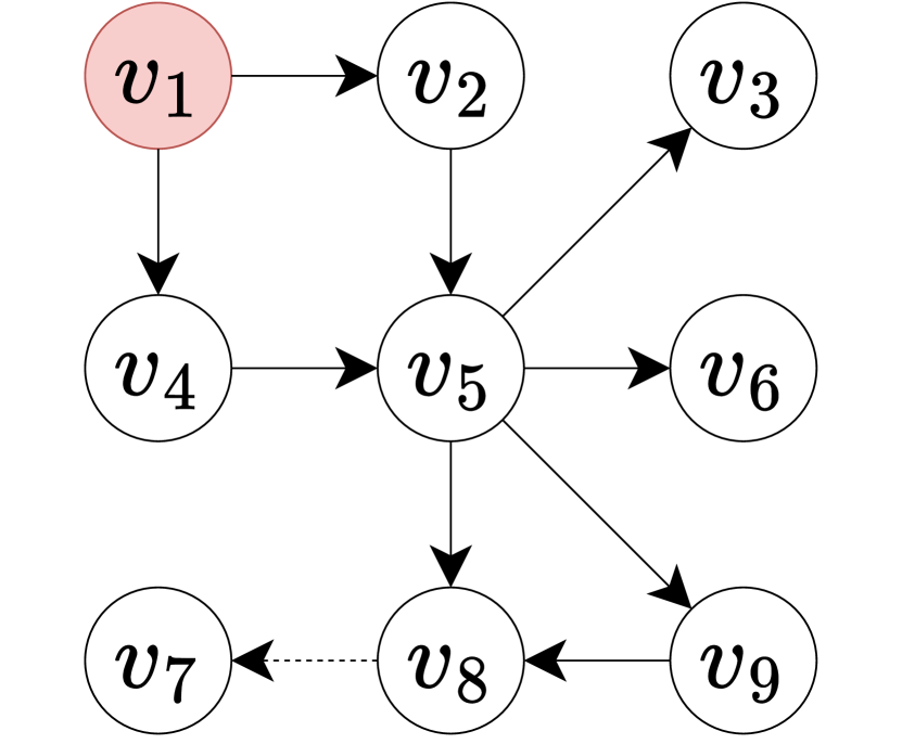
(a) Sampled Graph 1

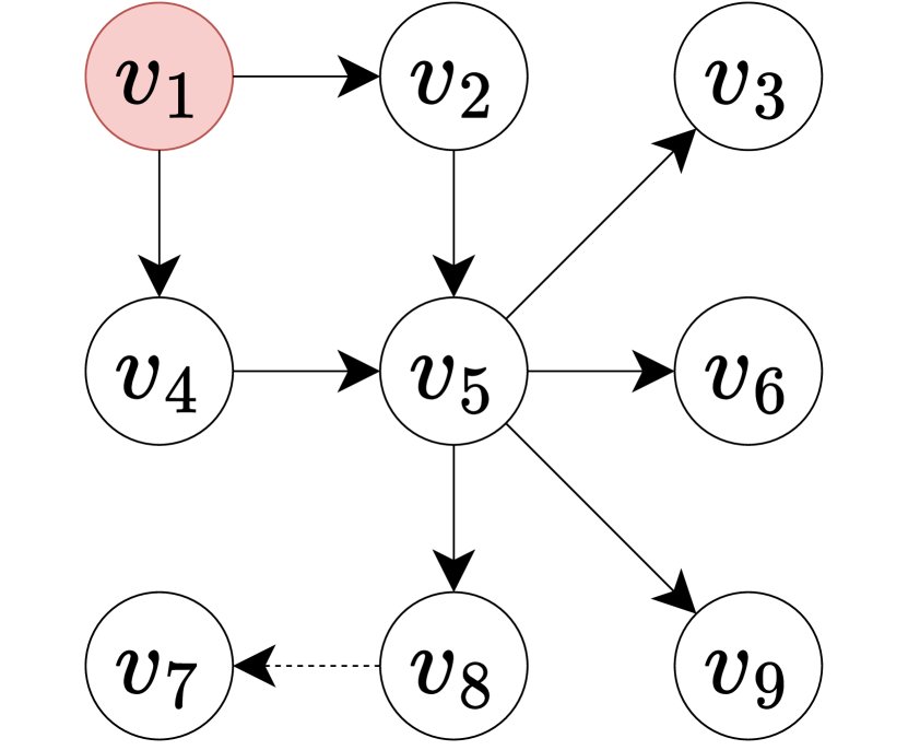
(b) Sampled Graph 2

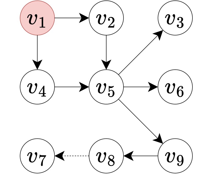
(c) Sampled Graph 3

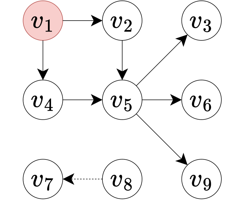
(d) Sampled Graph 4

Figure 2: Sampled graphs of the graph $G$ in Figure 1.

(a) DT of Graph in Fig. 2(a)

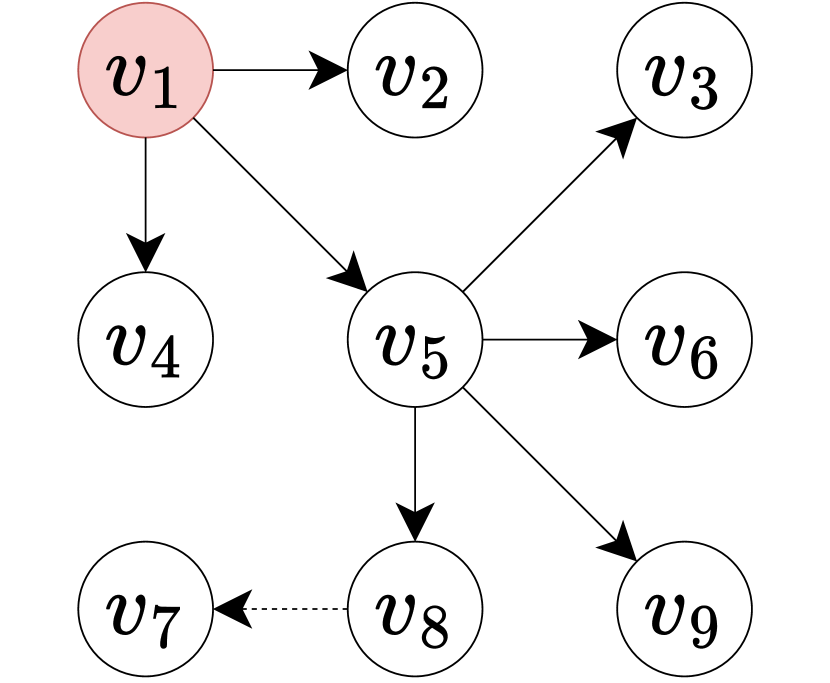
(b) DT of Graph in Fig. 2(b)

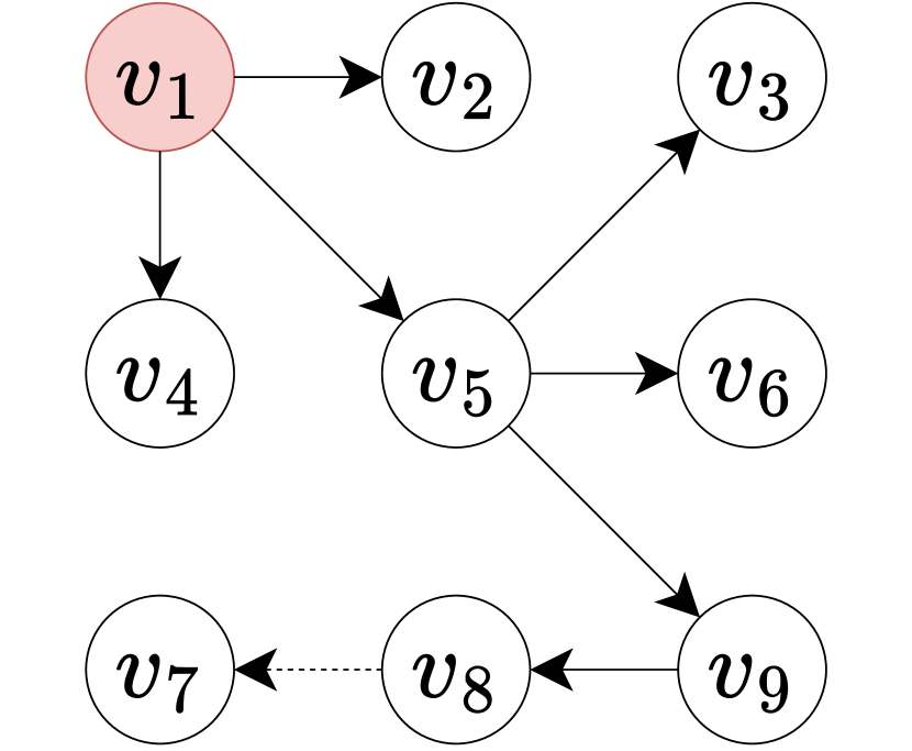
(c) DT of Graph in Fig. 2(c)

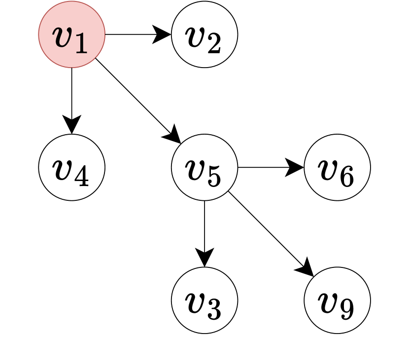
(d) DT of Graph in Fig. 2(d)

Figure 3: Dominator trees of the sampled graphs in Figure 2.

Example 2.

Considering the graph $G$ in Figure 1, there are only three edges with propagation probabilities less than $1$ (i.e., $(v_{5},v_{8})$, $(v_{9},v_{8})$ and $(v_{8},v_{7})$), and the other edges will exist in any sampled graph. Figures 2(a)-2(d) depict all the possible sampled graphs. For conciseness, we use the dotted edge $(v_{8},v_{7})$ to represent whether it may exist in a sampled graph or not (corresponding to two different sampled graphs, respectively). When $(v_{8},v_{7})$ is not in the sampled graphs, as $p_{v_{5},v_{8}}=0.5$ and $p_{v_{9},v_{8}}=0.2$, Figures 2(a), 2(b), 2(c) and 2(d) have $0.1,0.4,0.1$ and $0.4$ to exist, respectively. As $p_{v_{8},v_{7}}=0.1$, $v_{1}$ can reach $8+0.1=8.1$ nodes in expectation in Figure 2(a). Similarly, $v_{1}$ can reach $8.1,8.1$ and $7$ nodes (including $v_{1}$) in expectation in Figures 2(b), 2(c) and 2(d), respectively. Thus, the expected spread of graph $G$ is $7.66$, which is the same as the result we compute in Example 1.

Figures 3(a)-3(d) show the corresponding dominator trees of the sampled graphs in Figure 2. For node $v_{5}$, the expected sizes of the subtrees rooted at $v_{5}$ are $5.1,5.1,5.1$ and $4$ in the dominator trees, respectively. Thus, the blocking of $v_{5}$ will lead to a $4.66$ decrease in the expected spread. As the sizes of subtrees of $v_{2},v_{3},v_{4}$, and $v_{6}$ are only $1$ in each dominator tree, blocking any of them will lead to a $1$ expected spread decrease. Similarly, blocking $v_{7}$, $v_{8}$ and $v_{9}$ will lead to $0.66$, $0.06$ and $1.11$ expected spread decrease, respectively.

Input : a graph $G$, the source $s$ and the number of sampled graphs $\theta$

Output : $\Delta[u]$ for each $u\in V(G)\setminus\{s\}$, i.e., the decrease of expected spread when $u$ is blocked

$\Delta[\cdot]\leftarrow 0$;AlgoLine0.1

for $i\leftarrow 1$ to $\theta$ do  Generate a sampled graph $g$ derived from $G$; AlgoLine0.2

$DT\leftarrow$ dominator tree of $g$ (Algorithm 1 or Lengauer-Tarjan algorithm (Section 4.3.2));AlgoLine0.3

$c[\cdot]\leftarrow$ the size of subtree in tree $DT$ when each node is the root;AlgoLine0.4

$\Delta[u]\leftarrow\Delta[u]+c[u]/\theta$ for each $u\in V(g)\setminus\{s\}$;AlgoLine0.5

  AlgoLine0.6

return $\Delta[\cdot]$

Algorithm 2 DESC($G,s,\theta$)

6

6

6

6

6

6

We propose the DESC algorithm for computing the decrease of the expected spread of each node, Algorithm 2 shows the details. We set $\Delta[\cdot]$ as $0$ initially (Line 1). Then we generate $\theta$ different sampled graphs derived from $G$ (Lines 2-3). For each sampled graph, we first construct the dominator tree through Algorithm 1 or Lengauer-Tarjan (Line 4). Then we use a simple DFS to compute the size of each subtree. After computing the average size of the subtrees and recording it in $\Delta[\cdot]$ (Line 6), we return $\Delta[\cdot]$ (Line 7). As computing the sizes of the subtrees through DFS costs $O(m)$, Algorithm 2 runs in $O(\theta\cdot m\cdot\alpha(m,n))$ under the IC model (resp. $O(\theta\cdot m)$ under the LT model).

4.5 Decrease in Expected Spread from Blocking Edge

For the IMIN-EB problem, we further need to estimate the decrease of expected spread when each edge is blocked in the graph. We first construct edge-sampled graphs, denoted by $g^{E}$, based on graph $G$. Let $g$ be a sampled graph based on graph $G$. For each edge $(u,v)\in E(g)$, we use a virtual node $w_{u,v}$ to represent this edge. The edge-sampled graph $g^{E}$ contains two parts: $V_{V}$ and $V_{E}$. $V_{V}$ contains $n$ nodes where each node corresponds to $v\in V(g)$. $V_{E}$ contains $m$ nodes, i.e., $V_{E}=\cup_{(u,v)\in E(g)}w_{u,v}$. We then add edges $(u,w_{u,v})$ and $(w_{u,v},v)$ in the graph $g^{E}$ for each edge $(u,v)\in E(g)$. We can compute the decrease of expected spread led by edge $(u,v)$ through node $w_{u,v}$ on edge-sampled graphs.

Theorem 6.

Let $s$ be a fixed node and $g^{E}$ be a random edge-sampled graph derived from $G$. Let $R_{u,v}$ be a set of nodes satisfying: (i) in the part $V_{V}$; (ii) reachable from $s$ in $g^{E}$ and (iii) all paths from $s$ in $g^{E}$ pass through $w_{u,v}$. For any edge $(u,v)$, we have the decrease of expected spread by blocking $(u,v)$ is equal to $\mathbb{E}[|R_{u,v}|]$.

We then present how to compute the node set $R_{u,v}$ for each node $w_{u,v}$ in $V_{E}$.

Theorem 7.

Let $s$ be a fixed node in graph $G$. We construct a dominator tree of edge-sampled graph $g^{E}$ based on graph $G$. For any node $w_{u,v}\in V_{E}$, we have $R_{u,v}$ are the nodes in $V_{V}$ and the subtree rooted at $w_{u,v}$ in the dominator tree of graph $g^{E}$.

Input : a graph $G$, the source $s$ and the number of sampled graphs $\theta$

Output : $\Delta[u,v]$, i.e., the decrease of expected spread when $(u,v)$ is blocked

$\Delta[\cdot]\leftarrow 0$;AlgoLine0.1

for $i\leftarrow 1$ to $\theta$ do  Generate a sampled graph $g$ derived from $G$; AlgoLine0.2

$V_{V}\leftarrow V(g)$;AlgoLine0.3

Generate a edge-sampled graph $g^{E}$ based on $g$;AlgoLine0.4

Construct a dominator tree $DT$ of graph $g^{E}$;AlgoLine0.5

$R[\cdot]\leftarrow V_{V}\cap$ the nodes in subtree in tree $DT$ when each node is the root;AlgoLine0.6

$\Delta[u,v]\leftarrow\Delta[u,v]+|R[u,v]|/\theta$ for each $w_{u,v}\in V(g^{E})\setminus V_{V}$;AlgoLine0.7

  AlgoLine0.8

return $\Delta[\cdot]$

Algorithm 3 DESCE($G,s,\theta$)

8

8

8

8

8

8

8

8

Based on Theorem 6 and 7, we propose the DESCE algorithm (Algorithm 3) for computing the decrease of the expected spread of each edge. We set $\Delta[\cdot]$ as $0$ initially (Line 1). Then we generate $\theta$ different edge-sampled graphs derived from $G$ (Lines 2-5). For each sampled graph, we first construct the dominator tree through Algorithm 1 or Lengauer-Tarjan (Line 6). Then we can use a DFS to compute the size of $R_{u,v}$ from leaves to root (Line 7). After computing the average size of the $R_{u,v}$ and recording it in $\Delta[\cdot]$ (Line 8), we return $\Delta[\cdot]$ (Line 9).

As computing the sizes of the $R_{u,v}$ through DFS costs $O(m)$, Algorithm 3 runs in $O(\theta\cdot m\cdot\alpha(m,n))$ under the IC model (resp. $O(\theta\cdot m)$ under the LT model).

5 Our Proposed Algorithms

In this section, applying the new framework of expected spread estimation for selecting the candidates (Algorithm 2), we propose our AdvancedGreedy algorithm (Section 5.1) with higher efficiency and without sacrificing the effectiveness, compared with the baseline. We then prove our AdvancedGreedy algorithm can achieve a $(1-1/e-\varepsilon)$-approximation under the LT model. However, under the IC model, the problems are APX-hard (Section 5.2). As the greedy approaches do not consider the cooperation of candidate blockers during the selection, some important nodes may be missed, e.g., some out-neighbors of the seed. Thus, we further propose a superior heuristic, the GreedyReplace algorithm, to achieve a better result quality under the IC model (Section 5.3).

5.1 The AdvancedGreedy Algorithm

Based on Section 3.4 and Section 4.4, we propose the AdvancedGreedy algorithm with high efficiency. In the greedy algorithm, we aim to greedily find the node $u$ (resp. edge $(u,v)$) that leads to the largest decrease in the expected spread. Algorithm 2 and 3 can efficiently compute the expected spread decrease of every candidate node/edge. Thus, we can directly choose the node/edge which can cause the maximum decrease of expected spread to block.

Input : a graph $G$, seed $s$, budget $b$, the number of sampled graphs $\theta$, and candidate node/edge set $CB$

Output : the blocked node/edge set $B$

$B\leftarrow$ empty;AlgoLine0.1

for $i\leftarrow 1$ to $b$ do  $\Delta[\cdot]\leftarrow$ DESC($G[V\setminus B],s,\theta$) or DESCE($G[V\setminus B],s,\theta$); AlgoLine0.2

$B\leftarrow B\cup\{x\}$, where $x=\operatorname*{arg\,max}_{c\in CB}\Delta[c]$;AlgoLine0.3

  return $B$

Algorithm 4 AdvancedGreedy($G,s,b,\theta,CB$)

3

3

3

Algorithm 4 presents the pseudo-code of our AdvancedGreedy algorithm. For the IMIN-EB problem, we cannot block all nodes in the sampled graph (i.e., can block $V_{E}$ in the edge-sampled graph $g^{E}$), thus we need a candidate blocker set $CB$ as the input of the algorithm. For IMIN problem, $CB=V(G)\setminus\{s\}$, but for IMIN-EB problem, $CB=V_{E}=\cup_{(u,v)\in E(G)}w_{u,v}$. We start with the empty blocker set (Line 1). In each of the $b$ iterations (Line 2), we first estimate the decrease of the expected spread of each node (Line 3), find the node $x$ such that $\Delta[x]$ is the largest as the blocker and insert it to blocker set (Line 4). Finally, the algorithm returns the blocker set $B$ (Line 5).

Comparison with Baseline Algorithm. One round of MCS on $G$ will generate a graph $G^{\prime}$ where $V(G^{\prime})=V(G)$ and each edge in $E(G)$ will appear in $G^{\prime}$ if the simulation picks this edge. Thus, if we have $r=\theta$, our computation based on sampled graphs will not sacrifice the effectiveness, compared with MCS. For efficiency, Algorithm 4 runs in $O(b\cdot\theta\cdot m\cdot\alpha(m,n))$ for both two problems and the time complexity of the baseline (Algorithm 6) are $O(b\cdot r\cdot m\cdot n)$ and $O(b\cdot r\cdot m\cdot m)$. As $\alpha(m,n)$ is much smaller than $n$ and $m$, our AdvancedGreedy algorithm has a lower time complexity without sacrificing the effectiveness, compared with the baseline algorithm.

5.2 Approximation Guarantee of the AdvancedGreedy Algorithm

In this subsection, we discuss the approximation guarantee of the AdvancedGreedy algorithm under IC and LT models. For the IMIN problem, we first prove the function of the expected spread is monotone and not supermodular under the IC model.

Theorem 8.

Given a graph $G$ and a seed set $S$, the expected spread function $\mathbb{E}(S,G[V\setminus B])$ is monotone and not supermodular of $B$ under the IC model.

We then prove that the IMIN problem under the IC model is APX-hard.

Theorem 9.

Under the IC model, the IMIN problem is APX-hard unless P=NP.

However, we find that the function of expected spread is both monotone and supermodular under the LT model in the IMIN problem.

Theorem 10.

Given a graph $G$ and a seed set $S$, the expected spread function $\mathbb{E}(S,G[V\setminus B])$ is monotone and supermodular of $B$ under the LT model.

As the expected spread is non-increasing and supermodular of blocker set $B$ (Theorem 10), the AdvancedGreedy algorithm gives a $(1-1/e-\varepsilon)$-approximation to the optimum for IMIN problem under the LT model (Tzoumas et al. 2016).

We then analyze the function of the expected spread in the IMIN-EB problem.

Theorem 11.

Given a graph $G$ and a seed set $S$, the expected spread function $\mathbb{E}(S,G(V,E\setminus B))$ is monotone and not supermodular of $B$ under the IC model.

Theorem 12.

Given a graph $G$ and a seed set $S$, the expected spread function $\mathbb{E}(S,G(V,E\setminus B))$ is monotone and supermodular of $B$ under the LT model.

Therefore, as the expected spread is non-increasing and supermodular of blocked edge set $B$ (Theorem 12), the AdvancedGreedy algorithm gives a $(1-1/e-\varepsilon)$-approximation to the optimum for IMIN-EB problem under the LT model (Tzoumas et al. 2016).

Similar to Theorem 2, we can prove the IMIN-EB problem is APX-hard unless P=NP by reducing the IMIN problem to IMIN-EB problem based on Theorem 9.

Theorem 13.

Under the IC model, the IMIN-EB problem is APX-hard unless P=NP.

5.3 The GreedyReplace Algorithm

As the greedy algorithm does not achieve an approximate guarantee under the IC model, we further propose the GreedyReplace algorithm to improve its effectiveness.

We can find that some out-neighbors of the seed may be an essential part of the result while they may be missed by current greedy heuristics. Thus, we propose a new heuristic (GreedyReplace) which is to first select $b$ out-neighbors of the seed as the initial blockers, and then greedily replace a blocker with another node if the expected spread will decrease.

Example 3.

Considering the graph in Figure 1 with the seed $v_{1}$. When $b=1$, Greedy chooses $v_{5}$ as the blocker because it leads to the largest expected spread decrease ($v_{3},v_{6},v_{7},v_{8}$, and $v_{9}$ will not be influenced by $v_{1}$, i.e., the expected spread is $3$). When $b=2$, it further blocks $v_{2}$ or $v_{4}$ in the second round, and the expected spread becomes $2$. OutNeighbors only considers blocking $v_{2}$ and $v_{4}$. It blocks either of them when $b=1$ ($\mathbb{E}(\cdot)=6.66$), and blocks both of them when $b=2$ ($\mathbb{E}(\cdot)=1$).

In this example, we find that the performance of the Greedy algorithm is better than the OutNeighbors when $b$ is small, but its expected spread may become larger than OutNeighbors with the increase of $b$. As the budget $b$ can be either small or large in different applications, it is essential to further improve the heuristic algorithm.

Due to the above motivation, we propose the GreedyReplace algorithm as a solution to address the defects of the Greedy and OutNeighbors algorithms, while also combining their advantages. We first greedily choose $b$ out-neighbors of the seed as the initial blockers. Then, we replace the blockers according to the reverse order of the out-neighbors’ blocking order. As we can use Algorithm 2 to compute the decrease of the expected spread of blocking any other node, in each round of replacement, we set all the nodes in $V(G)\setminus(\{s\}\cup B)$ as the candidates for replacement. We will early terminate the replacement procedure when the node to replace is the current best blocker.

The expected spread of GreedyReplace is certainly not larger than the algorithm which only blocks the out-neighbors. Through the trade-off between choosing the out-neighbors and the replacement, the cooperation of the blockers is considered in GreedyReplace.

Example 4.

Considering the graph in Figure 1 with the seed $v_{1}$. When $b=1$, GreedyReplace first considers the out-neighbors as the candidate blockers and sets $v_{2}$ or $v_{4}$ as the blocker. As blocking $v_{5}$ can achieve a smaller influence spread than both $v_{2}$ and $v_{4}$, it will replace the blocker with $v_{5}$, thus the expected spread is $3$. When $b=2$, GreedyReplace first block $v_{2}$ and $v_{4}$, and there is no better node to replace. The expected spread is $1$. GreedyReplace achieves the best performance for either $b=1$ or $b=2$, compared to the Greedy and OutNeighbors algorithms.

Input : a graph $G$, the source $s$, budget $b$ and the number of sampled graphs $\theta$

Output : the blocker set $B$

$CB\leftarrow N^{out}_{s}$; $B\leftarrow$ empty;AlgoLine0.1

for $i\leftarrow 1$ to $\min\{d^{out}_{s},b\}$ do  $\Delta[\cdot]\leftarrow$ DESC($G[V\setminus B],s,\theta$); AlgoLine0.2

$x\leftarrow\operatorname*{arg\,max}_{u\in CB}\Delta[u]$; $CB\leftarrow CB\setminus\{x\}$; $B\leftarrow B\cup\{x\}$;AlgoLine0.3

  AlgoLine0.4

for each $u\in B$ with the reversing order of insertion do  $B\leftarrow B\setminus\{u\}$; $\Delta[\cdot]\leftarrow$ DESC($G[V\setminus B],s,\theta$); AlgoLine0.5

$x\leftarrow\operatorname*{arg\,max}_{u\in V(G)\setminus B}\Delta[u]$; $B\leftarrow B\cup\{x\}$;AlgoLine0.6

if $u=x$ then Break;AlgoLine0.7

  return $B$

Algorithm 5 GreedyReplace($G,s,b,\theta$)

7

7

7

7

7

7

7

Algorithm 5 shows the pseudo-code of GreedyReplace. We first push all out-neighbors of the seed into candidate blocker set $CB$ and set blocker set empty initially (Line 1). For each round, we choose the candidate blocker which leads to the largest expected spread decrease as the blocker, and then update $CB$ and $B$ (Lines 3-4). Then we consider replacing the blockers in $B$ by the reversing order of their insertions (Line 5). We remove the replaced node from the blocker set and use Algorithm 2 to compute the decrease of expected spread $\Delta[\cdot]$ for each candidate blocker (Line 6). We use $x$ to record the node with the largest spread decrease computed so far, by enumerating each of the candidate blockers (Line 7). If the node to replace is the current best blocker, we will early terminate the replacement (Line 8). Algorithm 5 returns the set $B$ of $b$ blockers (Line 9).

The time complexity of GreedyReplace is $O(\min\{d^{out}_{s},b\}\cdot\theta\cdot m\cdot\alpha(m,n))$. As the time complexity of Algorithm 2 is mainly decided by the number of edges in the sampled graphs, in practice the time cost is much less than the worst case.

6 Experiments

In this section, extensive experiments are conducted to validate the effectiveness and efficiency of our proposed algorithms.

6.1 Experimental Setting

Datasets. The experiments are conducted on $8$ real-world datasets, obtained from SNAP. Table 1 shows the statistics of the datasets, ordered by the number of edges in each dataset, where $d_{avg}$ is the average node degree (the sum of in-degree and out-degree for each directed graph) and $d_{max}$ is the largest node degree. For an undirected graph, we consider each edge as bi-directional. These experiments cover a diverse range of networks, spanning from networks consisting of 1,000 nodes and 25,000 edges to networks comprising 1 million nodes and 3 million edges.

Propagation Models. Our algorithm is designed for the IC and LT models with nonuniform propagation probabilities $p_{u,v}$ for each directed edge $(u,v)$. To generate these nonuniform probabilities $p_{u,v}$, we employ two propagation models following the existing literature.

1. Trivalency (TR) model (Jung et al. 2012, Chen et al. 2010, Yan et al. 2020): The propagation probability $p_{u,v}$ for each edge $(u,v)$ is randomly chosen from the set {0.1, 0.01, 0.001}, which correspond to high, medium, and low influences, respectively.

2. Weighted cascade (WC) model (Kempe et al. 2003, Tang et al. 2014): The propagation probability $p_{u,v}$ for each edge $(u,v)$ is $1/d^{in}_{v}$, where $d^{in}_{v}$ is the in-degree of $v$.

Table 1: Statistics of Datasets

Dataset	Abbr.	Description	Node	Edge $(u,v)$	$n$	$m$	$d_{avg}$	$d_{max}$	Type
EmailCore	EC	email data	member	$u$ sent at least one email to $v$	1,005	25,571	49.6	544	Directed
Facebook	F	social network	user	$u$ and $v$ are friends	4,039	88,234	43.7	1,045	Undirected
Wiki-Vote	W	vote data	user	$u$ voted on user $v$	7,115	103,689	29.1	1,167	Directed
EmailAll	EA	email data	user	$u$ sent at least one email to $v$	265,214	420,045	3.2	7,636	Directed
DBLP	D	bibliography	author	$u$ and $v$ are co-authors	317,080	1,049,866	6.6	343	Undirected
Twitter	T	social network	user	$u$ and $v$ are friends	81,306	1,768,149	59.5	10,336	Directed
Stanford	S	website pages	page	$u$ has hyperlinks to $v$	281,903	2,312,497	16.4	38,626	Directed
Youtube	Y	social network	user	$u$ and $v$ are friends	1,134,890	2,987,624	5.3	28,754	Undirected

Settings. Unless otherwise specified, we set $r=10^{4}$ for MCS , and for our sampled-graph-based algorithms (AdvancedGreedy and GreedyReplace), we sample $10^{4}$ graphs in the experiments. In each of our experiments, we independently execute each algorithm 5 times and report the average result. By default, we terminate an algorithm if the running time reaches 24 hours. Based on the results of the $\theta$ selection study (details in the online appendix 4), we set $\theta=10^{4}$ for all experiments.

Environments. The experiments are performed on a CentOS Linux serve (Release 7.5.1804) with Quad-Core Intel Xeon CPU (E5-2640 v4 @ 2.20GHz) and 128G memory. All the algorithms are implemented in C++. The source code is compiled by GCC(7.3.0) under O3 optimization.

Algorithms. The experiments involve comparing our proposed algorithms, namely the GreedyReplace and AdvancedGreedy, with both the greedy algorithms and other basic heuristics mentioned in the existing literature. The algorithms evaluated in our experiments are listed below.

1. Exact : This algorithm identifies the optimal solution by searching all possible combinations of $b$ blockers and uses MCS with $r=10^{4}$ to compute the expected spread of each candidate set of blockers. The algorithms demonstrate optimal effectiveness without considering efficiency, providing a benchmark for effectiveness comparison.

2. Rand (RA): This algorithm randomly chooses $b$ blockers (excluding the seeds) in the graph.

3. OutDegree (OD) (Rita et al. 2000, Newman et al. 2002): This algorithm selects $b$ nodes with the highest out-degrees as the blockers for the IMIN problem and selects $b$ directed edges where the ending nodes have the highest out-degrees for IMIN-EB problem.

4. BaselineGreedy (BG)  (Budak et al. 2011, Wang et al. 2013, Yan et al. 2020): This algorithm represents the current state-of-the-art approach. We have introduced and discussed in detail in Section 3.4. It leverages the MCS technique to estimate the expected spread.

5. AdvancedGreedy (AG): Our proposed AdvancedGreedy algorithm (Algorithm 4), which applies dominator tree techniques for estimating the reduction of expected spread.

6. GreedyReplace (GR): Our proposed GreedyReplace algorithm (Algorithm 5). It enhances the AdvancedGreedy algorithm by considering the relationships among candidate blockers.

6.2 Effectiveness Comparison

In this section, we first evaluate our proposed algorithms in comparison to the Exact algorithm, which represent the maximum achievable effectiveness without considering efficiency. Subsequently, we evaluate the efficacy of our proposed algorithms in comparison to other existing heuristics documented in the literature.

Comparison with the Exact Algorithm. As AG has an approximate guarantee under the LT model in both IMIN problem and IMIN-EB problem, we only compare the result of GR with the Exact algorithm under the IC model in two problems. Due to the huge time cost of Exact, we extract small datasets by iteratively extracting a node and all its neighbors, until the number of extracted nodes reaches $100$ in IMIN problem (resp. edges reaches $100$ in IMIN-EB problem). For EmailCore, we extract $5$ such subgraphs. We randomly choose $10$ nodes as the seeds. As the graph is small, we can use the exact computation of the expected spread (Maehara et al. 2017) for comparison between Exact and GR. We demonstrate that the expected spread of the GR algorithm closely aligns with the results of the Exact algorithm in both the TR Model (Tables 2 Panel A and Panel B) and the WC Model (Table A3 Panel C and Panel D in online appendix). Additionally, the GR algorithm outperforms the Exact algorithm in terms of speed, with a difference of up to six orders of magnitude in both the IMIN problem and the IMIN-EB problem. The results indicate that our proposed algorithms are highly effective and can achieve optimal results in a shorter timeframe.

Table 2: Exact v.s. GreedyReplace (IC model)

b	Expected Spread			Running Time (s)		Expected Spread			Running Time (s)
	Exact	GR	Ratio	Exact	GR	Exact	GR	Ratio	Exact	GR
	Panel A: IMIN Problem (TR Model)					Panel B: IMIN-EB Problem (TR Model)
1	12.614	12.614	100%	3.07	0.12	10.873	10.873	100%	3.04	0.10
2	12.328	12.334	99.95%	130.91	0.21	10.652	10.655	99.9%	150.72	0.31
3	12.112	12.119	99.94%	3828.2	0.25	10.454	10.459	99.9%	5373.9	0.35
4	11.889	11.903	99.88%	80050	0.33	10.360	10.407	99.5%	90897	0.40

Table 3: Expected Spread in the IMIN problem (IC model)

b	EmailCore (TR model)				Facebook (TR model)				Wiki-Vote (TR model)				EmailAll (TR model)
	RA	OD	AG	GR	RA	OD	AG	GR	RA	OD	AG	GR	RA	OD	AG	GR
20	354.88	230.10	220.59	219.69	16.059	16.026	11.717	11.691	512.62	325.51	131.30	130.77	548.99	286.05	14.642	13.640
40	341.33	98.712	84.022	83.823	16.037	16.019	10.416	10.413	512.18	222.00	46.747	43.898	546.94	221.97	10.319	10.002
60	325.13	47.249	35.085	33.634	16.033	16.010	10.151	10.149	507.11	138.60	25.514	23.282	546.39	148.52	10	10
80	304.90	30.277	19.001	18.848	15.997	15.987	10.028	10.026	501.49	32.646	17.332	17.322	545.41	100.84	10	10
100	283.54	22.696	13.640	13.533	15.994	15.980	10.001	10.001	496.05	25.831	14.726	14.518	544.59	55.398	10	10
b	DBLP (TR model)				Twitter (TR model)				Stanford (TR model)				Youtube (TR model)
	RA	OD	AG	GR	RA	OD	AG	GR	RA	OD	AG	GR	RA	OD	AG	GR
20	13.747	13.730	10.502	10.499	16801	16610	16101	16100	16.087	16.075	12.069	10.483	14.774	14.762	14.743	10.950
40	13.739	13.725	10.079	10.079	16796	16470	15749	15748	16.080	16.071	10.488	10.234	14.773	14.755	10.075	10.002
60	13.737	13.721	10.012	10.010	16786	16329	15447	14972	16.071	16.040	10.136	10.075	14.773	14.750	10	10
80	13.720	13.714	10	10	16780	16175	14610	14474	16.064	16.017	10.026	10.019	14.767	14.742	10	10
100	13.716	13.706	10	10	16771	16057	13619	13181	16.052	15.989	10.009	10.002	14.762	14.729	10	10

Table 4: Expected Spread in the IMIN-EB problem (IC model)

b	EmailCore (TR model)				Facebook (TR model)				Wiki-Vote (TR model)				EmailAll (TR model)
	RA	OD	AG	GR	RA	OD	AG	GR	RA	OD	AG	GR	RA	OD	AG	GR
20	364.62	364.42	361.54	361.51	57.846	58.04	33.346	33.279	484.60	487.94	167.93	166.79	1,567.0	1566.2	361.51	338.46
40	364.53	364.36	357.15	356.48	57.829	57.829	23.748	23.702	481.22	482.27	42.768	40.205	1,561.9	1564.1	83.462	81.488
60	364.42	364.23	336.62	333.41	57.669	57.579	18.901	18.859	480.61	482.20	17.329	16.311	1,556.6	1561.0	28.143	23.414
80	364.30	364.10	281.97	267.79	57.568	57.363	15.624	15.611	479.28	475.20	11.491	11.360	1,556.6	1558.2	14.049	12.954
100	364.12	363.81	206.65	189.50	57.322	57.316	13.330	13.329	475.67	472.55	10.101	10.086	1,551.9	1550.7	11.783	11.590
b	DBLP (TR model)				Twitter (TR model)				Stanford (TR model)				Youtube (TR model)
	RA	OD	AG	GR	RA	OD	AG	GR	RA	OD	AG	GR	RA	OD	AG	GR
20	10.690	10.692	10.451	10.354	16,800	16,800	16,701	16697	13.477	13.456	11.540	10.989	10.819	10.817	10.081	10.069
40	10.686	10.688	10.253	10.144	16,800	16,799	16,760	16607	13.471	13.439	10.512	10.487	10.803	10.817	10.031	10.025
60	10.684	10.687	10.055	10.037	16,799	16,799	16,588	16567	13.503	13.460	10.232	10.105	10.801	10.814	10.006	10.005
80	10.682	10.685	10.023	10.015	16,799	16,797	16,552	15650	13.469	13.555	10.097	10.011	10.800	10.804	10.002	10.001
100	10.673	10.669	10.016	10.004	16,796	16,797	16486	11479	13.518	13.453	10.040	10	10.797	10.790	10	10

Comparison with Other Heuristics. As discussed in Section 5.1, the effectiveness (expected spread) of the AG algorithm is the same as the BG algorithm. Thus, we compare the effectiveness (i.e., expected spread) of our proposed algorithms (AG and GR) with other heuristics (RA and OD) on all networks (EC, F, W, EA, D, T, S, Y) under the IC model in Tables 3 (IMIN problem) and Table 4 (IMIN-EB problem). The results under the LT model are included in the Tables A6 and A7 in online appendix. We first randomly select $10$ nodes as the seeds and vary the budget $b$ from $20,40,60,80$ to $100$. We repeat this process by $5$ times and report the average expected spread with the resulting blockers (the expected spread is computed by MCS with $10^{5}$ rounds). The bold numbers in Table 3 and 4 denote the minimum expected spread across the four algorithms. The results under the WC model can be found in Table A4 and Table A5 in the online appendix.

The findings indicate that our GR algorithm consistently attains the optimal outcome, characterized by the lowest expected spread, across various budgets and in both propagation models. The performance of the GR algorithm surpasses that of the other algorithms. Moreover, as the budget $b$ increases, the efficacy of the GR algorithm improves. The findings substantiate the superiority of our proposed algorithm, GR, in terms of effectiveness when compared to other existing algorithms.

6.3 Efficiency Comparison

In this section, we first compare the efficiency of our proposed algorithms (AG and GR) with state-of-the-art BG algorithms. Then, we demonstrate the scalability of our proposed GR algorithm.

Time Cost of Different Algorithms. We compare the running time of BG, AG, and GR, and set the budget $b$ to $10$ due to the huge computation cost of the BG. Figures 4 and 5 show the results for all networks under the two propagation models where the x-axis denotes different networks and the y-axis is the running times (s) of the algorithms. For the IMIN problem, the BG algorithm is unable to return results within the specified time constraint of 24 hours for six networks under the TR model, and for five networks under the WC model. For IMIN-EB problem, the BG algorithm does not return any results within 72 hours in all datasets, while the number of candidates of IMIN-EB is much larger than IMIN (the number of edges v.s. the number of nodes). The results indicate that our proposed algorithms, namely AG and GR algorithms, exhibit significantly better runtime performance compared to existing state-of-the-art BG algorithm. The difference in runtime is at least three orders of magnitude, and this gap tends to be even larger when applied to larger networks. These results align with the analysis of time complexities presented in Section 5.1. Additionally, the time required for GR is similar to that of AG. We can also observe that the running time of all three algorithms under the LT model is generally smaller than under the IC model. This is likely due to the fact that the sampled graphs in the LT model are smaller, as each node can have at most one in-neighbor. Additionally, the speedup in running time for the AG and GR algorithms is greater compared to the BG, which can be attributed to the strict linear refinement of these two algorithms under the LT model.

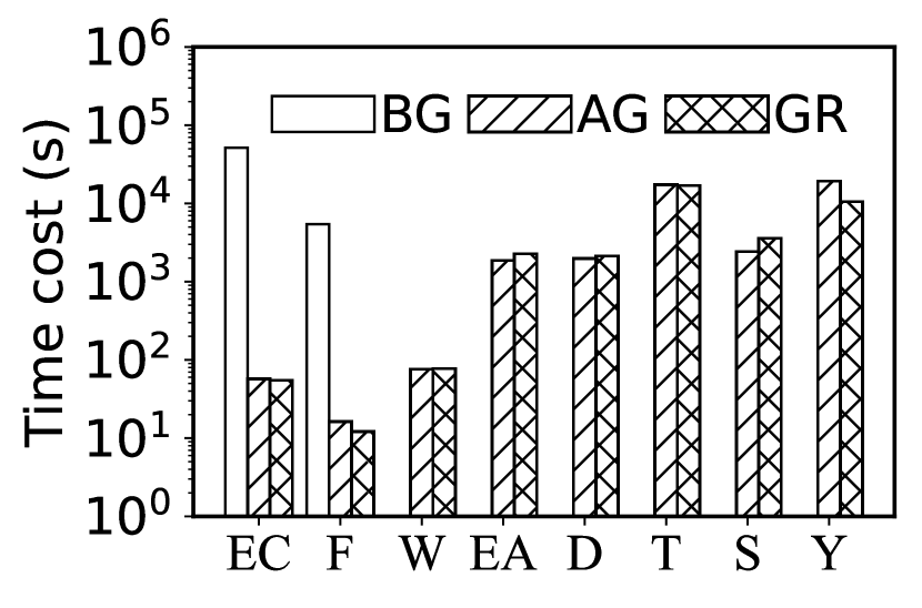
(a) TR & IC model

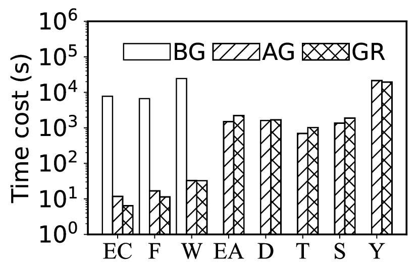
(b) WC & IC model

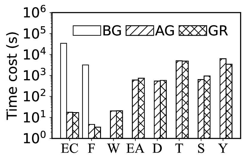
(c) TR & LT model

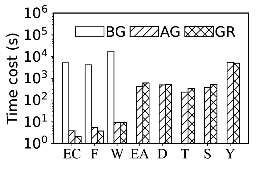
(d) WC & LT model

Figure 4: Time Cost of Different Algorithms in the IMIN problem

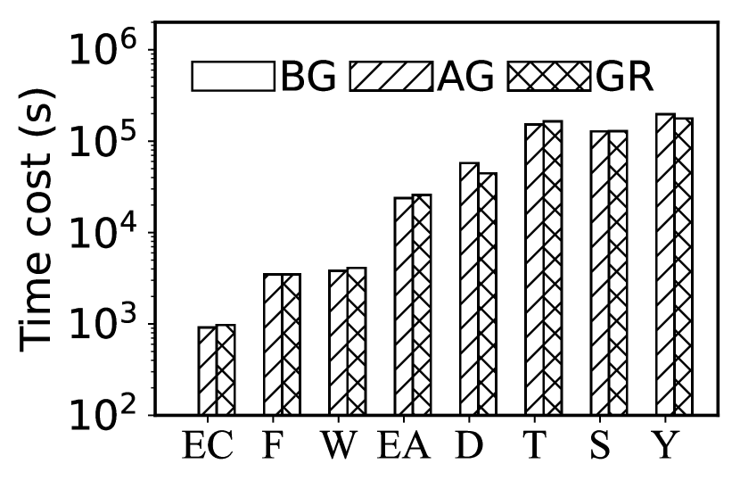
(a) TR & IC model

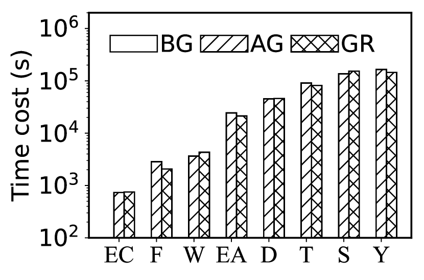
(b) WC & IC model

(c) TR & LT model

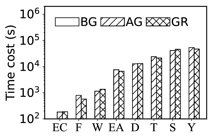
(d) WC & LT model

Figure 5: Time Cost of Different Algorithms in the IMIN-EB problem

Varying the Budget. The running time of the algorithms on Facebook and DBLP networks is shown in Figure 6 for various budgets. The running time of AG may decrease with larger budgets due to the early termination implemented in Algorithm 5 (Lines 19-20). It is evident that our proposed algorithms AG and GR exhibit significantly greater efficiency in comparison to the most advanced existing method BG, with the disparity between them further enlarged as the budget expands. Additionally, it is observed that the computational time required for AG is similar to that of GR. AG may exhibit faster performance than GR in cases where the budget is limited. However, as the budget increases, GR demonstrates superior performance in terms of running time.

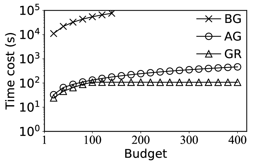
(a) Facebook (TR model)

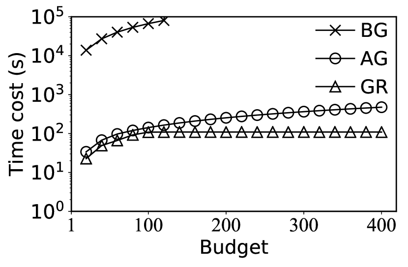
(b) Facebook (WC model)

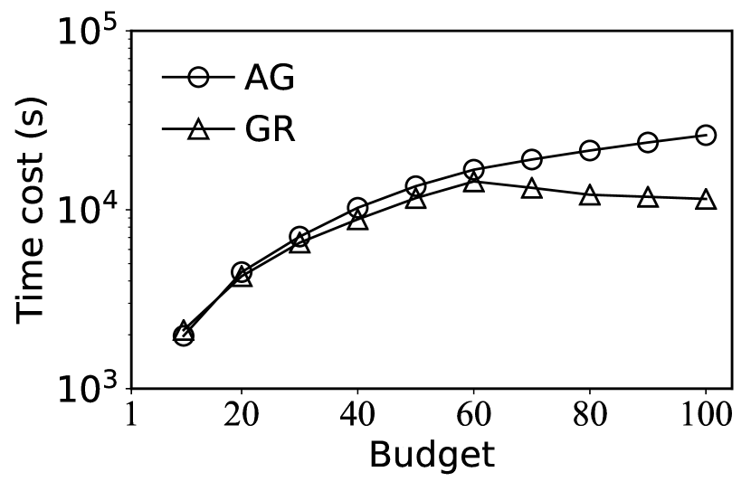
(c) DBLP (TR model)

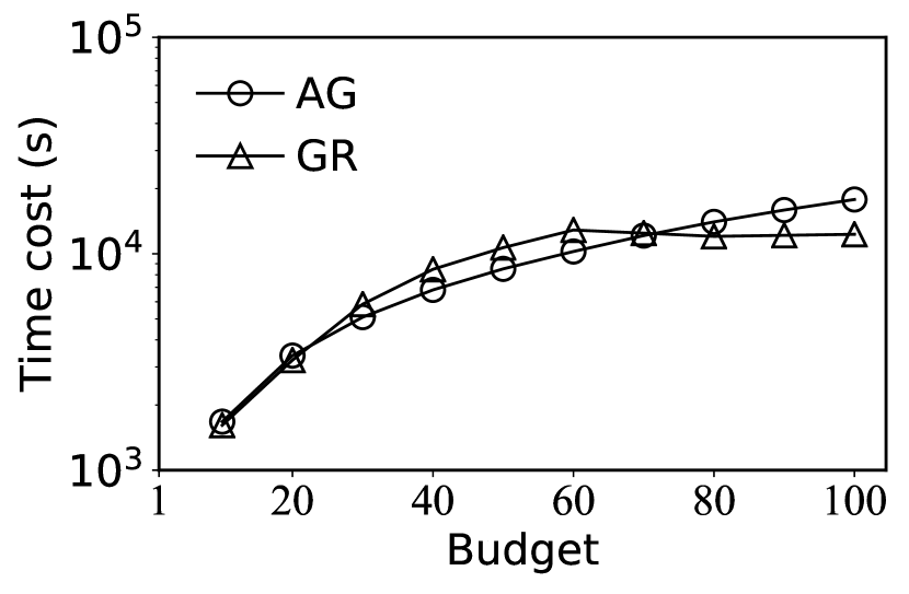
(d) DBLP (WC model)

Figure 6: Running Time v.s. Budget in the IMIN problem (IC model)

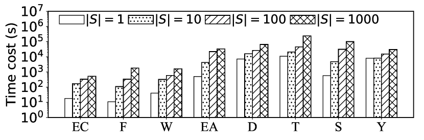
(a) TR Model

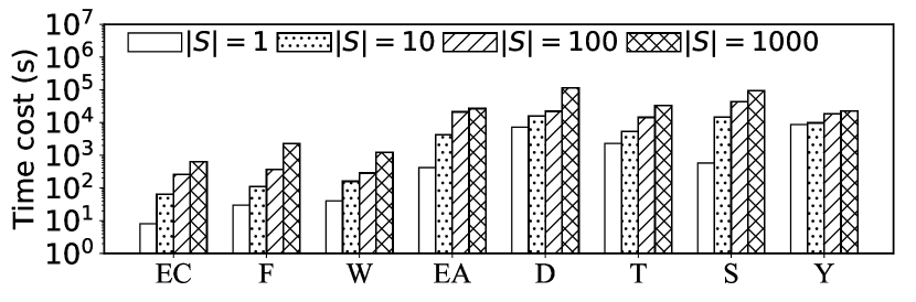
(b) WC Model

Figure 7: Running Time v.s. Number of Seeds (IMIN problem under the IC model)

Scalability. The scalability of our GR algorithm is assessed in Figure 7(a) and Figure 7(b). We set the budget to $100$ and vary the number of seeds from $1,10,100$ to $1000$. We report the average time cost of the GR algorithm by executing it 5 times. We can see that as the number of seeds increases, so does the running duration. This is due to the fact that a greater number of seeds results in a greater influence spread (a larger size of sampled graphs), and the running duration of Algorithm 2 is highly correlated with the size of sampled graphs. We can also observe that the proportional increase in running time is much less than the proportional increase in the number of seeds, proving that GR is scalable enough to manage scenarios with a large number of seeds.

7 Conclusion

This study focuses on the influence minimization problem, specifically the selection of a blocker set consisting of $b$ nodes or $b$ edges to minimize the influence spread from a given seed set. This problem is critical yet relatively understudied, with the potential to tackle urgent societal challenges such as combating misinformation spreads and managing epidemic outbreaks. A major obstacle in influence minimization has been the absence of efficient and scalable techniques suitable for handling large networks. Existing approaches often struggle with the computational burden posed by real-life large networks, which hinders their practicality and effectiveness. Through meticulous analysis, we have successfully proven the NP-hardness of the influence minimization problem. Additionally, this study introduces the AdvancedGreedy algorithm as a novel approach to enhance the efficiency of existing algorithms while maintaining their effectiveness, surpassing them by a remarkable three orders of magnitude. The efficiency of our algorithm is enhanced by simultaneously computing the reduction in expected influence spread using sampled graphs and their dominator trees. Furthermore, we introduce the GreedyReplace algorithm as an enhancement to the greedy method. This algorithm incorporates a new heuristic, resulting in improved effectiveness. Our proposed AdvancedGreedy and GreedyReplace algorithms have been extensively tested on $8$ real-life datasets, and the results confirm their superior performance compared to other existing algorithms in the literature. In summary, our proposed algorithm’s unprecedented speedup marks a turning point in the feasibility of influence minimization, which empowers timely decision-making in scenarios where rapid intervention is paramount.

Despite the contributions of our paper, it is important to discuss the limitations and future directions of our research. First, this study assumes a static network, but the algorithms proposed here can serve as inspiration for developing efficient and effective algorithms for dynamic networks. Additionally, future research can explore efficient parallel and distributed solutions based on the proposed algorithms. Furthermore, it would be worthwhile to investigate more efficient heuristics that provide satisfactory trade-offs in terms of result quality.

Online Appendix 1: Proofs

Proof of Theorem 1

Proof.

We reduce the densest k-subgraph (DKS) problem (Bhaskara et al. 2010), which is NP-hard, to the IMIN problem. Given an undirected graph $G(V,E)$ with $|V|=n$ and $|E|=m$, and an positive integer $k$, the DKS problem is to find a subset $A\subseteq V$ with exactly $k$ nodes such that the number of edges induced by $A$ is maximized.

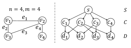
Figure A1: Construction example for hardness proofs, where the left part of the figure is an instance of DKS problem and the right part is its corresponding construction of IMIN problem.

Consider an arbitrary instance $G(V=\{v_{1},\cdots,v_{n}\},E=\{e_{1},\cdots,e_{m}\})$ of DKS problem with a positive integer $k$, we construct a corresponding instance of IMIN problem on graph $G^{\prime}$. Figure A1 shows a construction example from $4$ nodes and $4$ edges.

The graph $G^{\prime}$ contains three parts: $C$, $D$, and a seed node $S$. The part $C$ contains $n$ nodes, i.e., $C=\cup_{1\leq i\leq n}c_{i}$ where each $c_{i}$ corresponds to $v_{i}$ of instance $G$. The part $D$ contains $m$ nodes, i.e., $D=\cup_{1\leq i\leq m}d_{i}$ where each node $d_{i}$ corresponds to edge $e_{i}$ in instance $G$. The node $S$ is the only seed of the graph. For each edge $e_{i}=(v_{x},v_{y})$ in graph $G$, we add two edges: (i) from $c_{x}$ to $d_{i}$ and (ii) $c_{y}$ to $d_{i}$. Then we add an edge from $S$ to each $c_{i}(1\leq i\leq n)$. The propagation probability of each edge is set to $1$. The construction of $G^{\prime}$ is completed.

We then show the equivalence between the two instances. As the propagation probability of each edge is $1$, the expected spread in the graph is equal to the number of nodes that can be reached by seed $S$. Adding a node $v_{i}$ into node set $A$ corresponds to the removal of $c_{i}$ from the graph $G^{\prime}$, i.e., $c_{i}$ is blocked. If edge $e_{i}$ is in the induced subgraph, the corresponding node $d_{i}$ in $G^{\prime}$ cannot be reached by seed $S$. We find that blocking the nodes $c_{i}\in C$ will first lead to the decrease of expected spread of themselves, and the nodes in $D$ may also not be reached by $S$ if both two in-neighbors of them are blocked. Thus, blocking the corresponding nodes $c_{i}$ of $v_{i}\in A$ will lead to $|A|+g$ decrease of expected spread, where $g$ is the number of nodes in $D$ that cannot be reached by $S$ (equals to the number of edges in the induced subgraph $G[A]$). Note that there is no need to block nodes in $D$, because they do not have any out-neighbors, and blocking them only leads to the decrease of expected spread of themselves which is not larger than the decrease of the expected spread of blocking the nodes in $C$. We can find that IMIN problem will always block $k$ nodes, as blocking one node will lead to at least $1$ decrease of expected spread.

The optimal blocker set $B$ of IMIN problem corresponds to the optimal node set $A$ of DKS problem, where each node $c_{i}\in B$ corresponds to the set $v_{i}\in A$. Thus, if the IMIN problem can be solved in PTIME, the DKS problem can also be solved in PTIME, while the DKS problem is NP-hard. ∎

Proof of Theorem 2

Proof.

We reduce the IMIN problem to IMIN-EB problem. Consider an arbitrary instance $G(V=\{v_{1},\cdots,v_{n}\},E=\{e_{1},\cdots,e_{m}\})$ of IMIN problem with a positive integer $b$, we construct a corresponding instance of IMIN-EB problem on graph $G^{\prime}(V^{\prime},E^{\prime})$. There are $2n$ nodes in graph $G^{\prime}$, i.e., $V^{\prime}=\cup_{1\leq i\leq n}\{v_{i}^{in},v_{i}^{out}\}$ where each pair of nodes $\{v_{i}^{in},v_{i}^{out}\}$ corresponds to node $v_{i}$ in instance $G$. For each edge $e_{i}=(v_{x},v_{y})$ in graph $G$, we add edge from $v_{x}^{out}$ to $v_{y}^{in}$ in graph $G^{\prime}$. We further add edges from $v_{i}^{in}$ to $v_{i}^{out}$ for each pair $\{v_{i}^{in},v_{i}^{out}\}$ with probability $1$. We can find that the decrease of the expected spread led by $(v_{x}^{out},v_{y}^{in})$ is always less than or equal to $(v_{x}^{in},v_{x}^{out})$, thus we always block edges from $v_{x}^{in}$ to $v_{x}^{out}$, which is equal to block node $v_{x}$ in the IMIN problem. Thus the IMIN-EB problem can not be solved in PTIME. ∎

Proof of Corollary 1

Proof.

Let $g^{\prime}=g[V(g)\setminus\{u\}]$, we have $\sigma(s,g)-\sigma^{\rightarrow u}(s,g)=\sigma(s,g^{\prime})$. Thus, $\mathbb{E}[\sigma(s,g)-\sigma^{\rightarrow u}(s,g)]=\mathbb{E}[\sigma(s,g^{\prime})]$. As $g^{\prime}=g[V(g)\setminus\{u\}]$, $g^{\prime}$ can be regarded as a random sampled graph derived from graph $G[V\setminus\{u\}]$. By Lemma 1, $\mathbb{E}[\sigma(s,g^{\prime})]=\mathbb{E}(\{s\},G[V\setminus\{u\}])$. Therefore, $\mathbb{E}[\sigma(s,g)-\sigma^{\rightarrow u}(s,g)]=\mathbb{E}(\{s\},G[V\setminus\{u\}])$. ∎

Proof of Theorem 3

Proof.

As $\sigma^{\rightarrow u}(s,g)=\sigma(s,g)-(\sigma(s,g)-\sigma^{\rightarrow u}(s,g))$, we have $\mathbb{E}[\sigma^{\rightarrow u}(s,g)]=\mathbb{E}[\sigma(s,g)]-\mathbb{E}[\sigma(s,g)-\sigma^{\rightarrow u}(s,g)]$. From Corollary 1, we have $\mathbb{E}[\sigma(s,g)-\sigma^{\rightarrow u}(s,g)]=\mathbb{E}(\{s\},G[V\setminus\{u\}])$. By Lemma 1, we know $\mathbb{E}[\sigma(s,g)]=\mathbb{E}(\{s\},G)$. Therefore, $\mathbb{E}[\sigma^{\rightarrow u}(s,g)]=\mathbb{E}(\{s\},G)-\mathbb{E}(\{s\},G[V\setminus\{u\}])$. ∎

Proof of Theorem 4

Proof.

We have $Pr[|\xi^{\rightarrow u}(s,G)-OPT|\geq\varepsilon\cdot OPT]$ $\begin{matrix}=&Pr[|\frac{\xi^{\rightarrow u}(s,G)\cdot\theta}{n}-\frac{OPT\cdot\theta}{n}|\geq\frac{\varepsilon\cdot\theta}{n}\cdot OPT]\\ \end{matrix}$.

Let $\delta=\varepsilon$, $\mu=\frac{OPT}{n}$ and $X=\frac{\xi^{\rightarrow u}(s,G)\cdot\theta}{n}$. According to Lemma 2, we have $Pr[|\xi^{\rightarrow u}(s,G)-OPT|\geq\varepsilon\cdot OPT]$ $=Pr[|X-\theta\mu|\geq\delta\cdot\theta\mu]\leq exp(\frac{-\delta^{2}\theta\mu}{2+\delta})=exp(\frac{-\varepsilon^{2}\theta OPT}{n(2+\varepsilon)})$.

As $\theta\geq\frac{l(2+\varepsilon)n\log n}{\varepsilon^{2}\cdot OPT}$, we have $Pr[|\xi^{\rightarrow u}(s,G)-OPT|\geq\varepsilon\cdot OPT]\leq exp(l\log n)=n^{-l}$. Therefore, $|\xi^{\rightarrow u}(s,G)-OPT|<\varepsilon\cdot OPT$ holds with at least $1-n^{-l}$ probability. ∎

Proof of Theorem 5

Proof.

Let $c[u]$ denote the size of the subtree with root $u$ in the dominator tree of graph $g$. Assume $v$ is in the subtree with $u$ (i.e., $u$ is the ancestor of $v$), from the definition of dominator, we have $v$ cannot be reached by $s$ when $u$ is blocked. Thus, $c[u]\leq\sigma^{\rightarrow u}(s,g)$. If $v$ is not in the subtree, i.e., $u$ does not dominate $v$ in the graph, there is a path from $s$ to $v$ not through $u$, which means blocking $u$ will not affect the reachability from $s$ to $v$. We have $\sigma^{\rightarrow u}(s,g)=c[u]$. ∎

Proof of Theorem 6

Proof.

As only nodes in $G$ have activation probability, based on Lemma 1, the expected number of nodes in $V_{V}$ is equal to the expected spread of $G$. We can find that blocking the edge $(u,v)$ in graph $G$ will remove the node $w_{u,v}$ from graph $g^{E}$. From Theorem 3, we have the decrease of expected spread by blocking edge $(u,v)$ in $G$ is equal to the decrease of expected spread by blocking node $w_{u,v}$ in $g^{E}$, i.e., the expected number of nodes in $R_{u,v}$. ∎

Proof of Theorem 7

Proof.

From Theorem 5, we know nodes satisfying (a) reachable from $s$ in $g^{E}$ and (b) all the paths from $s$ in $g^{E}$ pass through $w_{u,v}$ constitute the subtree rooted at $w_{u,v}$. $R_{u,v}$ further requires nodes are in the $V_{V}$, and thus $R_{u,v}$ contains the nodes that both in $V_{V}$ and subtree rooted at $w_{u,v}$. ∎

Proof of Theorem 8

Proof.

As adding any blocker to any set $B$ cannot increase the expected influence spread, we have $\mathbb{E}(S,G[V\setminus B])$ is monotone of $B$. For every two set $X\subseteq Y\subseteq V$ and node $x\in V\setminus Y$, if function $f(\cdot)$ is supermodular, it must hold that $f(X\cup\{x\})-f(X)\leq f(Y\cup\{x\})-f(Y)$. Consider the graph in Figure 1, let $f(B)=\mathbb{E}(S,G[V\setminus B])$, $X=\{v_{3}\},Y=\{v_{2},v_{3}\}$ and $x=v_{4}$. As $f(X)=6.66$, $f(Y)=5.66$, $f(X\cup\{x\})=5.66$, and $f(Y\cup\{x\})=1$, we have $f(X\cup\{x\})-f(X)=-1>f(Y\cup\{x\})-f(Y)=-4.66$. ∎

Proof of Theorem 9

Proof.

We use the same reduction from the densest k-subgraph (DKS) problem to the Influence Minimization problem, as in the proof of Theorem 1. Densest k-subgraph (DKS) problem does not have any polynomial-time approximation scheme, unless P=NP (Khot 2006). According to the proof of Theorem 1, we have a blocker set $B$ for influence minimization problem on $G^{\prime}$ corresponding to a node set $A$ for DKS problem, where each $c_{i}\in B$ corresponds to $v_{i}\in A$. Let $x$ denote the number of edges in the optimal result of DKS, and $y$ denote the optimal spread in IMIN, we have $x+k=y$, where $k$ is the given positive number of DKS problem. If there is a solution with $\gamma$-approximation on the influence minimization problem, there will be a $\lambda$-approximation on the DKS problem. Thus, there is no PTAS for the influence minimization problem, and it is APX-hard unless P=NP. ∎

Proof of Theorem 10

Proof.

As adding any blocker to any set $B$ cannot increase the expected influence spread, we have $\mathbb{E}(S,G[V\setminus B])$ is monotone of $B$. In the sampled graphs under the LT model, we know that the immediate dominator of each node is its unit in-neighbor, thus the children in the dominator tree of each node are the nodes that are reachable from it. Therefore, blocking any node $u$ in the graph leads to remove the edge $(fa_{u},u)$ in the dominator tree, where $fa_{u}$ denotes the father node of node $u$ in the dominator tree. We can find that, for any node $u$ in each sampled graph, adding any blocker to any set $B$ cannot increase the number of nodes $u$. Let $f(B)=\mathbb{E}(S,G[V\setminus B])$, we have for any two set $X,Y(X\subseteq Y\subseteq V)$ and a node $u\in V$, $f(X)-f(X\cup\{u\})\geq f(Y)-f(Y\cup\{u\})$. ∎

Online Appendix 2: Baseline Algorithm Psuedo-code

Input : a graph $G$ and the source $s$

Output : the blocker (resp. edge) set $B$

$B\leftarrow$ empty;AlgoLine0.1

for $i\leftarrow 1$ to $b$ do  $x\leftarrow-1$; AlgoLine0.2

for each $u\in V(G)\setminus(B\cup\{s\})$ (resp. each $(u,v)\in E(G)\setminus B$) do  $\Delta\leftarrow$ decrease of expected spread when blocking $u$ (resp. $(u,v)$); AlgoLine0.3

if $x=-1$ or $\Delta>\Delta[x]$ then  $x\leftarrow u$ (resp. $x\leftarrow(u,v)$); AlgoLine0.4

    $B\leftarrow B\cup\{x\}$;AlgoLine0.5

  return $B$

Algorithm 6 BaselineGreedy($G,s$)

5

5

5

5

5

Online Appendix 3: Tables

Table A1: Summary of Notations

Notation	Definition
$G=(V,E)$	a directed graph with node set $V$ and edge set $E$
$n;m$	number of nodes/edges in $G$ (assume $m>n$)
$V(G);E(G)$	the set of nodes/edges in $G$
$G[V^{\prime}]$	the subgraph in $G$ induced by node set $V^{\prime}$
$N^{in}_{u};N^{out}_{u}$	the set of in-neighbors/out-neighbors of node $u$
$d^{in}_{u};d^{out}_{u}$	the in-degree/out-degree of node $u$
$S;s$	the seed set; a seed node
$B$	the blocker set
$\theta$	the number of sampled graphs used in algorithm
$Pr[x]$	the probability if $x$ is true
$\mathbb{E}[x]$	the expectation of variable $x$
$p_{u,v}$	the probability that node $u$ activates node $v$
$\mathcal{P}^{G}(x,S)$	the probability that node $x$ is activated by set $S$ in $G$
$\mathbb{E}(S,G)$	the expected influence spread, i.e., the expected number of activated non-seed nodes in graph $G$ from seed set $S$

Table A2: Notations for Random Sampled Graph

Notation	Definition
$\sigma(s,G)$	the number of nodes reachable from $s$ in $G$
$\sigma^{\rightarrow u}(s,G)$	the number of nodes reachable from $s$ in $G$, where all the paths from $s$ to these nodes pass through $u$
$\xi^{\rightarrow u}(s,G)$	the average number of $\sigma^{\rightarrow u}(s,G)$ in the sampled graphs which are derived from $G$

Table A3: Exact v.s. GreedyReplace (IC model)

b	Expected Spread			Running Time (s)		Expected Spread			Running Time (s)
	Exact	GR	Ratio	Exact	GR	Exact	GR	Ratio	Exact	GR
	Panel C: IMIN Problem (WC Model)					Panel D: IMIN-EB Problem (WC Model)
1	11.185	11.185	100%	2.63	0.10	11.882	11.882	100%	4.03	0.12
2	11.077	11.078	99.99%	110.92	0.18	11.634	11.697	99.5%	205.21	0.25
3	10.997	10.998	99.99%	3284.0	0.23	11.344	11.421	99.3%	7375.2	0.37
4	10.922	10.925	99.97%	69415	0.33	11.269	11.279	99.9%	98247	0.50

Table A4: Comparision with Other Heuristics (Expected Spread) in IMIN problem (IC model)

b	EmailCore (WC model)				Facebook (WC model)				Wiki-Vote (WC model)				EmailAll (WC model)
	RA	OD	AG	GR	RA	OD	AG	GR	RA	OD	AG	GR	RA	OD	AG	GR
20	82.605	54.907	53.516	53.296	21.482	21.362	14.588	14.554	24.102	22.660	17.765	17.701	13.330	11.493	10.720	10.455
40	75.990	44.710	40.199	40.093	21.456	21.360	12.425	12.418	23.971	21.696	15.258	15.222	13.234	11.447	10.111	10.086
60	69.947	37.561	31.891	31.784	21.429	21.297	11.194	11.187	23.899	20.409	13.749	13.743	13.217	11.408	10	10
80	64.154	32.580	26.094	26.073	21.417	21.176	10.476	10.474	23.763	12.798	12.654	12.574	13.188	11.385	10	10
100	57.170	24.959	21.926	21.899	21.395	21.056	10.013	10.012	23.757	12.711	12.138	12.129	13.070	11.324	10	10
b	DBLP (WC model)				Twitter (WC model)				Stanford (WC model)				Youtube (WC model)
	RA	OD	AG	GR	RA	OD	AG	GR	RA	OD	AG	GR	RA	OD	AG	GR
20	118.23	118.17	32.602	32.601	259.45	235.73	199.40	198.76	25.803	25.800	11.742	11.740	25.663	25.368	10.152	10.113
40	118.16	117.81	18.429	18.409	258.86	226.28	170.20	168.64	25.790	25.779	10.435	10.398	25.585	25.330	10.012	10.006
60	118.09	117.73	11.869	11.867	257.75	214.90	144.61	144.23	25.777	25.771	10.119	10.101	25.446	25.149	10	10
80	117.97	117.59	10	10	255.48	204.17	129.53	128.75	25.685	25.633	10.005	10.002	25.346	25.113	10	10
100	117.94	117.43	10	10	254.04	196.40	114.11	112.07	25.657	25.603	10.002	10.000	25.277	25.052	10	10

Table A5: Comparision with Other Heuristics (Expected Spread) in IMIN-EB problem (IC model)

b	EmailCore (WC model)				Facebook (WC model)				Wiki-Vote (WC model)				EmailAll (WC model)
	RA	OD	AG	GR	RA	OD	AG	GR	RA	OD	AG	GR	RA	OD	AG	GR
20	110.48	109.56	98.538	96.303	34.122	34.679	18.245	17.784	14.559	14.549	12.633	12.585	135.77	134.68	112.28	96.303
40	108.94	109.28	90.809	90.303	34.084	34.415	15.200	15.146	14.517	14.449	11.685	11.668	135.52	134.60	93.690	90.327
60	107.77	108.26	83.598	82.780	34.006	33.979	13.721	13.638	14.462	14.448	11.063	11.041	135.34	134.46	83.598	75.873
80	106.78	107.77	78.104	77.089	33.779	33.974	12.842	12.811	14.449	14.416	10.618	10.603	134.68	133.74	55.483	54.509
100	106.49	106.25	73.944	71.778	33.775	33.952	12.160	12.127	14.446	14.344	10.303	10.285	133.65	133.18	37.619	37.383
b	DBLP (WC model)				Twitter (WC model)				Stanford (WC model)				Youtube (WC model)
	RA	OD	AG	GR	RA	OD	AG	GR	RA	OD	AG	GR	RA	OD	AG	GR
20	12.943	12.957	11.915	11.531	182.89	181.91	165.14	164.77	30.707	30.503	16.758	16.717	36.406	36.428	26.471	25.339
40	12.932	12.948	10.963	10.834	181.96	180.82	157.06	155.303	30.572	30.495	14.427	14120	36.393	36.383	21.303	20.353
60	12.928	12.929	10.725	10.596	181.43	180.02	150.74	150.266	30.564	30.225	12.485	12.489	36.373	36.368	16.358	15.433
80	12.906	12.927	10.398	10.319	180.44	179.73	145.82	144.653	30.292	29.894	10.971	10.262	36.370	36.358	11.407	10.385
100	12.895	12.922	10.146	10.070	180.08	178.95	141.99	141.681	30.034	29.693	10.187	10.136	36.363	36.319	10	10

Table A6: Comparision with Other Heuristics (Expected Spread) in IMIN problem (LT model)

b	EmailCore (WC model)			Facebook (WC model)			Wiki-Vote (WC model)			EmailAll (WC model)
	RA	OD	AG	RA	OD	AG	RA	OD	AG	RA	OD	AG
20	111.63	70.122	72.291	29.741	29.289	17.841	30.751	28.610	20.87	16.109	13.015	11.743
40	94.271	61.501	49.055	28.911	28.978	14.041	30.076	27.910	18.658	15.867	12.738	10.66
60	93.424	47.736	41.895	28.492	26.821	11.869	29.139	25.914	15.749	15.791	12.147	10
80	84.402	41.032	31.894	28.116	26.468	11.85	28.407	15.064	11.113	15.689	12.111	10
100	77.613	33.140	30.217	26.818	26.061	10.423	27.474	13.757	10.744	15.349	12.066	10
b	DBLP (WC model)			Twitter (WC model)			Stanford (WC model)			Youtube (WC model)
	RA	OD	AG	RA	OD	AG	RA	OD	AG	RA	OD	AG
20	164.57	164.65	39.367	350.20	327.51	265.73	28.027	27.809	12.866	28.121	27.375	10.835
40	162.24	159.38	23.893	348.53	308.57	212.88	27.971	27.379	11.301	27.710	26.572	10.058
60	161.07	148.66	12.517	347.07	271.03	194.46	26.882	26.833	10.680	26.921	26.057	10
80	145.60	147.03	10	335.84	262.19	166.57	26.614	26.319	10.101	26.190	25.956	10
100	143.88	144.71	10	321.43	254.65	158.14	26.386	25.983	10.076	26.101	25.409	10
Notes: Since the LT model requires the probabilities of incoming edges for each node to be equal to or less than $1$, we choose to evaluate our algorithms exclusively under the WC model.

Table A7: Comparision with Other Heuristics (Expected Spread) in IMIN-EB problem (LT model)

b	EmailCore (WC model)			Facebook (WC model)			Wiki-Vote (WC model)			EmailAll (WC model)
	RA	OD	AG	RA	OD	AG	RA	OD	AG	RA	OD	AG
20	150.71	140.09	129.69	53.284	55.036	28.192	22.971	22.527	18.445	157.48	151.63	116.66
40	149.65	139.04	114.99	50.290	53.601	23.228	22.562	20.732	15.708	155.84	151.33	108.58
60	139.11	136.82	110.73	49.761	50.569	21.943	20.840	20.499	13.642	153.81	149.71	88.054
80	136.26	135.74	96.138	49.173	50.370	20.212	20.424	20.420	11.509	142.38	143.98	59.450
100	133.45	132.10	89.610	48.574	48.089	19.159	20.415	20.379	11.016	138.71	135.55	43.745
b	DBLP (WC model)			Twitter (WC model)			Stanford (WC model)			Youtube (WC model)
	RA	OD	AG	RA	OD	AG	RA	OD	AG	RA	OD	AG
20	16.479	16.249	13.582	228.32	224.13	211.76	32.991	32.914	16.977	39.883	39.188	28.027
40	16.288	16.145	13.353	225.67	218.33	194.24	32.597	32.071	14.491	39.217	39.182	21.656
60	15.766	15.928	13.173	216.97	213.86	191.15	32.446	32.068	12.745	39.067	38.839	16.904
80	15.651	15.491	12.024	209.50	208.04	178.17	32.129	31.920	11.588	38.591	37.354	10.868
100	15.305	14.824	11.700	200.55	199.60	176.21	30.733	30.664	10.543	37.379	36.745	10
Notes: Since the LT model requires the probabilities of incoming edges for each node to be equal to or less than $1$, we choose to evaluate our algorithms exclusively under the WC model.

Online Appendix 4: Additional Results of Study of $\theta$ Selection

In this section, we provide the justification for selecting $\theta$ (i.e., the number of sampled graphs), which represents the number of sampled graphs used to choose the blocker in each round.

In Figure 2(a) and Figure 2(b), we vary $\theta$ from $10^{3}$, $10^{4}$ to $10^{5}$, and report the expected spread and running time of our GR algorithm. We evaluate on all datasets under the TR model by setting the blocker budget to $20$ and randomly selecting $10$ seed nodes. The y-axis is the decrease ratio of the expected spread using three $\theta$ values in Figure 2(a) and the running time (s) in Figure 2(b). The x-axis represents different networks whose abbreviations are listed in Table 1 column (2). From Figure  2(a), we observe that the largest decrease ratio from $\theta=10^{3}$ to $\theta=10^{4}$ is only $2.89\%$, and the largest decrease ratio from $\theta=10^{4}$ to $\theta=10^{5}$ is less than $0.1\%$. Figure 2(b) shows the running time gradually increases when $\theta$ increases. Based on the obtained results, we selected a value of $\theta=10^{4}$ for all experiments, as it provided a favorable balance between time costs and accuracy.

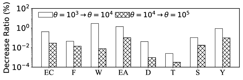
(a) Expected Spread v.s. #Sampled Graphs

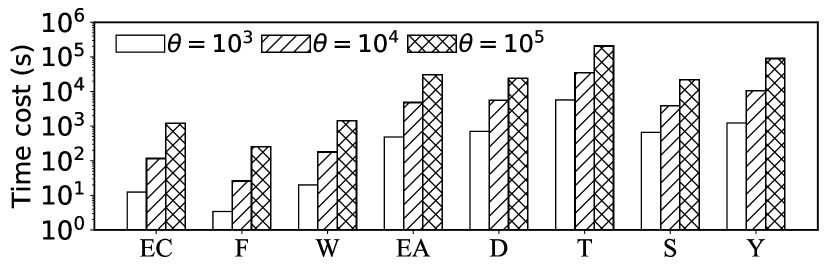
(b) Running Time v.s. Number of Sampled Graphs

Figure A2: Time Cost of Different Algorithms for the IMIN problem under the IC model

References

- Ackermann (1928) Ackermann W (1928) Zum Hilbertschen Aufbau der reellen Zahlen. Math. Ann. 99:118–133.
- Aghaee et al. (2021) Aghaee Z, Ghasemi MM, Beni HA, Bouyer A, Fatemi A (2021) A survey on meta-heuristic algorithms for the influence maximization problem in the social networks. Computing 2437–2477.
- Aho and Ullman (1973) Aho AV, Ullman JD (1973) The theory of parsing, translation, and compiling. 2: Compiling (Prentice-Hall).
- Banerjee et al. (2013) Banerjee A, Chandrasekhar AG, Duflo E, Jackson MO (2013) The diffusion of microfinance. Science 341(6144):1236498.
- Banerjee et al. (2020) Banerjee S, Jenamani M, Pratihar DK (2020) A survey on influence maximization in a social network. Knowl. Inf. Syst. 3417–3455.
- Bhaskara et al. (2010) Bhaskara A, Charikar M, Chlamtac E, Feige U, Vijayaraghavan A (2010) Detecting high log-densities: an O(n) approximation for densest k-subgraph. STOC, 201–210 (ACM).
- Borgs et al. (2014) Borgs C, Brautbar M, Chayes JT, Lucier B (2014) Maximizing social influence in nearly optimal time. SODA, 946–957.
- Budak et al. (2011) Budak C, Agrawal D, Abbadi AE (2011) Limiting the spread of misinformation in social networks. WWW, 665–674.
- Chen et al. (2010) Chen W, Wang C, Wang Y (2010) Scalable influence maximization for prevalent viral marketing in large-scale social networks. KDD, 1029–1038.
- Doerr et al. (2012) Doerr B, Fouz M, Friedrich T (2012) Why rumors spread so quickly in social networks. Commun. ACM 55(6):70–75.
- Domingos and Richardson (2001) Domingos PM, Richardson M (2001) Mining the network value of customers. KDD, 57–66.
- Durrett (1995) Durrett R (1995) Ten lectures on particle systems, 97–201 (Springer Berlin Heidelberg).
- Eckles et al. (2022) Eckles D, Esfandiari H, Mossel E, Rahimian MA (2022) Seeding with costly network information. Operations Research 70(4):2318–2348.
- Gentzkow (2017) Gentzkow HAM (2017) Social media and fake news in the 2016 election. The Journal of Economic Perspectives.
- Granovetter (1978) Granovetter M (1978) Threshold models of collective behavior. American journal of sociology 83(6):1420–1443.
- Günneç et al. (2020) Günneç D, Raghavan S, Zhang R (2020) Least-cost influence maximization on social networks. INFORMS Journal on Computing 32(2):289–302.
- Guo et al. (2020) Guo Q, Wang S, Wei Z, Chen M (2020) Influence maximization revisited: Efficient reverse reachable set generation with bound tightened. SIGMOD, 2167–2181.
- Han et al. (2019) Han K, He Y, Huang K, Xiao X, Tang S, Xu J, Huang L (2019) Best bang for the buck: Cost-effective seed selection for online social networks. IEEE Transactions on Knowledge and Data Engineering 32(12):2297–2309.
- Hoffmann et al. (2020) Hoffmann J, Basu S, Goel S, Caramanis C (2020) Disentangling mixtures of epidemics on graphs. International Conference on Machine Learning (ICML) .
- Ishihata and Sato (2011) Ishihata M, Sato T (2011) Bayesian inference for statistical abduction using markov chain monte carlo. ACML, volume 20, 81–96.
- Johnson et al. (2020) Johnson NF, Velásquez N, Restrepo NJ, Leahy R, Gabriel N, El Oud S, Zheng M, Manrique P, Wuchty S, Lupu Y (2020) The online competition between pro- and anti-vaccination views. Nature 582:230–233.
- Jung et al. (2012) Jung K, Heo W, Chen W (2012) IRIE: scalable and robust influence maximization in social networks. ICDM, 918–923.
- Kempe et al. (2003) Kempe D, Kleinberg JM, Tardos É (2003) Maximizing the spread of influence through a social network. KDD, 137–146.
- Kempe et al. (2005) Kempe D, Kleinberg JM, Tardos É (2005) Influential nodes in a diffusion model for social networks. ICALP, 1127–1138.
- Khot (2006) Khot S (2006) Ruling out PTAS for graph min-bisection, dense k-subgraph, and bipartite clique. SIAM J. Comput. 36:1025–1071.
- Kimura et al. (2008) Kimura M, Saito K, Motoda H (2008) Minimizing the spread of contamination by blocking links in a network. AAAI.
- Kuhlman et al. (2013) Kuhlman CJ, Tuli G, Swarup S, Marathe MV, Ravi SS (2013) Blocking simple and complex contagion by edge removal. ICDM, 399–408.
- Lee et al. (2019) Lee C, Sung C, Ma H, Huang J (2019) IDR: positive influence maximization and negative influence minimization under competitive linear threshold model. MDM, 501–506.