Detection of evolutionary shifts in variance under an Ornstein–Uhlenbeck model

1. Abrupt environmental changes can lead to evolutionary shifts in not only mean (optimal value), but also variance of descendants in trait evolution. There are some methods to detect shifts in optimal value but few studies consider shifts in variance.

2. We use a multi-optima and multi-variance OU process model (Beaulieu, Jhwueng, Boettiger, and O’Meara, 2012) to describe the trait evolution process with shifts in both optimal value and variance and provide analysis of how the covariance between species changes when shifts in variance occur along the path.

3. We propose a new method to detect the shifts in both variance and optimal values based on minimizing the loss function with $\ell_{1}$ penalty. We implement our method in a new R package, ShiVa (Detection of evolutionary shifts in variance).

4. We conduct simulations to compare our method with the two methods considering only shifts in optimal values ($\ell$1ou; PhylogeneticEM). Our method shows strength in predictive ability and includes far fewer false positive shifts in optimal value compared to other methods when shifts in variance actually exist. When there are only shifts in optimal value, our method performs similarly to other methods. We applied our method to the cordylid data ( Broeckhoven, Diedericks, Hui, Makhubo, and Mouton, 2016). ShiVa outperformed $\ell$1ou and phyloEM, exhibiting the highest log-likelihood and lowest BIC.

Keywords— evolutionary shift detection, Ornstein-Uhlenbeck model, LASSO, trait evolution, ensemble method, phylogenetic comparative methods

1 Introduction

The trait evolution process is related to the environment. Abrupt environmental changes for a species might lead to changes in the evolutionary process of the descendants to adapt to the environment (Losos, 2011; Mahler, Ingram, Revell, and Losos, 2013). The changes in the evolutionary process will be reflected in the observed trait values of present-day species. By detecting abrupt changes based on observed traits, we can get knowledge of unobserved historical environmental changes and better understand the evolutionary history. The most popular statistical models to model the evolutionary process along a phylogenetic tree are Brownian Motion (BM, Felsenstein, 1985) and the Ornstein-Uhlenbeck process (Hansen, 1997). Abrupt changes in the evolutionary process are mainly modeled by shifts in parameters in these models. Most research in this area focuses on the detection of shifts in mean (BM model) or optimal value (OU model). Butler and King (2004) formulate the multiple-optima OU model for adaptive evolution. They assume that the optimum is constant along a branch and may differ between branches due to discrete events where changes in selective regime occur. They test the difference in optima between branches using hypothesis testing. Uyeda and Harmon (2014) propose a Bayesian framework to detect shifts in the selective optimum of OU models. Ho and Ané (2014) illustrate the limitation of AIC and BIC in the shift detection task and introduce modified BIC (Zhang and Siegmund, 2006) into the shift detection task. They perform forward-backward selection to conduct model selection. Khabbazian et al. (2016) formulate the shift detection problem into a variable selection problem and combine the OU model with LASSO to detect the shift points, which they implement in the $\ell$1ou R package. The application of LASSO makes it a fast method. Further, they propose a new information criterion pBIC with correction for phylogenetic correlations. Bastide et al. (2017) develop a maximum likelihood estimation procedure based on the EM algorithm, which they implement in the R package PhylogeneticEM. Zhang et al. (2022) propose an ensemble variable selection method (R package ELPASO). They conduct simulations for scenarios when the common model assumptions are violated and show that measurement error, tree construction error and shifts in the diffusion variance impact the performances of the current methods.

However, these methods only consider shifts in optimal values (mean) without considering shifts in variances. In reality, when abrupt environmental shifts occur, they are likely to not only affect the optimal values but also affect the variances of traits. There are some existing models which allow variance ($\sigma^{2}$) to change. Beaulieu et al. (2012) generalize the Hansen model to allow multiple variance parameters and multiple attraction parameters for different selective regimes. Mitov et al. (2020) explore a sub-family of Gaussian phylogenetic models, denoted $\mathcal{G}_{LInv}$, which support models with shifts in variance and propose a fast likelihood calculation algorithm for the family. Bastide et al. (2021) propose a Bayesian inference framework under a Gaussian evolution model that exploits Hamiltonian Monte Carlo (HMC) sampling. The framework allows a variety of models including models with multiple variance parameters. The above models allow changes in variance parameter, but do not incorporate advanced variable selection methods for determining where these shifts in variance occur. In this paper, we propose a method that can simultaneously detect both shifts in optimal value and shifts in variance.

We use a multi-optima and multi-variance OU process model (Beaulieu, Jhwueng, Boettiger, and O’Meara, 2012) to describe the trait evolution process with shifts in both optimal value and variance. We provide analysis of how the covariance between species changes when shifts in variance occur along the path. We then propose a new method to detect both shifts in optimal value and shifts in variance using LASSO. We implement our method in a new R pacakge, ShiVa (Detection of evolutionary shifts in variance). We conduct simulations and compare with $\ell$1ou and PhylogeneticEM. The remainder of the paper is organized as follows. Section 2 introduces the trait evolution model considering shifts in both optimal value and variance, and formulates the shift detection problem. Section 3 describes our algorithm for shift detection. Section 4 presents our simulation results. The methods are compared using both true positive versus false positive curves of shifts in optimal values and predictive log-likelihood. Section 5 illustrates the use of ShiVa with cordylid data (Broeckhoven, Diedericks, Hui, Makhubo, and Mouton, 2016). Section 6 provides the conclusion and discussion.

2 Trait evolution with shifts in both optimal value and variance

2.1 Trait evolution models

The phylogenetic tree is reconstructed from DNA sequences and assumed known in this paper. The phylogenetic tree reveals the correlation structure between trait values of different species. The trait values are correlated based on the shared evolutionary history of species. The trait values of internal nodes are hidden and only trait values of tip nodes can be observed.

Trait evolution models are used to model how the trait values change over time. Brownian Motion and Ornstein–Uhlenbeck are two commonly used models to model the evolution of continuous traits. The BM model is a special case of the OU model. For both models, we let $Y$ denote the vector of observed trait values at the tips, and $Y_{i}$ denote the trait value of taxon $i$. For a single branch, we let $Y_{i}(t)$ denote the trait value at time $t$. These two models assume that conditioning on the trait value of a parent, the evolutionary processes of sister species are independent. We therefore only need to specify the model on one branch. For specifying the model on a single branch, we let $Y(t)$ denote the trait value at time $t$ on a fixed branch.

Brownian Motion Model

Brownian motion (BM) was first introduced to model the evolution of continuous traits over time by Felsenstein (1985). Under this model, The trait value evolves following a BM process. The evolution processes of two species are independent given the trait value of their most recent common ancestor. Therefore, the correlation between the trait values of two species depends only on the evolution time they shared. Based on the properties of the BM process, the observed trait values $\mathrm{Y}$ follow a multivariate Gaussian distribution. For an ultrametric tree of height $1$, each $y_{i}$ has mean $\mu_{0}$ and variance at time $t$, $\sigma^{2}(t)$, so the covariance between $y_{i}$ and $y_{j}$ is $\int_{0}^{t_{ij}}\sigma^{2}(t)dt$, where $t_{ij}$ is the shared evolution time between species $i$ and $j$.

Ornstein–Uhlenbeck Model

(Hansen, 1997) uses an OU process to model the evolutionary process. A selection force that pulls the trait value toward a selective optimum $\theta$ is included in OU models. An OU process $Y(t)$ is defined by the following stochastic differential equation

$$dY(t)=\alpha[\theta(t)-Y(t)]dt+\sigma(t)dB(t)$$

where $dY(t)$ is the infinitesimal change in trait value; $B(t)$ is a standard BM; $\sigma^{2}(t)$ measures the intensity of random fluctuation at time $t$; $\theta(t)$ is the optimal value of the trait at time $t$; and $\alpha\geq 0$ is the selection strength. When $\alpha=0$, the OU process is the same as a BM. We assume that $\alpha$ is constant. For the BM model, the variance of the trait $\int_{0}^{T}\sigma^{2}(t)dt$ is unbounded when $T$ increases. On the other hand, for the OU model, the variance of the trait $\int_{0}^{T}\sigma^{2}(t)e^{-2\alpha(T-t)}dt$ is bounded, which is considered more realistic for most traits. Therefore, compared to the BM model, the OU model is more popular for modeling the evolutionary process.

2.2 Evolutionary shifts in optimal value and variance

Butler and King (2004) formulate the multi-optima OU model for adaptive evolution. This model assumes that the optimal value $\theta(t)$ is constant along a branch and may be different between branches. An abrupt change in $\theta(t)$ on a branch is considered an evolutionary shift in optimal value. However, in most previous work, it is assumed that the variance $\sigma^{2}(t)$ is constant throughout the tree. In reality, when a change in the environment happens, not only the optimal values, but also the variances are likely to change. In this paper, we use a multi-optima multi-variance model (Beaulieu, Jhwueng, Boettiger, and O’Meara, 2012) which allows the variances $\sigma(t)$ to change over different branches.

Solving the OU process equation, the trait value at time $t$ is given by

$$Y_{t}=y_{0}e^{-\alpha t}+\alpha\int_{0}^{t}e^{-\alpha(t-s)}\theta(s)ds+\int_{0}^{t}\sigma(s)e^{-\alpha(t-s)}dW_{s}$$

Solving this, the trait value of species $i$ follows a normal distribution with expectation given by:

$$E(Y_{i})=y_{0}e^{-\alpha T}+\alpha\int_{0}^{T}e^{-\alpha(T-s)}\theta(s)ds$$

By Itô isometry, the element $\Sigma_{i,j}$ (covariance of $Y_{i}$ and $Y_{j}$) of covariance matrix $\Sigma$ is given by

$$\Sigma_{i,j}=e^{-2\alpha(T-t_{a})}\int_{0}^{t_{a}}\sigma^{2}(s)e^{-2\alpha(t_{a}-s)}ds$$

Where $a$ is the separating point of species $i$ and $j$. For ultrametric trees, the distance between i and j is $2t_{ai}=2t_{aj}=2(T-t_{a})$. For shifts in optimal value, Ho and Ané (2014) showed that the exact location and number of shifts on the same branch are unidentifiable. We therefore also assume that the optimal value is constant along a branch. We let $\theta_{b}$ denote the optimal value on branch $b$, $\Delta\theta_{b}$ denote the change in optimal value on branch $b$ and $\operatorname{path}(\textrm{root},i)$ denote the branches on the path of the phylogenetic tree from the root to the tip $i$. The expectation can be writen as the following equation (Khabbazian, Kriebel, Rohe, and Ané, 2016).

$$E(Y_{i})=y_{0}e^{-\alpha T}+(1-e^{-\alpha T})\theta_{0}+\sum_{b\in\operatorname{path}(\textrm{root},i)}(1-e^{-\alpha t_{b}})\Delta\theta_{b}$$

Let $\beta_{0}=y_{0}e^{-\alpha T}+(1-e^{-\alpha T})\theta_{0}$ and $\beta_{b}=(1-e^{-\alpha t_{b}})\Delta\theta_{b}$. Then,

$$E(Y_{i})=\beta_{0}+\sum_{b}\beta_{b}\mathbf{X_{bi}}$$ (1)

where $X_{b}$ is a vector defined by $X_{bi}=0$ if taxon $i$ is not under branch $b$, and $X_{bi}=1$ if the taxon $i$ is under branch $b$.

While shifts in optimal value only affect the expectation of the $Y_{i}$, shifts in variance affect the variance of $Y_{i}$ and the covariance of $Y_{i}$ and $Y_{j}$. In particular, if species $i$ and $j$ separate at time $t_{a}$, and the shifts in variance along the shared evolutionary path occur at times $t_{1},\ldots,t_{m}$, with magnitudes $\Delta\sigma_{1}^{2},\Delta\sigma_{2}^{2},\ldots,\Delta\sigma_{m}^{2}$ respectively, then the covariance $\Sigma_{ij}$ is given by

$$\Sigma_{i,j} =\frac{e^{-2\alpha(T-t_{a})}}{2\alpha}\left((1-e^{-2\alpha t_{a}})\sigma^{2}_{0}+\sum_{l\in\operatorname{path}(\textrm{root},a)}\left(1-e^{-2\alpha\left(t_{a}-t_{l}\right)}\right)\Delta\sigma^{2}_{l}\right)$$

The results of Ho and Ané (2014) about the unidentifiability of shift positions along a branch are not completely applicable for shifts in variance. By examining the covariance between pairs of species under a given branch, we can estimate the covariance at the end of the branch, and from their mean, we can estimate the trait value at the end of the branch. This can result in different likelihoods for different positions of a single shift on a branch, so the position is identifiable. For example, considering the species $i,j,k,l$ on the following tree:

for tree= grow = east, parent anchor=east, child anchor=west, align=center, tier/.wrap pgfmath arg=tier #1level(),if n children=0tier=word,font=, [a [a’ [a” [l ][k ]][j ]][i ]]

With a single shift in variance on the branch from a to a’, we have the following equations to solve for the time and magnitude of the shift.

$$\Sigma_{jk}-\Sigma_{ij}=\sigma_{0}^{2}/2\alpha(e^{-2\alpha(T-t_{a^{\prime}})}-e^{-2\alpha(T-t_{a})})+\Delta\sigma^{2}/2\alpha(e^{-2\alpha(T-t_{a^{\prime}})}-e^{-2\alpha(T-t_{a})})$$

$$\Sigma_{kl}-\Sigma_{jk}=\sigma_{0}^{2}/2\alpha(e^{-2\alpha(T-t_{a^{\prime\prime}})}-e^{-2\alpha(T-t_{a^{\prime}})})+\Delta\sigma^{2}/2\alpha(e^{-2\alpha(T-t_{a^{\prime\prime}})}-e^{-2\alpha(T-t_{a^{\prime}})})$$

which can easily be seen to be solveable for both $\Delta\sigma^{2}$ and $t$. However, the times, magnitudes and even number of shifts will be unidentifiable if there are two (or more) shifts on the same branch. For example, if there are shifts in variance at times $t_{1}$ and $t_{2}$ on branch $b$, with magnitudes $\Delta\sigma_{1}^{2}$ and $\Delta\sigma_{2}^{2}$ respectively, then for any two species below branch $b$, their covariance will include the term $\frac{e^{-2\alpha(T-t_{a})}}{2\alpha}\left(1-e^{-2\alpha\left(t_{a}-t_{1}\right)}\right)\Delta\sigma^{2}_{1}+\frac{e^{-2\alpha(T-t_{a})}}{2\alpha}\left(1-e^{-2\alpha\left(t_{a}-t_{2}\right)}\right)\Delta\sigma^{2}_{2}$. Thus it is not possible to seperate $\Delta\sigma_{1}^{2}$ and $\Delta\sigma_{2}^{2}$, or $t_{1}$ and $t_{2}$. Indeed, in many cases, there is a single shift on branch $b$ that would produce the same covariance matrix.

For model and computational simplicity, we assume that $\sigma^{2}$ is constant over a branch like the assumption for $\theta$. That is, we assume that any shift in variance on a branch occurs at the beginning of that branch. For shifts in mean, this assumption did not limit the space of possible models due to the unidentifiability. However, for shifts in variance, this does restrict the space of models for the trait values at the leaves, and could therefore adversely affect shift detection. We will study whether this adverse effect is cause for concern in our simulation studies. Under our assumptions, we let $\sigma^{2}_{b}$ denote the variance on the branch $b$, $\Delta\sigma^{2}_{b}$ denote the magnitude of shift in variance on the branch $b$: if no shift occurs on the branch $b$, $\Delta\sigma^{2}_{b}=0$. The covariance between species $i$ and $j$ is given by:

$$\Sigma_{i,j} =\frac{e^{-2\alpha(T-t_{a})}}{2\alpha}\left((1-e^{-2\alpha t_{a}})\sigma^{2}_{0}+\sum_{b\in\operatorname{path}(\textrm{root},a)}(1-e^{-2\alpha\left(t_{a}-t_{b}\right)})\Delta\sigma^{2}_{b}\right)$$

$$=\frac{e^{-2\alpha(T-t_{a})}}{2\alpha}\left((1-e^{-2\alpha t_{a}})\sigma^{2}_{0}+\sum_{b\in\operatorname{path}(\textrm{root},a)}\left(1-e^{-2\alpha t_{a}}+e^{-2\alpha t_{a}}-e^{-2\alpha\left(t_{a}-t_{b}\right)}\right)\Delta\sigma^{2}_{b}\right)$$

$$=\frac{e^{-2\alpha(T-t_{a})}}{2\alpha}\left((1-e^{-2\alpha t_{a}})\sigma^{2}_{0}+\sum_{b\in\operatorname{path}(\textrm{root},a)}\left((1-e^{-2\alpha t_{a}})+e^{-2\alpha t_{a}}(1-e^{2\alpha t_{b}})\right)\Delta\sigma^{2}_{b}\right)$$

$$=\frac{e^{-2\alpha(T-t_{a})}}{2\alpha}\left(1-e^{-2\alpha t_{a}}\right)\sigma^{2}_{0}+\sum_{b\in\operatorname{path}(\textrm{root},a)}\frac{e^{-2\alpha(T-t_{a})}}{2\alpha}(1-e^{-2\alpha t_{a}})\Delta\sigma^{2}_{b}$$

$$\qquad+\sum_{b\in\operatorname{path}(\textrm{root},a)}\frac{e^{-2\alpha T}}{2\alpha}\left(1-e^{2\alpha t_{b}}\right)\Delta\sigma^{2}_{b}$$ (2)

For the ancestral state at the root node, two different assumptions are commonly used, fixed value or stationary distribution. We assume that the ancestral state at the root is a fixed value for the above process. Equation 2.2 is the covariance of node $i$ and $j$ for the OU model with fixed root. For the OU model, the ancestral state at the root is also often assumed to have the stationary distribution. In this case, the covariance of the root node is $\sigma_{0}^{2}/(2\alpha)$ (Ho and Ané, 2013). In this case, the covariance with shifts can be written as:

$$\Sigma_{i,j} =\frac{e^{-2\alpha(T-t_{a})}}{2\alpha}\left(1-e^{-2\alpha t_{a}}\right)\sigma^{2}_{0}+\sum_{b\in\operatorname{path}(\textrm{root},a)}\frac{e^{-2\alpha(T-t_{a})}}{2\alpha}(1-e^{-2\alpha t_{a}})\Delta\sigma^{2}_{b}$$

$$\qquad+\sum_{b\in\operatorname{path}(\textrm{root},a)}\frac{e^{-2\alpha T}}{2\alpha}\left(1-e^{2\alpha t_{b}}\right)\Delta\sigma^{2}_{b}+\frac{e^{-2\alpha T}}{2\alpha}\sigma_{0}^{2}$$

$$=\frac{e^{-2\alpha(T-t_{a})}}{2\alpha}\sigma^{2}_{0}+\sum_{b\in\operatorname{path}(\textrm{root},a)}\frac{e^{-2\alpha(T-t_{a})}}{2\alpha}(1-e^{-2\alpha t_{a}})\Delta\sigma^{2}_{b}$$

$$\qquad+\sum_{b\in\operatorname{path}(\textrm{root},a)}\frac{e^{-2\alpha T}}{2\alpha}\left(1-e^{2\alpha t_{b}}\right)\Delta\sigma^{2}_{b}$$

Let $\gamma_{b}=\Delta\sigma_{b}^{2}$, $\mathbf{V}_{i,j}=\frac{e^{-2\alpha(T-t_{a})}}{2\alpha}(1-e^{-2\alpha t_{a}})$, $\mathbf{U}_{i,j}=\frac{e^{-2\alpha(T-t_{a})}}{2\alpha}$, $q_{b}=\frac{e^{-2\alpha T}}{2\alpha}\left(1-e^{2\alpha t_{b}}\right)$; $\gamma_{b}$ is the shift in variance on branch $b$, $\mathbf{V}$ is the phylogenetic covariance matrix when $\sigma^{2}=1$ (no shift in variance) with fixed root, $\mathbf{U}$ is the phylogenetic covariance matrix when $\sigma^{2}=1$ (no shift in variance) with stationary distributed root. $\mathbf{U}$ and $\mathbf{V}$ only depend on the phylogeny. The covariance between species $i$ and $j$ can be expressed as the following equation.

$$\Sigma_{i,j}=\begin{cases}\mathbf{V}_{i,j}\sigma_{0}^{2}+\sum_{b}\gamma_{b}X_{ib}X_{jb}\mathbf{V}_{i,j}+\sum_{b}\gamma_{b}q_{b}X_{ib}X_{jb}&\text{OU model with fixed root}\\ \mathbf{U}_{i,j}\sigma_{0}^{2}+\sum_{b}\gamma_{b}X_{ib}X_{jb}\mathbf{V}_{i,j}+\sum_{b}\gamma_{b}q_{b}X_{ib}X_{jb}&\text{OU model with random root}\end{cases}$$

It consists of 3 terms. The first term is the original covariance without any shift. The last 2 terms show the influence of shifts in variances. In addition to the shift sizes $\gamma_{b}$, the second term is influenced by the phylogentic structure ($\mathbf{V}_{i,j}$), higher original covariance between two species leads to larger change in covariance for a fixed shift size (Figure 2); the third term is influenced by the start time of branch b ($\mathbf{q}_{b}$), earlier shifts lead to larger change in covariance between two species (Figure 2).

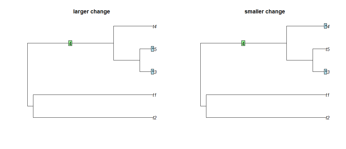
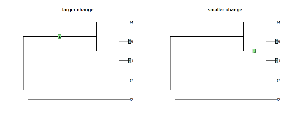
Figure 1: Higher original covariance between two species leads to larger change in covariance for the same shift magnitude: larger change for the shift in the left figure

Figure 2: Earlier shift leads to larger change in covariance for a given species: larger change for the shift in the left figure

For simplicity, we let $\mathbf{R}$ denote the phylogenetic covariance matrix when there is no shift in variance and $\sigma^{2}_{0}=1$. So $\mathbf{R=V}$ when the root is fixed and $\mathbf{R=U}$ when the trait value at the root follows the stationary distribution.

Using matrix notation, the covariance matrix can be expressed as:

$$\mathbf{\Sigma} =\sigma_{0}^{2}\mathbf{R}+\left(\sum_{b=1}^{p}\gamma_{b}\mathbf{X_{b}X_{b}^{T}}\right)\odot\mathbf{V}+\sum_{b=1}^{p}\gamma_{b}q_{b}\mathbf{X_{b}X_{b}^{T}}$$

$$=\sigma_{0}^{2}\mathbf{R}+\left(\mathbf{X}\operatorname{diag}(\gamma)\mathbf{X^{T}}\right)\odot\mathbf{V}+\mathbf{X}\operatorname{diag}(\gamma\odot q)\mathbf{X^{T}}$$ (3)

Where $\odot$ represents elementwise multiplication of matrices and vectors. The trait values at tips can be written as:

$$\mathbf{Y}=\beta_{0}\mathbf{1}+\sum_{b}\beta_{b}\mathbf{X_{b}}+\mathbf{\epsilon}$$

Where $\epsilon$ follows a normal distribution with mean 0 and covariance matrix $\Sigma$, given by Equation 2.2. The main task is to select the branches that have $\beta_{b}\neq 0$ and $\gamma_{b}\neq 0$; and estimate the values of $\beta_{b}$ and $\gamma_{b}$.

3 Methods

In this section, we propose a new method to simultaneously detect the shifts in both variance and optimal values based on minimizing the loss function with L1 penalty. When $Y$ follows a multivariate normal distribution with mean and variance given by Equations 1 and 2.2, the log likelihood is

$$L(\beta,\gamma) =-\frac{1}{2}(\mathbf{Y}-\beta_{0}-\mathbf{X}\mathbf{\beta})^{T}\mathbf{\Sigma}^{-1}(\mathbf{Y}-\beta_{0}-\mathbf{X}\mathbf{\beta})-\frac{1}{2}\log{\det{(\mathbf{\Sigma})}}$$

$$=-\frac{1}{2}(\mathbf{Y}-\beta_{0}-\mathbf{X}\mathbf{\beta})^{T}\left(\sigma_{0}^{2}\mathbf{R}+\left(\mathbf{X}\operatorname{diag}(\gamma)\mathbf{X^{T}}\right)\odot\mathbf{V}+\mathbf{X}\operatorname{diag}(\gamma\odot q)\mathbf{X^{T}}\right)^{-1}(\mathbf{Y}-\beta_{0}-\mathbf{X}\mathbf{\beta})$$

$$\qquad-\frac{1}{2}\log{\det{\left(\sigma_{0}^{2}\mathbf{R}+\left(\mathbf{X}\operatorname{diag}(\gamma)\mathbf{X^{T}}\right)\odot\mathbf{V}+\mathbf{X}\operatorname{diag}(\gamma\odot q)\mathbf{X^{T}}\right)}}$$

To select the shifts in optimal values ($\beta_{i}\neq 0$) and the shifts in variances ($\gamma_{i}\neq 0$), we use an L1 penalty in the loss function to conduct the feature selection as in LASSO. Therefore, the loss function to be optimized is given by:

$$L(\beta_{1},...,\beta_{p},\gamma_{1},...,\gamma_{p}) =l(\beta_{1},...,\beta_{p},\gamma_{1},...,\gamma_{p};\textbf{Y})+\text{Penalty}$$

$$=\frac{1}{2}(\mathbf{Y}-\beta_{0}-\mathbf{X}\mathbf{\beta})^{T}\left(\sigma_{0}^{2}\mathbf{R}+\left(\sum_{i=1}^{p}\gamma_{i}\mathbf{X_{i}X_{i}^{T}}\right)\odot\mathbf{V}+\sum_{i=1}^{p}\gamma_{i}q_{i}\mathbf{X_{i}X_{i}^{T}}\right)^{-1}$$

$$\qquad(\mathbf{Y}-\beta_{0}-\mathbf{X}\mathbf{\beta})+\frac{1}{2}\log{\det{\left(\sigma_{0}^{2}\mathbf{R}+\left(\sum_{i=1}^{p}\gamma_{i}\mathbf{X_{i}X_{i}^{T}}\right)\odot\mathbf{V}+\sum_{i=1}^{p}\gamma_{i}q_{i}\mathbf{X_{i}X_{i}^{T}}\right)}}$$

$$\qquad+\lambda_{1}\|\beta\|_{1}+\lambda_{2}\|\gamma\|_{1}$$ (4)

3.1 Optimization

We assume that $\alpha$ is known in this paper. The objective here is to find $\mathbf{\beta}$, $\mathbf{\gamma}$ and $\sigma_{0}^{2}$ that minimize Equation 3. When $\mathbf{\gamma}$ is fixed, it can be transformed into a basic LASSO problem. For the optimization of $\mathbf{\gamma}$, we adopt coordinate proximal gradient descent (Parikh, 2014). The proximal gradient algorithm is commonly used to solve non-differentiable convex optimization problems. The objective function is usually broken into two parts: a differentiable part and a non-differentiable part to apply the proximal gradient algorithm. For the optimization, a proximal operator is used to reduce the non-differentiable part.

The loss function for $\gamma_{k}$ can be written as:

$$L(\gamma_{k})=g(\gamma_{k})+\lambda_{2}\|\gamma_{k}\|$$

The derivative of $g(\gamma_{k})$ is given by:

$$\left(\nabla g(\gamma)\right)_{k} =-\frac{1}{2}\mathbf{r}^{T}\mathbf{\Sigma^{-1}}\left(\mathbf{\left(X_{k}X_{k}^{T}\right)}\odot\mathbf{V}\right)\mathbf{\Sigma^{-1}}\mathbf{r}-\frac{1}{2}q_{k}\|\mathbf{X_{k}^{T}\Sigma^{-1}r}\|^{2}+\frac{1}{2}\operatorname{tr}\left(\left(\mathbf{\left(X_{k}X_{k}^{T}\right)}\odot\mathbf{V}\right)\mathbf{\Sigma}^{-1}\right)$$

$$\qquad+\frac{1}{2}q_{k}\mathbf{X_{k}^{T}\Sigma^{-1}X_{k}}$$

where $\mathbf{r}=\mathbf{Y}-\beta_{0}-\mathbf{X^{T}}\mathbf{\beta}$. The proximal operator is given by:

$$\text{prox}_{\lambda_{2}h}(z)=S_{\lambda_{2}}(z)=\begin{cases}z-\lambda_{2}&z>\lambda_{2}\\ 0&-\lambda\leq z\leq\lambda_{2}\\ z+\lambda_{2}&z<-\lambda\end{cases}$$

The proximal algorithm here steps in the direction $\nabla g(\gamma)$ but setting any values that are close to zero equal to zero. For $\sigma^{2}_{0}$, there is no penalty on the parameter. Therefore, we use gradient descent to update $\sigma_{0}^{2}$. The gradient of $\sigma_{0}^{2}$ is given by:

$$\frac{\partial L}{\partial\sigma_{0}^{2}} =-\frac{1}{2}\mathbf{r^{T}}\mathbf{\Sigma}^{-1}\mathbf{R}\mathbf{\Sigma}^{-1}\mathbf{r}+\frac{1}{2}\text{tr}\left(\mathbf{R}\mathbf{\Sigma}^{-1}\right)$$

We initialize $\beta$ and $\gamma$ as 0. In each iteration, we first update the covariance matrix $\Sigma$ and transform $\mathbf{X}$ and $\mathbf{Y}$ with the current $\Sigma^{-1/2}$. Then we update $\beta$ by applying LASSO on the transformed data. Then we update $\gamma$ using the proximal algorithm in an elementwise manner. After that, we update $\sigma_{0}^{2}$ using gradient descent. The algorithm is summarized in Algorithm 1.

Algorithm 1 Optimization with $\beta$, $\gamma$ and $\sigma_{0}^{2}$

1:Inputs:

2:      $M$: maximum number of steps; $t$: step size; $\epsilon$: error tolerance; $\mathbf{V}$; $\mathbf{R}$; $\mathbf{Y}$; $\mathbf{X}$

3:Initialize:

4:      $\beta_{i}^{0}\leftarrow 0$, $i=1,\ldots,p$ $\gamma_{i}^{0}\leftarrow 0$, $i=1,\ldots,p$ $\sigma_{0}^{2}\leftarrow 1$

5:for s = 1 to M do

6:    $\mathbf{\Sigma}\leftarrow\sigma_{0}^{2}\mathbf{R}+\left(\sum_{i=1}^{p}\gamma_{i}\mathbf{X_{i}X_{i}^{T}}\right)\odot\mathbf{V}+\sum_{i=1}^{p}\gamma_{i}q_{i}\mathbf{X_{i}X_{i}^{T}}$

7:    $\mathbf{Y^{\prime}}=\mathbf{\Sigma^{-1/2}Y}$; $\mathbf{X^{\prime}}=\mathbf{\Sigma^{-1/2}X}$

8:    $\beta\leftarrow LASSO(\mathbf{Y^{\prime}},\mathbf{X^{\prime}})$

9:    for k = 1 to p do

10:       calculate $\left(\nabla g(\gamma)\right)_{k}$

11:       update $\gamma_{k}\leftarrow S_{\lambda_{2}t}(\gamma_{k}-t\nabla g(\gamma_{k}))$

12:       update $\mathbf{\Sigma}$

13:    end for

14:    calculate the gradient for $\sigma_{0}^{2}$: $\frac{\partial L}{\partial\sigma_{0}^{2}}$

15:    update $\sigma_{0}^{2}\leftarrow\sigma_{0}^{2}-t\frac{\partial L}{\partial\sigma_{0}^{2}}$

16:    if max update for $\beta$, $\gamma$ and $\sigma_{0}^{2}$ in the iteration $<\epsilon$ then

17:       break

18:    end if

19:end for

3.2 Model selection

We have two tuning parameters ($\lambda_{1}$ and $\lambda_{2}$). Because of the efficiency of computing the LASSO path in regression models, we can efficiently tune $\lambda_{1}$ by cross-validation. So for each fixed $\lambda_{2}$ value, we set $\lambda_{1}$ to 0 to obtain an estimation of the covariance matrix. Then we tune $\lambda_{1}$ by cross validation according to the estimated coariance matrix. We then use BIC to select the best value of $\lambda_{2}$.

4 Simulations

We conduct simulations to test the effectiveness of our method to detect the true shifts in the variance without losing too much accuracy in detecting the shifts in the optimal value. Results of Bayesian approaches are deeply influenced by prior distributions and the computation cost is relatively high. Therefore, we only compare our results with frequentist approaches in this paper. We compare our method with l1ou+pBIC, l1ou+BIC, and phyloEM in the simulations (Khabbazian, Kriebel, Rohe, and Ané, 2016; Bastide, Mariadassou, and Robin, 2017). For the measurement of performance, we consider the True positive and False positive rates for detecting the shifts in variance and optimal values. However, in shift detection, model identification problems can occur. A surrogate shift is a shift on the branch near the true shift (for example, shift on the branch of the parent node or the child node). It influences similar species as the true shift. Selecting a surrogate shift of the true shift could give better inference and prediction than selecting no shift. However, simply counting true positives and false positives might not give sufficient credit for selecting the surrogate shift. Therefore, we also use predictive log-likelihood difference from the true model to evaluate the method performances. For each simulation, we generate $1000$ test datasets and $100$ training datasets. We calculate the mean of log likelihood values over $1000$ test datasets using the estimated shifts from training sets. When the results of a method give higher predictive log-likelihood value, it indicates that the method performs better at predicting the trait values. In order to compare the results across different scenarios, we also calcualte the predictive log-likelihood of the true model, and finally calculate the difference in predictive log-likelihood between each method and the true model. Smaller predictive log-likelihood difference shows smaller gap between the results and the true model, indicating better prediction performance. We use OU model with fixed root to calculate the likelihood.

We simulate datasets under OU models along the 100-taxon Anolis lizards tree (Mahler, Ingram, Revell, and Losos, 2013). We consider 3 different scenario settings; only shifts in variance, only shifts in optimal value and both shifts in optimal value and shifts in variance. For each parameter setting, 100 simulations are conducted. For all simulations, we set $\alpha=1$ and $\sigma_{0}^{2}=2$. Since our method does not support the estimation of $\alpha$, we assume that the correct $\alpha$ value is known for all the methods.

4.1 Case I: Only shifts in variance

The first scenario setting is that only shifts in variance exist in the OU model — the optimal value is constant throughout the tree. We perform a number of simulation studies with a single shift in variance, and compare the detection results when the shift occurs in different positions.

The left figure of Figure 3 shows the different shift positions we set. The right figure of Figure 3 shows the true positive and false positive rates for each shift position. We see that shifts in positions near the root are easier to detect, which is consistent with our analysis in Section 2. When the shift contains a sufficient number of tips and the signal size is large enough, our method has the ability to detect the true shift.

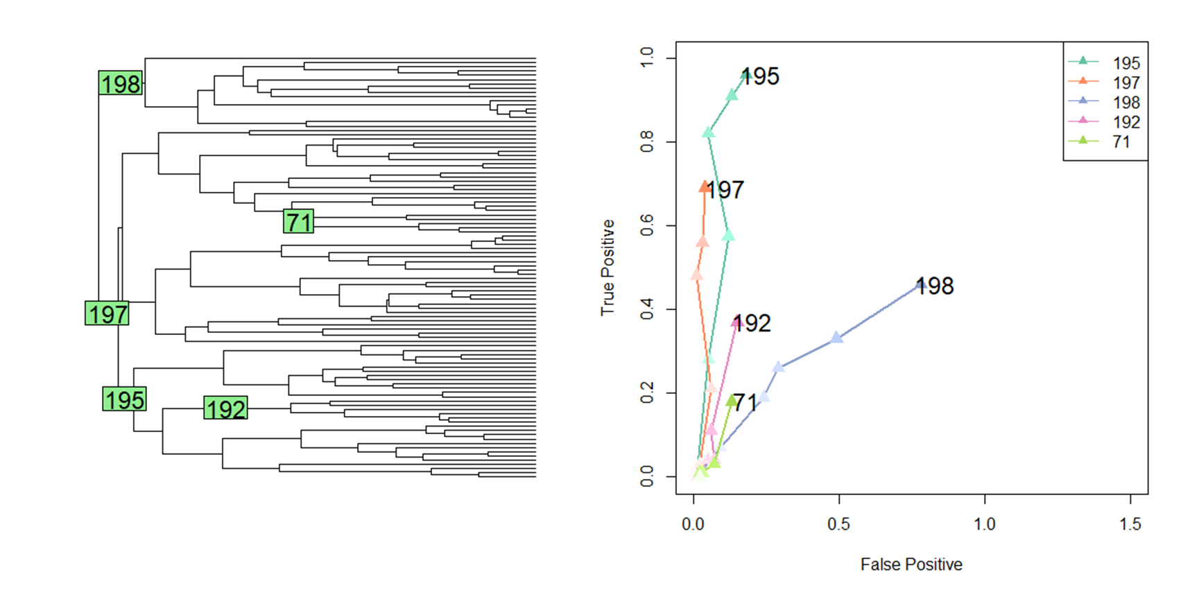
Figure 3: The true positive v.s. false positive rates of our method when there are only shifts in variance

Since there is no true shift in optimal value in this scenario, we here compare the false positive shifts detected in optimal values from different methods. From Figure 4, when the shift in variance has a sufficient number of tips below it (Shift 195) and the shift size is large enough, other methods will detect many false positives in optimal values by misinterpreting the signal as shifts in optimal value. However, our method can successfully detect the true shifts in variance in these cases, so that the false positive numbers for shifts in optimal value can be effectively controlled. The plots of other shift settings show similar patterns and are in the supplemental materials.

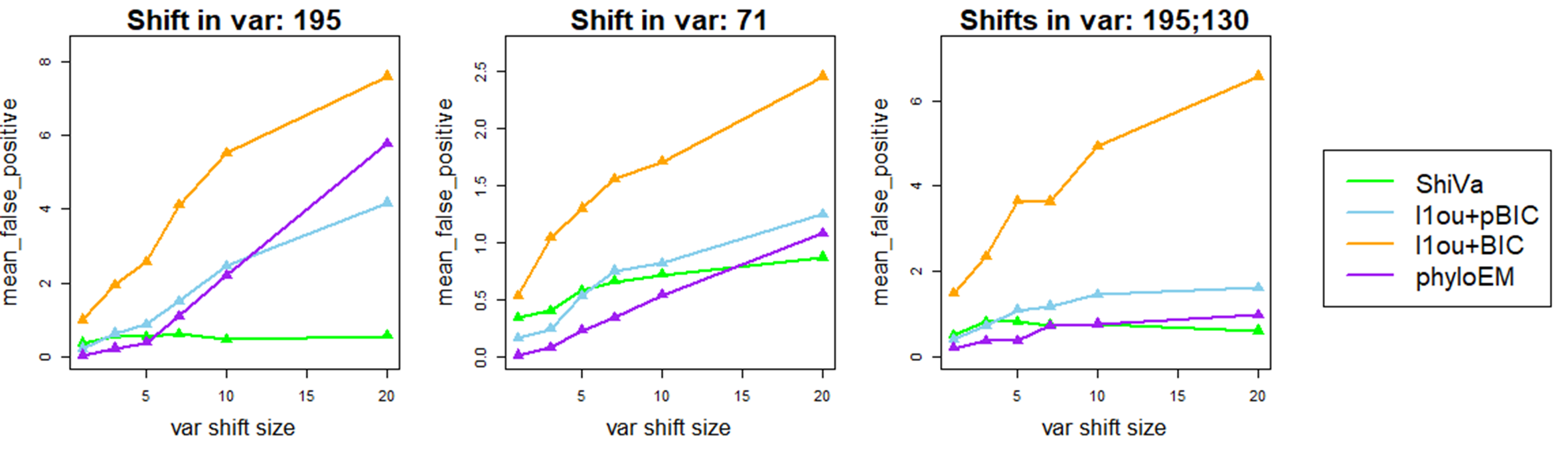
Figure 4: The false positive rates of different methods for detecting shifts in optimal value when there are only shifts in variance

Finally, We compare the predictive log-likelihood difference with the true model for each method. Figure 5 shows that the predictive log likelihood difference is smaller for our method than other methods, especially when the signal size is large and the shifts are near the root. This shows that our method has better predictive ability than other methods when there are only shifts in variance.

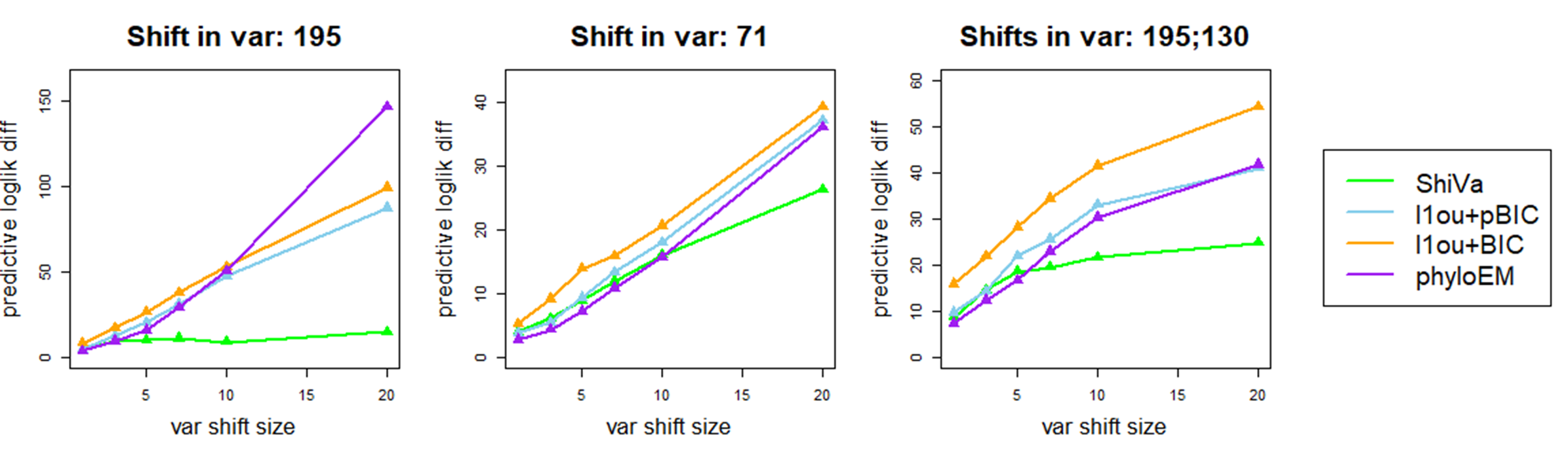
Figure 5: The predictive log-likelihood difference of different methods when there are only shifts in variance

4.2 Case II: Only shifts in optimal value

Simulations are conducted under scenarios with 1, 3, 7, or 12 shifts. The results are shown in Figures 6, 7 and 8. From Figure 6, we see that ShiVa shows no significant weakness in detecting the true shifts in variance. Furthermore, ShiVa generally detects fewer false positives even when there are no shifts in optimal value to mislead the other methods. We also check the number of false positive shifts in variance under our method. Figure 7 shows that the number of false positives is limited. By comparing the predictive log-likelihood difference with true models, we find that our method performs worse than other methods when the number of shifts is large and the shift sizes are large. However, the gap between our method and the other methods is not substantial.

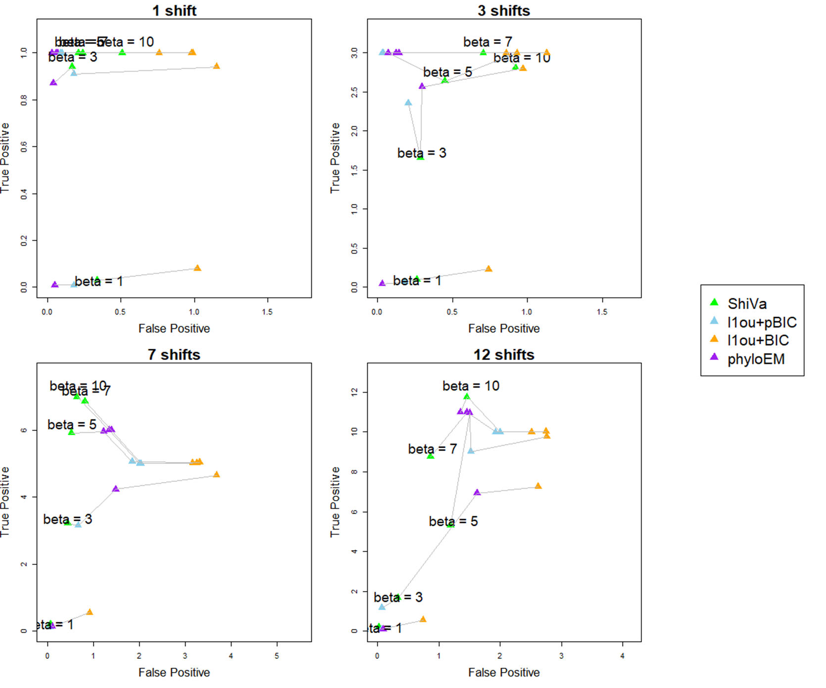
Figure 6: The true positive v.s. false positive rates of different methods when there are only shifts in optimal value

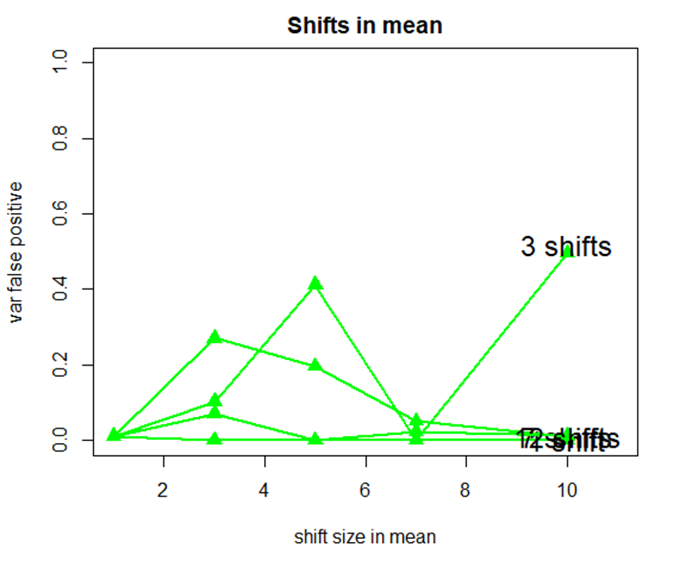
Figure 7: The false positive rates of the new method for shifts in variance when there are only shifts in optimal value

Figure 8: The predictive log-likelihood difference of different methods when there are only shifts in optimal value

4.3 Case III: Both shifts in optimal value and shifts in variance

We simulate one shift in optimal value and one shift in variance. We consider three different relationships between the shift in optimal value and the shift in variance: the shifts are on independant lineages; the shift in variance is ancestral to the shift in optimal value; and the shift in optimal value is ancestral to the shift in variance. The simulated shift configurations are shown in Figure 9.

Figure 10 shows the true positive and false positive rate for each method in each scenario for detecting shifts in optimal value. Overall, our method has much fewer false positives for shifts in optimal value than other methods. All the other methods have very high false positive rates since they wrongly detect the shift in variance as many different shifts in the optimal value. In addition to controlling the false positive rates, ShiVa performs generally well in terms of detecting the true positive shifts in optimal value except for limited cases. Figure 12 compares the predictive log-likelihood for each method in these scenarios. We see that our method has the smallest predictive log-likelihood difference from the true model. This shows that when there are shifts in variance, even if there are also shifts in optimal value, ShiVa selects better predictive models than methods that only select shifts in optimal value.

Figure 11 shows the true positive and false positive rate of ShiVa for shifts in variance. In order to show how the magnitudes of shift in variance and shift in optimal value influence the shift detection results, we keep the magnitude of shift in optimal value as 10 and vary magnitude of shift in variance in the left plot; and we keep the magnitude of shift in variance as 20 and vary magnitude of shift in optimal value in the right plot. It shows that when the shift in optimal value is under the shift in variance, the shift in variance is easiest to detect. When the shift in variance is under the shift in mean, the shift in variance is hardest to detect. Furthermore, when the signal size of shift in variance is much larger than the signal size of shift in optimal value, ShiVa has better performance with higher true positive rates and lower false positive rates.

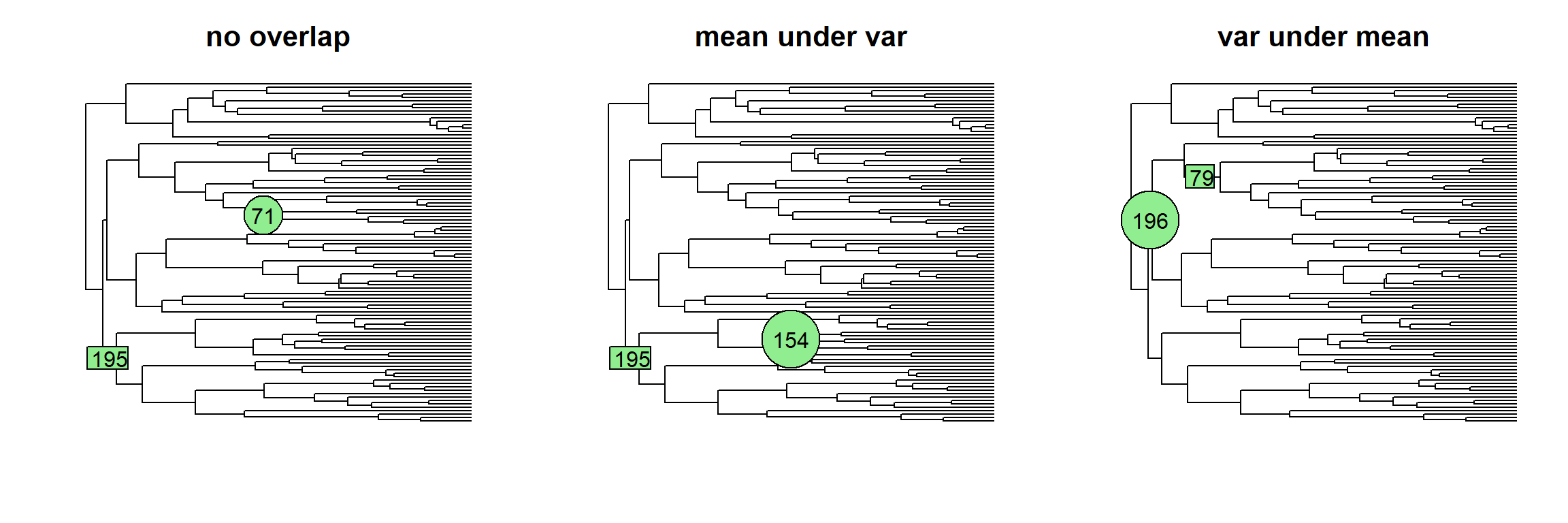
Figure 9: Shift configurations of the simulations. Circle: shift in optimal value; Rectangle: shift in variance

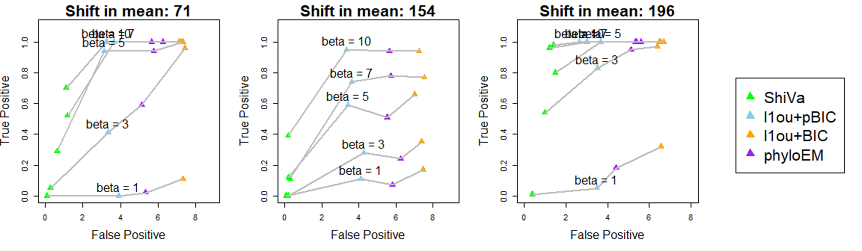
Figure 10: The true positive v.s. false positive rates of different methods for shifts in mean when there are both shifts in variance and optimal value

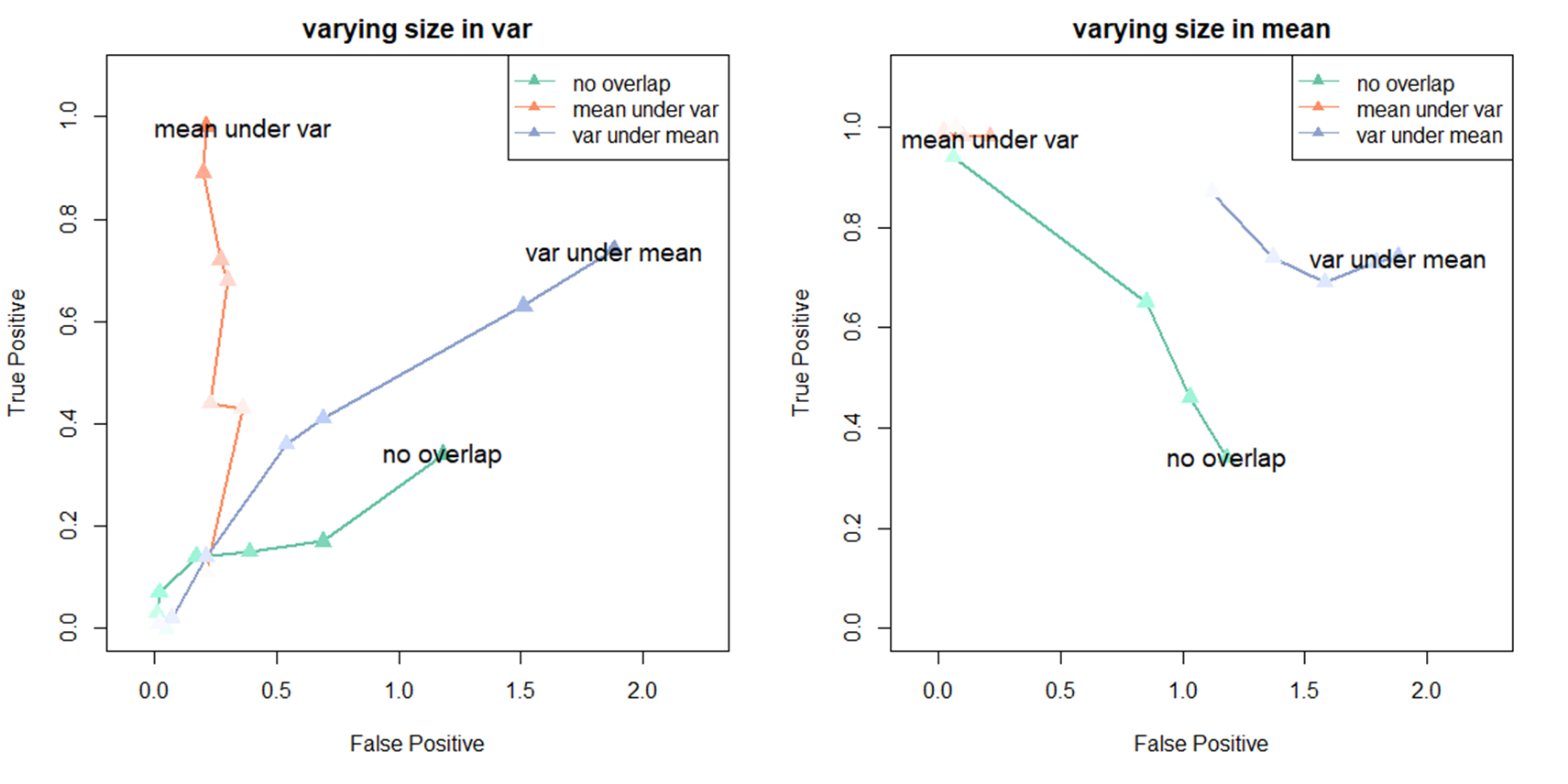
Figure 11: The true positive v.s. false positive rates of ShiVa for shifts in variance when there are both shifts in variance and optimal value. Left: Vary magnitude of shift in variance. Right: Vary magnitude of shift in optimal value

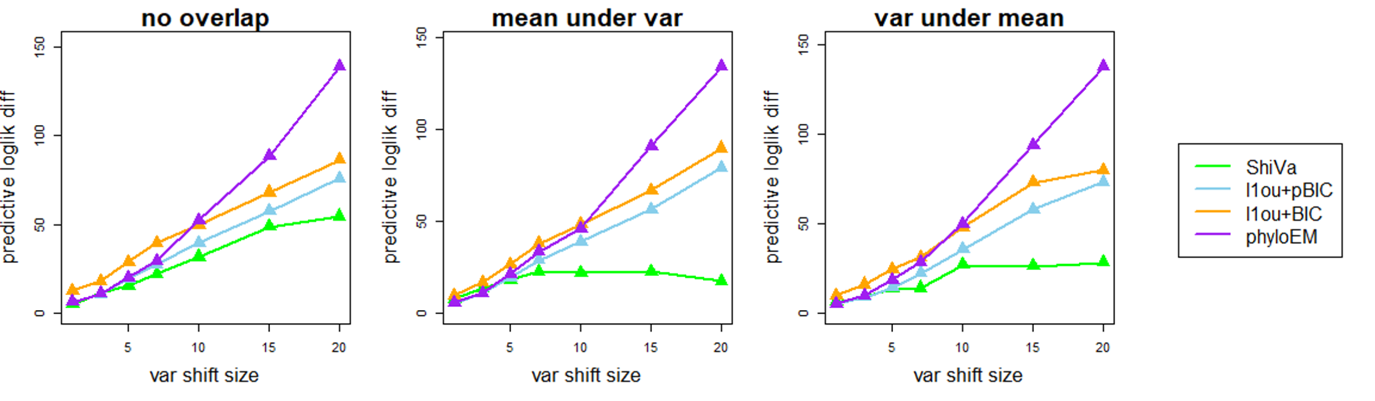
Figure 12: The predictive log-likelihood difference of different methods when there are both shifts in variance and optimal value

4.4 Discussion about assumption violations

In Section 2, we noted that our assumptions about the shifts in variance—at most one shift will occur on any branch; and the shifts occur at the beginning of the branches—are restrictions on the space of possible models, so in particular if these assumptions are not satisfied, then the model is misspecified. In this subsection, we conduct simulations in which these assumptions are violated.

Firstly, we conduct a series of simulations with the shift occuring in different positions along a fixed branch. The different locations of shift are shown in Figure 13 (left). Figure 14 shows the false positive v.s. true positive rates and the predictive log-likelihood difference of the new method with shifts in different locations. Location here is a parameter ranging from 0 to 1, with 0 meaning the beginning of the branch and 1 meaning the end of the branch. The ability of the method to detect the shift in variance is not greatly impacted by the position of the shift along the branch. Furthermore, when the shift size is small, the log-likelihood of the model is not much reduced in situations where the location of the shift is not at the beginning of the branch. However, when the magnitude of the shift is larger, the model misspecification does cause a substantial decrease in log-likelihood when the shift is not located at the begining of the branch. Overall, our method is robust to violations of our assumption that shifts occur at the beginning of a branch.

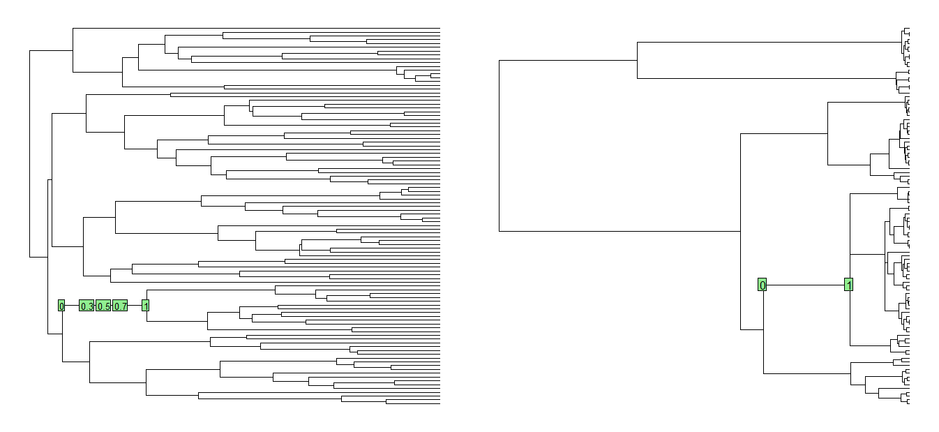
Figure 13: Left: The different locations of shifts on the same branch; Right: Two opposite shifts occur on the same branch

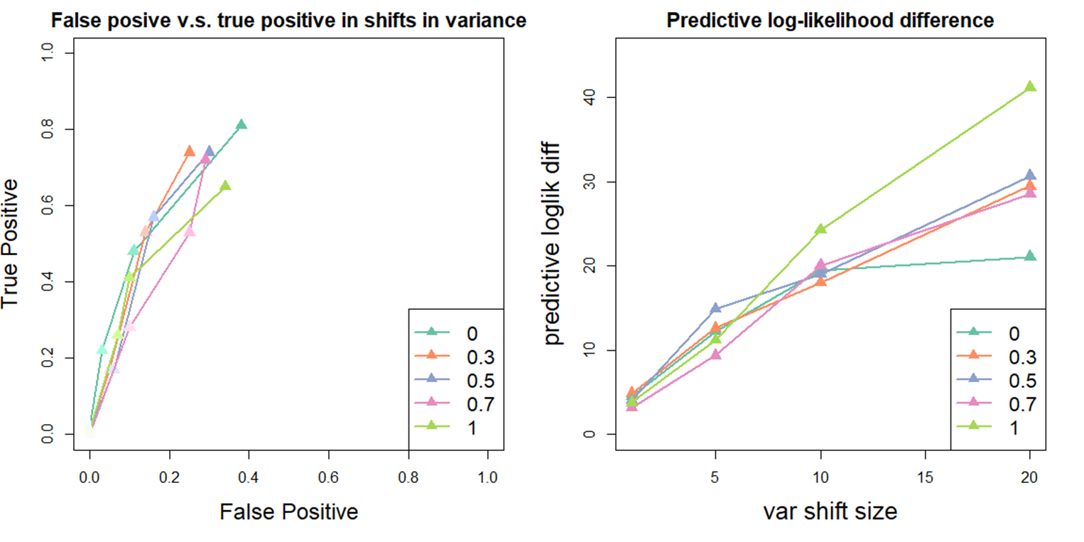
Figure 14: The true positive v.s. false positive rates and the predictive log-likelihood difference of ShiVa with shifts at different locations

Secondly, we simulate scenarios with two shifts on a single branch. If shifts are both positive or both negative, the data will show a stronger signal than when just one shift occurs. Therefore, we simulate situations where two opposite shifts occur (at locations = 0 and 1) (Figure 13 right). To compare, we also simulate situations where only one shift occurs at the beginning of that branch. Table 1 shows that when the two opposite shifts occur on that branch, our method cannot accurately detect the shift in variance on that branch and the false positive rate of shifts in optimal value increases. In this case, the violation of the assumption causes some difficulties for our method. However, in the general case, it is not a major concern.

Table 1: The performance of ShiVa when two opposite shifts occur on the same branch

Shift Size		20	15	10	5	1
False positive(optimal value)	opposite shifts	0.66	0.63	0.49	0.48	0.44
	single shift	0.4	0.5	0.26	0.49	0.43
True positive(variance)	opposite shifts	0	0	0	0	0
	single shift	0.9	0.86	0.84	0.41	0.01
False positive(variance)	opposite shifts	0.01	0	0.02	0	0
	single shift	0.73	0.7	0.57	0.21	0.02

5 Case study: Cordylid data

Cordylidae is a family of lizards in Sub-Sarharan Africa (Stanley, Bauer, Jackman, Branch, and Mouton, 2011). Broeckhoven et al. (2016) selected 28 species of Cordylidae, including five outgroup taxa, and reconstructed the phylogenetic tree based on their DNA sequences using BEAST. They also collected 20 morphological traits, including spine, limb and head dimensions and used pPCA (Revell, 2009) to perform dimension reduction. Based on their analysis, the first principal component pPCA1 represented a gradient from highly armored species to lightly armored species. The phylogenetic tree and principal component data are available in the R package phytools: http://www.phytools.org/Rbook/. We used the cordylid tree and the first principal component they provided to compare the shift detection results of $\ell$1ou, phyloEM and ShiVa.

Figure 15 shows the results given by different methods. ShiVa uses cross validation to tune the hyperparameter $\lambda_{1}$, therefore the final results have randomness. We suggest to repeat it 3 times and select the best model based on BIC in real data analysis. It shows that the model estimated by ShiVa gives the highest log-likelihood (18.2) and the lowest BIC (40.24). $\ell$1ou+pBIC and phyloEM detected limited numbers of shifts, with lower log-likelihood and higher BIC compared to the other two methods. Comparing the results of $\ell$1ou+BIC and ShiVa, $\ell$1ou+BIC detected branches 28, 43, 44 as shifts in optimal value, and ShiVa detected a shift in variance: branch 47, without detecting the above shifts in optimal value. From the results of ShiVa, it is possible that the subgroup Cordylus has a different variance from other taxa. And this interesting finding may be neglected, and indeed detected as multiple false shifts in optimal values using the other methods.

To determine which of the shifts in optimal value and variance selected by the various methods are more plausible, we simulated 100 datasets based on each selected model and applied $\ell$1ou, phyloEM and ShiVa to check whether the models selected by the different methods are plausible for this combination of true shifts. Table 2 shows the validation results. If the models selected by $\ell$1ou+pBIC or by phyloEM were true, then it is very unlikely that $\ell$1ou+BIC or ShiVa would detect as many shifts as they do for the real data. Similarly, if the model selected by $\ell$1ou+BIC were true, it would be unlikely that ShiVa would select so many shifts in variance. On the other hand, the results for the simulation based on the shifts identified by ShiVa are more similar to the real data results. Figure 17 shows more detailed results from these simulations. We see that in terms of the total number of shifts selected in both optimal value and variance, the simulation results for the model selected by ShiVa are far more similar to the real data. This suggests that this model is more likely to be close to the truth. We see that ShiVa often selects surrogates to the true shifts in simulations, so we cannot be confident of the exact location of the shifts, but it certainly appears that there are shifts in variance, and these shifts have impacted the performance of shift detection methods that only detect shifts in optimal value. The shifts in optimal value detected by these methods, but not by ShiVa are likely to be false positives caused by the shifts in variance.

Considering the log-likelihood, BIC, and the validation results, the shifts in optimal value and variance detected by ShiVa in the cordylid dataset fit the data better compared to other methods.

Figure 15: The shift detection results of cordylid data of $\ell$1ou+pBIC (left top), $\ell$1ou+BIC (right top), phyloEM (left bottom), ShiVa (right bottom)

Table 2: True positive versus False positive rates of different methods using data simulated from the estimated model given by Figure 15

Model simulated from Shifts in optimal value Shifts in variance Method True positive (optimal value) False positive (optimal value) True positive (variance) False positive (variance) l1ou_pBIC 17;50 ShiVa 2.00 0.24 0.00 0.63 l1ou+pBIC 2.00 0.05 0.00 0.00 l1ou+BIC 2.00 4.80 0.00 0.00 phyloEM 2.00 0.13 0.00 0.00 l1ou_BIC 3;4;10;17;25;28;43;44;50 ShiVa 3.43 0.87 0.00 0.14 l1ou+pBIC 2.32 0.01 0.00 0.00 l1ou+BIC 7.18 3.67 0.00 0.00 phyloEM 3.53 1.19 0.00 0.00 phyloEM 3;17;50 ShiVa 2.62 1.16 0.00 0.71 l1ou+pBIC 2.39 0.05 0.00 0.00 l1ou+BIC 2.87 5.62 0.00 0.00 phyloEM 2.65 0.20 0.00 0.00 ShiVa 3;10;17;18;26;49;50 16;17;47 ShiVa 5.94 3.08 0.40 0.82 l1ou+pBIC 1.50 0.02 0.00 0.00 l1ou+BIC 5.72 6.56 0.00 0.00 phyloEM 3.48 0.78 0.00 0.00

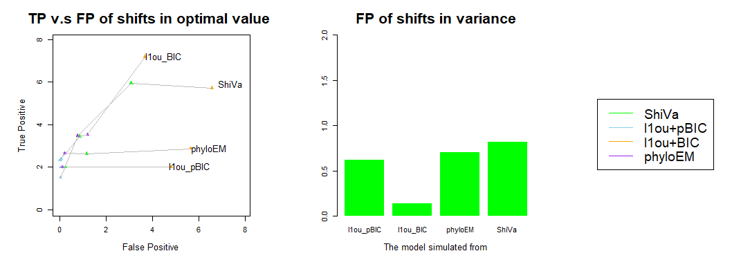
Figure 16: Left: True positive versus false positive rates of the shifts in optimal values detected by different methods. Right: False positive rates of the shifts in variance detected by ShiVa.

Figure 17: The selecting frequencies of shifts given by different methods; deeper color shows higher selecting frequency. (Green: selecting frequencies of shifts in optimal value; Red: selecting frequencies of shift in variance). The row names show the model data are simulated from; the column names show the method applied to the generated data. The asterisk marks show the true shifts of the model that the data are simulated from.

6 Conclusion

In this article, we have used a multi-optima multi-variance OU process to describe an evolutionary process where abrupt shifts can occur in either optimal value or variance. We then proposed a new method to simultaneously detect shifts in optimal value and shifts in variance. We implemented the method in R. Our package is available from the first author’s GitHub page https://github.com/WenshaZ/ShiVa. Furthermore, we have conducted simulation studies to show the effectiveness of our method to detect both kinds of shifts and compared it to methods which only detect shifts in optimal value.

We performed simulations of three different situations. When there are shifts in variance, our method has much lower false positive rate for shifts in mean than methods which do not model shifts in variance, since other methods wrongly detect the shift in variance as a large number of shifts in mean. As a result, our method has higher predictive log-likelihood than methods which do not model shifts in variance. When there are only shifts in optimal value, our method performs slightly worse than other methods when the number of shifts is large and the shift sizes are large. However, the gap between our method and the other methods is not substantial. Therefore, when shifts in variance exist, our method can effectively detect the true shifts or surrogates of the shifts in variance, leading to more accurate detection of shifts in optimal value and better predictive ability. And when there are no shifts in variance, our method has similar performance to other methods.

We applied our method to the first principal component of trait values for the cordylid data from Broeckhoven et al. (2016). ShiVa detected 7 shifts in optimal value and 3 shifts in variance and the model given by ShiVa has the highest log-likelihood and lowest BIC compared to $\ell$1ou and phyloEM. The validation result also shows Shiva would be unlikely to estimate the model it did if any of the models selected by other methods were true.

For model simplicity, we assume that the variance parameter is constant along each branch and that all shifts in variance happen at the beginning of the branch. Simulations of cases where these assumptions are violated show that our method is robust to misspecification in these assumptions. An interesting future research direction is to extend our model to allow shifts in variance at internal postions along a branch. This would allow us to estimate the exact time of a shift in variance. Writing the likelihood for this case is straightforward, but more work may be needed to ensure stability of the estimates. Another direction for future work is to improve the computational efficiency of the method. The likelihood calculation involves a large number of matrix inverse computations,which can be computationally expensive for large trees. Bastide et al. (2021) provide an efficient algorithm to calculate the log likelihood and its derivatives for certain phylogenetic models. If this method could be adapted to our method, it would lead to a major improvement in the computational speed, allowing our method to scale to larger phylogenies.

7 Data accessibility

The tree of Anolis lizards is provided by Mahler et al. (2013). The phylogenetic tree and principal component data of cordylid data ( Broeckhoven, Diedericks, Hui, Makhubo, and Mouton, 2016) are available in the R package phytools: http://www.phytools.org/Rbook/. Our R package is available at https://github.com/WenshaZ/ShiVa.

Appendices

A Supplemental figures

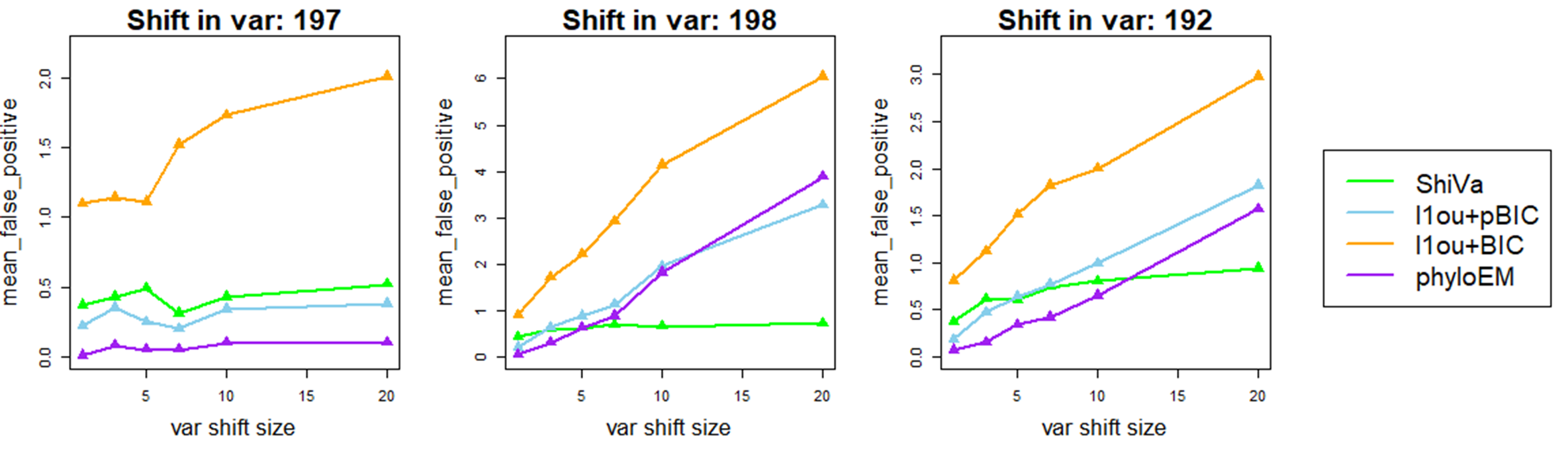
Figure 18: The false positive rates of different methods for detecting shifts in optimal value when there are only shifts in variance (Shift: 197; 198; 192)

Figure 19: The predictive log-likelihood difference of different methods when there are only shifts in variance (Shift: 197; 198; 192)

References

- Bastide et al. (2017) Paul Bastide, Mahendra Mariadassou, and Stéphane Robin. Detection of adaptive shifts on phylogenies by using shifted stochastic processes on a tree. Journal of the Royal Statistical Society: Series B (Statistical Methodology), 79(4):1067–1093, 2017. doi: 10.1111/rssb.12206.
- Bastide et al. (2021) Paul Bastide, Lam Si Tung Ho, Guy Baele, Philippe Lemey, and Marc A. Suchard. Efficient bayesian inference of general gaussian models on large phylogenetic trees. The Annals of Applied Statistics, 15(2), 2021. doi: 10.1214/20-aoas1419.
- Beaulieu et al. (2012) Jeremy M. Beaulieu, Dwueng-Chwuan Jhwueng, Carl Boettiger, and Brian C. O’Meara. Modeling stabilizing selection: Expanding the ornstein-uhlenbeck model of adaptive evolution. Evolution, 66(8):2369–2383, 2012. doi: 10.1111/j.1558-5646.2012.01619.x.
- Broeckhoven et al. (2016) Chris Broeckhoven, Genevieve Diedericks, Cang Hui, Buyisile G. Makhubo, and P. le Mouton. Enemy at the gates: Rapid defensive trait diversification in an adaptive radiation of lizards. Evolution, 70(11):2647–2656, 2016. doi: 10.1111/evo.13062.
- Butler and King (2004) Marguerite A. Butler and Aaron A. King. Phylogenetic comparative analysis: A modeling approach for adaptive evolution. The American Naturalist, 164(6):683–695, 2004. doi: 10.1086/426002.
- Felsenstein (1985) Joseph Felsenstein. Phylogenies and the comparative method. The American Naturalist, 125(1):1–15, 1985. doi: 10.1086/284325.
- Hansen (1997) Thomas F. Hansen. Stabilizing selection and the comparative analysis of adaptation. Evolution, 51(5):1341, 1997. doi: 10.2307/2411186.
- Ho and Ané (2013) Lam Si Tung Ho and Cécile Ané. Asymptotic theory with hierarchical autocorrelation: Ornstein–uhlenbeck tree models. The Annals of Statistics, 41(2), 2013. doi: 10.1214/13-aos1105.
- Ho and Ané (2014) Lam Si Tung Ho and Cécile Ané. Intrinsic inference difficulties for trait evolution with ornstein-uhlenbeck models. Methods in Ecology and Evolution, 5(11):1133–1146, 2014. doi: 10.1111/2041-210x.12285.
- Khabbazian et al. (2016) Mohammad Khabbazian, Ricardo Kriebel, Karl Rohe, and Cécile Ané. Fast and accurate detection of evolutionary shifts in ornstein–uhlenbeck models. Methods in Ecology and Evolution, 7(7):811–824, 2016. doi: 10.1111/2041-210x.12534.
- Losos (2011) Jonathan B. Losos. Lizards in an evolutionary tree: Ecology and adaptive radiation of anoles. University of California Press, 2011.
- Mahler et al. (2013) D. Luke Mahler, Travis Ingram, Liam J. Revell, and Jonathan B. Losos. Exceptional convergence on the macroevolutionary landscape in island lizard radiations. Science, 341(6143):292–295, 2013. doi: 10.1126/science.1232392.
- Mitov et al. (2020) Venelin Mitov, Krzysztof Bartoszek, Georgios Asimomitis, and Tanja Stadler. Fast likelihood calculation for multivariate gaussian phylogenetic models with shifts. Theoretical Population Biology, 131:66–78, 2020. doi: 10.1016/j.tpb.2019.11.005.
- Parikh (2014) Neal Parikh. Proximal algorithms. 2014. doi: 10.1561/9781601987174.
- Revell (2009) Liam J. Revell. Size-correction and principal components for interspecific comparative studies. Evolution, 63(12):3258–3268, 2009. doi: 10.1111/j.1558-5646.2009.00804.x.
- Stanley et al. (2011) Edward L. Stanley, Aaron M. Bauer, Todd R. Jackman, William R. Branch, and P. Le Mouton. Between a rock and a hard polytomy: Rapid radiation in the rupicolous girdled lizards (squamata: Cordylidae). Molecular Phylogenetics and Evolution, 58(1):53–70, 2011. doi: 10.1016/j.ympev.2010.08.024.
- Uyeda and Harmon (2014) Josef C. Uyeda and Luke J. Harmon. A novel bayesian method for inferring and interpreting the dynamics of adaptive landscapes from phylogenetic comparative data. Systematic Biology, 63(6):902–918, 2014. doi: 10.1093/sysbio/syu057.
- Zhang and Siegmund (2006) Nancy R. Zhang and David O. Siegmund. A modified bayes information criterion with applications to the analysis of comparative genomic hybridization data. Biometrics, 63(1):22–32, 2006. doi: 10.1111/j.1541-0420.2006.00662.x.
- Zhang et al. (2022) Wensha Zhang, Toby Kenney, and Lam Si Tung Ho. Evolutionary shift detection with ensemble variable selection, 2022. URL https://arxiv.org/abs/2204.06032.