Solving Decision-Dependent Games by Learning from Feedback

Abstract

This paper tackles the problem of solving stochastic optimization problems with a decision-dependent distribution in the setting of stochastic monotone games and when the distributional dependence is unknown. A two-stage approach is proposed, which initially involves estimating the distributional dependence on decision variables, and subsequently optimizing over the estimated distributional map. The paper presents guarantees for the approximation of the cost of each agent. Furthermore, a stochastic gradient-based algorithm is developed and analyzed for finding the Nash equilibrium in a distributed fashion. Numerical simulations are provided for a novel electric vehicle charging market formulation using real-world data.

Optimization, Stochastic monotone games, Decision-dependent distribution, Learning.

1 INTRODUCTION

The efficacy of stochastic optimization [1] and stochastic games [2, 3, 4, 5, 6] generally hinges on the premise that underlying data distribution is stationary. This means that the distribution of the data, which parametrize the problem or the game, does not change throughout the execution of the algorithm used to solve the stochastic problem or game, and is neither influenced or dependent on time nor the optimization variables themselves. This is a common setup that has been considered when game-theoretic frameworks have been applied to problems in, for example, ride hailing [7], routing [8], charging of electric vehicles (EVs) [9, 10], power markets [11], power systems [12], and in several approaches for training of neural networks [13]. However, this assumption can be invalid in a variety of setups in which the cost to be minimized is parameterized by data that is received from populations or a collection of automated control systems, whose response to is uncertain and depends on the output of the optimization problem itself. As an example, in a competitive market for electric EV charging [9, 14], the operators seek to find the charging prices (i.e., the optimization variables) to maximize the revenue from EVs; however, the expected demand (i.e., the “data” of the problem) is indeed dependent on the price itself. More broadly, power consumption in power distribution grids depends on electric prices [15]. A similar example pertains to ride hailing [7].

To accommodate this scenario, the so-called stochastic optimization with decision-dependent distributions (also known as performative prediction [16]) posits that we represent the data distribution used in optimization instead as a distributional map $x\mapsto D(x)$ where $x$ are decision variables [17, 18, 19, 16, 20]. In this work, we study decision-dependent stochastic games in which players seeks to minimize their cost (based on their optimization variables) subject to other players optimization variables, and where the data distribution of each player depends on the actions of all players (we will use the term player and agent interchangeably).

We focus on solving the Nash equilibrium problem of a game, which is to find a decision from which no agent is incentivized by their own cost to deviate when played. Formally, the stochastic Nash equilibrium problem with decision-dependent distributions considered in this paper is

$$x_{i}^{*}\in\operatorname*{arg\,min}_{x_{i}\in{\cal X}_{i}}F_{i}(x_{i},x_{-i}^{*}),\quad\forall\,i=1,\ldots,n$$ (1)

with $F_{i}(x_{i},x_{-i}^{*})$ defined as:

$$F_{i}(x_{i},x_{-i}^{*}):=\underset{z_{i}\sim D_{i}(x_{i},x_{-i}^{*})}{{\mathbb{E}}}f_{i}(x_{i},x_{-i}^{*},z_{i})$$ (2)

where: $z_{i}$ denotes a random variable supported on $\mathbb{R}^{k_{i}}$, $f_{i}:\mathbb{R}^{n}\times\mathbb{R}^{k_{i}}\rightarrow\mathbb{R}$ is a scalar valued function that is convex and continuously differentiable in $x_{i}$, ${\cal X}_{i}\subseteq\mathbb{R}$ is a convex set, and $D_{i}:\mathbb{R}^{n}\rightarrow{\cal P}(\mathbb{R}^{k_{i}})$ is a distributional map whose output is a finite-first moment Radon probability distribution supported on $\mathbb{R}^{k_{i}}$. Hence $x^{*}\in\mathbb{R}^{n}$, satisfies

$$F_{i}(x_{i}^{*},x_{-i}^{*})\leq F_{i}(x_{i},x_{-i}^{*})$$ (3)

for all $x_{i}\in{\cal X}_{i}$ and all $i=1,\ldots,n$.

Hereafter, we use the term “system” to refer to a population or a collection of automated controllers producing a response $z_{i}\in\mathbb{R}$ upon observing $x$. To illustrate, consider again the example where each agent represents an electric vehicle (EV) charging station service provider. Here, $x_{i}\in\mathbb{R}$ represents the charging price at a station managed by provider $i$, expressed in $/kWh. Correspondingly, $z_{i}$ indicates demand for the service at that price, while $f_{i}$ is the service cost (or the negative of the total profit) for provider $i$. This is an example of a competitive market in which the demand for service is a function of the price of all providers. EV owners react to price variations by choosing the service that aligns with their preferences (in terms of price and other externalities such as the locations of the charging stations).

The key challenge in problems of this form is that the distributional maps $D_{i}$ are often unknown [21, 22, 23, 24]. To overcome this challenge, we propose a two-stage optimization procedure – in the spirit of the methods proposed for convex optimization in [25, 18] – to tackle the multi-player decision-dependent stochastic game. The key idea behind this framework is that we first propose a parameterization for the distributional map in the system and estimate it from responses. Then, we use the estimated distributional map throughout the game without requiring further interaction with the system.

1.1 RELATED WORK

Our work incorporates themes from games, learning, as well as stochastic optimization with decision-dependent distributions. We highlight the relationship with this relevant literature below.

Games. Within the context of games, our work is specifically focused on solving Nash equilibrium problems using gradient-based methods and a variational inequality (VI) framework. The literature on stochastic games is extensive; for a comprehensive yet concise review of the subject, we refer the reader to the tutorials [26] and [2]; see also pertinent references therein. A common denominator of existing frameworks is that the data distribution is stationary. The work of [27] demonstrates that strictly monotone games have unique solutions and that gradient play converges to it. The modern approach of solving Nash equilibrium problems for continuous games via variational inequalities can be attributed to Facchinei and Pang [28, 29]. For solving strongly monotone variational inequalities, the projected gradient method is capable of converging linearly. However, merely monotone VI’s require extra gradient steps (Extragradient) or Tikhonov regularization [28]. The asymptotic convergence to the minimal norm solution was shown to be possible for decaying Tikhonov regularization parameters in [30].

Our work adds the additional complexity of minimizing communication between agents and hence we use a distributed gradient approach in our optimization algorithm. Distributed gradient methods have been explored extensively in the literature on convex optimization, though less so in that of variational inequalities. We refer the reader to [31] for a review in the convex optimization setting, and [32] for variational inequalities.

Decision-Dependent Data. This paper contributes to the growing body of literature that studies stochastic optimization with decision-dependent data distributions. While the concept of decision-dependence distributions has existed for some time, its roots go back to the framework “Performative Prediction” and its use within the machine learning community [16]; this work posits the formulation of optimization problems in which the data distribution is explicitly dependent on the optimization variables, and proposes repeated retraining (and the limit points thereof) as a solution. This is a family of points that solve the induced stationary optimization problem. For repeated retraining, convergence of various stochastic gradient algorithms are studied in [17, 33] in the batch setting, and in the time-varying setting in [34, 35]. The extension of problems with decision-dependent distributions to games includes two-player zero-sum games in [35], and general multiplayer games in [19].

Recent works have since pivoted towards directly solving the optimization problem by incorporating a model for the distributional map. In [18], the authors provide conditions that ensure convexity of the expected cost, alongside a two-stage algorithm for finding solutions of problems involving location scale-families. The work of [25] extends the two-stage algorithm to general distributional map-fitting problems and derives regret bounds that incorporate the associated approximation and statistical errors arising from the statistical learning problem. Outside of the two-stage approach, derivative-free methods have been studied in [18, 19, 20]. While these methods do not depend on a model of the distributional map, they generally exhibit slower convergence rates. On the other hand, adaptive learning strategies, particularly for location-scale models, have shown promise, as discussed in [19]. However, their exploration remains limited to this specific model category.

This work complements the technical findings in [25] by offering a generalization of the so called “Plug-in” approach of and by deriving error bounds under milder conditions. We also expand the findings of [19] by including the learning of the distributional maps.

1.2 CONTRIBUTIONS

In this work, we provide the following contributions to the body of work on stochastic optimization and Nash equilibrium problems with decision-dependent distributions.

• We propose a two-stage framework for stochastic optimization with decision-dependent data in the multi-player game settings. The first stage consists of an estimation of the distribution parameterization for each player. We show that the estimated cost for each player $F_{\widehat{\beta}_{i}}$ approximates the actual cost $F_{i}$, with an error that includes both an approximation component and a statistical estimation component:

  $$\|F_{\widehat{\beta}_{i}}-F_{i}\|_{\infty}\leq\texttt{Approximation}_{i}+\texttt{Estimation}_{i}.$$

• We further demonstrate sufficient conditions, which we call “Regular Problems”, for which the statistical estimation algorithm using $m$ samples satisfies

  $$\texttt{Estimation}_{i}=\mathcal{O}\left(\sqrt{\frac{\log m({d_{i}}+\log(1/\delta))}{m}}\right)$$

  with probability at least $1-\delta$, where $d_{i}$ is the number of parameters to be estimated. Our notion of regularity involves conditions that are easier to check relative to [25]. Additionally, we provide conditions under which best-response parameterizations, defined as

  $$z_{i} \overset{d}{=}\operatorname*{arg\,min}_{y}\left[-\langle y,\Psi_{\beta_{i}}(x)\rangle+\frac{1}{2}\|y-\xi_{i}\|^{2}\right]$$

  satisfy the regularity condition (symbols will be appropriately defined shortly in the paper).

• We develop a stochastic gradient-based algorithm for finding the Nash Equilibrium for monotone games, and we analyze its convergence for diffeent step size rules.

• Finally, we provide numerical simulations of an EV charging market formulation using real-world data. The EV market formulation is new in the context of energy markets, thus providing contributions in this area.

1.3 NOTATION

For $x,y\in\mathbb{R}^{n}$, we let $\langle x,y\rangle$ denote the inner product. For a given column vector $x\in\mathbb{R}^{n}$, $\|x\|$ is the Euclidean norm; for a matrix $X\in\mathbb{R}^{n\times m}$, $\|X\|_{F}$ denotes the Frobenious norm and $\|X\|_{\star}$ the nuclear norm. When random variables $X,Y\in\mathbb{R}^{k}$ are equal in distribution, $P(X\leq x)=P(Y\leq x)$ for all $x\in\mathbb{R}^{k}$, we write $X\overset{d}{=}Y$. For a given integer $n$, $[n]$ denotes the set $\{1,2,\ldots,n\}$.

1.4 ORGANIZATION

In Section 2, we discuss the proposed two-stage algorithm in detail and present our primary result. Section 3 discusses the details of the optimization stage. We provide our numerical simulations in Section 4. Proofs pf the results are provided in the Appendix.

2 Learning-based Decision-Dependent Games

In this work, we aim to solve the stochastic Nash equilibrium problem with decision dependent data distributions as formulated in (1). Regarding (1), we recall the following assumption, which will be used throughout the paper.

Assumption 1.

The function $x_{i}\mapsto f_{i}(x_{i},x_{-i},z_{i})$ is convex and continuously differentiable in $x_{i}$, for any fixed $x_{-i}$ and $z_{i}$. The set ${\cal X}_{i}\subseteq\mathbb{R}$ is convex.

In the following, we are interested in developing an algorithm capable of solving problems of this form, for well-behaved cost functions $f_{i}$ and distributional maps $D_{i}$, while minimizing the need for collaboration between players.

Methods for finding Nash equilibrium for games with decision dependent data distributions either use derivative free optimization, at the expense of an extremely slow rate, or use derivative information in conjunction with a model of the distributional map. The latter is due to the observation that $\nabla_{i}F_{i}$ requires that we compute the gradient of the probability distribution function of $z_{i}$ with respect to $x$. Indeed, $F_{i}$ can be written as

$$F_{i}(x)=\int_{\mathbb{R}^{k_{i}}}f_{i}(x,z_{i})p_{i}(z_{i};x)dz_{i},$$ (4)

where $z_{i}\mapsto p_{i}(z_{i},;x)$ is the probability density function corresponding to the probability distribution $D_{i}(x)$, and hence computing the gradient requires that we respect the product rule. This results in the gradient being given by

$$\nabla_{i}F_{i}(x)=\underset{z_{i}\sim D_{i}(x)}{{\mathbb{E}}}\left[\nabla_{x_{i}}f_{i}(x,z_{i})+f_{i}(x,z_{i})\nabla_{i}\log p_{i}(x;z_{i})\right].$$ (5)

To proceed, many works have observed that when $D_{i}$ takes the convenient form of a location-scale family and $f_{i}$ is convex in $x_{i}$, the objective retains convexity in $x_{i}$ and $\nabla_{i}F_{i}$ becomes tractable [18, 19]. In [25], it is shown that an “estimate-then-optimize” approach yields a bounded excess risk for the convex optimization problem with decision-dependent data. In this work, we seek to generalize such an approach to stochastic monotone games with decision-dependent data.

In this procedure, we require that each player estimates the distributional map $D_{i}$ from samples by proposing a hypothesis class of parameterized functions

$${\cal H}_{{\cal B}_{i}}=\left\{D_{\beta_{i}}|\ \beta_{i}\in{\cal B}_{i}\subseteq\mathbb{R}^{d_{i}}\right\},$$ (6)

as well as a suitable criterion or risk function $R_{i}$, to formulate an expected risk minimization problem

$$\beta^{*}_{i}\in\operatorname*{arg\,min}_{\beta_{i}\in{\cal B}_{i}}\underset{x\sim D_{i},\\ z_{i}\sim D_{i}(x)}{{\mathbb{E}}}R_{i}(x,z_{i},\beta_{i}).$$ (7)

In practice, we will estimate the expected risk from samples and solve the resulting empirical risk minimization (ERM) problem. To this end, we require that players collaborate by each deploying a set of decisions $\{x_{i}^{(j)}\}_{j=1}^{m}\overset{i.i.d}{\sim}D_{i}$ so that they can collectively receive feedback $z_{i}^{(j)}\sim D_{i}(x^{(j)})$ from the system (in response to their deployed decisions $\{x_{i}^{(j)}\}_{j=1}^{m}$). Then, based on the data $\{x^{(j)},z_{i}^{(j)}\}_{j=1}^{m}$, each player solves the following ERM problem

$$\widehat{\beta}_{i}\in\operatorname*{arg\,min}_{\beta_{i}\in{\cal B}_{i}}\frac{1}{m}\sum_{j=1}^{m}R_{i}(x^{(j)},z_{i}^{(j)},\beta_{i}).$$ (8)

The result is a distributional map $D_{\widehat{\beta}_{i}}$ approximating $D_{i}$, which we can now use to solve the approximate Nash equilibrium problem:

$$\widehat{x}_{i}\in\operatorname*{arg\,min}_{x_{i}\in{\cal X}_{i}}\left\{F_{\widehat{\beta}_{i}}(x_{i},\widehat{x}_{-i})\right\}$$ (9)

where

$$F_{\widehat{\beta}_{i}}(x_{i},\widehat{x}_{-i}):=\underset{z_{i}\sim D_{\widehat{\beta}_{i}}(x_{i},\widehat{x}_{-i})}{{\mathbb{E}}}f_{i}(x_{i},\widehat{x}_{-i},z_{i})\,.$$ (10)

By solving (9) instead of (1) we have introduced two forms of error: (i) approximation error of the distributional map $D_{i}$ by elements of the hypothesis class ${\cal H}_{i}$, and (ii) estimation or statistical error by solving the ERM problem instead of the expected risk minimization problem. In [25], the main result demonstrates that these two sources of error propagate through the optimization problem, and that the resulting excess risk can be bounded in terms of the sample complexity $m$. Our goal is to expand this result and provide additional analysis to our setting.

2.1 Parameter Estimation for Regular Problems

A critical component of our analysis is the estimation of the distributional map and the subsequent characterization of the estimation error. In this section, we outline a class of expected risk minimization problems, which we call regular problems, for which we can characterize the distance between expected risk minimization solutions and empirical risk minimization solutions. Throughout, we write $R_{i}(\beta_{i})={\mathbb{E}}_{(x,z)}[R(x,z_{i},\beta_{i})]$ and $\widehat{R}_{i}(\beta_{i})=(1/m)\sum_{j=1}^{m}R_{i}(x^{(j)},z_{i}^{(j)},\beta_{i})$ for $\beta_{i}\in\mathbb{R}^{d_{i}}$ to denote the expected and empirical risk, respectively.

Definition 1.

(Map Fitting Regularity) A map fitting problem, consisting of the optimization problems of $R_{i}$ and $\widehat{R}_{i}$ over ${\cal B}_{i}$, is regular provided that

1. Convexity: The expected risk $\beta\mapsto R_{i}(\beta)$ is $\mu_{i}$-strongly convex, and the empirical risk $\beta_{i}\mapsto\widehat{R}_{i}(\beta_{i})$ is convex.

2. Smoothness: For all realizations of $x\in{\cal X}$ and $z_{i}\in\mathbb{R}^{k_{i}}$, $\beta_{i}\mapsto\nabla_{\beta_{i}}R_{i}(x,z_{i},\beta_{i})$ is $L_{\beta_{i}}$-Lipschitz continuous.

3. Boundedness: The set ${\cal B}_{i}\subseteq\mathbb{R}^{d_{i}}$ is completely contained within a ball of radius $r_{i}$.

4. Sub-Exponential gradient: For all $\beta_{i}\in{\cal B}_{i}$, $\nabla_{\beta}R_{i}(x,z_{i},\beta_{i})$ is a sub-exponential vector with parameter $\nu_{i}>0$. $\Box$

Strong convexity guarantees uniqueness of $\beta_{i}^{*}$, and when combined with smoothness we have sufficient conditions for sub-linearly convergent algorithms that will find $\widehat{\beta}_{i}$. Lastly, the heavy-tail assumption [36] will allow us to describe the concentration of the gradient estimates. Together, they allow us to relate the solutions to the sample complexity in the following lemma.

Lemma 1.

(Uniform Gradient Bound) If the smoothness and sub-exponential gradient assumptions in Definition 1 hold for player $i\in[n]$, then for any $\delta\in(0,1/2)$ and any $m$ such that $m/\log(m)\geq 2(d_{i}+\log(1/\delta))$ we have that

$$\sup_{\beta\in{\cal B}}\|\nabla\widehat{R}_{i}(\beta)-\nabla R_{i}(\beta)\|\leq C_{i}\sqrt{\frac{\log(m)(d_{i}+\log(1/\delta))}{m}}$$ (11)

with probability at least $1-\delta$, where $C_{i}=4\max\{L_{\beta_{i}}/15r_{i},\nu_{i}\}$. $\Box$

The proof of this result is provided in the Appendix 5.1. This result offers a broad generalization of [37, Equation 19b] to any risk with Lipschitz continuous sub-exponential gradients over any convex and compact set. Our result is comparable to the $\mathcal{O}(\sqrt{d}{m})$ rate that can be found for specific problem instances such as linear least squares regression and logistic regression, but with the addition of a $\sqrt{\log m}$ factor. Indeed the generality of the risk function requires that we enforce compactness of the domain, thus giving rise to this extra logarithmic factor. This gradient estimation result will now allow us to reach our desired bounded distance result, which we present in the following theorem.

Theorem 2.

(ERM Approximation) If the map fitting problem is regular for player $i\in[n]$ (i.e., it satisfies the assumptions in Definition 1), then for any $\delta\in(0,1/2)$ and any $m$ such that $m/\log(m)\geq 2(d_{i}+\log(1/\delta))$ we have that

$$\|\widehat{\beta}_{i}-\beta_{i}^{*}\|\leq C_{i}^{\prime}\sqrt{\frac{\log(m)(d_{i}+\log(1/\delta))}{m}}$$ (12)

with probability at least $1-\delta$, where $C_{i}^{\prime}=(4/\mu_{i})\max\{L_{\beta_{i}}/15r_{i},\nu_{i}\}$. $\Box$

The proof of Theorem 2 is provided in the Appendix 5.2. The power in this characterization lies in the fact that it holds for any statistical learning problem satisfying the assumptions listed in Definition 1, and is not specific to the setting of learning distributional maps. We note that our Definition 1, which is a property used in the Theorem 2, is different from the one in [25] and it involves conditions that are easier to check.

As an example, we provide conditions for which a linear least squares problem satisfies the regularity conditions and hence is subject to the above ERM approximation result.

Proposition 3.

(Linear Least Squares Regularity) Consider the linear least squares problem with expected risk problem

$$B_{i}^{*}\in\operatorname*{arg\,min}_{B\in{\cal B}_{i}}\frac{1}{2}{\mathbb{E}}_{(x,z)}\|Bx-z\|^{2},$$

and empirical risk minimization problem

$$\widehat{B}_{i}\in\operatorname*{arg\,min}_{B\in{\cal B}_{i}}\frac{1}{2m}\sum_{j=1}^{m}\|Bx_{i}^{(j)}-{z_{i}^{(j)}}\|^{2}.$$

Let $x_{i}\sim D_{i}$ with zero mean and covariance matrix $\Sigma$. If
(i) There exist $\gamma_{i},L_{i}>0$ such that $\gamma_{i}I\leq\Sigma_{i}\leq L_{i}I$,
(ii) The entries of $xx^{T}$ and $zx^{T}$ are sub-exponential,
(ii) The constraint set ${\cal B}$ is convex and compact.
Then, the map fitting problem is regular. $\Box$

The proof of Proposition 3 is provided in Appendix 5.3. Deriving conditions for the more general case of non-linear regression is attainable but outside the scope of this work. We present a sufficient set of conditions for the regularity to hold.

Proposition 4.

(Nonlinear Regression) Consider the regularized non-linear least squares problem with expected risk problem

$$\beta^{*}_{i}\in\operatorname*{arg\,min}_{\beta\in{\cal B}_{i}}\frac{1}{2}{\mathbb{E}}_{(x,z)}\|\Psi_{\beta_{i}}(x)-z\|^{2}+\mu\|\beta\|^{2},$$ (13)

and empirical risk minimization problem

$$\widehat{\beta_{i}}\in\operatorname*{arg\,min}_{\beta\in{\cal B}_{i}}\frac{1}{2m}\sum_{j=1}^{m}\|\Psi_{\beta}(x_{i}^{(j)})-z_{i}^{(j)}\|^{2}+\mu\|\beta\|^{2}.$$ (14)

Suppose that
(i) the function $\beta_{i}\mapsto\|\Psi_{\beta_{i}}(x)-z\|^{2}$ is convex for fixed $(x,z)\sim(D_{i},D_{i}(x))$,
(ii) $\nabla\Psi_{\beta_{i}}(x)(\Psi_{\beta_{i}}(x)-z)$ is Lipschitz continuous in $\beta_{i}$, and sub-exponential for all $\beta_{i}$, and
(iii) the constraint set ${\cal B}_{i}$ is convex and compact.
Then, the map fitting problem is regular. $\Box$

2.2 Bounding the Approximation Error

Finding a relationship between $\widehat{x}$ and $x^{*}$ will require that we first characterize what constitutes an appropriate hypothesis class of distributions. Here, we formalize the notion of misspefication and sensitivity for a hypothesis class ${\cal H}_{{\cal B}_{i}}$.

Definition 2.

(Misspecification [25]) A hypothesis class ${\cal H}_{{\cal B}_{i}}$ is $\gamma_{i}$-misspecified provided that there exists a is $\gamma_{i}>0$ such that

$$W_{1}(D_{\beta_{i}^{*}}(x),D_{i}(x))\leq\gamma_{i}$$ (15)

for all $x\in{\cal X}$. $\Box$

This definition amounts to the distance between the function $D_{i}$ and the hypothesis class ${\cal H}_{{\cal B}_{i}}$ being close in the $W_{1}$ sense. Indeed if $\gamma_{i}=0$, then our approximation error is zero and we incur no bias in our problem formulation. Though, small values of $\gamma_{i}$ are appropriate as $D_{i}$ may be complex enough that approximating it with a finite-dimensional parameter space is difficult.

Definition 3.

(Sensitivity [25]) The hypothesis class ${\cal H}_{{\cal B}_{i}}$ is $\varepsilon_{i}$-sensitive if, for any $\beta_{i},\beta_{i}^{\prime}\in{\cal B}_{i}$,

$$W_{1}(D_{\beta_{i}}(x),D_{\beta_{i}^{\prime}}(x))\leq\varepsilon_{i}\|\beta_{i}-\beta_{i}^{\prime}\|$$ (16)

for all $x\in{\cal X}$. $\Box$

Sensitivity of ${\cal H}_{{\cal B}_{i}}$ is merely a convenient name for the condition that $\beta\mapsto D_{\beta_{i}}(x)$ be $\varepsilon_{i}$-lipschitz continuous for all realizations of $x\in{\cal X}$. In the result that follows, we demonstrate that an appropriately misspecified and sensitive hypothesis class and

Theorem 5.

(Bounded Approximation) Suppose that that the following conditions hold for any $i\in[n]$:
(i) The hypothesis class ${\cal H}_{{\cal B}_{i}}$ is $\gamma_{i}$-misspecified, and $\varepsilon_{i}$-sensitive.
(ii) The map fitting problem is regular.
(iii) For all $x\in{\cal X}_{i}$, $z_{i}\mapsto f_{i}(x,z_{i})$ is $L_{z_{i}}$-Lipschitz continuous.
Then, the bound

$$|F_{\widehat{\beta}_{i}}(x)-F_{i}(x)|\leq\gamma_{i}L_{z_{i}}+L_{z_{i}}\varepsilon_{i}C_{i}^{\prime}\zeta_{i}(m,\delta),$$ (17)

holds with probability $1-\delta$ for any $x\in{\cal X}_{i}$, where

$$\zeta_{i}(m,\delta):=\sqrt{\frac{\log(m)(d_{i}+\log(1/\delta))}{m}}\,.$$ (18)

Suppose that, additionally, the sets ${\cal X}_{i}$, $i\in[n]$, are compact and the function $x_{-i}\to F_{\beta_{i}}(x_{i},x_{-i})$ is $L^{\beta}_{-i}$-Lipschitz on ${\cal X}_{-i}$ for any $x_{i}\in{\cal X}_{i}$. Then,

$$|F_{i}(\widehat{x})-F_{i}(x^{*})|\leq ~{}2\gamma_{i}L_{z_{i}}+2L_{z_{i}}\varepsilon_{i}C_{i}^{\prime}\zeta_{i}(m,\delta)$$

$$+2\sqrt{2}\bar{L}_{i}\mathsf{diam}({\cal X})$$ (19)

hold with probability $1-\delta$ for any $\widehat{x}\in\widehat{{\cal X}}$ and $x^{*}\in{\cal X}^{*}$, where $\widehat{{\cal X}}$ and ${\cal X}^{*}$ are the sets of equilibria for (9) and (1), respectively, and $\bar{L}_{i}:=\max\{L_{i}^{\beta^{*}},L_{-i}^{\beta^{*}},L_{i}^{\widehat{\beta}},L_{-i}^{\widehat{\beta}}\}$. $\Box$

The proof of the Theorem 5 is provided in the Appendix 5.4. The analysis in this section demonstrates that the excess risk incurred by applying the proposed two-stage algorithm is made up of both approximation and estimation errors – the latter of which decays with increasing number of samples. Furthermore, this bound exists independent of the conditioning of the Nash equilibrium problem we solve in the second stage. We note that (17) is similar to the result in [25], but it is grounded on a different definition of regular problem (see Definition 1); the bound (19) is unique to this paper.

In the section that follows, we provide a class of hypothesis classes that allows the approximated game to be monotone, and provide suitable algorithms for solving them with convergence guarantees.

3 Solving Monotone Decision-dependent Games

In the previous section, we make the assumption that the Nash equilibrium problems (1) and (9) can be readily solved in order to contextualize our result in Theorem 5. In the case of (1), we cannot enforce that the ground truth distributional map $D_{i}$ satisfy any kind of assumption to guarantee convexity of $F_{i}$; however this can be done when prescribing a hypothesis class ${\cal H}_{i}$ to formulate (9). Moving forward, we propose a model class that balances expressiveness with tractability. Specifically, this model aims to: (i) accurately capture the behavior of the system, (ii) lead to a regular expected risk problem, (iii) maintain the monotonicity in the decision-dependent game.

A common model assumption used throughout the literature is that of a best-response mechanism. This posits that members of the population interact with the learning agents by modifying their stationary data in an optimal way:

$$z_{i}\overset{d}{=}\operatorname*{arg\,min}_{y}\left[-u_{\beta_{i}}(x,y)+\frac{1}{2}\|y-\xi_{i}\|^{2}\right],$$

where $\xi_{i}\sim D_{i}$ is a stationary random variable associated with the $i$th agent; $u_{\beta_{i}}$ is a utility function parameterized by $\beta_{i}\in{\cal B}_{i}$ corresponding the utility that members of the population derive from changing their data in response to the decisions in $x$; and the quadratic term $1/2\|y-\xi_{i}\|^{2}$ is the cost of changing their data from $\xi$ to $y$. As a means of reconciling the above traits, this work will focus on best-response models with a linear-composite utility, $u_{\beta_{i}}(x,y)=\langle y,\Psi_{\beta_{i}}(x)\rangle$, for some function $\Psi_{\beta_{i}}$ that is appropriate for the problem.

Substituting into the above problem yields

$$z_{i} \overset{d}{=}\operatorname*{arg\,min}_{y}\left[-\langle y,\Psi_{\beta_{i}}(x)\rangle+\frac{1}{2}\|y-\xi_{i}\|^{2}\right]$$

$$\overset{d}{=}\Psi_{\beta_{i}}(x)+\xi_{i}.$$

Hence the minimization problem can be solved uniquely, and the resulting model can be simply expressed as the sum of stationary data and a decision-dependent perturbation. Since this is a non-linear model in general, we can simply apply non-linear regression to learn the parameter $\beta_{i}$ from samples:

$$\widehat{\beta}_{i}=\operatorname*{arg\,min}_{\beta_{i}}\frac{1}{2m}\sum_{j=1}^{m}\|z_{i}^{(j)}-\Psi_{\beta_{i}}(x^{(j)})\|^{2}+\mu\|\beta\|^{2}$$ (20)

where we include the Tikhonov regularization to favor tractability. Additionally, the resulting payoff function $F_{\beta_{i}}$ has gradient $\nabla_{i}F_{\beta_{i}}(x)={\mathbb{E}}_{z_{i}\sim D_{i}(x)}\left[\nabla_{i}f_{i}(x,z)+\nabla_{i}\Psi_{\beta_{i}}(x)^{T}\nabla_{z_{i}}f_{i}(x,z)\right]$, for which the distributional component $\nabla_{i}f_{i}(x,z)+\nabla_{i}\Psi_{\beta_{i}}(x)^{T}\nabla_{z_{i}}f_{i}(x,z)$ has nice properties when $\nabla_{i}\Psi_{\beta_{i}}$ is simple to analyze. In what follows, we show that best-response models of this form satisfy the sensitivity condition, thus making them suitable for further analysis.

Proposition 6.

(Best-response Smoothness) Consider the class of linear best-response models given by

$${\cal H}_{{\cal B}_{i}}=\left\{D_{\beta_{i}}\bigg{|}\ \ z_{i}\overset{d}{=}\xi_{i}+\Psi_{\beta_{i}}(x)\sim D_{\beta_{i}}(x),\ \forall x\ \right\}$$ (21)

having parameter function $\Psi_{\beta_{i}}:\mathbb{R}^{n}\rightarrow\mathbb{R}$ and stationary random variables $\xi_{i}\sim D_{i}$. If $\beta_{i}\mapsto\Psi_{\beta_{i}}$ is $\varepsilon_{i}$-Lipschitz continuous for all $x\in{\cal X}$, then ${\cal H}_{{\cal B}_{i}}$ is $\varepsilon_{i}$-smooth. $\Box$

The proof of Proposition 6 is provided in the Appendix 5.5. Next, we proceed by providing a gradient-based algorithm for solving (merely) monotone games.

3.1 Regularized-Distributed Gradient Play

Now that the details of the estimation stage, and suitable model classes have been identified, we can address the second stage of the two stage algorithm. A crucial component of interest is allowing the gradient map of the game to be merely monotone, as opposed to the strong monotonicity requirement, while simultaneously preventing the need for collaborating between players. Typically, solving problems of this form using the Extragradient method achieves the ideal rate without perturbing the problem. A caveat of this approach however, is that it requires that every agent shares their gradient information with all other agents. In several realistic applications (such as energy markets or transactive setups), such collaboration is often impossible because it would involve sharing of private information.

Instead, we propose a Tikhnov regularization scheme in which each player can set their own regularization parameters and step-sizes, and provide conditions for which convergence can be achieved provided that each player meets them. At initialization, each player chooses a starting point $x_{i}^{0}$, a step size $\eta_{i}^{0}$, and a regularization parameter. The algorithm then proceeds by each player computing the iterates (with $k\in\mathbb{N}$ the iteration index):

$$x_{i}^{k+1}=\mathsf{Proj}_{{\cal X}_{i}}\left[x_{i}^{k}-\eta_{i}^{k}\left(G_{i}(x_{i}^{k})+\lambda_{i}x_{i}^{k}\right)\right],$$ (22)

where $G_{i}$ is a stochastic estimate of $\nabla_{i}F_{i}$, then reporting the result. We lay out a stochastic framework for our analysis.

Assumption 2.

(Stochastic Framework) Fix a probability space $({\cal S},{\cal F},\mathbb{P})$ with sample space ${\cal S}$, $\sigma$-algebra ${\cal F}$, and probability measure $\mathbb{P}$. For each $i\in[n]$, equip $\mathbb{R}^{k_{i}}$ with the Borel $\sigma$-algebra.

Let $\mathbb{F}=\{{\cal F}_{k}\}_{k\geq 0}$ be a filtration on $({\cal S},{\cal F},\mathbb{P})$ such that ${\cal F}_{0}=\{\emptyset,{\cal S}\}$, and $g_{i}^{k}$ is ${\cal F}_{k}$-measurable. The gradient map $G_{i}$ for each agent, and its corresponding stochastic estimator $g_{i}^{k}$ drawn at each iteration $k$ of the algorithm satisfy:

(Bias) $$\qquad\qquad\|{\mathbb{E}}_{k}g_{i}^{k}-G_{i}(x^{k})\|\leq\beta_{i}^{k}$$

(Variance) $$\qquad\qquad{\mathbb{E}}_{k}\|g_{i}^{k}-{\mathbb{E}}_{k}g_{i}^{k}\|^{2}\leq\sigma_{i}^{k}$$

for sequences $\{\beta_{i}^{k}\}_{k\geq 0},\{\sigma_{i}^{k}\}_{k\geq 0}\subseteq\mathbb{R}_{+}$. $\Box$

Considering this framework, we provide conditions for which a single step of our distributed gradient algorithm is practically contractive.

Theorem 7.

(Contractivity) Suppose that Assumptions 1-2 hold and consider the iteration (22). For each $i\in[n]$, we have that

$${\mathbb{E}}_{k}\|x_{i}^{k+1}-x_{i}^{*}\|^{2}\leq \frac{1}{1+\eta_{i}\lambda_{i}}\|x_{i}^{k}-x_{i}^{*}\|^{2}$$

$$+\frac{2\eta_{i}(\beta_{i}^{k})^{2}}{\lambda_{i}(1+\eta_{i}\lambda_{i})}+\frac{2\eta_{i}^{2}(\sigma_{i}^{k})^{2}}{1+\eta_{i}\lambda_{i}}$$ (23)

provided that $\eta_{i}\leq\lambda_{i}/(4L_{i}^{2})$. $\Box$

The proof of Theorem 7 is provided in the Appendix 5.6. Following this one-step analysis, we can show convergence with a decaying step-size policy.

Corollary 8.

(Sub-linear Convergence) Under the same assumptions of Theorem 7, suppose that

$$\beta_{i}^{k}\leq\frac{\beta_{i}}{\sqrt{\omega_{i}+k}},\ \text{and}\ \eta_{k}=\frac{2}{\lambda_{i}^{2}(\gamma_{i}+k-2)}.$$

Then the iterates of (22) satisfy

$${\mathbb{E}}_{k}\|x_{i}^{k+1}-x_{i}^{*}\|^{2}\leq\frac{\xi}{\lambda_{i}^{2}(\gamma_{i}+k)},$$

where $\xi:=\max\left\{\gamma_{i}\lambda_{i}^{2}\|x_{i}^{0}-x_{i}^{*}\|^{2},2\beta_{i}^{2}\theta+4\Delta\varphi\right\}$. $\Box$

Proof of this result follows by a standard induction argument.

4 Numerical Experiments on Electric Vehicle Charging

In this section, we consider a competitive game between $n$ distinct electric vehicle charging station operators, where stations are equipped with renewable power sources. The goal of each player is to set prices to maximize their own profit in a system where demand for their station will change in response to the prices set by other competing stations as well. The cost function (negative profit) takes the form

$$f_{i}(x,z_{i})=-\left[\underbrace{z_{i}x_{i}}_{\text{service profit}}+\underbrace{p_{w}\phi(w_{i}-z_{i})}_{\text{renewable profit}}-\underbrace{p_{r}\phi(z_{i}-w_{i})}_{\text{operational cost}}\right]$$

where $\phi(y)=\log(1+\exp(y))$ for all $y\in\mathbb{R}$. The renewable profit and operational cost terms allow us to describe the trade-off between profit from renewable power generation sold to the grid at rate $p_{w}$, and surplus power required from the grid to meet demand at rate $p_{r}$. To find an optimal price, we can formulate a Nash equilibrium problem over the expected cost $F_{i}(x)={\mathbb{E}}_{z_{i}\sim D_{i}(x)}[f_{i}(x,z_{i})]$ for $x\in{\cal X}=\Pi_{i=1}^{n}{\cal X}_{i}$ where ${\cal X}_{i}=[p_{w},p_{r}]$ is the interval of price values between the wholesale price and retail.

Since the set of reasonable prices will be quite small, we hypothesize that the the price and demand have a linear relationship of the form $z_{i}\overset{d}{=}\xi_{i}+\beta_{i}x_{i}+\langle\beta_{-i},x_{-i}\rangle$ where $\beta_{i}\in\mathbb{R}$ and $\beta_{-i}\in\mathbb{R}^{n-1}$. Since we have a simple model, the first and second derivatives can be computed in closed form, and shown to be positive definite provided that $\beta_{i}>0$

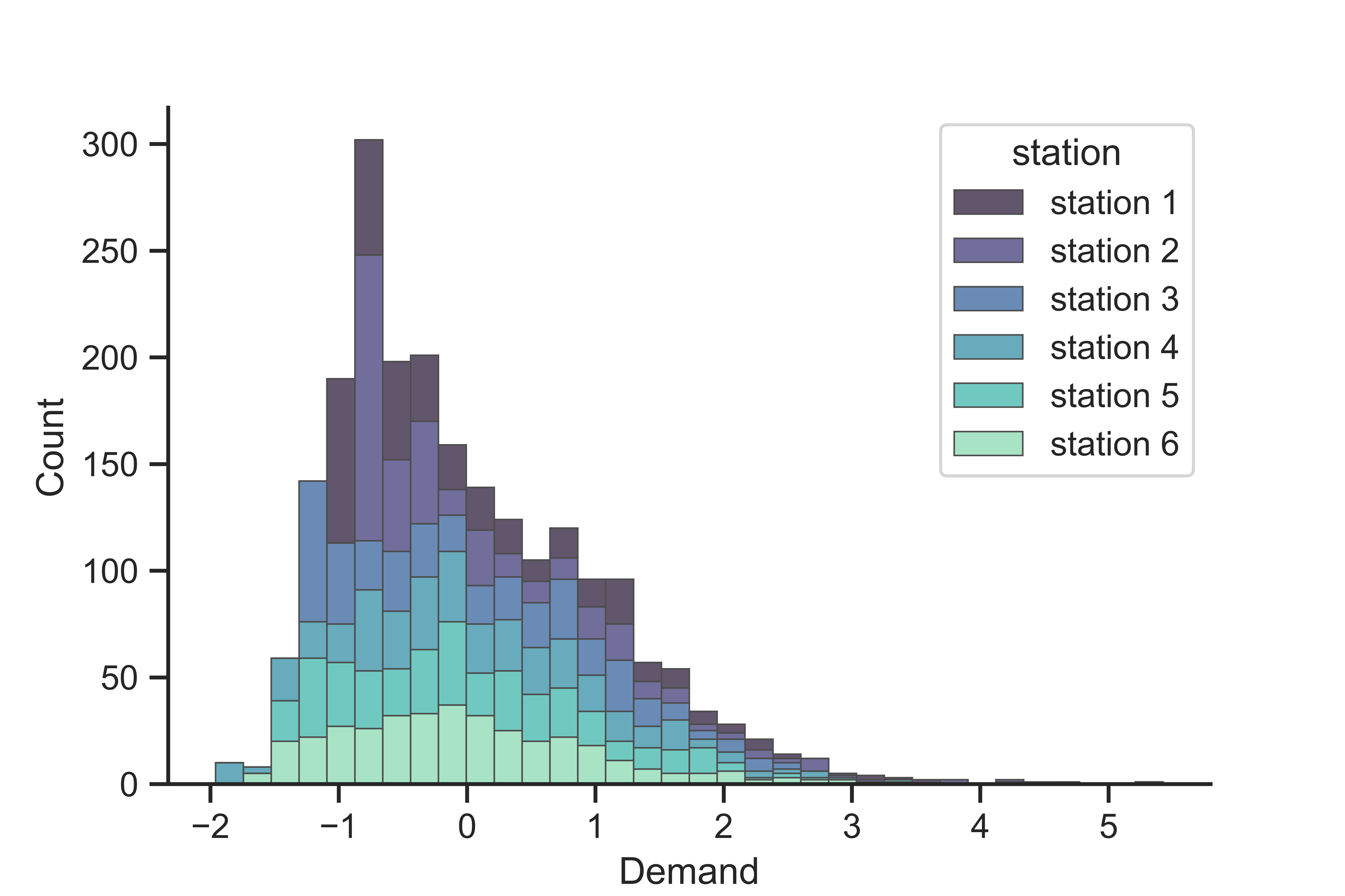
Figure 1: Standardized demand data for six medium demand EVCS’s with either consisting of either 2 or 6 ports and port power values of 50, 150, and 350 kWh. Standardization maps raw demand instances to instances of demand that are deviations from the average at each station.

Our data depicts the demand of electricity across an hour-long period for 6 ports of varying power profiles for each day in year. We standardize the data to be zero mean and unit variance across each station. The cost of each agent is regularized with $\lambda=1.0$. Solutions are calculated by performing expected gradient play with constant step size; the expected mean is estimated via the empirical mean over the data set.

To demonstrate the impact of the decision-dependence on the problem we use two distinct elasticity profiles for the problem. We set $\beta$ We set $\beta_{i}=-\beta$ and $\beta_{-i}=\beta\mathds{1}$ for $\beta\in\{0.1,0.3\}$. Hence demand for agent $i$ decreases as their own price increases, and increases as the price of other agents decreases. We run the stochastic gradient play algorithm with a single sample at each round and a decaying step size policy $\eta_{k}=c/(1+k)$ for appropriately chosen constant c. We find that the linear model lends gives rise to faster convergence with lower error in the same number of iterations.

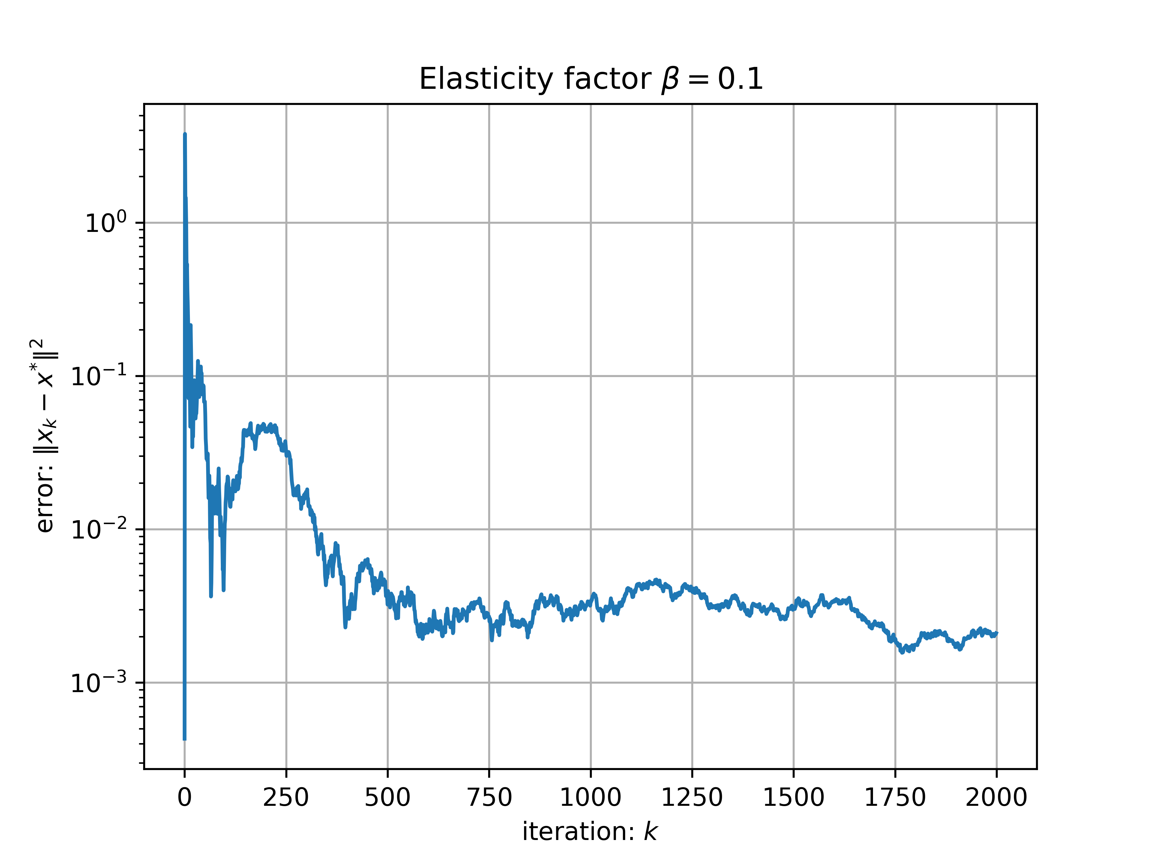
Figure 2: Regularized stochastic gradient descent with decaying step size for a linear best response model with elasticity factor $\beta=0.1$

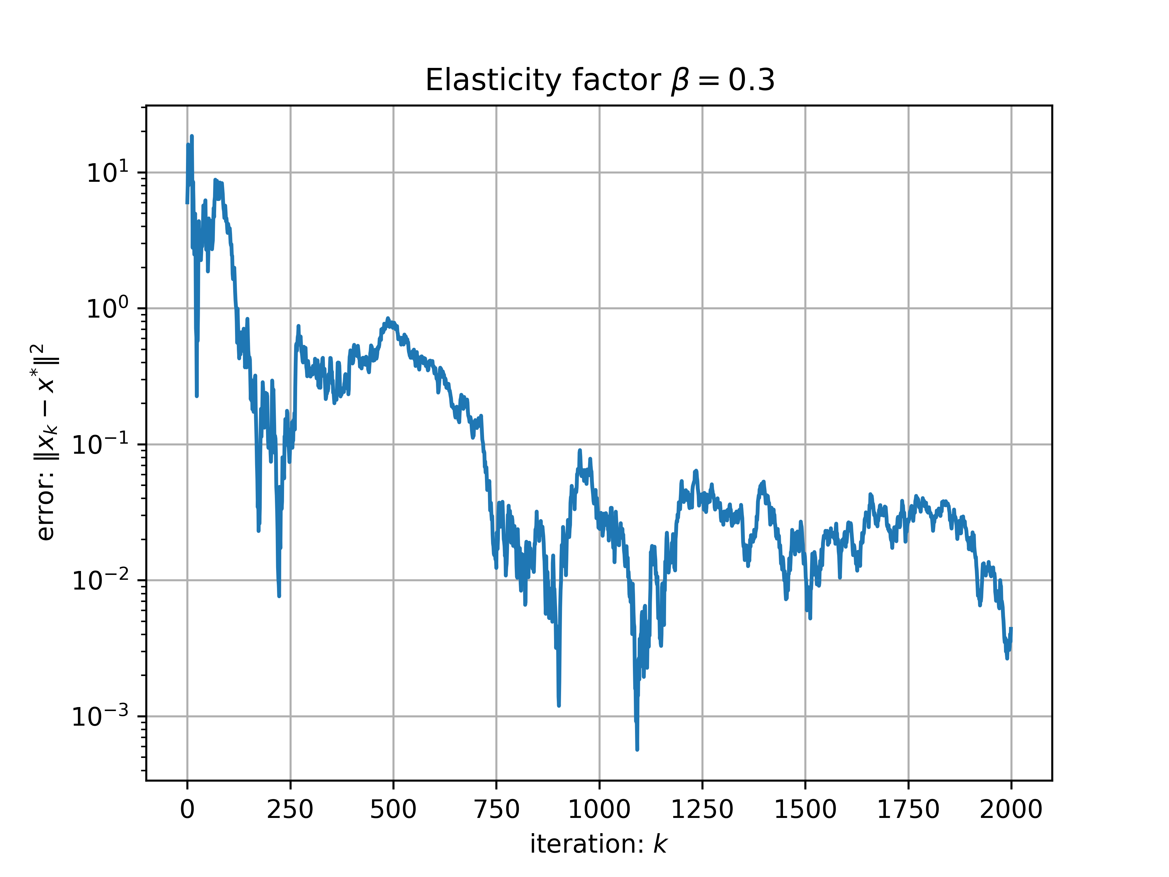
Figure 3: Regularized stochastic gradient descent with decaying step size for a linear best response model with elasticity factor $\beta=0.3$

5 CONCLUSIONS

In this work, we studied a class of stochastic Nash equilibrium problems, characterized by data distributions that are dependant on the decisions of all involved players. We showed that an ’estimate-then-optimize’ approach enables the formulation of an Nash equilibrium problem that is solvable either using classical methods when collaboration is feasible, or via a novel regularized distributed method in the absence of collaboration. In both instances, the results of this procedure is a payoff that can be related to payoff of the original Nash equilibrium problem via an error that depends on both our approximation and estimation error. To demonstrate the flexibility of these findings, we simulated these techniques in an electric vehicle charging market problem in which service providers set prices, and users modify their demand based on prices set by providers. Future research will look at a scenario where the estimate of the distributional map is improved during the operation of the algorithm, based on the feedback received.

APPENDIX

5.1 Proof of Lemma 1

For the sake of notation convenience, and visual clarity, we will suppress the $i$ index throughout the proof. We denote the gradient error by $\rho(\beta)=\nabla\widehat{R}(\beta)-\nabla R(\beta)$ for all $\beta\in\mathbb{R}^{d}$.

To begin, we will generate coverings for the unit sphere in $\mathbb{R}^{d}$ and ${\cal B}\subseteq\mathbb{R}^{d}$ and use a discretization argument to create bounds over these finite sets. Fix $\beta\in{\cal B}$ and $u\in{\cal S}^{d-1}$. Let $\{u_{j}\}_{j=1}^{N}$ be an arbitrary $1/2$-covering of the sphere $\mathbb{S}^{d_{\beta_{i}}}$ with respect to the Euclidean norm. From [38, Lemma 5.7], we know that $N\leq 5^{d}$. From our covering, we have that there exists $u_{j}$ in the covering such that $\|u-u_{j}\|\leq 1/2$. Hence,

$$\langle u,\rho(\beta)\rangle =\langle u_{j}+(u-u_{j}),\rho(\beta)\rangle$$

$$=\langle u_{j},\rho(\beta)\rangle+\langle u-u_{j},\rho(\beta)\rangle$$

$$\leq\langle u_{j},\rho(\beta)\rangle+\|u-u_{j}\|\|\rho(\beta)\|$$

$$\leq\langle u_{j},\rho(\beta)\rangle+\frac{1}{2}\|\rho(\beta)\|$$

$$\leq\max_{j\in[N]}\langle u_{j},\rho(\beta)\rangle+\frac{1}{2}\|\rho(\beta)\|\,.$$

Since this is true for any $u\in{\cal S}^{d-1}$, then it holds for $u=\rho(\beta)/\|\rho(\beta)\|$. Thus the above becomes

$$\|\rho(\beta)\|\leq 2\langle u_{j},\rho(\beta)\rangle\leq 2\max_{j\in[N]}\langle u_{j},\rho(\beta)\rangle.$$ (24)

Now we fix $\varepsilon\in(0,1]$, and choose and $\varepsilon$-covering for the set ${\cal B}$, which we will write as $\{\beta_{k}\}_{k=1}^{M}$. Recall that ${\cal B}$ is bounded, so there exists a constant $r>0$ such that for all $\beta\in{\cal B}$, $\|\beta\|\leq r$. Hence ${\cal B}\subseteq B(r)$. From [36, Proposition 4.2.12], we have that

$$M\leq\frac{\operatorname*{vol}\left(B(r)+\frac{\varepsilon}{2}B(1)\right)}{\operatorname*{vol}\left(\frac{\varepsilon}{2}B(1)\right)}=\frac{\operatorname*{vol}\left(\frac{3}{2}B(r)\right)}{\operatorname*{vol}\left(\frac{\varepsilon}{2}B(1)\right)}=\left(\frac{3r}{\varepsilon}\right)^{d}.$$ (25)

Thus, we conclude that $M\leq(3r/\varepsilon)^{d}$.

Now by our discretization argument, there exists $k\in[M]$ such that $\|\beta-\beta_{k}\|\leq\varepsilon$ and hence

$$\max_{j\in[N]}\langle u_{j},\rho(\beta)\rangle =\max_{j\in[N]}\langle u_{j},\rho(\beta_{k})+(\rho(\beta)-\rho(\beta_{k})\rangle$$

$$=\max_{j\in[N]}\langle u_{j},\rho(\beta_{k})\rangle+\langle u_{j},\rho(\beta)-\rho(\beta_{k})\rangle$$

$$\leq\max_{j\in[N]}\langle u_{j},\rho(\beta_{k})\rangle+\max_{j\in[N]}\langle u_{j},\rho(\beta)-\rho(\beta_{k})\rangle$$

$$\leq\max_{k\in[M]}\max_{j\in[N]}\langle u_{j},\rho(\beta_{k})\rangle$$

$$\ +\sup_{\|\alpha-\alpha^{\prime}\|\leq\varepsilon}\max_{j\in[N]}\langle u_{j},\rho(\alpha)-\rho(\alpha^{\prime})\rangle.$$

We observe that if $\alpha,\alpha^{\prime}\in{\cal B}$ are such that $\|\alpha-\alpha^{\prime}\|\leq\varepsilon$, then applying our smoothness assumption yields

$$\langle u_{j},\rho(\alpha)-\rho(\alpha^{\prime})\rangle$$

$$=\langle u_{j},(\nabla\widehat{R}(\alpha)-\nabla R(\alpha))-(\nabla\widehat{R}(\alpha^{\prime})-\nabla R(\alpha^{\prime}))\rangle$$

$$=\langle u_{j},\nabla\widehat{R}(\alpha)-\nabla\widehat{R}(\alpha^{\prime})\rangle+\langle u_{j},\nabla R(\alpha^{\prime})-\nabla R(\alpha)\rangle$$

$$\leq\|u_{j}\|\|\nabla\widehat{R}(\alpha)-\nabla\widehat{R}(\alpha^{\prime})\|+\|u_{j}\|\|\nabla R(\alpha)-\nabla R(\alpha^{\prime})\|$$

$$\leq L_{\beta_{i}}\|\alpha-\alpha^{\prime}\|+L_{\beta_{i}}\|\alpha-\alpha^{\prime}\|$$

$$\leq 2L_{\beta}\varepsilon,$$

where the second-to-last inequality uses $\|u_{j}\|=1$.

To bound the remaining term, we use the concentration of sub-exponential random variables, due to Bernstein’s Inequality combined with the Union Bound. We have that

$${\mathbb{P}}\left(\langle u_{j},\rho(\beta_{k})\rangle\geq t\right)\leq 2\exp\left(-\frac{mt^{2}}{2\nu^{2}}\right)$$

for all $t\leq\nu$, and hence

$${\mathbb{P}}\left(\max_{k\in[M]}\max_{j\in[N]}\langle u_{j},\rho(\beta_{k}\rangle\geq t\right)$$

$$={\mathbb{P}}\left(\bigcup_{k\in[M]}\bigcup_{j\in[N]}\{\langle u_{j},\rho(\beta_{k}\rangle\geq t\}\right)$$

$$\leq\sum_{k\in[M]}\sum_{j\in[N]}{\mathbb{P}}\left(\{\langle u_{j},\rho(\beta_{k}\rangle\geq t\}\right)$$

$$\leq\sum_{k\in[M]}\sum_{j\in[N]}2\exp\left(-\frac{mt^{2}}{2\nu^{2}}\right)$$

$$=M\cdot N\cdot 2\exp\left(-\frac{mt^{2}}{2\nu^{2}}\right)$$

$$\leq 2\left(\frac{15r}{\varepsilon}\right)^{d}\exp\left(-\frac{mt^{2}}{2\nu^{2}}\right)$$

for all $t\leq\nu$, where we used the fact that $M\leq(3r/\varepsilon)^{d}$ and $N\leq 5^{d}$. Setting the right hand side equal to $2\delta$ yields

$$t=\sqrt{2}\nu\sqrt{\frac{d\log(15r/\varepsilon)+\log(1/\delta)}{m}}.$$ (26)

Next we choose $\varepsilon=\frac{1}{15r}\sqrt{\frac{d+\log(1/\delta)}{m}}$ so that

$$t =\sqrt{2}\nu\sqrt{\frac{d\log(15r/\varepsilon)+\log(1/\delta)}{m}}$$

$$=\sqrt{2}\nu\sqrt{\frac{\frac{d}{2}\log(m)-\frac{d}{2}\log(d+\log(1/\delta))+\log(1/\delta)}{m}}$$

$$\leq\sqrt{2}\nu\sqrt{\frac{d\log(m)+\log(1/\delta)}{m}}$$

$$\leq\sqrt{2}\nu\sqrt{\frac{\log(m)(d+\log(1/\delta))}{m}}.$$

By requiring that $m$ satisfy $m/\log(m)\geq 2(d+\log(1/\delta))$, we enforce that $t\leq\nu$. In combining, we observe that

$$t+2\varepsilon L$$

$$\leq\sqrt{2}\nu\sqrt{\frac{\log(m)(d+\log(1/\delta))}{m}}+\frac{2L}{15r}\sqrt{\frac{d+\log(1/\delta)}{m}}$$

$$\leq 2\left(\nu+\frac{L}{15r}\right)\sqrt{\frac{\log(m)(d+\log(1/\delta))}{m}}$$

$$\leq 4\max\left\{\frac{L}{15r},\nu\right\}\sqrt{\frac{\log(m)(d+\log(1/\delta))}{m}},$$

and the result follows.

5.2 Proof of Theorem 2

We suppress the subscript $i$ for notational simplicity. We recall that that the $\mu$-strong convexity of the map $\beta\mapsto R(x,z;\beta)$ implies $\mu$-strong monotonicity of $\nabla R(\beta)$, and $\nabla\widehat{R}(\beta)$. It follows that

$$\mu\|\widehat{\beta}-\beta^{*}\|^{2} \leq\langle\widehat{\beta}-\beta^{*},\nabla R(\widehat{\beta})-\nabla R(\beta^{*})\rangle$$

$$=\langle\widehat{\beta}-\beta^{*},\nabla R(\widehat{\beta})\rangle-\langle\widehat{\beta}-\beta^{*},\nabla R(\beta^{*})\rangle$$

$$\leq\langle\widehat{\beta}-\beta^{*},\nabla R(\widehat{\beta})\rangle$$

$$\leq\langle\widehat{\beta}-\beta^{*},\nabla R(\widehat{\beta})\rangle+\langle\beta^{*}-\widehat{\beta},\nabla\widehat{R}(\widehat{\beta})\rangle$$

$$=\langle\widehat{\beta}-\beta^{*},\nabla R(\widehat{\beta})-\nabla\widehat{R}(\widehat{\beta})\rangle$$

$$\leq\|\widehat{\beta}-\beta^{*}\|\sup_{\beta\in{\cal B}}\|\nabla R(\beta)-\nabla\widehat{R}(\beta)\|$$

and hence

$$\|\widehat{\beta}-\beta^{*}\|\leq\frac{1}{\mu}\sup_{\beta\in{\cal B}}\|\nabla R(\beta)-\nabla\widehat{R}(\beta)\|.$$ (27)

The result now follows by applying Lemma 1.

5.3 Proof of Proposition 3

We suppress the $i$ index throughout. The associated risk function is $R(x,z,B)=\frac{1}{2}\|Bx-z\|^{2}$, so that $\nabla R(x,z,B)=(Bx-z)x^{T}=Bxx^{T}-zx^{T}$ and $\nabla^{2}R(x,z,B)=xx^{T}$ are the corresponding gradient and hessian. We observe that enforcing $\gamma I\leq{\mathbb{E}}[xx^{T}]\leq LI$ for some $\gamma,L>0$ ensures $\gamma$-strong convexity and $L$-smoothness of the expected risk. Similarly, the empirical risk has gradient $\nabla R_{m}(B)=1/m(BXX^{T}-ZX^{T})$, and hessian $\nabla^{2}R_{m}(B)=(1/m)XX^{T}$. Thus $R_{m}$ is convex the hessian is symmetric, then it is positive semi-definite and thus $R_{m}$ is convex. Furthermore, smoothness of $R_{m}$ follows with constant $\max\{L,\|XX^{T}\|_{2}\}$. Lastly, since $zx^{T}$ and $xx^{T}$ have sub-exponential entries, the gradient is sub-exponential and the result follows.

5.4 Proof of Theorem 5

We observe that for any fixed $x\in\mathcal{X}$, we have that $|F_{\widehat{\beta}_{i}}(x)-F_{i}(x)|\leq|F_{\widehat{\beta}_{i}}(x)-F_{\beta_{i}^{*}}(x)|+|F_{\beta_{i}^{*}}(x)-F_{i}(x)|$. The first term describes our statistical error at $x$. We denote $\Pi(D_{\widehat{\beta}_{i}},D_{\beta_{i}^{*}})$ as a coupling on ${\cal P}(\mathbb{R}^{m_{i}})$ so that

$$|F_{\widehat{\beta}_{i}}(x)-F_{\beta_{i}^{*}}(x)|$$

$$=\left|\inf_{\Pi(D_{\widehat{\beta}_{i}}(x),D_{\beta_{i}^{*}}(x))}\ {\mathbb{E}}_{(z,z^{\prime})\sim\Pi(D_{\widehat{\beta}_{i}}(x),D_{\beta_{i}^{*}}(x))}\left(f(x,z)-f(x,z^{\prime})\right)\right|$$

$$\leq\inf_{\Pi(D_{\widehat{\beta}_{i}}(x),D_{\beta_{i}^{*}}(x))}\ {\mathbb{E}}_{(z,z^{\prime})\sim\Pi(D_{\widehat{\beta}_{i}}(x),D_{\beta_{i}^{*}}(x))}\left|f(x,z)-f(x,z^{\prime})\right|$$

$$\leq L_{z_{i}}\left(\inf_{\Pi(D_{\widehat{\beta}_{i}}(x),D_{\beta_{i}^{*}}(x))}\ {\mathbb{E}}_{(z,z^{\prime})\sim\Pi(D_{\widehat{\beta_{i}}}(x),D_{\beta_{i}^{*}}(x))}\|z_{i}-z_{i}^{{}^{\prime}}\|\right)$$

$$=L_{z_{i}}W_{1}(D_{\widehat{\beta}_{i}}(x),D_{\beta_{i}^{*}}(x))$$

$$\leq L_{z_{i}}\varepsilon_{i}\|\widehat{\beta}_{i}-\beta_{i}^{*}\|\,.$$

By similar argument, we find that $|F_{\beta_{i}^{*}}(x)-F_{i}(x)|\leq L_{z_{i}}W_{1}(D_{\beta_{i}^{*}}(x),D_{i}(x))\leq L_{z_{i}}\gamma_{i}$. In combining, we get $|F_{\widehat{\beta}_{i}}(x)-F_{i}(x)|\leq L_{z_{i}}\varepsilon_{i}\|\widehat{\beta}_{i}-\beta_{i}^{*}\|+L_{z_{i}}\gamma_{i}$. Lastly, $\|\widehat{\beta}_{i}-\beta_{i}^{*}\|$ can be bounded as in Theorem 2.

Regarding the second bound, we have that

$$F_{i}(\widehat{x})-F_{i}(x^{*})$$

$$=\left[F_{i}(\widehat{x})-F_{\beta_{i}^{*}}(\widehat{x})\right]+\left[F_{\beta_{i}^{*}}(\widehat{x})-F_{\widehat{\beta_{i}}}(\widehat{x})\right]$$

$$\ +\left[F_{\widehat{\beta_{i}}}(\widehat{x})-F_{\widehat{\beta_{i}}}(x^{**})\right]+\left[F_{\widehat{\beta_{i}}}(x^{**})-F_{\beta_{i}^{*}}(x^{**})\right]$$

$$\ +\left[F_{\beta_{i}^{*}}(x^{**})-F_{\beta_{i}^{*}}(x^{*})\right]+\left[F_{\beta_{i}^{*}}(x^{*})-F_{i}(x^{*})\right]$$

$$\leq 2\|F_{i}-F_{\beta_{i}^{*}}\|_{\infty}+2\|F_{\beta_{i}^{*}}-F_{\widehat{\beta_{i}}}\|_{\infty}$$

$$\ +\left[F_{\widehat{\beta_{i}}}(\widehat{x})-F_{\widehat{\beta_{i}}}(x^{**})\right]+\left[F_{\beta_{i}^{*}}(x^{**})-F_{\beta_{i}^{*}}(x^{*})\right]$$

where $x_{i}^{**}\in\mathcal{X}^{**}$, where $\mathcal{X}^{**}$ is the set of equilibria of

$${x}_{i}^{**}\in\operatorname*{arg\,min}_{x_{i}\in{\cal X}_{i}}F_{{\beta}^{*}_{i}}(x_{i},{x}^{**}_{-i}),\quad i\in[n]$$ (28)

where

$$F_{{\beta}^{*}_{i}}(x_{i},{x}^{**}_{-i}):=\underset{z_{i}\sim D_{{\beta}^{*}_{i}}(x_{i},{x}^{**}_{-i})}{{\mathbb{E}}}f_{i}(x_{i},{x}^{**}_{-i},z_{i})\,.$$

Then,

$$F_{\widehat{\beta_{i}}}(\widehat{x})-F_{\widehat{\beta_{i}}}(x^{**}) \leq\left[F_{\widehat{\beta_{i}}}(\widehat{x}_{i},\widehat{x}_{-i})-F_{\widehat{\beta_{i}}}(x^{**}_{i},\widehat{x}_{-i})\right]$$

$$\ +\left[F_{\widehat{\beta_{i}}}(x^{**}_{i},\widehat{x}_{-i})-F_{\widehat{\beta_{i}}}(x^{**}_{i},x^{**}_{-i})\right]$$

$$\leq L_{i}^{\widehat{\beta}}\|\widehat{x}_{i}-x_{i}^{**}\|+L_{-i}^{\widehat{\beta}}\|\widehat{x}_{-i}-x^{**}_{-i}\|$$

$$\leq\sqrt{2}\max\{L_{i}^{\widehat{\beta}},L_{-i}^{\widehat{\beta}}\}\|\widehat{x}-x^{**}\|$$

where we have used the inequality $\sqrt{a}+\sqrt{b}\leq\sqrt{2}\sqrt{a+b}$ for some $a,b\geq 0$.

Next, consider

$$F_{\beta^{*}_{i}}(x^{**})-F_{\beta^{*}_{i}}(x^{*}) =[F_{\beta^{*}_{i}}(x_{i}^{**},x_{-i}^{**})-F_{\beta^{*}_{i}}(x_{i}^{**},x^{*}_{-i})]$$

$$~{}~{}+[F_{\beta^{*}_{i}}(x_{i}^{**},x^{*}_{-i})-F_{\beta^{*}_{i}}(x_{i}^{*},x_{-i}^{*})]$$

$$\leq L_{-i}^{\beta^{*}}\|x_{-i}^{**}-x_{-i}^{*}\|+L_{i}^{\beta^{*}}\|x_{i}^{**}-x_{i}^{*}\|$$

$$\leq\sqrt{2}\max\{L_{i}^{\beta^{*}},L_{-i}^{\beta^{*}}\}\|x^{**}-x^{*}\|\,.$$

Combining the bounds yields

$$F_{i}(\widehat{x})-F_{i}(x^{*})$$

$$\leq 2\|F_{i}-F_{\beta^{*}_{i}}\|_{\infty}+2\|F_{\beta^{*}_{i}}-F_{\widehat{\beta_{i}}}\|_{\infty}$$

$$~{}~{}+\sqrt{2}\max\{L_{i}^{\widehat{\beta}},L_{-i}^{\widehat{\beta}}\}\|\widehat{x}-x^{**}\|$$

$$~{}~{}+\sqrt{2}\max\{L_{i}^{\beta^{*}},L_{-i}^{\beta^{*}}\}\|x^{**}-x^{*}\|$$

$$\leq 2\gamma_{i}L_{z_{i}}+2\varepsilon L_{z_{i}}\|\widehat{\beta}_{i}-\beta_{i}^{*}\|$$

$$~{}~{}+\sqrt{2}(\max\{L_{i}^{\widehat{\beta}},L_{-i}^{\widehat{\beta}}\}+\max\{L_{i}^{\beta^{*}},L_{-i}^{\beta^{*}}\})\mathsf{diam}(\mathcal{X})$$

$$\leq 2\gamma_{i}L_{z_{i}}+2\varepsilon L_{z_{i}}\|\widehat{\beta}_{i}-\beta_{i}^{*}\|+2\sqrt{2}\bar{L}_{i}\mathsf{diam}(\mathcal{X})$$

Then, (19) follows using the bound on $\|\widehat{\beta}_{i}-\beta_{i}^{*}\|$ from Theorem 2.

5.5 Proof of Proposition 6

Throughout, fix $x\in{\cal X}$. By definition, we have that

$$W_{1}(D_{\beta_{i}}(x),D_{\beta_{i}^{\prime}}(x))$$

$$=\inf_{\Pi\in\Pi(D_{\beta_{i}}(x),D_{\beta_{i}^{\prime}}(x))}{\mathbb{E}}_{(z_{i},z_{i}^{\prime})\sim\Pi}\|z_{i}-z_{i}^{\prime}\|$$ (29)

where $\Pi(D_{\beta_{i}}(x),D_{\beta_{i}^{\prime}}(x))$ is the set of all couplings over the distributions $D_{\beta_{i}}(x)$ and $D_{\beta_{i}^{\prime}}(x)$. We consider one such instance of these couplings $\bar{\Pi}$ for which $(z_{i},z_{i}^{\prime})\sim\bar{\Pi}$ if and only if $(z_{i},z_{i}^{\prime})=(\xi_{i}+\Psi_{\beta_{i}},\xi_{i}+\Psi_{\beta_{i}}(x))$ for $\xi_{i}\sim D_{i}$. It follows that

$${\mathbb{E}}_{(z_{i},z_{i}^{\prime})\sim\bar{\Pi}}\|z_{i}-z_{i}^{\prime}\|^{2}=\|\Psi_{\beta_{i}}(x)-\Psi_{\beta_{i}^{\prime}}(x)\|\leq\varepsilon_{i}\|\beta_{i}-\beta_{i}^{\prime}\|,$$

and thus

$$W_{1}(D_{\beta_{i}}(x),D_{\beta_{i}^{\prime}}(x))$$

$$=\inf_{\Pi\in\Pi(D_{\beta_{i}}(x),D_{\beta_{i}^{\prime}}(x))}{\mathbb{E}}_{(z_{i},z_{i}^{\prime})\sim\Pi}\|z_{i}-z_{i}^{\prime}\|$$

$$\leq\varepsilon_{i}\|\beta_{i}-\beta_{i}^{\prime}\|.$$ (30)

This completes the proof.

5.6 Proof of Theorem 7

The proof proceeds by following the discussion above. Indeed if we denote $h_{i}:\mathbb{R}^{n_{i}}\rightarrow\mathbb{R}$ defined by $h_{i}(y)=\frac{1}{2}\|x_{i}^{k}-\eta_{i}g_{i}^{k}-y\|^{2}$, then $h_{i}$ is 1-strongly convex and has a unique minimizer $x_{i}^{k+1}$. Hence

$$\frac{1}{2}\|x_{i}^{*}-x_{i}^{k+1}\|^{2}+\langle x_{i}^{*}-x_{i}^{k+1},\nabla h_{i}(x_{i}^{k+1})\rangle\leq h(x_{i}^{*})-h(x_{i}^{k+1}).$$ (31)

Now, since $\nabla h_{i}(x_{i}^{k+1})=0$, then we obtain

$$\frac{1}{2}\|x_{i}^{k+1}-x_{i}^{*}\|\leq\frac{1}{2}\|x_{i}^{k}-\eta_{i}g_{i}^{k}-x_{i}^{*}\|^{2}-\frac{1}{2}\|x_{i}^{k}-\eta_{i}g_{i}^{k}-x_{i}^{k+1}\|^{2}.$$

It follows that

$$\|x_{i}^{k+1}-x_{i}^{*}\| \leq\|x_{i}^{k+1}-x_{i}^{*}\|^{2}-\|x_{i}^{k}-x_{i}^{k+1}\|^{2}$$

$$-2\eta_{i}\langle x_{i}^{k}-x_{i}^{*},g_{i}^{k}\rangle+2\eta_{i}\langle x_{i}^{k}-x_{i}^{k+1},g_{i}^{k}\rangle.$$

To proceed, we consider the above relation in expectation over the distribution $D(x_{k})$ and conditioned on the filtration ${\cal F}_{k}$. For notational convenience, we write ${\mathbb{E}}_{k}:={\mathbb{E}}_{z_{i}\sim D(x_{k})}[\ \cdot\ |{\cal F}_{k}]$. Taking the expectation and telescoping the term $2\eta_{i}\langle x_{i}^{*}-x_{i}^{k+1},G_{i}(x_{i}^{k+1})\rangle$ yields

$${\mathbb{E}}_{k}\|x_{i}^{k+1}-x_{i}^{*}\|$$

$$\leq{\mathbb{E}}_{k}\|x_{i}^{k}-x_{i}^{*}\|^{2}-{\mathbb{E}}_{k}\|x_{i}^{k}-x_{i}^{k+1}\|^{2}$$

$$~{}~{}-2\eta_{i}{\mathbb{E}}_{k}\langle x_{i}^{k}-x_{i}^{*},g_{i}^{k}\rangle-2\eta_{i}{\mathbb{E}}_{k}\langle x_{i}^{k+1}-x_{i}^{k},g_{i}^{k}\rangle$$

$$=\|x_{i}^{k}-x_{i}^{*}\|^{2}-{\mathbb{E}}_{k}\|x_{i}^{k}-x_{i}^{k+1}\|^{2}$$

$$~{}~{}-2\eta_{i}\langle x_{i}^{k}-x_{i}^{*},\mu_{i}^{k}\rangle-2\eta_{i}{\mathbb{E}}_{k}\langle x_{i}^{k+1}-x_{i}^{k},g_{i}^{k}\rangle$$

$$=\|x_{i}^{k}-x_{i}^{*}\|^{2}-{\mathbb{E}}_{k}\|x_{i}^{k}-x_{i}^{k+1}\|^{2}$$

$$~{}~{}+2\eta_{i}{\mathbb{E}}_{k}\langle x_{i}^{k}-x_{i}^{k+1},g_{i}^{k}-\mu_{i}^{k}\rangle+2\eta_{i}{\mathbb{E}}_{k}\langle x_{i}^{*}-x_{i}^{k+1},\mu_{i}^{k}\rangle$$

$$=\|x_{i}^{k}-x_{i}^{*}\|^{2}-{\mathbb{E}}_{k}\|x_{i}^{k}-x_{i}^{k+1}\|^{2}$$

$$~{}~{}-2\eta_{i}\langle x_{i}^{k+1}-x_{i}^{*},G_{i}(x^{k+1})\rangle$$

$$~{}~{}+2\eta_{i}{\mathbb{E}}_{k}\langle x_{i}^{k}-x_{i}^{k+1},g_{i}^{k}-\mu_{i}^{k}\rangle$$

$$~{}~{}+2\eta_{i}{\mathbb{E}}_{k}\langle x_{i}^{*}-x_{i}^{k+1},\mu_{i}^{k}-G_{i}(x^{k+1})\rangle.$$

To bound the remaining error terms, we use a weighted Young’s inequality argument. Let $\delta_{1},\delta_{2},\delta_{3}>0$ be fixed constants. It follows that

$${\mathbb{E}}_{k}\langle x_{i}^{k}-x_{i}^{k+1},g_{i}^{k}-\mu_{i}^{k}\rangle$$

$$\leq\frac{\delta_{1}}{2}{\mathbb{E}}_{k}\|x_{i}^{k}-x_{i}^{k+1}\|^{2}+\frac{1}{2\delta_{1}}{\mathbb{E}}_{k}\|g_{i}^{k}-\mu_{i}^{k}\|^{2}$$

$$\leq\delta_{1}{\mathbb{E}}_{k}\|x_{i}^{k+1}-x_{i}^{*}\|^{2}+\frac{\sigma_{i}^{k}}{\delta_{1}}.$$

Furthermore, we observe that

$${\mathbb{E}}_{k}\langle x_{i}^{*}-x_{i}^{k+1},\mu_{i}^{k}-G_{i}(x^{k+1})\rangle$$

$$={\mathbb{E}}_{k}\langle x_{i}^{*}-x_{i}^{k+1},\mu_{i}^{k}-G_{i}(x^{k})\rangle$$

$$+{\mathbb{E}}_{k}\langle x_{i}^{*}-x_{i}^{k+1},G_{i}(x_{i}^{k})-G_{i}(x^{k+1})\rangle$$

where

$${\mathbb{E}}_{k}\langle x_{i}^{*}-x_{i}^{k+1},\mu_{i}^{k}-G_{i}(x^{k})\rangle$$

$$\leq\frac{\delta_{2}}{2}{\mathbb{E}}_{k}\|x_{i}^{*}-x_{i}^{k+1}\|^{2}+\frac{1}{2\delta_{2}}{\mathbb{E}}_{k}\|\mu_{i}^{k}-G_{i}(x^{k})\|^{2}$$

$$\leq\frac{\delta_{2}}{2}{\mathbb{E}}_{k}\|x_{i}^{*}-x_{i}^{k+1}\|^{2}+\frac{(\beta_{i}^{k})^{2}}{2\delta_{2}}$$

and

$${\mathbb{E}}_{k}\langle x_{i}^{*}-x_{i}^{k+1},G_{i}(x_{i}^{k})-G_{i}(x^{k+1})\rangle$$

$$\leq\frac{\delta_{2}}{3}{\mathbb{E}}_{k}\|x_{i}^{*}-x_{i}^{k+1}\|^{2}+\frac{1}{2\delta_{3}}{\mathbb{E}}_{k}\|G_{i}(x^{k})-G_{i}(x^{k+1})\|^{2}$$

$$\leq\frac{\delta_{2}}{3}{\mathbb{E}}_{k}\|x_{i}^{*}-x_{i}^{k+1}\|^{2}+\frac{L_{i}^{2}}{2\delta_{3}}{\mathbb{E}}_{k}\|x_{i}^{k}-x_{i}^{k+1}\|^{2}.$$

Combining our error estimates yields

$${\mathbb{E}}_{k}\|x_{i}^{k+1}-x_{i}^{*}\|^{2}$$

$$\leq{\mathbb{E}}_{k}\|x_{i}^{k}-x_{i}^{*}\|^{2}-{\mathbb{E}}_{k}\|x_{i}^{k+1}-x_{i}^{k}\|^{2}$$

$$-2\eta_{i}\lambda_{i}{\mathbb{E}}_{k}\|x_{i}^{k+1}-x_{i}^{*}\|^{2}+\eta_{i}\left[\delta_{1}{\mathbb{E}}_{k}\|x_{i}^{k+1}-x_{i}^{*}\|^{2}+\frac{\sigma_{i}^{k}}{\delta_{1}}\right]$$

$$+\eta_{i}\left[(\delta_{2}+\delta_{3}){\mathbb{E}}_{k}\|x_{i}^{k+1}-x_{i}^{*}\|^{2}+\frac{(\beta_{i}^{k})^{2}}{\delta_{2}}{\mathbb{E}}_{k}\|x_{i}^{k+1}-x_{i}^{k}\|^{2}\right],$$

and simplifying gives

$$\left(1+\eta_{i}(2\lambda_{i}-\delta_{2}-\delta_{3})\right){\mathbb{E}}_{k}\|x_{i}^{k+1}-x_{i}^{*}\|^{2}$$

$$\leq{\mathbb{E}}_{k}\|x_{i}^{k}-x_{i}^{*}\|^{2}+\left[\eta_{i}\delta_{1}+\eta_{i}\frac{L_{i}^{2}}{\delta_{3}}-1\right]{\mathbb{E}}_{k}\|x_{i}^{k+1}-x_{i}^{k}\|^{2}$$

$$+\eta_{i}\left[\frac{\sigma_{i}^{k}}{\delta_{1}}+\frac{(\beta_{i}^{k})^{2}}{\delta_{2}}\right].$$

To proceed, we choose $\delta_{2}=\delta_{3}=\lambda_{i}/2$ and $\delta_{1}=\eta_{i}^{-1}-2L_{i}^{2}/\lambda_{i}$ to ensure that the coefficient on the ${\mathbb{E}}_{k}\|x_{i}^{k+1}-x_{i}^{k}\|^{2}$ term is zero. Furthermore, enforcing that $\eta_{i}\leq\lambda_{i}/4L_{i}^{2}$ guarantees that $(2\eta_{i})^{-1}\leq\delta_{1}$. Hence the variance term is finite. Substituting these values and simplifying yields the result.

References

• [1] A. Nemirovski, A. Juditsky, G. Lan, and A. Shapiro, “Stochastic approximation approach to stochastic programming,” in SIAM J. Optim.   Citeseer.
• [2] J. Lei and U. V. Shanbhag, “Stochastic nash equilibrium problems: Models, analysis, and algorithms,” IEEE Control Systems Magazine, vol. 42, no. 4, pp. 103–124, 2022.
• [3] J. Koshal, A. Nedić, and U. V. Shanbhag, “Single timescale regularized stochastic approximation schemes for monotone nash games under uncertainty,” in IEEE Conference on Decision and Control, 2010, pp. 231–236.
• [4] S.-J. Liu and M. Krstić, “Stochastic nash equilibrium seeking for games with general nonlinear payoffs,” SIAM Journal on Control and Optimization, vol. 49, no. 4, pp. 1659–1679, 2011.
• [5] J. Lei, U. V. Shanbhag, J.-S. Pang, and S. Sen, “On synchronous, asynchronous, and randomized best-response schemes for stochastic nash games,” Mathematics of Operations Research, vol. 45, no. 1, pp. 157–190, 2020.
• [6] B. Franci and S. Grammatico, “Stochastic generalized nash equilibrium-seeking in merely monotone games,” IEEE Transactions on Automatic Control, vol. 67, no. 8, pp. 3905–3919, 2021.
• [7] F. Fabiani and B. Franci, “A stochastic generalized nash equilibrium model for platforms competition in the ride-hail market,” in IEEE Conference on Decision and Control, 2022, pp. 4455–4460.
• [8] B. G. Bakhshayesh and H. Kebriaei, “Decentralized equilibrium seeking of joint routing and destination planning of electric vehicles: A constrained aggregative game approach,” IEEE Transactions on Intelligent Transportation Systems, vol. 23, no. 8, pp. 13 265–13 274, 2021.
• [9] F. Fele and K. Margellos, “Scenario-based robust scheduling for electric vehicle charging games,” in 2019 IEEE International Conference on Environment and Electrical Engineering and 2019 IEEE Industrial and Commercial Power Systems Europe.   IEEE, 2019, pp. 1–6.
• [10] D. Paccagnan, B. Gentile, F. Parise, M. Kamgarpour, and J. Lygeros, “Nash and wardrop equilibria in aggregative games with coupling constraints,” IEEE Transactions on Automatic Control, vol. 64, no. 4, pp. 1373–1388, 2018.
• [11] A. Kannan, U. V. Shanbhag, and H. M. Kim, “Strategic behavior in power markets under uncertainty,” Energy Systems, vol. 2, no. 2, pp. 115–141, 2011.
• [12] X. Zhou, E. Dall’Anese, and L. Chen, “Online stochastic optimization of networked distributed energy resources,” IEEE Transactions on Automatic Control, vol. 65, no. 6, pp. 2387–2401, 2019.
• [13] B. Franci and S. Grammatico, “Training generative adversarial networks via stochastic nash games,” IEEE Transactions on Neural Networks and Learning Systems, 2021.
• [14] W. Tushar, W. Saad, H. V. Poor, and D. B. Smith, “Economics of electric vehicle charging: A game theoretic approach,” IEEE Transactions on Smart Grid, vol. 3, no. 4, pp. 1767–1778, 2012.
• [15] J. L. Mathieu, D. S. Callaway, and S. Kiliccote, “Examining uncertainty in demand response baseline models and variability in automated responses to dynamic pricing,” in 2011 50th IEEE Conference on Decision and Control and European Control Conference.   IEEE, 2011, pp. 4332–4339.
• [16] J. Perdomo, T. Zrnic, C. Mendler-Dünner, and M. Hardt, “Performative prediction,” in International Conference on Machine Learning.   PMLR, 2020, pp. 7599–7609.
• [17] D. Drusvyatskiy and L. Xiao, “Stochastic optimization with decision-dependent distributions,” Mathematics of Operations Research, 2022.
• [18] J. P. Miller, J. C. Perdomo, and T. Zrnic, “Outside the echo chamber: Optimizing the performative risk,” in International Conference on Machine Learning.   PMLR, 2021, pp. 7710–7720.
• [19] A. Narang, E. Faulkner, D. Drusvyatskiy, M. Fazel, and L. Ratliff, “Learning in stochastic monotone games with decision-dependent data,” in International Conference on Artificial Intelligence and Statistics.   PMLR, 2022, pp. 5891–5912.
• [20] K. Wood and E. Dall’Anese, “Stochastic saddle point problems with decision-dependent distributions,” SIAM Journal on Optimization, vol. 33, no. 3, pp. 1943–1967, 2023.
• [21] Z. Sun, A. C. Hupman, H. I. Ritchey, and A. E. Abbas, “Bayesian updating of the price elasticity of uncertain demand,” IEEE Systems Journal, vol. 10, no. 1, pp. 136–146, 2016.
• [22] A. V. Den Boer, “Dynamic pricing and learning: historical origins, current research, and new directions,” Surveys in operations research and management science, vol. 20, no. 1, pp. 1–18, 2015.
• [23] W. C. Cheung, D. Simchi-Levi, and H. Wang, “Dynamic pricing and demand learning with limited price experimentation,” Operations Research, vol. 65, no. 6, pp. 1722–1731, 2017.
• [24] B. Chen, X. Chao, and C. Shi, “Nonparametric learning algorithms for joint pricing and inventory control with lost sales and censored demand,” Mathematics of Operations Research, vol. 46, no. 2, pp. 726–756, 2021.
• [25] L. Lin and T. Zrnic, “Plug-in performative optimization,” arXiv preprint arXiv:2305.18728v1, 2023.
• [26] G. Scutari, D. P. Palomar, F. Facchinei, and J.-S. Pang, “Convex optimization, game theory, and variational inequality theory,” IEEE Signal Processing Magazine, vol. 27, no. 3, pp. 35–49, 2010.
• [27] J. B. Rosen, “Existence and uniqueness of equilibrium points for concave n-person games,” Econometrica: Journal of the Econometric Society, pp. 520–534, 1965.
• [28] F. Facchinei and J.-S. Pang, Finite-dimensional variational inequalities and complementarity problems.   Springer, 2003.
• [29] P. T. Harker and J.-S. Pang, “Finite-dimensional variational inequality and nonlinear complementarity problems: a survey of theory, algorithms and applications,” Mathematical programming, vol. 48, no. 1-3, pp. 161–220, 1990.
• [30] T. Tatarenko and M. Kamgarpour, “Learning nash equilibria in monotone games,” in IEEE Conference on Decision and Control.   IEEE, 2019, pp. 3104–3109.
• [31] A. Nedic, “Distributed gradient methods for convex machine learning problems in networks: Distributed optimization,” IEEE Signal Processing Magazine, vol. 37, no. 3, pp. 92–101, 2020.
• [32] D. Kovalev, A. Beznosikov, A. Sadiev, M. Persiianov, P. Richtárik, and A. Gasnikov, “Optimal algorithms for decentralized stochastic variational inequalities,” Advances in Neural Information Processing Systems, vol. 35, pp. 31 073–31 088, 2022.
• [33] C. Mendler-Dünner, J. Perdomo, T. Zrnic, and M. Hardt, “Stochastic optimization for performative prediction,” Advances in Neural Information Processing Systems, vol. 33, pp. 4929–4939, 2020.
• [34] J. Cutler, D. Drusvyatskiy, and Z. Harchaoui, “Stochastic optimization under time drift: iterate averaging, step decay, and high probability guarantees,” arXiv preprint arXiv:2108.07356, 2021.
• [35] K. Wood, G. Bianchin, and E. Dall’Anese, “Online projected gradient descent for stochastic optimization with decision-dependent distributions,” IEEE Control Systems Letters, vol. 6, pp. 1646–1651, 2021.
• [36] R. Vershynin, High-dimensional probability: An introduction with applications in data science.   Cambridge university press, 2018, vol. 47.
• [37] W. Mou, N. Ho, M. J. Wainwright, P. Bartlett, and M. I. Jordan, “A diffusion process perspective on posterior contraction rates for parameters,” arXiv preprint arXiv:1909.00966, 2019.
• [38] M. J. Wainwright, High-Dimensional Statistics: A Non-Asymptotic Viewpoint, ser. Cambridge Series in Statistical and Probabilistic Mathematics.   Cambridge University Press, 2019.