Low-energy structure and $\beta$ decay properties of neutron-rich nuclei in the region of shape phase transition

Abstract

The low-energy structure and $\beta$ decay properties of the neutron-rich even-mass nuclei near the neutron number $N=60$ that are experimentally of much interest are investigated using the framework of the nuclear energy density functional theory and the interacting boson-fermion-fermion model. The boson Hamiltonian for the even-even core nuclei, the boson-fermion, and fermion-fermion interactions are determined by using the results of the constrained self-consistent mean-field calculations based on the relativistic energy density functional. The Gamow-Teller and Fermi transition strengths are computed by using the wave functions of the initial and final nuclei of the $\beta$ decay, for which no phenomenological adjustment is made. The triaxial quadrupole constrained potential energy surfaces for the $N=60$ even-even isotones show a pronounced $\gamma$ softness. The calculated energy spectra for the even-even and odd-odd nuclei, from the Rb to Cd isotopic chains, exhibit an abrupt change in nuclear structure around $N=60$, as suggested experimentally. The calculation considerably underestimates the $\log{ft}$ values for the nuclei with low $Z$ and with $N\leqslant 60$, and agrees rather well with the measured values for those nuclei with $Z$ being not far from the proton major shell closure $Z=50$. Certain correlations between the nuclear structure and $\beta$ decay properties are discussed. The too large Gamow-Teller rates indicate some deficiencies of the theoretical description arising from various model assumptions and simplifications.

I Introduction

The low-energy structure of neutron-rich heavy nuclei with the neutron number $N\approx$ 60 and with the mass $A\approx 100$ has been of much interest from both experimental and theoretical points of view. In these nuclear systems a subtle interplay between the single-particle and collective degrees of freedom plays an essential role. The nuclear structure phenomena that are extensively studied in this mass region include the abrupt change of nuclear shapes around $N=60$, often referred to as quantum phase transitions [1], the coexistence of different intrinsic shapes [2] in the neighborhood of the ground state and corresponding low-lying excited $0^{+}$ states. Experiments using radioactive-ion beams have been carried out to reveal those neutron-rich nuclei that are even heavier and beyond the region of shape phase transitions at $N\approx$ 60. Theoretical predictions on the low-lying states including the regions around the Zr isotopes have been made extensively with a number of nuclear structure models, such as the nuclear shell model [3, 4, 5, 6], those methods based on the nuclear energy density functional (EDF) [7, 8, 9, 10, 11], and the interacting boson model (IBM) [12, 13, 14, 15, 16].

Along with the nuclear structure aspects, those neutron-rich nuclei in the above mentioned mass region are also of relevance to studies of astrophysical nucleosynthesis processes, i.e., the rapid neutron-capture ($r$) process and $\beta$ decay. The nuclear $\beta$ decay rate should be sensitive to the wave functions of the low-lying states of both the initial and final nuclei of the process, which vary significantly from one nucleus to another in the neutron-rich regions. Reliable theoretical descriptions, as well as precise measurements [17, 18, 19, 20, 21], are key to evaluate the nuclear $\beta$ decay matrix elements and hence to modeling the astrophysical process producing heavy chemical elements. Theoretical models able to give a consistent description of the nuclear low-lying structure and $\beta$ decay include the interacting boson-fermion and boson-fermion-fermion models (IBFM and IBFFM) [22, 23, 24, 25, 26, 27, 28, 29], the quasi-particle random-phase approximations [30, 31, 32, 33, 34, 35, 36, 37, 38], and the nuclear shell model [39, 3, 40, 41].

Furthermore, what is worth mentioning is the double-$\beta$ decay, a rare process in which single $\beta$ decay occurs successively between the neighboring even-even nuclei, emitting two electrons (or positrons) and some light particles such as neutrinos [42, 43, 44]. Especially, should that type of the double-$\beta$ decay that does not emit neutrinos (i.e., neutrinoless double-$\beta$ decay; $0\nu\beta\beta$) be observed by experiment, it would imply some new physics providing crucial pieces of information concerning, e.g., the masses and the nature of neutrinos, and the validity of various symmetry properties of the electroweak fundamental interaction. Since different theoretical predictions on the $0\nu\beta\beta$ nuclear matrix elements (NMEs) vary by several factors, much efforts have been devoted to reduce and control theoretical uncertainties inherent to the models used on the predictions on the $0\nu\beta\beta$ NMEs. The study of the single-$\beta$ decay also provides a useful input to model the double-$\beta$ NMEs especially when it is necessary to compute intermediate states of the odd-odd nuclei without assuming the closure approximation.

Among the theoretical models describing $\beta$ decay, as well as nuclear structure, the IBM, a model in which correlated monopole and quadrupole pairs of valence nucleons are represented by $s$ and $d$ bosons, respectively [12, 45, 46], has been quite successful in the quantitative description of the quadrupole collective states of medium-heavy and heavy even-even nuclei. While the IBM is itself a phenomenological model, that is, parameters are obtained from experiment, it is rooted on the underlying microscopic nuclear structure so that the model Hamiltonian is derived from nucleonic degrees of freedom. In particular, a fermion-to-boson mapping technique [47] in which the IBM Hamiltonian is built by using the results of the self-consistent mean-field (SCMF) calculations employing a given EDF has been applied to a number of studies on the quadrupole collective states [47, 48, 49, 50]. An extension of the method to those nuclear systems with odd numbers of neutrons and/or protons has been made by incorporating the particle-boson coupling, with microscopic input provided by the same EDF calculations [51, 52]. In these cases, in addition to the IBM Hamiltonian describing an even-even nucleus, unpaired nucleon degrees of freedom and their coupling to the even-even boson core should be considered in the framework of the IBFM or IBFFM. The IBFM and IBFFM formulated in that way have also been employed to study $\beta$ decay of the $\gamma$-soft nuclei near the Ba and Xe regions [27, 28], the neutron-deficient Ge and As nuclei [53], the neutron-rich Pd and Rh nuclei [54], and the two-neutrino double-$\beta$ ($2\nu\beta\beta$) decay in a large number of the candidate nuclei [55].

This paper presents a simultaneous description of the low-energy collective excitations and $\beta$ decay properties of the neutron-rich nuclei in the vicinity of $N=60$, which is experimentally of much interest, using the mapped IBM framework mentioned above. The scope of the present theoretical analysis is to study the correlations between the changes in the nuclear structure of the initial and final even-even nuclei and the predictions of the $\beta$ decay. The present study covers the even-even and odd-odd nuclei from the proton number $Z$ = 36 (Kr) to 48 (Cd) isotopes with the neutron number $54\leqslant N\leqslant 64$, in which region rapid shape phase transitions are expected to occur. It is noted that the present analysis is restricted to the allowed $\beta$ decay, i.e., the transition in which parity is conserved and that takes place between those states with angular momenta $I$ differing by $\Delta I\leqslant 1$. Note also that only the $\beta$ decay between positive-parity states are considered. In addition, some of the nuclei included in the present analysis are also candidates for the $0\nu\beta\beta$ decay, e.g., ⁹⁶Zr and ¹⁰⁰Mo. Their structure, single-$\beta$ and double-$\beta$ properties have already been studied in the previous paper [55], and some updated results on these particular nuclei are included in the present article.

The paper is organized as follows. In Sec. II, the theoretical framework to describe low-lying states of the considered even-even, and odd-odd nuclei are presented, followed by the definition of $\beta$ decay operators. In Sec. III results of the SCMF calculations along the $N=60$ isotones, and of the spectroscopic calculations on the low-spin and low-energy spectra, and some electromagnetic transition properties of the considered nuclei are discussed. Section IV gives results of the $\beta$ decay properties of the even-mass nuclei. Summary of the main results and conclusions are given in Sec. V.

II Theoretical framework

II.1 Self-consistent mean-field method

As the first step, the constrained SCMF calculations are performed for a set of even-even Kr, Sr, Zr, Mo, Ru, Pd, and Cd isotopes with $54\leqslant N\leqslant 64$ within the relativistic Hartree-Bogoliubov (RHB) method [8, 9, 56, 57] using the density-dependent point coupling (DD-PC1) EDF [58] and the separable pairing force of finite range [59]. The constraints imposed in the RHB SCMF calculations are on the expectation values of the mass quadrupole moments $\hat{Q}_{20}$ and $\hat{Q}_{22}$, which are related to the polar deformation variables $\beta$ and $\gamma$ representing degrees of axial deformation and triaxiality, respectively [60]. The SCMF calculations provide intrinsic properties such as the potential energy surfaces (PESs) defined in terms of the triaxial quadrupole deformations $(\beta,\gamma)$, and single-particle energies and occupation probabilities. These quantities are used as a microscopic input for the spectroscopic calculations, as described below.

II.2 Interacting boson-fermion-fermion model

Within the mean-field approximations some important symmetries, such as the rotational invariance and conservation of particle numbers, are broken. In order to study such physical observables in the laboratory frame as the excitation energies and electromagnetic transition rates, it is necessary to go beyond the SCMF level [61], by taking into account the dynamical correlations related to various symmetries and quantum fluctuations that are not taken intro account in the mean-field approximation. Such a beyond-mean-field treatment is here made by means of the IBM.

In the present analysis the neutron-proton version of the IBM (IBM-2) is considered, which consists of the neutron and proton bosons reflecting the collective neutron and proton pairs from a microscopic point of view [12, 45, 46]. The numbers of neutron and proton bosons are conserved separately, and are equal to half the numbers of neutron and proton pairs, respectively. Here the ⁷⁸Ni doubly magic nucleus is taken as the inert core for describing the even-even Kr, Sr, Zr, Mo, Ru, Pd, and Cd nuclei. The distinction between the neutron and proton bosons is made also in the IBFFM, denoted hereafter as IBFFM-2. The IBFFM-2 Hamiltonian is given in general as

$$\hat{H}=\hat{H}_{\mathrm{B}}+\hat{H}_{\mathrm{F}}^{\nu}+\hat{H}_{\mathrm{F}}^{\pi}+\hat{V}_{\mathrm{BF}}^{\nu}+\hat{V}_{\mathrm{BF}}^{\pi}+\hat{V}_{\nu\pi}\;.$$ (1)

The first term on the right-hand side of the above equation denotes the IBM-2 Hamiltonian describing the even-even nucleus, and is of the form

$$\hat{H}_{\mathrm{B}}= \epsilon_{d}(\hat{n}_{d_{\nu}}+\hat{n}_{d_{\pi}})+\kappa\hat{Q}_{\nu}\cdot\hat{Q}_{\pi}$$

$$+\kappa_{\nu}\hat{Q}_{\nu}\cdot\hat{Q}_{\nu}+\kappa_{\pi}\hat{Q}_{\pi}\cdot\hat{Q}_{\pi}+\kappa^{\prime}\hat{L}\cdot\hat{L}\;,$$ (2)

where the first term stands for the $d$-boson number operator with $\hat{n}_{d_{\rho}}=d^{\dagger}_{\rho}\cdot\tilde{d}_{\rho}$ ($\rho=\nu$ or $\pi$) and with $\epsilon_{d}$ the single $d$ boson energy. The second, third, and fourth terms are the quadrupole-quadrupole interactions between neutron and proton bosons, between neutron and neutron bosons, and between proton and proton bosons, respectively. The quadrupole operator $\hat{Q}_{\rho}$ is defined as $\hat{Q}_{\rho}=s^{\dagger}_{\rho}\tilde{d}_{\rho}+d^{\dagger}s_{\rho}+\chi_{\rho}(d^{\dagger}_{\rho}\times\tilde{d}_{\rho})^{(2)}$, with $\chi_{\nu}$ and $\chi_{\pi}$ being dimensionless parameters. $\kappa$, $\kappa_{\nu}$, and $\kappa_{\pi}$ are strength parameters. Among the quadrupole-quadrupole interactions, the unlike-boson interaction, $\hat{Q}_{\nu}\cdot\hat{Q}_{\pi}$, makes a dominant contribution to low-lying collective states. The like-boson interaction terms, $\hat{Q}_{\nu}\cdot\hat{Q}_{\nu}$ and $\hat{Q}_{\pi}\cdot\hat{Q}_{\pi}$, play a minor role, and are thus neglected for most of the studied nuclei by setting $\kappa_{\nu}=\kappa_{\pi}=0$. The like-boson quadrupole-quadrupole terms are included specifically for the Zr isotopes and a few of the Sr isotopes, for a better description of the energy levels, and for these nuclei a simple relation, $\kappa_{\nu}=\kappa_{\pi}=\kappa/2$, is assumed in order to reduce the number of parameters (see, Ref. [15]). The fifth term in Eq. (II.2) stands for a rotational term, with $\kappa^{\prime}$ being the strength parameter, and $\hat{L}=\hat{L}_{\nu}+\hat{L}_{\pi}$ denotes the angular momentum operator with $\hat{L}_{\rho}=(d^{\dagger}_{\rho}\times\tilde{d}^{\dagger}_{\rho})^{(1)}$.

The second and third terms of Eq. (1) represent the single neutron and proton Hamiltonians, respectively, with each taking the form

$$\hat{H}_{\mathrm{F}}^{\rho}=-\sum_{j_{\rho}}\epsilon_{j_{\rho}}\sqrt{2j_{\rho}+1}(a_{j_{\rho}}^{\dagger}\times\tilde{a}_{j_{\rho}})^{(0)}\equiv\sum_{j_{\rho}}\epsilon_{j_{\rho}}\hat{n}_{j_{\rho}},$$ (3)

where $\epsilon_{j_{\rho}}$ stands for the single-particle energy of the odd neutron $(\rho=\nu)$ or proton ($\rho=\pi$) orbital $j_{\rho}$. $a_{j_{\rho}}^{(\dagger)}$ represents particle annihilation (creation) operator, with $\tilde{a}_{j_{\rho}}$ defined by $\tilde{a}_{j_{\rho}m_{\rho}}=(-1)^{j_{\rho}-m_{\rho}}a_{j_{\rho}-m_{\rho}}$. On the right-hand side of Eq. (3), $\hat{n}_{j_{\rho}}$ stands for the number operator for the odd particle. The single-particle space taken in the present study comprises the neutron $3s_{1/2}$, $2d_{3/2}$, $2d_{5/2}$, and $1g_{7/2}$ orbitals, and the proton $1g_{9/2}$ orbital in the $N=50-82$ and $Z=28-50$ major oscillator shells for calculating the positive-parity states of the odd-odd nuclei.

The fourth (fifth) term on the right-hand side of (1) denotes the interaction between a single neutron (or proton) and the even-even boson core. A simplified form which was derived microscopically within the generalized seniority scheme [62, 63] is here adopted:

$$\hat{V}_{\mathrm{BF}}^{\rho}=\Gamma_{\rho}\hat{V}_{\mathrm{dyn}}^{\rho}+\Lambda_{\rho}\hat{V}_{\mathrm{exc}}^{\rho}+A_{\rho}\hat{V}_{\mathrm{mon}}^{\rho}\;,$$ (4)

where the first, second, and third terms represent the quadrupole dynamical, exchange, and monopole interactions, respectively, with the strength parameters $\Gamma_{\rho}$, $\Lambda_{\rho}$, and $A_{\rho}$. Each term in the above expression reads,

$$\hat{V}_{\mathrm{dyn}}^{\rho}=\sum_{j_{\rho}j_{\rho}^{\prime}}\gamma_{j_{\rho}j_{\rho}^{\prime}}(a^{\dagger}_{j_{\rho}}\times\tilde{a}_{j_{\rho}^{\prime}})^{(2)}\cdot\hat{Q}_{\rho^{\prime}},$$ (5)

$$\hat{V}^{\rho}_{\mathrm{exc}}=-\left(s_{\rho^{\prime}}^{\dagger}\times\tilde{d}_{\rho^{\prime}}\right)^{(2)}\cdot\sum_{j_{\rho}j_{\rho}^{\prime}j_{\rho}^{\prime\prime}}\sqrt{\frac{10}{N_{\rho}(2j_{\rho}+1)}}\beta_{j_{\rho}j_{\rho}^{\prime}}\beta_{j_{\rho}^{\prime\prime}j_{\rho}}:\left[(d_{\rho}^{\dagger}\times\tilde{a}_{j_{\rho}^{\prime\prime}})^{(j_{\rho})}\times(a_{j_{\rho}^{\prime}}^{\dagger}\times\tilde{s}_{\rho})^{(j_{\rho}^{\prime})}\right]^{(2)}:+(\text{H.c.})\;,$$ (6)

$$\hat{V}_{\mathrm{mon}}^{\rho}=\hat{n}_{d_{\rho}}\hat{n}_{j_{\rho}}\;,$$ (7)

where the $j$-dependent factors $\gamma_{j_{\rho}j_{\rho}^{\prime}}=(u_{j_{\rho}}u_{j_{\rho}^{\prime}}-v_{j_{\rho}}v_{j_{\rho}^{\prime}})Q_{j_{\rho}j_{\rho}^{\prime}}$, and $\beta_{j_{\rho}j_{\rho}^{\prime}}=(u_{j_{\rho}}v_{j_{\rho}^{\prime}}+v_{j_{\rho}}u_{j_{\rho}^{\prime}})Q_{j_{\rho}j_{\rho}^{\prime}}$, with $Q_{j_{\rho}j_{\rho}^{\prime}}=\braket{\ell_{\rho}\frac{1}{2}j_{\rho}}{Y^{(2)}}{\ell^{\prime}_{\rho}\frac{1}{2}j_{\rho}^{\prime}}$ being matrix element of the fermion quadrupole operator in the single-particle basis. $\hat{Q}_{\rho^{\prime}}$ in Eq. (5) denotes the quadrupole operator in the boson system, and was already introduced in Eq. (II.2). The notation $:(\cdots):$ in Eq. (6) stands for normal ordering. Note that the forms of $\hat{V}_{\mathrm{BF}}^{\nu}$ and $\hat{V}_{\mathrm{BF}}^{\pi}$ are considered based on the assumption [63, 62] that the among the boson-fermion interactions those between unlike particles [i.e., between a neutron (proton) and proton (neutron) bosons] are most important for the quadrupole dynamical and exchange terms, and those between like particles [i.e., between a neutron (proton) and neutron (proton) bosons] are relevant for the monopole term. It is also noted that within the seniority considerations the unperturbed single-particle energy $\epsilon_{j_{\rho}}$ in Eq. (3) should be replaced with the quasiparticle energies $\tilde{\epsilon}_{j_{\rho}}$.

The last term of the IBFFM-2 Hamiltonian (1), $\hat{V}_{\nu\pi}$, corresponds to the residual interaction between the unpaired neutron and proton. The following form is considered for this interaction.

$$\hat{V}_{\nu\pi}= 4\pi({v_{\mathrm{d}}}+v_{\mathrm{ssd}}{\bm{\sigma}}_{\nu}\cdot{\bm{\sigma}}_{\pi})\delta(\bm{r})\delta(\bm{r}_{\nu}-r_{0})\delta(\bm{r}_{\pi}-r_{0})$$

$$-\frac{1}{\sqrt{3}}v_{\mathrm{ss}}{\bm{\sigma}}_{\nu}\cdot{\bm{\sigma}}_{\pi}+v_{\mathrm{t}}\left[\frac{3({\bm{\sigma}}_{\nu}\cdot{\bf r})({\bm{\sigma}}_{\pi}\cdot{\bf r})}{r^{2}}-{\bm{\sigma}}_{\nu}\cdot{\bm{\sigma}}_{\pi}\right]\;.$$ (8)

In the above equation, the first term consists of the $\delta$, and spin-spin $\delta$ terms, while the second and third terms represent, respectively, the spin-spin, and tensor interactions. $v_{\mathrm{d}}$, $v_{\mathrm{ssd}}$, $v_{\mathrm{ss}}$, and $v_{\mathrm{t}}$ are strength parameters. Note that $\bm{r}=\bm{r}_{\nu}-\bm{r}_{\pi}$ is the relative coordinate of the neutron and proton, and $r_{0}=1.2A^{1/3}$ fm. The matrix element of $\hat{V}_{\nu\pi}$, denoted by $V_{\nu\pi}^{\prime}$, has the following $u,v$-dependent form [25]:

$$\hat{V}_{\nu\pi}^{\prime} =(u_{j_{\nu}^{\prime}}u_{j_{\pi}^{\prime}}u_{j_{\nu}}u_{j_{\nu}}+v_{j_{\nu}^{\prime}}v_{j_{\pi}^{\prime}}v_{j_{\nu}}v_{j_{\nu}})V^{J}_{j_{\nu}^{\prime}j_{\pi}^{\prime}j_{\nu}j_{\pi}}$$

$${}-(u_{j_{\nu}^{\prime}}v_{j_{\pi}^{\prime}}u_{j_{\nu}}v_{j_{\pi}}+v_{j_{\nu}^{\prime}}u_{j_{\pi}^{\prime}}v_{j_{\nu}}u_{j_{\pi}})$$

$$\times\sum_{J^{\prime}}(2J^{\prime}+1)\left\{\begin{array}[]{ccc}{j_{\nu}^{\prime}}&{j_{\pi}}&J^{\prime}\\ {j_{\nu}}&{j_{\pi}^{\prime}}&J\end{array}\right\}V^{J^{\prime}}_{j_{\nu}^{\prime}j_{\pi}j_{\nu}j_{\pi}^{\prime}}\;,$$ (11)

with

$$V^{J}_{j_{\nu}^{\prime}j_{\pi}^{\prime}j_{\nu}j_{\pi}}=\langle j_{\nu}^{\prime}j_{\pi}^{\prime};J|\hat{V}_{\nu\pi}|j_{\nu}j_{\pi};J\rangle$$ (12)

being the matrix element between the bases defined in terms of the neutron-proton pair coupled to the angular momentum $J$. The bracket in Eq. (II.2) represents Racah coefficient. By following the procedure of Ref. [64], those terms resulting from contractions are neglected in Eq. (II.2).

II.3 Procedure to build the IBFFM-2 Hamiltonian

The procedure to determine the IBFFM-2 Hamiltonian (1) consists in the following three steps.

• First, the IBM-2 Hamiltonian is determined in such a way that the $(\beta,\gamma)$ PES obtained from the constrained SCMF calculation is mapped onto the corresponding one in the IBM system which is represented as the energy expectation value in the boson coherent state [65]. This procedure specifies optimal parameters of the IBM-2 that renders the IBM-2 PES as similar as possible to the SCMF one. Only the strength parameter $\kappa^{\prime}$ for the $\hat{L}\cdot\hat{L}$ term [see, Eq. (II.2)] is determined separately so that the cranking moment of inertia calculated in the boson intrinsic state at the equilibrium minimum be equal to the Inglis-Belyaev (IB) moment of inertia obtained with the RHB calculation. The IB moment of inertia is here increased by 30 % taking into account the fact that it considerably underestimates the observed moments of inertia. See Refs. [47, 48, 49] for details about the determination of the IBM-2 Hamiltonian.

• The single-fermion Hamiltonian $\hat{H}_{\mathrm{F}}$ (3) and boson-fermion interactions $\hat{V}_{\mathrm{BF}}$ (4) are constructed by using the procedure of Ref. [51]: The SCMF RHB calculations are performed for the neighboring odd-$N$ or odd-$Z$ nucleus with the constraint on zero deformation to provide quasiparticle energies $\tilde{\epsilon}_{j_{\rho}}$ and occupation probabilities $v^{2}_{j_{\rho}}$ at the spherical configuration for the odd nucleon at orbital $j_{\rho}$. These quantities are then used for $\hat{H}_{\mathrm{F}}^{\rho}$ and $\hat{V}_{\mathrm{BF}}^{\rho}$, respectively. What are left are three coupling constants $\Gamma_{\rho}$, $\Lambda_{\rho}$, and $A_{\rho}$, which are determined to fit the experimental data for a few low-lying levels of each of the odd-$N$ and odd-$Z$ nuclei. Table 1 summarizes the even-even, neighboring odd-$N$, odd-$Z$, and odd-odd nuclei studied in this paper. It is worth mentioning that Y nuclei, with $Z=39$, correspond to the middle of the proton major shell $Z=28-50$, and their even-even boson cores are here consider to be Sr nuclei ($Z=38$). Alternatively, one may also choose Zr nuclei as the boson core for the Y nuclei.

• The parameters, $\Gamma_{\rho}$, $\Lambda_{\rho}$ and $A_{\rho}$, which are determined by fitting to the neighboring odd-$N$ and odd-$Z$ nuclei, are used for the odd-odd nucleus. The quasiparticle energies $\tilde{\epsilon}_{j_{\rho}}$ and occupation probabilities $v_{j_{\rho}}^{2}$ are newly calculated. Then the interaction strength in the fermion-fermion interaction (II.2) are fixed, so as to reproduce to a certain accuracy the observed excitation energies of low-lying positive-parity states of each odd-odd nucleus.

The IBFFM-2 Hamiltonian with the parameters determined by the above procedure is diagonalized to yield spectroscopic properties of the odd-odd systems.

Table 1: The even-even core, neighboring odd-$N$, odd-$Z$, and odd-odd nuclei with the neutron number $N=54-64$ considered in the present study.

even-even	odd-$N$	odd-$Z$	odd-odd
48CdN	48CdN+1	47AgN	47AgN+1
46PdN	46PdN+1	45RhN	45RhN+1
44RuN	44RuN+1	43TcN	43TcN+1
42MoN	42MoN+1	41NbN	41NbN+1
40ZrN	40ZrN+1
38SrN	38SrN+1	39YN+1	39YN+1
36KrN	36KrN+1	37RbN+1	37RbN+1

II.4 Electromagnetic transition operators

By using the IBFFM-2 wave functions, electromagnetic properties are calculated. The $E2$ operator is defined as

$$\hat{T}^{(E2)}=\hat{T}^{(E2)}_{\text{B}}+\hat{T}^{(E2)}_{\text{F}}\;,$$ (13)

with the boson part,

$$\hat{T}^{(E2)}_{\mathrm{B}}=e_{\nu}^{\mathrm{B}}\hat{Q}_{\nu}+e_{\pi}^{\mathrm{B}}\hat{Q}_{\pi}\;,$$ (14)

and the fermion part,

$$\hat{T}^{(E2)}_{\mathrm{F}}=-\frac{1}{\sqrt{5}} \sum_{\rho=\nu,\pi}\sum_{j_{\rho}j_{\rho}^{\prime}}(u_{j_{\rho}}u_{j_{\rho}^{\prime}}-v_{j_{\rho}}v_{j_{\rho}^{\prime}})$$

$$\times\left\langle\ell_{\rho}\frac{1}{2}j_{\rho}\bigg{\|}e^{\mathrm{F}}_{\rho}r^{2}Y^{(2)}\bigg{\|}\ell_{\rho}^{\prime}\frac{1}{2}j_{\rho}^{\prime}\right\rangle(a_{j_{\rho}}^{\dagger}\times\tilde{a}_{j_{\rho}^{\prime}})^{(2)}\;.$$ (15)

$e^{\mathrm{B}}_{\rho}$ are the boson effective charges, and the common values for the neutrons and protons, i.e., $e^{\mathrm{B}}_{\nu}=e^{\mathrm{B}}_{\pi}=0.0577$ $e$b, which were used in the previous IBFFM-2 calculations for the Ge and As nuclei [53], are employed here. The neutron and proton effective charges, $e^{\mathrm{F}}_{\nu}=0.5$ $e$b and $e^{\mathrm{F}}_{\pi}=1.5$ $e$b, are exploited also from Ref. [53]. The $M1$ transition operator $\hat{T}^{(M1)}$ reads

$$\hat{T}^{(M1)}=\sqrt{\frac{3}{4\pi}} \sum_{\rho=\nu,\pi}\Biggl{[}g_{\rho}^{\mathrm{B}}\hat{L}_{\rho}-\frac{1}{\sqrt{3}}\sum_{j_{\rho}j_{\rho}^{\prime}}(u_{j_{\rho}}u_{j_{\rho}^{\prime}}+v_{j_{\rho}}v_{j_{\rho}^{\prime}})$$

$$\times\left\langle j_{\rho}\|g_{l}^{\rho}{\bf\ell}+g_{s}^{\rho}{\bf s}\|j_{\rho}^{\prime}\right\rangle(a_{j_{\rho}}^{\dagger}\times\tilde{a}_{j_{\rho}^{\prime}})^{(1)}\Biggr{]}.$$ (16)

The empirical $g$ factors for the neutron and proton bosons, $g_{\nu}^{\mathrm{B}}=0\,\mu_{N}$ and $g_{\pi}^{\mathrm{B}}=1.0\,\mu_{N}$, respectively, are adopted. For the neutron (or proton) $g$ factors, the free values $g_{\ell}^{\nu}=0\,\mu_{N}$ and $g_{s}^{\nu}=-3.82\,\mu_{N}$ ($g_{\ell}^{\pi}=1.0\,\mu_{N}$ and $g_{s}^{\pi}=5.58\,\mu_{N}$) are employed, with $g_{s}^{\rho}$ quenched by 30 % as is the case of many of the realistic calculations.

II.5 Gamow-Teller and Fermi transition operators

To study $\beta$ decay properties, Gamow-Teller (GT) and Fermi transition strengths are calculated with the corresponding operators defined by

$$\hat{T}^{\rm GT}=\sum_{j_{\nu}j_{\pi}}\eta_{j_{\nu}j_{\pi}}^{\mathrm{GT}}\left(\hat{P}_{j_{\nu}}\times\hat{P}_{j_{\pi}}\right)^{(1)},$$ (17)

$$\hat{T}^{\rm F}=\sum_{j_{\nu}j_{\pi}}\eta_{j_{\nu}j_{\pi}}^{\mathrm{F}}\left(\hat{P}_{j_{\nu}}\times\hat{P}_{j_{\pi}}\right)^{(0)},$$ (18)

respectively. The coefficients $\eta$’s that enter the above expressions are calculated as

$$\eta_{j_{\nu}j_{\pi}}^{\mathrm{GT}} =-\frac{1}{\sqrt{3}}\left\langle\ell_{\nu}\frac{1}{2}j_{\nu}\bigg{\|}{\bm{\sigma}}\bigg{\|}\ell_{\pi}\frac{1}{2}j_{\pi}\right\rangle\delta_{\ell_{\nu}\ell_{\pi}},$$ (19)

$$\eta_{j_{\nu}j_{\pi}}^{\mathrm{F}} =-\sqrt{2j_{\nu}+1}\delta_{j_{\nu}j_{\pi}}\;.$$ (20)

$\hat{P}_{j_{\rho}}$ in Eqs. (17) and (18) is a particle transfer operator, expressed as one of the following creation operators,

$$A^{\dagger}_{j_{\rho}m_{\rho}}=\zeta_{j_{\rho}}a_{{j_{\rho}}m_{\rho}}^{\dagger}+\sum_{j_{\rho}^{\prime}}\zeta_{j_{\rho}j_{\rho}^{\prime}}s^{\dagger}_{\rho}(\tilde{d}_{\rho}\times a_{j_{\rho}^{\prime}}^{\dagger})^{(j_{\rho})}_{m_{\rho}}$$ (21a)

$$B^{\dagger}_{j_{\rho}m_{\rho}}=\theta_{j_{\rho}}s^{\dagger}_{\rho}\tilde{a}_{j_{\rho}m_{\rho}}+\sum_{j_{\rho}^{\prime}}\theta_{j_{\rho}j_{\rho}^{\prime}}(d^{\dagger}_{\rho}\times\tilde{a}_{j_{\rho}^{\prime}})^{(j_{\rho})}_{m_{\rho}},$$ (21b)

or the annihilation operators

$$\tilde{A}_{j_{\rho}m_{\rho}}=(-1)^{j_{\rho}-m_{\rho}}A_{j_{\rho}-m_{\rho}}$$ (21c)

$$\tilde{B}_{j_{\rho}m_{\rho}}=(-1)^{j_{\rho}-m_{\rho}}B_{j_{\rho}-m_{\rho}}\;.$$ (21d)

The $\hat{T}^{\rm GT}$ and $\hat{T}^{\rm F}$ operators can be constructed by using two of those operators defined in Eqs. (21a)–(21d), depending on the type of the $\beta$ decay under study (i.e., $\beta^{+}$ or $\beta^{-}$), and on the particle or hole nature of bosons in the even-even IBM-2 core.

The coefficients $\zeta_{j}$, $\zeta_{jj^{\prime}}$, $\theta_{j}$, and $\theta_{jj^{\prime}}$ in Eqs. (21a) and (21b) are calculated by the following formulas obtained within the generalized seniority scheme [66].

$$\zeta_{j_{\rho}} =u_{j_{\rho}}\frac{1}{K_{j_{\rho}}^{\prime}},$$ (22a)

$$\zeta_{j_{\rho}j_{\rho}^{\prime}} =-v_{j_{\rho}}\beta_{j_{\rho}^{\prime}j_{\rho}}\sqrt{\frac{10}{N_{\rho}(2j_{\rho}+1)}}\frac{1}{KK_{j_{\rho}}^{\prime}},$$ (22b)

$$\theta_{j_{\rho}} =\frac{v_{j_{\rho}}}{\sqrt{N_{\rho}}}\frac{1}{K_{j_{\rho}}^{\prime\prime}},$$ (22c)

$$\theta_{j_{\rho}j_{\rho}^{\prime}} =u_{j_{\rho}}\beta_{j_{\rho}^{\prime}j_{\rho}}\sqrt{\frac{10}{2j_{\rho}+1}}\frac{1}{KK_{j_{\rho}}^{\prime\prime}}.$$ (22d)

The factors $K$, $K_{j_{\rho}}^{\prime}$, and $K_{j_{\rho}}^{\prime\prime}$ read

$$K=\left(\sum_{j_{\rho}j_{\rho}^{\prime}}\beta_{j_{\rho}j_{\rho}^{\prime}}^{2}\right)^{1/2},$$ (23a)

$$K_{j_{\rho}}^{\prime}=\left[1+2\left(\frac{v_{j_{\rho}}}{u_{j_{\rho}}}\right)^{2}\frac{\braket{(\hat{n}_{s_{\rho}}+1)\hat{n}_{d_{\rho}}}_{0^{+}_{1}}}{N_{\rho}(2j_{\rho}+1)}\frac{\sum_{j_{\rho}^{\prime}}\beta_{j_{\rho}^{\prime}j_{\rho}}^{2}}{K^{2}}\right]^{1/2},$$ (23b)

$$K_{j_{\rho}}^{\prime\prime}=\left[\frac{\braket{\hat{n}_{s_{\rho}}}_{0^{+}_{1}}}{N_{\rho}}+2\left(\frac{u_{j_{\rho}}}{v_{j_{\rho}}}\right)^{2}\frac{\braket{\hat{n}_{d_{\rho}}}_{0^{+}_{1}}}{2j_{\rho}+1}\frac{\sum_{j_{\rho}^{\prime}}\beta_{j_{\rho}^{\prime}j_{\rho}}^{2}}{K^{2}}\right]^{1/2},$$ (23c)

where $\hat{n}_{s_{\rho}}$ is the number operator for the $s_{\rho}$ boson and $\braket{\cdots}_{0^{+}_{1}}$ represents the expectation value in the ground state of the even-even core. The occupation $v_{j_{\rho}}$ and unoccupation $u_{j_{\rho}}$ amplitudes in the above expressions are the same as those used when constructing the IBFFM-2 Hamiltonian.

The GT and Fermi operators should in principle contain more terms, and the forms defined in Eqs. (17) and (18) are simplified forms of the most general transfer operators. Apart from that fact, no additional phenomenological parameter is introduced in constructing these operators and calculating the GT and Fermi strengths.

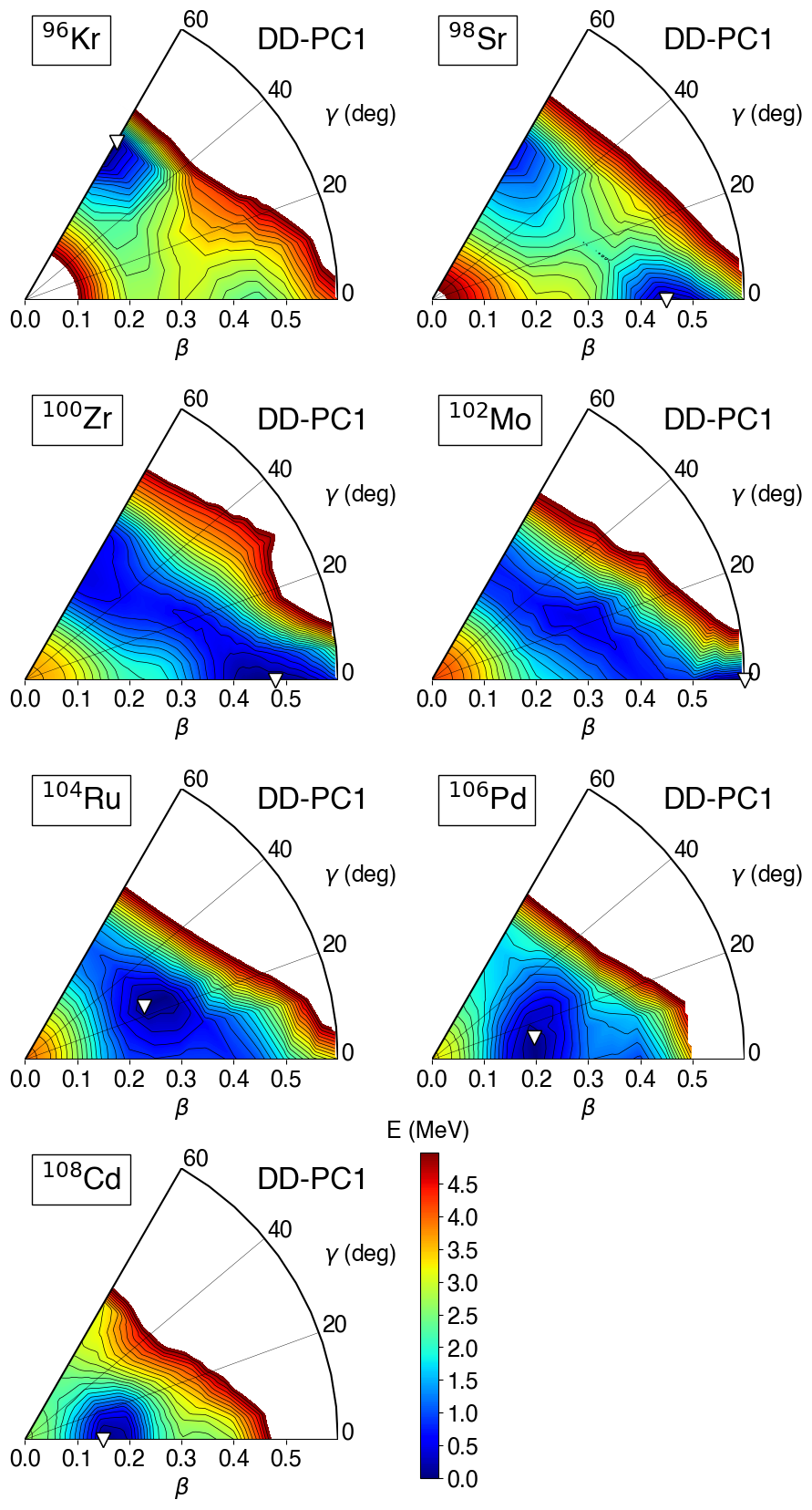
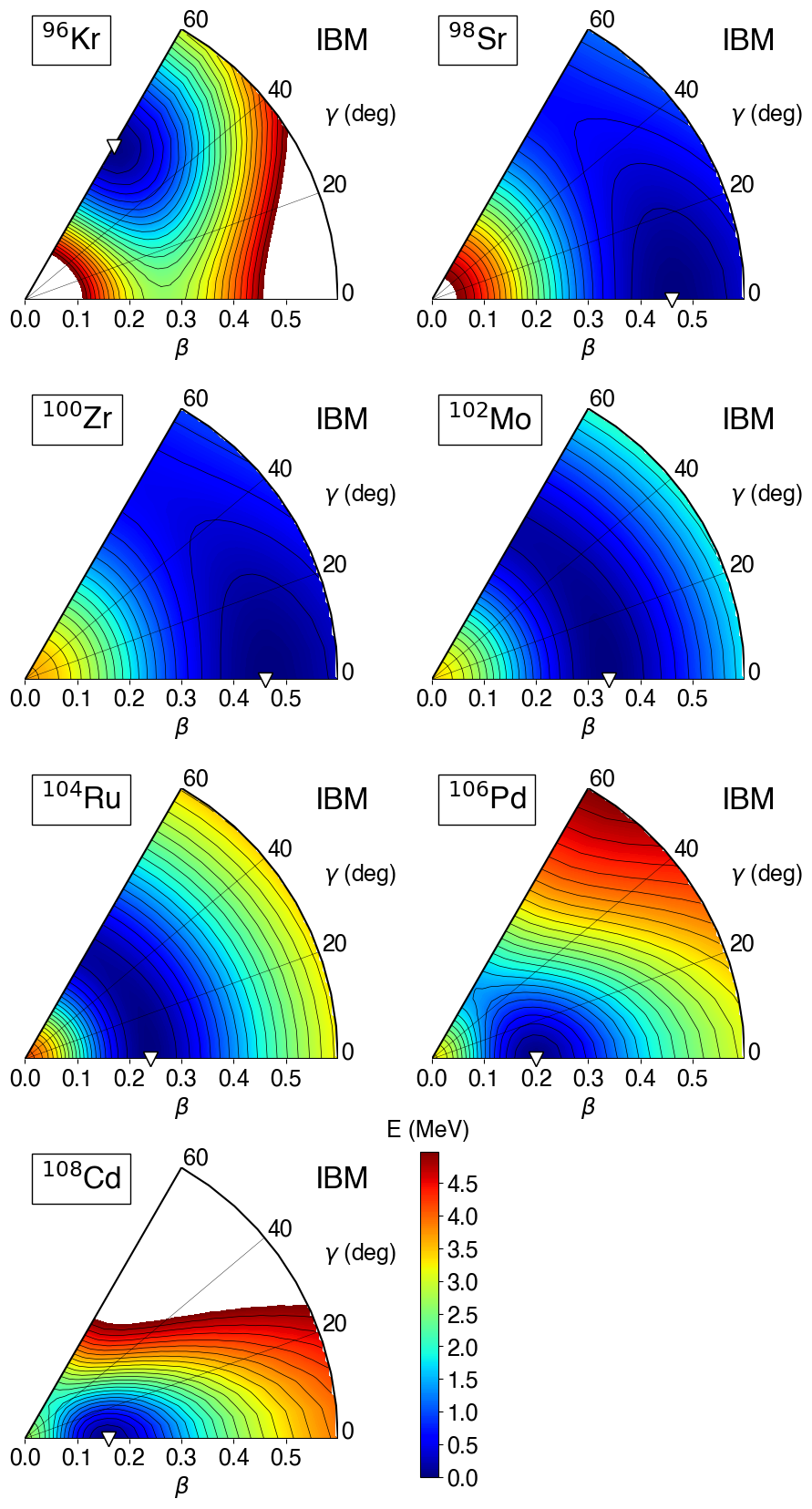
Figure 1: (The first and second columns) Contour plots of the triaxial quadrupole $(\beta,\gamma)$ PESs for the even-even $N=60$ isotones calculated within the constrained relativistic Hartree-Bogoliubov method employing the energy functional DD-PC1 and separable pairing force of finite range. (The third and fourth columns) The corresponding mapped PESs in the IBM-2. The global minimum is indicates by an open triangle, and the difference between the neighboring contours is 0.2 MeV.

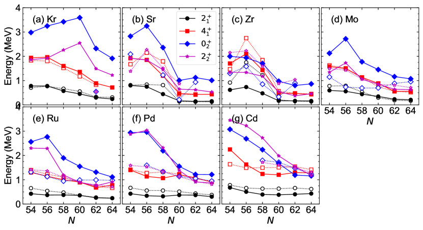
Figure 2: Calculated excitation spectra of the $2^{+}_{1}$, $4^{+}_{1}$, $0^{+}_{2}$, and $2^{+}_{2}$ states of the even-even Kr, Sr, Zr, Mo, Ru, Pd, and Cd isotopes (solid symbols connected by solid lines). The experimental data (open symbols connected by dotted lines) are adopted from NNDC data base [67].

III Low-lying structure of the initial and final nuclei

III.1 Potential energy surfaces

In the first and second columns of Fig. 1 the triaxial quadrupole $(\beta,\gamma)$ PESs for the $N=60$ isotones, from ⁹⁶Kr to ¹⁰⁸Cd, computed within the constrained RHB method with the DD-PC1 EDF and a separable pairing force, are shown. For ⁹⁶Kr and ⁹⁸Sr the SCMF calculation predicts two minima on the oblate and prolate sides of the PESs. The energy surfaces for ¹⁰⁰Zr, ¹⁰²Mo, and ¹⁰⁴Ru are particularly soft in $\gamma$ deformation. For ¹⁰⁴Ru a triaxial minimum around $\gamma\approx 30^{\circ}$ is found. The nuclei ¹⁰⁶Pd and ¹⁰⁸Cd are suggested to be more weakly (prolate) deformed, as they are rather close to the proton $Z=50$ major shell closure.

The SCMF PESs can be compared with the mapped IBM-2 PESs, which are shown in the third and fourth columns of Fig. 1. One could observe certain similarities between the IBM-2 and SCMF PESs, in that basic characteristics of the latter in the neighborhood of the global minimum are reproduced in the former. The difference between the SCMF and IBM-2 PESs becomes more visible for those configurations that correspond to large $\beta$ deformation, so that the IBM-2 surface is flat as compared to the SCMF one. This is due to the restricted degrees of freedom in the IBM-2 framework, that is, the IBM-2 is built only on the valence nucleons in one major oscillator shell while the SCMF model comprises all nucleons.

Another notable difference between the SCMF and IBM-2 PESs is that the former exhibits several minima that are close in energy to each other, most spectacularly in ⁹⁶Kr, ⁹⁸Sr, whereas a single minimum is found in the IBM-2 PES. Within the IBM-2 framework, coexistence of more than one different mean-field minima could be produced by the inclusion of the configuration mixing between several different boson spaces differing in boson number by two [68]. Alternatively, cubic, or three-body, boson terms with negative strength parameter could be introduced in the IBM-2 Hamiltonian [15]. These extensions are, however, not made in the present work, mainly because both the configuration mixing and the inclusion of the cubic terms cannot be handled with the current version of the IBFFM-2 code.

Furthermore, as noted earlier the SCMF PES for ¹⁰⁴Ru exhibits a triaxial minimum at $\gamma\approx 30^{\circ}$, while the IBM-2 one does not. This discrepancy could be solved by including the three-body boson terms with a positive strength parameter [50]. However, the contribution of this term is shown to be rather minor in the energy spectra, except for the $\gamma$ band. Since the most important contribution to determine the energy spectra for the odd-odd nuclei, as well as to the $\beta$ decay, is supposed to come from the low-lying yrast states of the even-even nucleus, it appears to be a reasonable approximation to exclude the three-body boson term for the triaxially deformed nuclei.

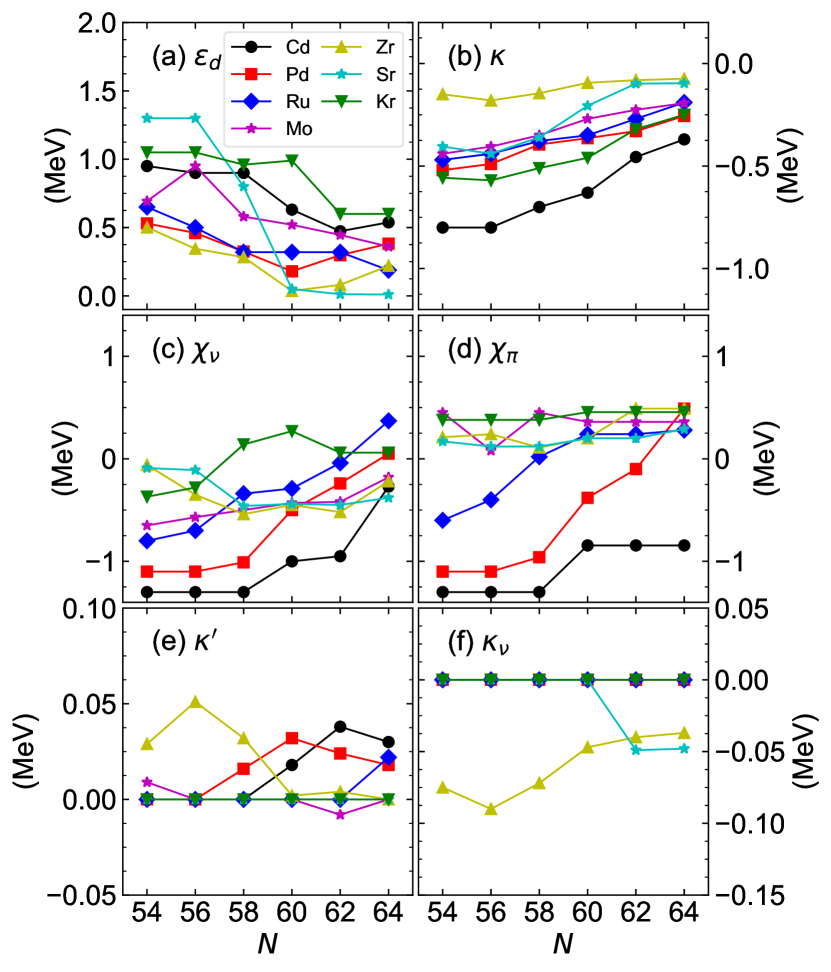
Figure 3: Adopted strength parameters of the IBM-2 Hamiltonian for the even-even nuclei studied in the present work.

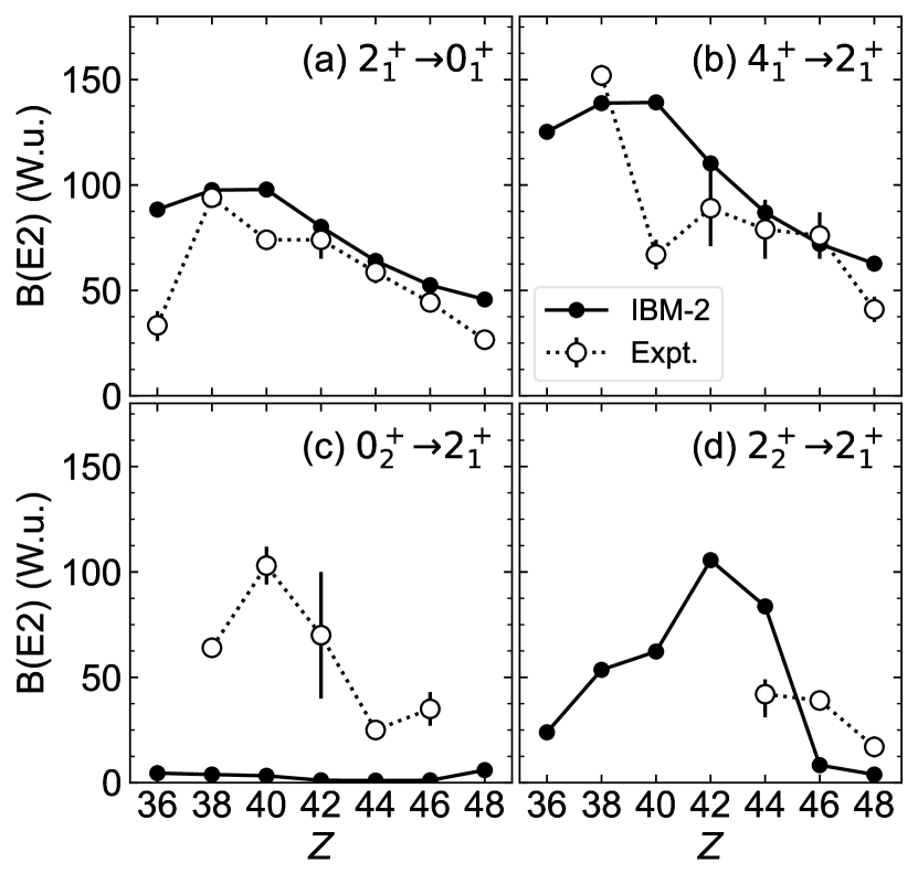
Figure 4: Calculated and experimental [67] (a) $B(E2;2^{+}_{1}\to 0^{+}_{1})$, (b) $B(E2;4^{+}_{1}\to 2^{+}_{1})$, (c) $B(E2;0^{+}_{2}\to 2^{+}_{1})$, and (d) $B(E2;2^{+}_{2}\to 2^{+}_{1})$ transition strengths for the even-even $N=60$ isotones as functions of the proton number $Z$.

III.2 IBM-2 results for the even-even nuclei

Figure 2 depicts the excitation energies of the $2^{+}_{1}$, $4^{+}_{1}$, $0^{+}_{2}$, and $2^{+}_{2}$ states of the even-even Kr, Sr, Zr, Mo, Ru, Pd, and Cd nuclei with $54\leqslant N\leqslant 64$ calculated with the mapped IBM-2. Note that the results for the Zr isotopes have already been presented in Ref. [15], but that are included in the plot for the sake of completeness. One could observe in Fig. 2 that the mapped IBM-2 gives a reasonable description of the observed $2^{+}_{1}$, and $4^{+}_{1}$ excitation energies for all the isotopic chains, except for the Zr one. In may cases, however, the $0^{+}_{2}$ and $2^{+}_{2}$ energy levels are overestimated, in particular, for nearly spherical nuclei close to the $N=50$ magic number, for which the IBM description in general becomes less reliable. For the Sr and Zr isotopes, the calculated low-lying levels exhibit a rapid decrease in energy starting from $N=56$ to 60. This behavior of the levels can be interpreted as a signature of the shape phase transition from the nearly spherical to deformed configurations. The fact that the observed $2^{+}_{1}$ level for ⁹⁶Zr is particularly high reflects the filling of the neutron $d_{5/2}$ subshell closure. As addressed in Ref. [15], the major reason why the mapped IBM-2 is not able to reproduce the level structure of the Zr isotopes in the transitional regions, i.e., $N=56$ and 58, is that the RHB PESs for these nuclei suggest strong deformation and the resultant IBM-2 energy levels are rather compressed. The fact that the calculated $0^{+}_{2}$ levels are systematically higher than the experimental ones is a common occurrence in the mapped IBM-2 calculations. Such a problem could be explained in part by the fact that the underlying EDF calculation generally suggests a too large deformation and one has to choose the quadrupole-quadrupole interaction strength $\kappa$ that is unexpectedly large in magnitude than those which have been often used in phenomenological IBM-2 fitting calculations.

Figure 3 shows evolution of the derived IBM-2 parameters as functions of $N$ employed in the present calculation. One can find some correlations between the aforementioned systematic of the low-lying levels and the IBM-2 parameters. In Fig. 3(a), for instance, the decrease with $N$ of the single $d$ boson energy $\epsilon_{d}$ indicates development of quadrupole deformation. The decrease in magnitude of the parameter $\kappa$ with $N$ also a signature of increasing quadrupole collectivity [Fig. 3(b)]. The average of the parameters, $\chi\equiv(\chi_{\nu}+\chi_{\pi})/2$, and its sign are determined according to whether the nucleus is prolate ($\chi<0$) or oblate ($\chi>0$) deformed in the SCMF calculations. For many of the nuclei, particularly in the Kr, Sr, Zr and Mo isotopes, the average $\chi$ is close to zero, indicating a $\gamma$-softness, as expected from the PESs in Fig. 1. The $\hat{L}\cdot\hat{L}$ term is considered only for those nuclei for which the IB moment of inertia is calculated to be appreciable, i.e., approximately larger than 10. That is the reason why the finite values of the strength parameter $\kappa^{\prime}$ of this term are plotted for a limited number of nuclei in Fig. 3(e).

Figure 4 shows the calculated $B(E2)$ values in Weisskopf units (W.u.) for the even-even $N=60$ isotones. The mapped IBM-2 provides overall a reasonable quantitative and qualitative description of the $B(E2;2^{+}_{1}\to 0^{+}_{1})$ (a) and $B(E2;4^{+}_{1}\to 2^{+}_{1})$ (b) transition strengths, except for the $B(E2;4^{+}_{1}\to 2^{+}_{1})$ value for ¹⁰⁰Zr. As seen from Fig. 4(c) the observed $B(E2;0^{+}_{2}\to 2^{+}_{1})$ rates of the $N=60$ isotones are generally large, that is, of the orders of $>20$ W.u. On the other hand, the mapped IBM-2 suggests too small $B(E2;0^{+}_{2}\to 2^{+}_{1})$ values for all the $N=60$ isotones. The vanishing $B(E2;0^{+}_{2}\to 2^{+}_{1})$ rate implies a too strong deformation. Particularly large $B(E2;0^{+}_{2}\to 2^{+}_{1})$ values of $>60$ W.u. that are found experimentally for the ⁹⁸Sr, ¹⁰⁰Zr, and ¹⁰²Mo are considered to be a consequence of strong shape mixing. This is, however, not accounted for in the mapped IBM-2 framework, since it does not include the effect of configuration mixing. From Fig. 4(d) enhanced $B(E2;2^{+}_{2}\to 2^{+}_{1})$ transition rates are predicted in the IBM-2 calculation. This transition is often considered as an indicator of the $\gamma$ softness, which is indeed shown to be most significant around ¹⁰²Mo and ¹⁰⁴Ru in the corresponding SCMF PESs (see Fig. 1).

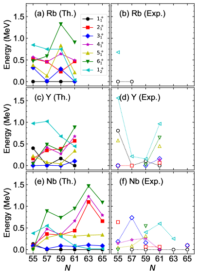
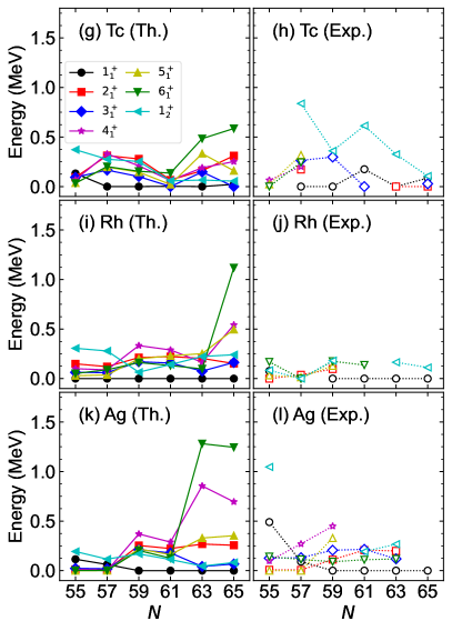
Figure 5: Calculated and experimental excitation energies of the low-spin positive-parity states of the odd-odd nuclei.

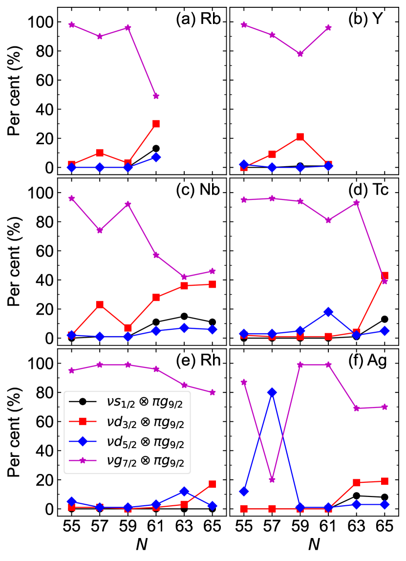
Figure 6: Fractions in percent of the configurations in terms of the pair components $[\nu s_{1/2}\otimes\pi g_{9/2}]^{(J)}$, $[\nu d_{3/2}\otimes\pi g_{9/2}]^{(J)}$, $[\nu d_{5/2}\otimes\pi g_{9/2}]^{(J)}$ and $[\nu g_{7/2}\otimes\pi g_{9/2}]^{(J)}$ that are coupled to even-even boson cores in the IBFFM-2 wave function of the $1^{+}_{1}$ state for the studied odd-odd nuclei.

III.3 IBFFM-2 results for the odd-odd nuclei

The calculated excitation spectra of the low-lying positive-parity states of the considered odd-odd Rb, Y, Nb, Tc, Rh, and Ag nuclei are presented in Fig. 5 in comparison with the available experimental data [67]. For Rb and Y isotopes calculations are made only for those nuclei for which experimental information is available or the same strength parameters of the IBFFM-2 Hamiltonian as those fitted to the available data on neighboring nuclei are used (for Rb). Theoretical results for ¹⁰⁰Rb and ¹⁰²Rb are therefore not shown in the figure. Theoretical energies for ¹⁰²Y and ¹⁰⁴Y are also not shown. This is because of the limitation of the present version of the IBFFM-2 code, which is unable to handle the dimension of the IBFFM-2 Hamiltonian matrices for these nuclei.

One observes, in Fig. 5, characteristic behaviors of the energy levels at particular isotopes within the range $N=57-61$, corresponding to the shape phase transition, and accompanied by the change of the ground-state spin. Rapid evolution of energy levels within that range of the neutron number is most clearly seen, both theoretically and experimentally, in the Y isotopic chain for which even-even Sr nuclei are taken as the boson cores. The rapid structural evolution reflects a phase transitional behavior at $N\approx 60$ of spectroscopic properties of the even-even Sr isotopes [see, Fig. 2(b)]. One can see from Fig. 5 that for the Nb, Tc, Rh, and Ag isotopic chains majority of the isotopes with $N\geqslant 59$ have the $1^{+}$ state as the lowest-energy positive-parity state, while near the neutron shell closure $N=50$ those states with spin higher than $1^{+}$ become the ground state.

Table 2 lists the adopted strength parameters for the IBFFM-2 Hamiltonian, i.e., those for the boson-fermion interactions ($\Gamma_{\nu}$, $\Gamma_{\pi}$, $\Lambda_{\nu}$, $\Lambda_{\pi}$, $A_{\nu}$ and $A_{\pi}$) and for the residual fermion-fermion interactions ($v_{\mathrm{t}}$). In the present calculations, the $\delta$-type and tensor interactions turn out to be most important to reproduce the low-energy spectra of odd-odd nuclei. Fixed values are used for the strength parameter for the $\delta$ term, $v_{\mathrm{d}}=-0.08$ MeV, and that for the spin-spin-$\delta$ term is set to zero, $v_{\mathrm{ssd}}=0$ MeV. The spin-spin term is also assumed to be zero, but is introduced specifically for the ⁹⁸Tc and ⁹⁶Nb nuclei, with the corresponding strengths being $v_{\mathrm{ss}}=0.1$ MeV for both nuclei, in order to reproduce the ground-state spin of $6^{+}$. The energy of the $1^{+}$ states turns out to be quite sensitive to the tensor interaction strength, $v_{\mathrm{t}}$. As seen in Table 2, the adopted $v_{\mathrm{t}}$ strength indeed varies from one nucleus to another in order that the $1^{+}$ state be the ground state in many of the nuclei.

Table 2: Adopted strength parameters (in MeV units) for the boson-fermion interactions, and fermion-fermion interactions in the IBFFM-2 Hamiltonian describing the considered odd-odd nuclei. The fixed values, $v_{\mathrm{d}}=-0.08$ MeV, $v_{\mathrm{ssd}}=0.0$ MeV, are employed for the $\delta$ and spin-spin-$\delta$ terms, respectively. The spin-spin interaction strength, $v_{\mathrm{ss}}$, is chosen to be zero for all nuclei, but for $v_{\mathrm{ss}}=0.1$ MeV for ⁹⁸Tc and ⁹⁶Nb.

Nucleus	$\Gamma_{\nu}$	$\Gamma_{\pi}$	$\Lambda_{\nu}$	$\Lambda_{\pi}$	$A_{\nu}$	$A_{\pi}$	$v_{T}$
102Ag	$0.30$	$0.30$	$0.70$	$1.70$	$-0.50$	$-2.00$	$0.000$
104Ag	$0.30$	$0.30$	$0.70$	$1.70$	$-0.20$	$-0.70$	$0.000$
106Ag	$0.30$	$0.30$	$0.70$	$1.40$	$-0.00$	$-0.70$	$0.060$
108Ag	$0.30$	$0.30$	$0.70$	$1.30$	$-0.00$	$-0.00$	$0.055$
110Ag	$0.10$	$0.30$	$3.00$	$1.30$	$-0.20$	$-0.80$	$0.500$
112Ag	$0.10$	$0.30$	$2.60$	$1.00$	$-0.30$	$-0.00$	$0.700$
100Rh	$0.30$	$0.30$	$0.60$	$1.00$	$-0.00$	$-0.80$	$0.030$
102Rh	$0.30$	$0.30$	$0.20$	$0.35$	$-0.00$	$-0.00$	$0.020$
104Rh	$0.30$	$0.30$	$0.20$	$1.00$	$-0.00$	$-0.80$	$0.055$
106Rh	$0.30$	$0.30$	$0.00$	$1.20$	$-0.00$	$-0.00$	$0.050$
108Rh	$1.50$	$0.30$	$0.70$	$1.00$	$-0.20$	$-0.40$	$0.050$
110Rh	$1.50$	$0.30$	$0.10$	$1.00$	$-0.50$	$-0.50$	$0.400$
98Tc	$0.30$	$0.30$	$0.40$	$0.70$	$-0.00$	$-0.00$	$0.000$
100Tc	$0.30$	$0.30$	$0.35$	$0.90$	$-0.00$	$-0.00$	$0.050$
102Tc	$0.30$	$0.30$	$0.44$	$0.70$	$-0.00$	$-0.00$	$0.040$
104Tc	$0.30$	$0.30$	$0.60$	$2.60$	$-0.40$	$-3.00$	$0.030$
106Tc	$0.30$	$0.30$	$0.30$	$2.10$	$-0.00$	$-3.00$	$0.150$
108Tc	$0.30$	$0.10$	$0.90$	$2.20$	$-1.20$	$-0.00$	$0.500$
96Nb	$0.30$	$0.30$	$0.40$	$0.90$	$-0.00$	$-0.50$	$-0.000$
98Nb	$1.50$	$0.10$	$0.80$	$0.00$	$-1.20$	$-0.00$	$0.280$
100Nb	$1.50$	$0.30$	$0.50$	$0.20$	$-1.40$	$-0.80$	$0.500$
102Nb	$1.50$	$0.10$	$0.90$	$3.80$	$-0.90$	$-2.00$	$0.500$
104Nb	$1.50$	$0.10$	$1.55$	$3.80$	$-0.90$	$-2.00$	$0.800$
106Nb	$1.50$	$0.10$	$1.00$	$3.80$	$-0.30$	$-2.00$	$0.800$
94Y	$0.10$	$1.00$	$0.40$	$0.00$	$-1.00$	$-0.40$	$0.000$
96Y	$0.50$	$1.00$	$0.10$	$0.00$	$-0.00$	$-0.50$	$0.060$
98Y	$0.50$	$1.00$	$0.10$	$0.00$	$-0.00$	$-0.00$	$0.040$
100Y	$0.50$	$0.50$	$0.80$	$12.00$	$-0.80$	$-0.00$	$2.000$
92Rb	$0.30$	$0.50$	$0.40$	$0.00$	$-1.00$	$-0.30$	$0.080$
94Rb	$0.70$	$0.50$	$0.20$	$0.00$	$-2.00$	$-1.00$	$0.100$
96Rb	$0.70$	$0.50$	$0.00$	$0.00$	$-0.00$	$-2.00$	$0.500$
98Rb	$0.30$	$0.10$	$2.20$	$34.00$	$-5.00$	$-5.00$	$0.500$

Table 3: Comparison of the calculated and experimental [67, 69] $B(E2)$ (in W.u.), and $B(M1)$ (in $\mu^{2}_{N}$) transitions, $Q(I)$ (in $e$b), and $\mu(I)$ (in $\mu_{N}$) moments for the odd-odd nuclei considered in this study.

Nucleus	Property	IBFFM-2	Experiment
96Rb	$\mu(2^{+}_{1})$	2.42	$+1.466\pm 0.002$
	$Q(2^{+}_{1})$	$0.48$	$+0.25\pm 0.06$
96Nb	$\mu(6^{+}_{1})$	4.71	$4.976\pm 0.004$
100Nb	$B(M1;1^{+}_{2}\to 1^{+}_{1})$	$0.25$	$0.0038^{+0.0019}_{-0.0010}$
102Ag	$B(E2;6^{+}_{1}\to 5^{+}_{1})$	$0.64$	$32\pm 16$
	$B(M1;6^{+}_{1}\to 5^{+}_{1})$	$1.18$	$0.0011\pm 0.0004$
	$\mu(5^{+}_{1})$	4.38	$+4.6\pm 0.7$
	$\mu(2^{+}_{1})$	5.43	$+4.1\pm 0.3$
	$\mu(7^{+}_{1})$	4.52	$4.6\pm 0.3$
104Ag	$B(M1;6^{+}_{1}\to 5^{+}_{1})$	$0.12$	$>0.0089$
	$B(M1;7^{+}_{1}\to 6^{+}_{1})$	$0.03$	$0.0085\pm 0.0020$
	$B(E2;7^{+}_{1}\to 6^{+}_{1})$	$28.96$	$(1.2\pm 1.1)\times 10^{2}$
	$B(E2;7^{+}_{1}\to 5^{+}_{1})$	$4.37$	$1.4\pm 0.3$
	$\mu(5^{+}_{1})$	3.93	$3.917\pm 0.008$
	$\mu(2^{+}_{1})$	4.88	$+3.7\pm 0.2$
106Ag	$\mu(1^{+}_{1})$	3.03	$+2.9\pm 0.2$
	$Q(6^{+}_{1})$	$0.73$	$+1.08\pm 0.06$
	$\mu(6^{+}_{1})$	4.08	$(+)3.705\pm 0.004$
108Ag	$B(E2;1^{+}_{2}\to 1^{+}_{1})$	$30.61$	$>3.1$
	$B(E2;3^{+}_{1}\to 1^{+}_{1})$	$7.33$	$0.85\pm 0.08$
	$B(M1;2^{+}_{1}\to 1^{+}_{1})$	$0.02$	$>0.012$
	$B(M1;1^{+}_{2}\to 1^{+}_{1})$	$0.00$	$>0.0056$
	$\mu(1^{+}_{1})$	3.00	$2.6884\pm 0.0007$
	$Q(6^{+}_{1})$	$0.89$	$+1.32\pm 0.07$
	$\mu(3^{+}_{1})$	3.33	$3.888\pm 0.015$
	$\mu(6^{+}_{1})$	3.93	$3.58\pm 0.02$
110Ag	$Q(1^{+}_{1})$	$0.06$	$0.24\pm 0.12$
	$\mu(1^{+}_{1})$	3.05	$2.7271\pm 0.0008$
	$Q(6^{+}_{1})$	$-0.03$	$+1.41\pm 0.10$
	$\mu(6^{+}_{1})$	4.19	$+3.607\pm 0.004$
	$\mu(3^{+}_{1})$	3.53	$+3.77\pm 0.03$

Figure 6 exhibits fractions of the pair components denoted $[\nu s_{1/2}\otimes\pi g_{9/2}]^{(J)}$, $[\nu d_{3/2}\otimes\pi g_{9/2}]^{(J)}$, $[\nu d_{5/2}\otimes\pi g_{9/2}]^{(J)}$ and $[\nu g_{7/2}\otimes\pi g_{9/2}]^{(J)}$ in the wave functions of the $1^{+}_{1}$ state of the odd-odd nuclei. In most of the cases shown in the figure the configuration of the $[\nu g_{7/2}\otimes\pi g_{9/2}]^{(J)}$ pairs coupled to the even-even boson cores predominates the $1^{+}_{1}$ wave functions typically for those nuclei with the neutron numbers $N\leqslant 59$. For heavier isotopes with $N$ larger than 59 other pair components start to play a role, especially, the $[\nu d_{3/2}\otimes\pi g_{9/2}]^{(J)}$ ones. The $[\nu s_{1/2}\otimes\pi g_{9/2}]^{(J)}$ pairs do not appear to play an important role.

Table 3 compares the calculated and experimental $B(E2)$ and $B(M1)$ transition rates, and electric quadrupole $Q(I)$ and magnetic dipole $\mu(I)$ moments. One notices that the present IBFFM-2 generally gives a reasonable description of the $Q(I)$ and $\mu(I)$ moments including sign. As for the $B(E2)$ and $B(M1)$ transition rates, however, not much experimental information is available, hence it is rather hard to draw a concrete conclusion about the performance of the IBFFM-2 in computing these observables.

IV $\beta$ decay properties

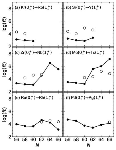
Figure 7: The $\log{ft}$ values for the $\beta^{-}$ decay of the $0^{+}_{1}$ ground-state of even-even nuclei into the $1^{+}_{1}$ state of odd-odd nuclei [panels (a) to (f)], and for the $\beta^{-}$ decay of the $1^{+}_{1}$ state of odd-odd nuclei into the $0^{+}_{1}$ state of even-even nuclei [panels (g) to (l)]. Calculated $\log{ft}$ values are represented by solid circles connected by lines, and open circles denote the experimental values [67].

IV.1 $\log{ft}$ values

GT and Fermi transition strengths are calculated by using the wave functions of the initial and final nuclei provided by the IBM-2, and IBFFM-2 Hamiltonians. The resulting GT and Fermi matrix elements, denoted respectively by $M^{\mathrm{GT}}$ and $M^{\mathrm{F}}$, are used to obtain $ft$ values in second:

$$ft=\frac{6163}{|M^{\mathrm{F}}|^{2}+\left(\frac{g_{\mathrm{A}}}{g_{\mathrm{V}}}\right)^{2}|M^{\mathrm{GT}}|^{2}}\;,$$ (24)

where $g_{\mathrm{A}}=1.27$ and $g_{\mathrm{V}}=1$ are the free values of the axial vector and vector coupling constants, respectively. While some quenching of the $g_{\mathrm{A}}$ factor is often considered in the literature in order to better describe the $\beta$ decay rate, in the following discussion the free $g_{\mathrm{A}}$ value of 1.27 is used.

In Figs. 7(a)–7(f) the calculated $\log{ft}$ values for the $\beta^{-}$ decay of the $0^{+}_{1}$ ground state of even-even nuclei into the $1^{+}_{1}$ state of the odd-odd nuclei are presented as functions of $N$ along each isotopic chain. One notices that these $0^{+}_{1}\to 1^{+}_{1}$ $\beta^{-}$ decay $\log{ft}$ values are systematically lower than the measured ones [67]. This observation applies mainly to those nuclei located before the shape phase transitions, i.e., $N\leqslant 60$, and with lower proton numbers, i.e., Kr, Sr and Zr ones. The fact that the $\log{ft}$ values for the $0^{+}_{1}\to 1^{+}_{1}$ decay are considerably underestimated indicates that enormous amount of quenching would need to be made of the GT transition matrix elements. In the case of the ⁹⁸Sr$(0^{+}_{1})$ $\to$ ⁹⁸Y$(1^{+}_{1})$ decay, for instance, an effective $g_{\mathrm{A}}$ factor that is one order of magnitude smaller than the free value $g_{\mathrm{A}}=1.27$ would be required to reproduce the experimental $\log{ft}$ value of $4.9\pm 0.1$ [67]. The quenching of the GT rates further indicates certain deficiencies of or various assumptions made for the employed nuclear structure models. A possible source of the too small $\log{ft}$ values encountered in the present calculation within the IBFFM-2 is that the single-particle spaces are rather restricted, that is, only the $g_{9/2}$ orbital is considered for the proton single-particle space. This assumption could be reasonable for those isotopes with $Z$ being near the $Z=50$ major shell closure, for which the $g_{9/2}$ orbital plays an predominant role. For the low-$Z$ nuclei rather near the $Z=28$ major shell closure, on the other hand, some other single-particle states such as those coming from outside of the $Z=28-50$ major shell may play a role. There are several other sources of the deficiencies in the description of the $\log{ft}$ values, such as the single (quasi)-particle energies and occupation probabilities used for the boson-fermion interactions in the IBFFM-2 Hamiltonian, the form and parameters of the IBM-2 Hamiltonians for the even-even cores.

The calculated GT matrix element can be analyzed by decomposing it into different components that are associated with different neutron-proton pair configurations. In the same example as above, i.e., ⁹⁸Sr$(0^{+}_{1})$ $\to$ ⁹⁸Y$(1^{+}_{1})$ decay, the dominant contribution to the GT transition arises from the matrix elements of the terms of the forms $[a^{\dagger}_{\nu g_{7/2}}\times a^{\dagger}_{\pi g_{9/2}}]^{(1)}$ and $[\tilde{d}_{\nu}\times[a^{\dagger}_{\nu g_{7/2}}\times a^{\dagger}_{\pi g_{9/2}}]^{(L)}]^{(1)}$ in the corresponding transfer operator. These components are here calculated to be too large in magnitude.

One can also observe in Figs. 7(a)–7(f), that for the $\beta^{-}$ decays of the Zr and Mo isotopes the calculated $\log{ft}$ values exhibit a drastic increase around $N=60$, and are even larger than the measured ones for the heavier Mo nuclei with $N\geqslant 62$. Variation of the $\log{ft}$ values with $N$ looks much more modest for the Ru$(0^{+}_{1})\to$Rh$(1^{+}_{1})$ and Pd$(0^{+}_{1})\to$Ag$(1^{+}_{1})$ $\beta^{-}$ decays. The rapid increase of the $\log{ft}$ values at $N\approx 60$ seems to be correlated with the fact that the neutron-proton pair configuration of the type $[\nu g_{7/2}\otimes\pi g_{9/2}]^{(J)}$ dominates the wave functions of the $1^{+}_{1}$ state of the odd-odd nuclei with $N\leqslant 60$, but that other configurations start to make appreciable contributions for $N>60$ (see, Fig. 6). The different pair components are more or less fragmented in the GT matrix elements for the $N>60$ nuclei, and cancel each other to give rise to the small $M^{\mathrm{GT}}$ or large $\log{ft}$ value.

In a similar fashion, in Figs. 7(g)–7(l) the predicted $\log{ft}$ values for the $\beta^{-}$ decay of the odd-odd nuclei are compared with the experimental data [67]. Data are not available for the Rb$(1^{+}_{1})\to$Sr$(0^{+}_{1})$ decay, and only the lower bound, $\log{ft}>6.9$, of the unidentified $(1)^{-}$ state is known for the ¹⁰⁰Y$(1^{+}_{1})\to^{100}$Zr$(0^{+}_{1})$ decay. A general remark is that in each isotopic chain the calculated $1^{+}_{1}\to 0^{+}_{1}$ $\log{ft}$ value increases as a function of $N$, consistently with the observed systematic, and further exhibits a rapid increase from $N=59$ to 61. The change is particularly significant for the Nb$(1^{+}_{1})\to$Mo$(0^{+}_{1})$ and Tc$(1^{+}_{1})\to$Ru$(0^{+}_{1})$ decays, while for the Rh$(1^{+}_{1})\to$Pd$(0^{+}_{1})$ and Ag$(1^{+}_{1})\to$Cd$(0^{+}_{1})$ ones the predicted $\log{ft}$ values increase more slowly with $N$. In addition, the present calculation reproduces the measured $\log{ft}$ values to a greater extent than in the case of the $\beta^{-}$ decay of the even-even nuclei.

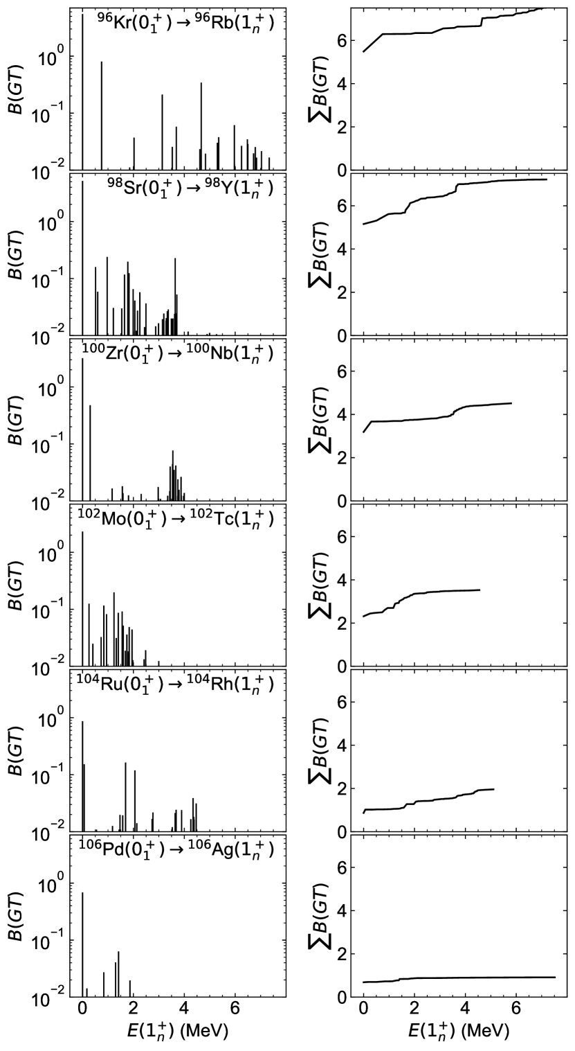
Figure 8: (Left) $B({\mathrm{GT}})$ strength distribution for the $\beta^{-}$ decay $0^{+}_{1}\to 1^{+}_{n}$ of the even-even $N=60$ isotones in terms of the excitation energies of the $1^{+}_{n}$ states of the odd-odd final nuclei, and (right) their running sum.

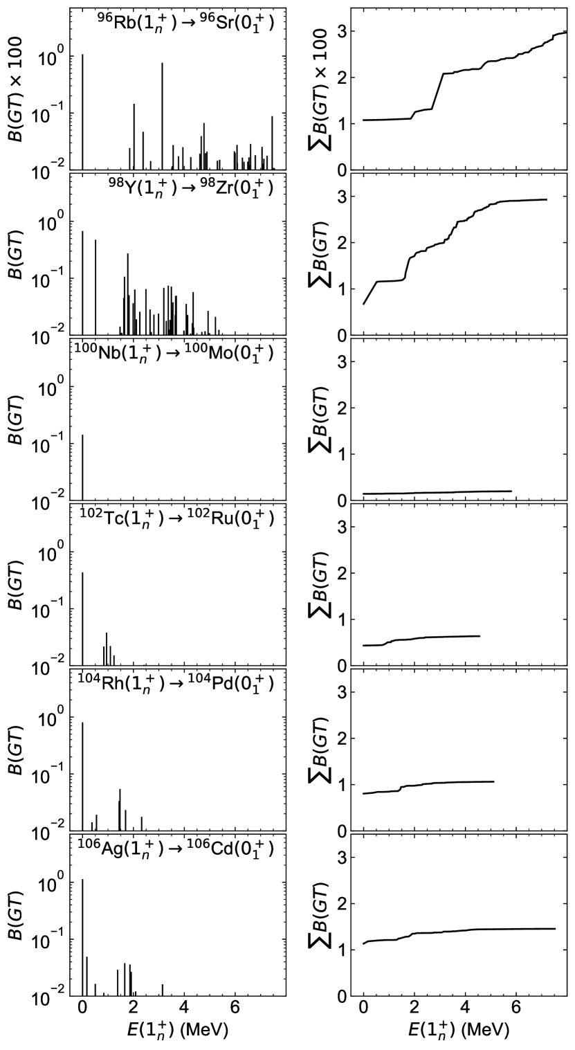
Figure 9: $B({\mathrm{GT}})$ strength distribution for the $\beta^{-}$ decay $1^{+}_{n}\to 0^{+}_{1}$ of the odd-odd $N=59$ isotones in terms of the excitation energies of the $1^{+}_{n}$ states of the odd-odd initial nuclei, and (right) their running sum. Note that the $B({\mathrm{GT}})$ and the sums $\sum B({\mathrm{GT}})$ for the ⁹⁶Rb$(1^{+}_{n})\to^{96}$Sr$(0^{+}_{1})$ are too small, and that are scaled with a factor 100 so that they are more visible.

IV.2 GT strength distributions

On the left-hand side of Fig. 8 distributions of the $B(GT)$ transition strengths, $B({\textnormal{GT}};0^{+}_{1}\to 1^{+}_{1})=|M^{\mathrm{GT}}(0^{+}_{1}\to 1^{+}_{1})|^{2}$, for the $\beta^{-}$ decay of the even-even $N=60$ isotones are shown as functions of the $1^{+}$ excitation energies $E(1^{+}_{n})$ below 8 MeV. For each odd-odd nucleus, all the $1^{+}$ states resulting from the IBFFM-2 and the corresponding GT transitions are here considered. For most of the even-even nuclei shown in the figure, the GT transition to the first excited $1^{+}_{1}$ is the strongest, while contributions from the decays to higher lying $1^{+}$ states become more minor with the increasing $1^{+}$ excitation energy. For the ¹⁰⁴Ru$(0^{+}_{1})\to^{104}$Rh$(1^{+})$ decay, in particular, non-negligible amounts of the GT transitions are predicted within the excitation energies $E(1^{+}_{n})$ from around 2 MeV to 4 MeV. A similar degree of the fragmentation of the $B({\mathrm{GT}})$ strength distributions are obtained for the ¹⁰²Mo$\to^{102}$Tc decay below $E(1^{+}_{n})\approx 2$ MeV.

In addition, running sums of the GT strengths, i.e., $\sum_{n}B({\textnormal{GT}};0^{+}_{1}\to 1^{+}_{n})$, that are taken up to the excitation energy of the highest lying $1^{+}$ state are shown on the right-hand side of Fig. 8. For most of the considered $\beta^{-}$ decays, the sums appear to converge at low excitation energy, typically of $E(1^{+})\leqslant 4$ MeV. Notably for the ⁹⁶Kr$(0^{+}_{1})\to^{96}$Rb$(1^{+})$ and ¹⁰⁴Ru$(0^{+}_{1})\to^{104}$Rh$(1^{+})$ decays, the sums continue to increase up to the excitation energies of the highest-lying $1^{+}$ states obtained with the IBFFM-2. The GT decay rates are predicted to be remarkably large for the low-$Z$ isotones, i.e., ⁹⁶Kr and ⁹⁸Sr, with the corresponding running sums reaching $\sum_{n}B(\textnormal{GT};0^{+}_{1}\to 1^{+}_{n})\approx 7.5$, but that becomes smaller for the higher-$Z$ isotones, e.g., ¹⁰⁶Pd, with the final sum $\sum_{n}B(\textnormal{GT};0^{+}_{1}\to 1^{+}_{n})<1$. This conforms to the results shown in Fig. 7 that the calculated $\log{ft}$ values for the GT transition of the even-even nuclei to the lowest $1^{+}$ state of the odd-odd nuclei are particularly small for the low-$Z$ nuclei such as Kr and Sr ones.

Figure 9 depicts, on the left-hand side, the $B({\mathrm{GT}})$ strength distributions, $B({\textnormal{GT}}:1^{+}_{1}\to 0^{+}_{1})=|M^{\mathrm{GT}}(1^{+}_{1}\to 0^{+}_{1})|^{2}/3$, for the $\beta^{-}$ decays of the odd-odd $N=59$ isotones into the even-even $N=58$ isotones in terms of the $E(1^{+})$ excitation energy. In general, the GT strengths for the odd-odd isotones are predicted to be smaller, $<1.0$, than those for the even-even nuclei, which are larger than 1 (see Fig. 8). As in the case of the $\beta^{-}$ decays of the even-even nuclei, shown in Fig. 8, contributions from the low-lying $1^{+}$ are dominant for the $\beta^{-}$ decays of ¹⁰⁰Nb, ¹⁰²Tc, ¹⁰⁴Rh, and ¹⁰⁶Ag. Of particular interest are the ⁹⁶Rb$(1^{+})\to^{96}$Sr$(0^{+}_{1})$ and ⁹⁸Y$(1^{+})\to^{98}$Zr$(0^{+}_{1})$ decays. For these decay processes, $B({\mathrm{GT}})$ strength distribution exhibits a substantial degree of fragmentation, and contributions from the nonyrast $1^{+}$ states are as significant as that from the lowest $1^{+}$ state. Note that, as for the $B({\mathrm{GT}})$ rate of the ⁹⁶Rb$(1^{+})\to^{96}$Sr$(0^{+}_{1})$ decay, the $B({\mathrm{GT}})$ rates are negligibly small, so that they are scaled with a factor 100 in the figure. On the right-hand side of the same figure shown are the running sums $\sum B(\textnormal{GT};1^{+}_{n}\to 0^{+}_{1})$. The sum steadily increases as a function of the $E(1^{+})$ excitation energy for the ⁹⁶Rb and ⁹⁸Y decays, since the contributions from higher-lying $1^{+}$ states are non-negligible. The final sum at the $E(1^{+})$ energy corresponding to the highest $1^{+}$ state becomes larger for the decay of the odd-odd nuclei as a function of the proton number $Z$, that is, the sum reaches $\sum_{n}B({\mathrm{GT}})\approx 0.03$, 2.9, 0.2, 0.64, 1.1 and 1.5 for the decays of ⁹⁶Rb, ⁹⁸Y, ¹⁰⁰Nb, ¹⁰²Tc, ¹⁰⁴Rh, and ¹⁰⁶Ag, respectively. For the ⁹⁸Y$(1^{+})\to^{98}$Zr$(0^{+}_{1})$ decay, however, the running sum ends up with a particularly large value, $\sum_{n}B({\mathrm{GT}})\approx 2.9$, reflecting that the GT strengths are calculated to be exceptionally large. The too large $B({\mathrm{GT}})$ values are due to the fragmentation of the different pair components in the GT transition matrix, many of which are suppose to cancel each other.

To summarize the results shown in Figs. 8 and 9, it appears that the GT transitions of the lowest or low-lying $1^{+}$ states make dominant roles in the running sums of the $B({\mathrm{GT}})$ strengths for the $\beta^{-}$ decays of both the even-even and odd-odd nuclei, while the fragmentation tends to occur for those nuclei far from the proton $Z=50$ major shell closure. This observation seems compatible, to a good extent, to the single-state dominance [70, 71] or the low-lying state dominance [72] proposed especially for the studies of double-$\beta$ decay. The previous mapped IBM-2 calculation in Ref. [55] has also provided a similar conclusion on the $2\nu\beta\beta$ decay NMEs of a number of candidate nuclei.

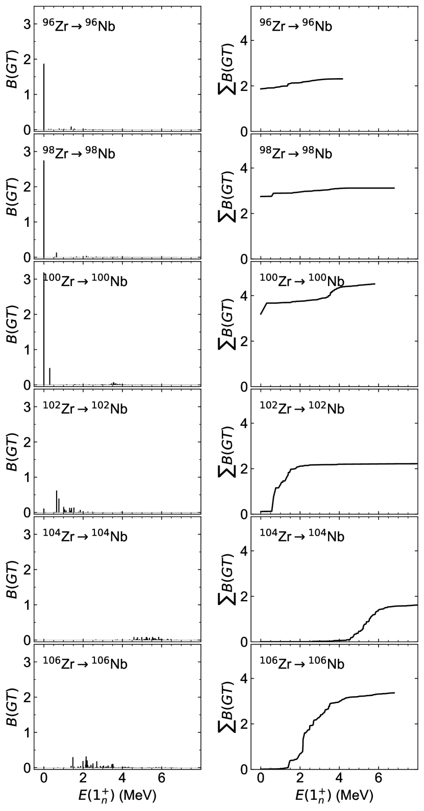
Figure 10: Same as Fig. 8, but for the Zr isotopes.

It should be also worth investigating how the GT strength distribution changes along a given isotopic chain. For that purpose, the $B({\mathrm{GT}})$ strength distributions and their running sums for $\beta^{-}$ decays of the even-even Zr isotopes are shown in Fig. 10. For ⁹⁶Zr, ⁹⁸Zr, and ¹⁰⁰Zr, the GT strength is almost solely accounted for by the transition to the first $1^{+}$ state, which is also considerably large in magnitude, $B(\textnormal{GT};0^{+}_{1}\to 1^{+}_{1})\approx 2-3$. On the other hand, one notices for the heavier Zr nuclei, i.e., ¹⁰²Zr, ¹⁰⁴Zr, and ¹⁰⁶Zr, that the GT strength is fragmented to a great extent. Particularly for the ¹⁰⁴Zr$(0^{+}_{1})\to^{104}$Nb$(1^{+})$ decay, major contribution to the total GT strength comes from the transitions to the $1^{+}$ states that are at the excitation energy $E(1^{+})$ of about 4-6 MeV, while the $B(\textnormal{GT};0^{+}_{1}\to 1^{+}_{1})$ transitions does not play a significant role. For the lighter Zr nuclei, e.g., ⁹⁶Zr and ⁹⁸Zr, the sum, $\sum_{n}B({\mathrm{GT}})$, appears to be converged at relatively low $E(1^{+})$ excitation energies, $E(1^{+})\approx$ 2 MeV, whereas for the heavier ones the convergence seems to occur at higher $E(1^{+})$ excitation energies, e.g., $E(1^{+})>4$ MeV for ¹⁰⁴Zr and ¹⁰⁶Zr.

Table 4: Comparison of calculated and observed [67] $\log{ft}$ values for the $\beta^{-}$ decay of the even-mass nuclei including the $N=60$ isotones.

		$\log{ft}$
Decay	$I\to I^{\prime}$	Th.	Exp.
98Rb$\to^{98}$Sr	$3^{+}_{1}\to 2^{+}_{1}$	7.78	5.6
	$3^{+}_{1}\to 2^{+}_{2}$	9.95	6.2
	$3^{+}_{1}\to 2^{+}_{3}$	8.44	6.1
	$3^{+}_{1}\to 4^{+}_{1}$	7.90	6.3
98Sr$\to^{98}$Y	$0^{+}_{1}\to 1^{+}_{1}$	2.87	$4.9\pm 0.1$
	$0^{+}_{1}\to 1^{+}_{2}$	4.38	$4.4\pm 0.1$
	$0^{+}_{1}\to 1^{+}_{3}$	4.82	$5.5\pm 0.1$
	$0^{+}_{1}\to 1^{+}_{4}$	4.20	$5.6\pm 0.1$
100Y$\to^{100}$Zr	$4^{+}_{1}\to 4^{+}_{1}$	5.46	$\approx 6.0$
	$4^{+}_{1}\to 3^{+}_{1}$	4.22	$>6.5$
	$4^{+}_{1}\to 4^{+}_{2}$	4.54	$>6.6$
	$4^{+}_{1}\to 4^{+}_{3}$	4.83	$>6.9$
100Zr$\to^{100}$Nb	$0^{+}_{1}\to 1^{+}_{1}$	3.08	$4.6\pm 0.1$
	$0^{+}_{1}\to 1^{+}_{2}$	3.90	$4.8\pm 0.1$
	$0^{+}_{1}\to 1^{+}_{3}$	6.50	$5.8$
	$0^{+}_{1}\to 1^{+}_{4}$	6.34	$4.5\pm 0.1$
102Nb$\to^{102}$Mo	$4^{+}_{1}\to 4^{+}_{1}$	7.51	$6.44$
	$4^{+}_{1}\to 3^{+}_{1}$	6.45	$6.21$
	$4^{+}_{1}\to 4^{+}_{2}$	7.45	$6.31$
	$4^{+}_{1}\to 3^{+}_{2}$	6.20	$4.86$
	$1^{+}_{1}\to 0^{+}_{1}$	5.82
	$1^{+}_{1}\to 0^{+}_{2}$	6.99
	$1^{+}_{1}\to 2^{+}_{1}$	6.72
	$1^{+}_{1}\to 2^{+}_{2}$	7.53
102Mo$\to^{102}$Tc	$0^{+}_{1}\to 1^{+}_{1}$	3.22	$4.21\pm 0.09$
	$0^{+}_{1}\to 1^{+}_{2}$	4.48	$5.74\pm 0.10$
	$0^{+}_{1}\to 1^{+}_{3}$	5.19	$4.81\pm 0.09$
104Tc$\to^{104}$Ru	$3^{+}_{1}\to 2^{+}_{1}$	6.22	$8.10\pm 0.07$
	$3^{+}_{1}\to 4^{+}_{1}$	6.91	$8.34\pm 0.09$
	$3^{+}_{1}\to 2^{+}_{2}$	5.63	$8.14\pm 0.09$
	$3^{+}_{1}\to 3^{+}_{1}$	7.83	$8.18\pm 0.10$
106Rh$\to^{106}$Pd	$1^{+}_{1}\to 0^{+}_{1}$	4.46	$5.168\pm 0.007$
	$1^{+}_{1}\to 2^{+}_{1}$	4.11	$5.865\pm 0.017$
	$1^{+}_{1}\to 2^{+}_{2}$	7.72	$6.55\pm 0.07$
	$1^{+}_{1}\to 0^{+}_{2}$	6.45	$5.354\pm 0.019$
	$1^{+}_{1}\to 2^{+}_{3}$	6.48	$5.757\pm 0.017$
	$1^{+}_{1}\to 2^{+}_{4}$	6.35	$6.25\pm 0.03$
	$1^{+}_{1}\to 2^{+}_{5}$	5.06	$5.83\pm 0.03$
	$1^{+}_{1}\to 0^{+}_{3}$	7.15	$5.51\pm 0.05$
	$1^{+}_{1}\to 2^{+}_{6}$	7.52	$6.59\pm 0.10$
	$1^{+}_{1}\to 0^{+}_{4}$	7.62	$5.63\pm 0.07$
108Ag$\to^{108}$Cd	$1^{+}_{1}\to 0^{+}_{1}$	3.74	$4.425\pm 0.009$
	$1^{+}_{1}\to 2^{+}_{1}$	6.06	$5.35\pm 0.03$

Table 5: Same as Table 4, but for the EC decay.

		$\log{ft}$
Decay	$I\to I^{\prime}$	Th.	Exp.
104Rh$\to^{104}$Ru	$1^{+}_{1}\to 0^{+}_{1}$	4.12	$4.32\pm 0.11$
	$1^{+}_{1}\to 2^{+}_{1}$	6.26	$5.42\pm 0.06$
	$1^{+}_{1}\to 0^{+}_{2}$	4.93	$5.15\pm 0.18$
106Ag$\to^{106}$Pd	$1^{+}_{1}\to 0^{+}_{1}$	4.22	$4.92$
	$1^{+}_{1}\to 2^{+}_{1}$	5.02	$5.24$
	$1^{+}_{1}\to 0^{+}_{2}$	4.48	$6.5$
	$1^{+}_{1}\to 2^{+}_{2}$	5.74	$6.5$
	$1^{+}_{1}\to 0^{+}_{3}$	5.32	$7.0$
	$1^{+}_{1}\to 2^{+}_{3}$	5.02	$7.9$
	$1^{+}_{1}\to 0^{+}_{4}$	5.88	$6.1$
	$1^{+}_{1}\to 2^{+}_{4}$	5.93	$6.9$
	$1^{+}_{1}\to 0^{+}_{5}$	6.65	$7.6$
	$1^{+}_{1}\to 2^{+}_{5}$	4.40	$6.8$
	$6^{+}_{1}\to 6^{+}_{1}$	8.95	$8.02\pm 0.24$
	$6^{+}_{1}\to 5^{+}_{1}$	7.74	$5.087\pm 0.018$
	$6^{+}_{1}\to 5^{+}_{2}$	7.57	$5.08\pm 0.5$

Besides the transitions between the $0^{+}_{1}$ and $1^{+}_{1}$ states, there are experimental data for the $\log{ft}$ values for the decays between states with spin other than $1^{+}$ and between higher-lying $0^{+}$ and $1^{+}$ states. To keep the discussion as simple as possible, let us focus on the $\beta$ decays that only involve the even-even $N=60$ isotones. The calculated and experimental [67] $\log{ft}$ values of the $\beta^{-}$ and electron-capture (EC) decays are listed in Table 4 and Table 5 list, respectively. As one can see from Table 4, it is rather hard to draw a solid conclusion on the quality of the mapped IBM-2 framework for the description of the $\log{ft}$ values for many different $\beta^{-}$ decays. Nevertheless, for many of low-$Z$ nuclei the present calculation gives smaller $\log{ft}$ values than the experimental ones, suggesting that the assumption of considering only the single proton orbital ($\pi g_{9/2}$) may not be reasonable, and that the $\log{ft}$ calculations are also influenced by the chosen parameters or forms of the IBFFM-2 Hamiltonian. The calculation, on the other hand, overestimates the measured $\log{ft}$ values for higher-$Z$ nuclei. Experimental data for the $\log{ft}$ values for the EC decay are available for the ¹⁰⁴Rh and ¹⁰⁶Ag nuclei. Overall, the present calculation reproduces the available $\log{ft}$ data fairly well especially for those nuclei that are not very far from the proton $Z=50$ major shell.

V Summary and conclusions

The low-energy structure and $\beta$-decay properties of the neutron-rich even-mass nuclei around $N=60$ that are currently of much interest experimentally have been studied within the theoretical framework of the EDF-to-IBM mapping. The IBM-2 Hamiltonian for the even-even core nuclei, and particle-boson interactions have been determined by using the results of the triaxial quadrupole constrained SCMF calculations within the RHB model with the DD-PC1 functional and the separable pairing force. By using the wave functions for the initial and final nuclei obtained from the IBM-2 and IBFFM-2, the GT and Fermi transition strengths have been computed, for which no adjustable parameter is introduced.

The calculated $(\beta,\gamma)$ potential energy surfaces for the $N=60$ even-even isotones suggest for most cases notably $\gamma$-soft shapes that vary substantially with $Z$. Spectroscopic calculations for the even-even Kr, Sr, Zr, Mo, Ru, Pd, and Cd isotopes using the mapped IBM-2 have shown evolution of the low-lying energy spectra and $B(E2)$ rates as functions of $N$, and rapid changes of these observables around $N=60$ for the Sr, Zr, and Mo chains. The excitation spectra of low-spin states of the neighboring odd-odd nuclei have been shown to exhibit certain variation with $N$, reflecting the shape transitions that occur in the even-even core nuclei.

The mapped IBM-2 has provided the $\log{ft}$ values for the $\beta^{-}$ decays of the $0^{+}_{1}$ state of the even-even nuclei into the $1^{+}_{1}$ state of the odd-odd nuclei that are systematically lower than the experimental values for the lower-$Z$ isotopes (i.e., Kr, Sr and Zr) and mostly for $N\leqslant 60$. The too small $\log{ft}$ values, that is, too large GT transition rates, in the above nuclear systems indicate a need for substantial quenching of the $g_{\mathrm{A}}$ factor, which amounts to an order of magnitude in some cases. The necessity of introducing effective $g_{\mathrm{A}}$ factors would then imply deficiencies of the theoretical framework that arise from various model assumptions and approximations, including the particular choice of the EDF providing microscopic input to the IBM-2 and IBFFM-2, the form of the corresponding Hamiltonians, and the restricted single-particle space.

The simultaneous calculation of the low-energy nuclear structure and $\beta$ decay will be useful for improving the quality of the employed theoretical method in describing spectroscopic properties of individual nuclei even more accurately, and will provide implications for studies of other fundamental nuclear processes including the double-$\beta$ decay in the region of interest.

References

- Cejnar et al. [2010] P. Cejnar, J. Jolie, and R. F. Casten, Rev. Mod. Phys. 82, 2155 (2010).
- Heyde and Wood [2011] K. Heyde and J. L. Wood, Rev. Mod. Phys. 83, 1467 (2011).
- Caurier et al. [2005] E. Caurier, G. Martínez-Pinedo, F. Nowacki, A. Poves, and A. P. Zuker, Rev. Mod. Phys. 77, 427 (2005).
- Sieja et al. [2009] K. Sieja, F. Nowacki, K. Langanke, and G. Martínez-Pinedo, Phys. Rev. C 79, 064310 (2009).
- Togashi et al. [2016] T. Togashi, Y. Tsunoda, T. Otsuka, and N. Shimizu, Phys. Rev. Lett. 117, 172502 (2016).
- Shimizu et al. [2017] N. Shimizu, T. Abe, M. Honma, T. Otsuka, T. Togashi, Y. Tsunoda, Y. Utsuno, and T. Yoshida, Physica Scripta 92, 063001 (2017).
- Bender et al. [2003] M. Bender, P.-H. Heenen, and P.-G. Reinhard, Rev. Mod. Phys. 75, 121 (2003).
- Vretenar et al. [2005] D. Vretenar, A. V. Afanasjev, G. A. Lalazissis, and P. Ring, Phys. Rep. 409, 101 (2005).
- Nikšić et al. [2011] T. Nikšić, D. Vretenar, and P. Ring, Prog. Part. Nucl. Phys. 66, 519 (2011).
- Mei et al. [2012] H. Mei, J. Xiang, J. M. Yao, Z. P. Li, and J. Meng, Phys. Rev. C 85, 034321 (2012).
- Robledo et al. [2019] L. M. Robledo, T. R. Rodríguez, and R. R. Rodríguez-Guzmán, J. Phys. G: Nucl. Part. Phys. 46, 013001 (2019).
- Iachello and Arima [1987] F. Iachello and A. Arima, The interacting boson model (Cambridge University Press, Cambridge, 1987).
- Nomura et al. [2016a] K. Nomura, R. Rodríguez-Guzmán, and L. M. Robledo, Phys. Rev. C 94, 044314 (2016a).
- García-Ramos and Heyde [2020] J. E. García-Ramos and K. Heyde, Phys. Rev. C 102, 054333 (2020).
- Nomura et al. [2020a] K. Nomura, T. Nikšić, and D. Vretenar, Phys. Rev. C 102, 034315 (2020a).
- Gavrielov et al. [2022] N. Gavrielov, A. Leviatan, and F. Iachello, Phys. Rev. C 105, 014305 (2022).
- Dillmann et al. [2003] I. Dillmann, K.-L. Kratz, A. Wöhr, O. Arndt, B. A. Brown, P. Hoff, M. Hjorth-Jensen, U. Köster, A. N. Ostrowski, B. Pfeiffer, D. Seweryniak, J. Shergur, and W. B. Walters (the ISOLDE Collaboration), Phys. Rev. Lett. 91, 162503 (2003).
- Nishimura et al. [2011] S. Nishimura, Z. Li, H. Watanabe, K. Yoshinaga, T. Sumikama, T. Tachibana, K. Yamaguchi, M. Kurata-Nishimura, G. Lorusso, Y. Miyashita, A. Odahara, H. Baba, J. S. Berryman, N. Blasi, A. Bracco, F. Camera, J. Chiba, P. Doornenbal, S. Go, T. Hashimoto, S. Hayakawa, C. Hinke, E. Ideguchi, T. Isobe, Y. Ito, D. G. Jenkins, Y. Kawada, N. Kobayashi, Y. Kondo, R. Krücken, S. Kubono, T. Nakano, H. J. Ong, S. Ota, Z. Podolyák, H. Sakurai, H. Scheit, K. Steiger, D. Steppenbeck, K. Sugimoto, S. Takano, A. Takashima, K. Tajiri, T. Teranishi, Y. Wakabayashi, P. M. Walker, O. Wieland, and H. Yamaguchi, Phys. Rev. Lett. 106, 052502 (2011).
- Quinn et al. [2012] M. Quinn, A. Aprahamian, J. Pereira, R. Surman, O. Arndt, T. Baumann, A. Becerril, T. Elliot, A. Estrade, D. Galaviz, T. Ginter, M. Hausmann, S. Hennrich, R. Kessler, K.-L. Kratz, G. Lorusso, P. F. Mantica, M. Matos, F. Montes, B. Pfeiffer, M. Portillo, H. Schatz, F. Schertz, L. Schnorrenberger, E. Smith, A. Stolz, W. B. Walters, and A. Wöhr, Phys. Rev. C 85, 035807 (2012).
- Lorusso et al. [2015] G. Lorusso, S. Nishimura, Z. Y. Xu, A. Jungclaus, Y. Shimizu, G. S. Simpson, P.-A. Söderström, H. Watanabe, F. Browne, P. Doornenbal, G. Gey, H. S. Jung, B. Meyer, T. Sumikama, J. Taprogge, Z. Vajta, J. Wu, H. Baba, G. Benzoni, K. Y. Chae, F. C. L. Crespi, N. Fukuda, R. Gernhäuser, N. Inabe, T. Isobe, T. Kajino, D. Kameda, G. D. Kim, Y.-K. Kim, I. Kojouharov, F. G. Kondev, T. Kubo, N. Kurz, Y. K. Kwon, G. J. Lane, Z. Li, A. Montaner-Pizá, K. Moschner, F. Naqvi, M. Niikura, H. Nishibata, A. Odahara, R. Orlandi, Z. Patel, Z. Podolyák, H. Sakurai, H. Schaffner, P. Schury, S. Shibagaki, K. Steiger, H. Suzuki, H. Takeda, A. Wendt, A. Yagi, and K. Yoshinaga, Phys. Rev. Lett. 114, 192501 (2015).
- Caballero-Folch et al. [2016] R. Caballero-Folch, C. Domingo-Pardo, J. Agramunt, A. Algora, F. Ameil, A. Arcones, Y. Ayyad, J. Benlliure, I. N. Borzov, M. Bowry, F. Calviño, D. Cano-Ott, G. Cortés, T. Davinson, I. Dillmann, A. Estrade, A. Evdokimov, T. Faestermann, F. Farinon, D. Galaviz, A. R. García, H. Geissel, W. Gelletly, R. Gernhäuser, M. B. Gómez-Hornillos, C. Guerrero, M. Heil, C. Hinke, R. Knöbel, I. Kojouharov, J. Kurcewicz, N. Kurz, Y. A. Litvinov, L. Maier, J. Marganiec, T. Marketin, M. Marta, T. Martínez, G. Martínez-Pinedo, F. Montes, I. Mukha, D. R. Napoli, C. Nociforo, C. Paradela, S. Pietri, Z. Podolyák, A. Prochazka, S. Rice, A. Riego, B. Rubio, H. Schaffner, C. Scheidenberger, K. Smith, E. Sokol, K. Steiger, B. Sun, J. L. Taín, M. Takechi, D. Testov, H. Weick, E. Wilson, J. S. Winfield, R. Wood, P. Woods, and A. Yeremin, Phys. Rev. Lett. 117, 012501 (2016).
- Navrátil and Dobe [1988] P. Navrátil and J. Dobe, Phys. Rev. C 37, 2126 (1988).
- Dellagiacoma and Iachello [1989] F. Dellagiacoma and F. Iachello, Phys. Lett. B 218, 399 (1989).
- Brant et al. [2004] S. Brant, N. Yoshida, and L. Zuffi, Phys. Rev. C 70, 054301 (2004).
- Yoshida and Iachello [2013] N. Yoshida and F. Iachello, Prog. Theor. Exp. Phys. 2013, 043D01 (2013).
- Mardones et al. [2016] E. Mardones, J. Barea, C. E. Alonso, and J. M. Arias, Phys. Rev. C 93, 034332 (2016).
- Nomura et al. [2020b] K. Nomura, R. Rodríguez-Guzmán, and L. M. Robledo, Phys. Rev. C 101, 024311 (2020b).
- Nomura et al. [2020c] K. Nomura, R. Rodríguez-Guzmán, and L. M. Robledo, Phys. Rev. C 101, 044318 (2020c).
- Ferretti et al. [2020] J. Ferretti, J. Kotila, R. I. M. n. Vsevolodovna, and E. Santopinto, Phys. Rev. C 102, 054329 (2020).
- Álvarez-Rodríguez et al. [2004] R. Álvarez-Rodríguez, P. Sarriguren, E. M. de Guerra, L. Pacearescu, A. Faessler, and F. Šimkovic, Phys. Rev. C 70, 064309 (2004).
- Sarriguren [2015] P. Sarriguren, Phys. Rev. C 91, 044304 (2015).
- Boillos and Sarriguren [2015] J. M. Boillos and P. Sarriguren, Phys. Rev. C 91, 034311 (2015).
- Pirinen and Suhonen [2015] P. Pirinen and J. Suhonen, Phys. Rev. C 91, 054309 (2015).
- Šimkovic et al. [2013] F. Šimkovic, V. Rodin, A. Faessler, and P. Vogel, Phys. Rev. C 87, 045501 (2013).
- Mustonen and Engel [2016] M. T. Mustonen and J. Engel, Phys. Rev. C 93, 014304 (2016).
- Suhonen [2017] J. T. Suhonen, Frontiers Phys. 5, 55 (2017).
- Ravlić et al. [2021] A. Ravlić, E. Yüksel, Y. F. Niu, and N. Paar, Phys. Rev. C 104, 054318 (2021).
- Yoshida et al. [2023] K. Yoshida, Y. Niu, and F. Minato, Phys. Rev. C 108, 034305 (2023).
- Langanke and Martínez-Pinedo [2003] K. Langanke and G. Martínez-Pinedo, Rev. Mod. Phys. 75, 819 (2003).
- Yoshida et al. [2018] S. Yoshida, Y. Utsuno, N. Shimizu, and T. Otsuka, Phys. Rev. C 97, 054321 (2018).
- Suzuki et al. [2018] T. Suzuki, S. Shibagaki, T. Yoshida, T. Kajino, and T. Otsuka, Astrophys. J. 859, 133 (2018).
- Avignone et al. [2008] F. T. Avignone, S. R. Elliott, and J. Engel, Rev. Mod. Phys. 80, 481 (2008).
- Engel and Menéndez [2017] J. Engel and J. Menéndez, Rep. Prog. Phys. 80, 046301 (2017).
- Agostini et al. [2023] M. Agostini, G. Benato, J. A. Detwiler, J. Menéndez, and F. Vissani, Rev. Mod. Phys. 95, 025002 (2023).
- Otsuka et al. [1978a] T. Otsuka, A. Arima, and F. Iachello, Nucl. Phys. A 309, 1 (1978a).
- Otsuka et al. [1978b] T. Otsuka, A. Arima, F. Iachello, and I. Talmi, Phys. Lett. B 76, 139 (1978b).
- Nomura et al. [2008] K. Nomura, N. Shimizu, and T. Otsuka, Phys. Rev. Lett. 101, 142501 (2008).
- Nomura et al. [2010] K. Nomura, N. Shimizu, and T. Otsuka, Phys. Rev. C 81, 044307 (2010).
- Nomura et al. [2011] K. Nomura, T. Otsuka, N. Shimizu, and L. Guo, Phys. Rev. C 83, 041302 (2011).
- Nomura et al. [2012] K. Nomura, N. Shimizu, D. Vretenar, T. Nikšić, and T. Otsuka, Phys. Rev. Lett. 108, 132501 (2012).
- Nomura et al. [2016b] K. Nomura, T. Nikšić, and D. Vretenar, Phys. Rev. C 93, 054305 (2016b).
- Nomura et al. [2019] K. Nomura, R. Rodríguez-Guzmán, and L. M. Robledo, Phys. Rev. C 99, 034308 (2019).
- Nomura [2022a] K. Nomura, Phys. Rev. C 105, 044306 (2022a).
- Nomura et al. [2022] K. Nomura, L. Lotina, R. Rodríguez-Guzmán, and L. M. Robledo, Phys. Rev. C 106, 064304 (2022).
- Nomura [2022b] K. Nomura, Phys. Rev. C 105, 044301 (2022b).
- Nikšić et al. [2014] T. Nikšić, N. Paar, D. Vretenar, and P. Ring, Comput. Phys. Commun. 185, 1808 (2014).
- Bjelčić et al. [2021] A. Bjelčić, T. Nikšić, and Z. Drmač, DIRHBspeedup, https://github.com/abjelcic/DIRHBspeedup.git (2021).
- Nikšić et al. [2008] T. Nikšić, D. Vretenar, and P. Ring, Phys. Rev. C 78, 034318 (2008).
- Tian et al. [2009] Y. Tian, Z. Y. Ma, and P. Ring, Phys. Lett. B 676, 44 (2009).
- Bohr and Mottelson [1975] A. Bohr and B. R. Mottelson, Nuclear Structure (Benjamin, New York, 1975).
- Ring and Schuck [1980] P. Ring and P. Schuck, The nuclear many-body problem (Springer, Berlin, 1980).
- Iachello and Van Isacker [1991] F. Iachello and P. Van Isacker, The interacting boson-fermion model (Cambridge University Press, Cambridge, 1991).
- Scholten [1985] O. Scholten, Prog. Part. Nucl. Phys. 14, 189 (1985).
- Morrison et al. [1981] I. Morrison, A. Faessler, and C. Lima, Nucl. Phys. A 372, 13 (1981).
- Ginocchio and Kirson [1980] J. N. Ginocchio and M. W. Kirson, Nucl. Phys. A 350, 31 (1980).
- Dellagiacoma [1988] F. Dellagiacoma, Beta decay of odd mass nuclei in the interacting boson-fermion model, Ph.D. thesis, Yale University (1988).
- [67] Brookhaven National Nuclear Data Center, http://www.nndc.bnl.gov.
- Duval and Barrett [1981] P. D. Duval and B. R. Barrett, Phys. Lett. B 100, 223 (1981).
- Stone [2005] N. Stone, At. Data Nucl. Data Tables 90, 75 (2005).
- Griffiths and Vogel [1992] A. Griffiths and P. Vogel, Phys. Rev. C 46, 181 (1992).
- Civitarese and Suhonen [1998] O. Civitarese and J. Suhonen, Phys. Rev. C 58, 1535 (1998).
- Moreno et al. [2008] O. Moreno, R. Álvarez-Rodríguez, P. Sarriguren, E. M. de Guerra, F. Šimkovic, and A. Faessler, J. Phys. G: Nucl. Part. Phys. 36, 015106 (2008).