Efficient optimization-based trajectory planning

Abstract

This study proposes a unified optimization-based planning framework that addresses the precise and efficient navigation of a controlled object within a constrained region, while contending with obstacles. We focus on handling two collision avoidance problems, i.e., the object not colliding with obstacles and not colliding with boundaries of the constrained region. The object or obstacle is denoted as a union of convex polytopes and ellipsoids, and the constrained region is denoted as an intersection of such convex sets. Using these representations, collision avoidance can be approached by formulating explicit constraints that separate two convex sets, or ensure that a convex set is contained in another convex set, referred to as separating constraints and containing constraints, respectively. We propose to use the hyperplane separation theorem to formulate differentiable separating constraints, and utilize the S-procedure and geometrical methods to formulate smooth containing constraints. We state that compared to the state of the art, the proposed formulations allow a considerable reduction in nonlinear program size and geometry-based initialization in auxiliary variables used to formulate collision avoidance constraints. Finally, the efficacy of the proposed unified planning framework is evaluated in two contexts, autonomous parking in tractor-trailer vehicles and overtaking on curved lanes. The results in both cases exhibit an improved computational performance compared to existing methods.

I Introduction

The optimization-based planning method holds immense potential in planning motions for robotic systems since it allows to naturally include system dynamics as well as further constraints in formulations. It is known that the optimal control problem (OCP) serves as the basis for model predictive control (MPC). Since MPC requires repeated solutions of the OCP, the computational efficiency strongly depends on the capability of solving the OCP. Thus, for readability, the planning problem is often formulated as an OCP [1, 2, 3]. This is often followed by transcription of the OCP to a nonlinear program (NLP), which is then solved by robust numerical algorithms using, e.g., off-the-shelf solvers.

When utilizing an optimization-based method to plan trajectories for a controlled object, the most crucial concern revolves around implementing effective collision avoidance, requiring the object not to collide with obstacles and environment boundaries. Typically, obstacles take the form of nonconvex shapes and controlled objects themselves can be either convex or nonconvex shapes [5, 4, 6]. Furthermore, given that most controlled objects operate within constrained environments, e.g., vessel docking in limited regions [7] or car parking in tight parking lots [8], planning problems involving exact collision avoidance become inherently complex. In general, the planning problems are recognized as NP-hard [9, 10, 11, 12, 13], and the challenges intensify when controlled objects are expected to accurately and efficiently navigate nonconvex obstacles within confined surroundings. Since central to the optimization method is obtaining a computationally efficient NLP solution, the construction of smooth (at least twice differentiable) cost function and constraints [3, 4, 7] play a pivotal role. This research focuses on the investigation of explicit and differentiable collision avoidance constraints in fully dimensional domains.

When it comes to constructing collision avoidance constraints for controlled objects, several typical formulations have been developed. A natural choice is the disjunctive programming method [14, 15]. This method can explicitly model the non-convexity in the OCP and reformulate the OCP as a mixed-integer optimization problem. Earlier implementations have typically used the faces of the obstacles themselves to define convex safe regions. The requirement that a point is outside all obstacles is transformed to the requirement that, for each obstacle, the point must be on the outside of at least one face of that obstacle [16, 17]. For convex obstacles, these conditions are equivalent and have been successfully used to encode obstacle avoidance as a mixed-integer linear program [18]. Researchers have also investigated a nonconvex feasible region the vehicle resides in. An active research topic in this area is the efficient description of the nonconvex regions. Preliminary results show that these regions are often characterized by exploiting hyperplane arrangements (interested readers can refer to complementary materials in [19, 20]). For example, the authors in [21, 22] present a partitioning approach through equally-sized square cells, and then using this approach, they show that the collision avoidance problem becomes a resource allocation problem. Apart from these, in papers [23, 24] binary variables combined with the Big-M method [25] are employed to avoid collisions in autonomous overtaking scenarios. However, the mixed-integer formulation requires allocating multiple binary variables to collision constraints, which is computationally expensive [26, 27]. Various measures have been proposed to mitigate this issue. The authors in [14] propose to use hyperplane arrangements associated with binary variables for constraint description in a multi-obstacle environment. An over-approximation region is characterized by reducing to strictly binary formulations at the price of increasing conservatism. To accelerate the computation, the authors in [24, 28, 29] put forward several approaches to reduce the number of binary variables in their respective case studies. However, finding a general approach has proven difficult. Another approach relies on the relaxation of mixed-integer constraints [30, 31], but these relaxation strategies may sacrifice the solution’s accuracy.

In many applications, approximation methods typically resort to approximating nonconvex or convex shapes with simplistic shapes like ellipsoids and spheres [32, 33, 34, 35]. For instance, a controlled object and an obstacle with polyhedral shapes can be over-approximated by two ellipsoids. Since the distance functions between two ellipsoids have analytical expressions, collision avoidance can be easily achieved by requiring nonnegative distance. However, it can be noted that the movable region where a controlled object resides is reduced by this type of approximate method, so this way often leads to conservative solutions and may result in deadlock maneuvers [36], thus hindering controlled objects from finding feasible and collision-free trajectories in confined environments.

Additionally, the research on collision avoidance between two convex shapes is emphasized since nonconvex shapes can be decomposed into a union of convex shapes [3, 7, 9, 37]. Following this idea, the authors in [3] first investigate the nonnegative distance between two convex sets, and then impose differentiable collision constraints by reformulating the distance via dualization techniques. Furthermore, to approach exact collision avoidance between two polytopes, the authors in [7] introduce two indicator constraints by exploiting Farkas’ Lemma. Since, for many applications, a measure of the severity of collisions is of interest, the previous distance can be replaced with a signed distance between two convex sets, which can provide a measure of penetration depth in case of collision [3, 4, 7, 38, 39]. Through the strong duality of convex optimization, the requirement of a nonnegative signed distance can be exactly reformulated as smooth collision avoidance constraints. This approach has been applied to various kinds of applications spanning from robot avoidance maneuver [40], vessels docking [41], to autonomous car parking [26]. However, this type of dual reformulation between a pair of convex sets, whether using strong duality or Farkas’ Lemma, needs adding quite a few dual variables and constraints, depending on the complexity of convex sets [3, 7]. The resulting growth in problem size can be computationally expensive.

In this study, we propose a comprehensive optimization framework for accurately and efficiently navigating a controlled object in a confined high-dimensional region with obstacles. We model the object or obstacle as a union of convex sets and the constrained region is denoted as an intersection of convex sets. Utilizing the defined representations, the challenges of collision avoidance in the context of ensuring that the controlled object avoids collisions with both obstacles and the boundaries of the constrained region can be reformulated as problems related to the separation of two convex sets and the containment of one convex set within another. In light of the requirement for smooth collision avoidance constraints within the optimization methods, we employ the hyperplane separation theorem to address the first separation problem, while the second containment problem is approached through the application of the S-procedure and geometrical methods. Furthermore, we detailed the delineation of explicit and differentiable collision avoidance constraints, which can be effectively resolved using readily available solvers through gradient- and Hessian-based algorithms. In summary, the contributions of this research can be summarized as follows:

1. We define a unified optimization-based planning framework for collision-free planning tasks regarding the controlled objects and obstacles represented by a union of convex polytopes and ellipsoids, and the constrained region represented by an intersection of such convex sets.

2. We propose smooth methods that ensure a convex polytope or ellipsoid is contained inside another convex polytope or ellipsoid using S-procedure and geometrical methods. The smoothness property allows the use of generic solvers with gradient- and Hessian-based algorithms.

3. We introduce efficient collision avoidance formulations by utilizing the hyperplane separation theorem to separate two convex sets, which admits a considerable reduction in the OCP problem size compared to the existing distance reformulations using dual methods.

4. We propose novel initialization of auxiliary variables used to formulate collision avoidance constraints by primal methods. The primal methods can provide a direct geometric interpretation of the auxiliary variables, which is not obvious when using the existing dual methods.

The methods most closely related to ours are the work of [1] and [38], where the authors represent convex shapes using a vertex representation [1] and a support function representation [38]. Their collision avoidance formulations also show an improved computational performance compared to the dual reformulations. Our formulations differ from [1] and [38] in that we present a more considerable reduction in problem size, i.e., adding fewer auxiliary variables and fewer constraints. Furthermore, rather than utilizing the distance between objects as [1] and [38] do, our formulations using the hyperplane separation theorem directly find hyperplanes separating the objects, and allow finding good initial guesses in auxiliary variables. Additionally, we also study the problem regarding how to formulate smooth constraints under the condition of a convex set being a subset of a convex set.

The remainder of this paper is organized as follows. Section II formulates a unified OCP problem to describe the optimization-based planning framework. In Section III, notations to be utilized are defined. Then in Section IV separation constraints between a pair of convex sets are introduced using the hyperplane separation theorem. In Section V, containing constraints are present to ensure a convex set inside another convex set. Section VI illustrates the advantages in reducing problem size and well-initializing auxiliary variables compared to the state of the art. Section VII introduces two applications of the proposed optimization-based planning framework and states the efficacy of the proposed methods compared to existing methods in each application. Finally, Section VIII provides the concluding remarks and future plans.

II Problem statement

In this paper, trajectory planning problems are studied for a controlled object that navigates obstacles within a constrained region. The system motion is modeled as

$$\dot{\boldsymbol{\xi}}=f\left(\boldsymbol{\xi},\boldsymbol{u}\right),\ \boldsymbol{\xi}(0)=\boldsymbol{\xi}_{\mathrm{init}},$$ (1)

where $\boldsymbol{\xi}$ is the state vector, $\boldsymbol{\xi}_{\mathrm{init}}$ is the initial state, $\boldsymbol{u}$ is the control input and $f$ is the system dynamics.

The constrained region (canvas) is modeled as an intersection of convex sets, denoted as $\mathcal{W}$, and the controlled object and obstacles are represented by a union of convex sets, denoted as $\mathcal{B}$ and $\mathcal{O}$, respectively. The constrained OCP under study is planning the motion of the object, represented by the set $\mathcal{B}$, from its initial state $\boldsymbol{\xi_{\mathrm{init}}}$ to a terminal state $\boldsymbol{\xi_{\mathrm{final}}}$ while always residing within the constrained region $\mathcal{W}$, and not colliding with obstacles $\mathcal{O}$. The continuous-time constrained OCP is formulated as

$$\underset{\boldsymbol{\xi},\boldsymbol{u}}{\text{min}}\ \int_{0}^{t_{\mathrm{f}}}\ell\left(\boldsymbol{\xi}(t),\boldsymbol{u}(t)\right)\mathrm{d}t$$ (2a)

s.t. $$\boldsymbol{\xi}(0)=\boldsymbol{\xi_{\mathrm{init}}},\ \boldsymbol{\xi}(t_{\mathrm{f}})=\boldsymbol{\xi_{\mathrm{final}}},$$ (2b)

$$\dot{\boldsymbol{\xi}}(t)=f\left(\boldsymbol{\xi}(t),\boldsymbol{u}(t)\right),$$ (2c)

$$\boldsymbol{\xi}(t)\in\mathcal{X},\ \boldsymbol{u}(t)\in\mathcal{U},$$ (2d)

$$\mathcal{B}(\boldsymbol{\xi})\subset\mathcal{W},$$ (2e)

$$\mathcal{B}(\boldsymbol{\xi})\cap\mathcal{O}=\emptyset,$$ (2f)

where $t_{\mathrm{f}}$ is the final time, and $\mathcal{X}$ and $\mathcal{U}$ are the admissible sets of state and control, respectively. The function $\ell$ represents the time-dependent cost. Constraints (2c)-(2f) are imposed for $\forall t\in\left[0,t_{\mathrm{f}}\right]$. For the sake of clarity, the time dependence of $\mathcal{O}$ is omitted, but we remark that the proposed methods can directly be applied to problems with moving obstacles. Constraints (2e) are imposed to prevent the controlled object from colliding with the constrained region boundaries (faces), referred to as containing constraints, and constraints (2f) enforces collision avoidance between the object and obstacles, referred to separating constraints. Note that if the problem (2) is to be solved by generic solvers using gradient-based algorithms, constraints (2e) and (2f) should be transformed into smooth constraints in an explicit form. In the following, we outline general propositions about containing constraints (2e) and separating constraints (2f) and then exactly reformulate (2e) and (2f) as explicit and differentiable constraints.

III Notations

A convex polytope can be represented as a linear matrix inequality

$$\mathcal{P}(P,\boldsymbol{p},\boldsymbol{s})=\{\boldsymbol{s}\in\mathbb{R}^{N}\mid P\boldsymbol{s}\leq\boldsymbol{p}\},$$ (3)

where $P=\left[\boldsymbol{p}_{1,P},\ldots,\boldsymbol{p}_{N_{P},P}\right]^{\top}\in\mathbb{R}^{N_{P}\times N}$, $\boldsymbol{p}\in\mathbb{R}^{N_{P}}$. Here, $\boldsymbol{p}_{k,P}^{\top}$ and $p_{k}$ denote the k-th row vector in $P$ and the k-th entry in $\boldsymbol{p}$, respectively.

The symbol $V_{P}=\left[\boldsymbol{v}_{1,P},\ldots,\boldsymbol{v}_{N_{P},P}\right]\in\mathbb{R}^{N\times N_{P}}$ represents a matrix of vertices in polytope $\mathcal{P}$. Symbol $\boldsymbol{v}_{i,P}$ describes the position of the i-th vertex of polytope $\mathcal{P}$.

An ellipsoid can be denoted as a quadratic inequality

$$\mathcal{E}(E,\boldsymbol{e},\boldsymbol{s})=\left\{\boldsymbol{s}\in\mathbb{R}^{N}\mid\left(\boldsymbol{s}-\boldsymbol{e}\right)^{\top}E\left(\boldsymbol{s}-\boldsymbol{e}\right)\leq 1\right\},$$ (4)

where $\boldsymbol{e}\in\mathbb{R}^{N}$ denotes the center of the ellipsoid and $E\in\mathbb{R}^{N\times N}$ is a positive definite, symmetric matrix defining the shape.

A hyperplane with normal vector $\boldsymbol{\lambda}\in\mathbb{R}^{N}$ can be defined as

$$\mathcal{H}(\boldsymbol{\lambda},\mu)=\left\{\boldsymbol{s}\in\mathbb{R}^{N}\mid\boldsymbol{\lambda}^{\top}\boldsymbol{s}=\mu\right\}.$$ (5)

The hyperplane $\mathcal{H}(\boldsymbol{\lambda},\mu)$ divides the whole space $\mathbb{R}^{N}$ into two closed half-spaces, denoted as

$$\mathcal{H}^{-}(\boldsymbol{\lambda},\mu)=\left\{\boldsymbol{s}\in\mathbb{R}^{N}\mid\boldsymbol{\lambda}^{\top}\boldsymbol{s}\leq\mu\right\},$$ (6)

and

$$\mathcal{H}^{+}(\boldsymbol{\lambda},\mu)=\left\{\boldsymbol{s}\in\mathbb{R}^{N}\mid\boldsymbol{\lambda}^{\top}\boldsymbol{s}\geq\mu\right\}.$$ (7)

In the following sections, the constrained region is described by an intersection of convex polytopes and ellipsoids, denoted as $\mathcal{W}=\bigcap_{l}\mathcal{W}_{l}$. The controlled object or obstacle is described using a union of convex polytopes and ellipsoids, denoted as $\mathcal{B}=\bigcup_{m}\mathcal{B}_{m}$, ${\mathcal{O}=\bigcup_{n}\mathcal{O}_{n}}$. Sets $\mathcal{W}_{l},\mathcal{B}_{m},\mathcal{O}_{n}$ are either polytopes or ellisposids, described using representations (3) and (4).

(a)

(b)

(c)

(d)

(e)

(f)

(g)

Figure 1: For readability, this figure illustrates the studied problems in two dimensions as examples. In subplots (a)–(g) the controlled object $\mathcal{B}_{m}$ is depicted in blue. In (a)–(c) the obstacle $\mathcal{O}_{n}$ is depicted in red. In (d)–(g) the constrained region $\mathcal{W}_{l}$ is depicted in green. (a)–(c) illustrate the problem of $\mathcal{B}_{m}\cap\mathcal{O}_{n}=\emptyset$, i.e., (a) Separation between two polytopes; (b) Separation between two ellipsoids; (c) Separation between a polytope and an ellipsoid. (d)–(g) illustrate the problem of $\mathcal{B}_{m}\subset\mathcal{W}_{l}$, i.e., (d) Polytope contained in ellipsoid; (e) Polytope contained in polytope; (f) Ellipsoid contained in ellipsoid; (g) Ellipsoid contained in polytope.

IV Separating constraints

In this section, we aim at formulating effective collision avoidance constraints between the controlled object and obstacles, denoted as $\mathcal{B}(\boldsymbol{\xi})\cap\mathcal{O}=\emptyset$ in (2). Since $\mathcal{B}=\bigcup_{m}\mathcal{B}_{m}$, $\mathcal{O}=\bigcup_{m}\mathcal{O}_{n}$, separating constraints $\mathcal{B}(\boldsymbol{\xi})\cap\mathcal{O}=\emptyset$ can be represented as

$$\mathcal{B}\cap\mathcal{O}=\emptyset\iff\mathcal{B}_{m}\cap\mathcal{O}_{n}=\emptyset,\ \forall m,n.$$ (8)

As mentioned, set $\mathcal{B}_{m}$ or $\mathcal{O}_{n}$ can either be a convex polytope or an ellipsoid. To approach (8), the conditions between two polytopes, between ellipsoids, and between a polytope and an ellipsoid need to be considered, respectively (see Fig. 1). In the following, we first outline the hyperplane separation theorem and then two general propositions are stated for a polytope contained inside a convex set and an ellipsoid contained inside a half-space. Finally the requirement of $\mathcal{B}_{m}\cap\mathcal{O}_{n}=\emptyset$ is reformulated as explicit constraints by exploiting the propositions.

Theorem 1 (Hyperplane separation theorem [42]).

Let $\mathcal{C}^{1}$ and $\mathcal{C}^{2}$ represent two compact convex sets in $\mathbb{R}^{N}$. Then,

$$\mathcal{C}^{1}\cap\mathcal{C}^{2}=\emptyset\iff\exists\boldsymbol{\lambda}\in\mathbb{R}^{N}\backslash\boldsymbol{0},\mu\in\mathbb{R}:$$ (9)

$$\forall\boldsymbol{q}\in\mathcal{C}^{1},\forall\boldsymbol{p}\in\mathcal{C}^{2},\boldsymbol{\lambda}^{\top}\boldsymbol{q}\geq\mu,\boldsymbol{\lambda}^{\top}\boldsymbol{p}\leq\mu.$$

Proposition 1 (Polytope within a convex set).

Let a convex set be denoted as $\mathcal{C}(\Omega,\boldsymbol{\mu},\mathcal{K})=\left\{\boldsymbol{s}\in\mathbb{R}^{N}\mid\Omega\boldsymbol{s}\preceq_{\mathcal{K}}\boldsymbol{\mu}\right\}$ where $\Omega\in\mathbb{R}^{M\times N}$, $\boldsymbol{\mu}\in\mathbb{R}^{M}$, and $\mathcal{K}\subset\mathbb{R}^{M}$ is a closed convex pointed cone with nonempty interior. Let $\mathcal{V}_{\mathcal{P}}$ represent the set of vertices of polytope $\mathcal{P}$ denoted as (3). Then,

$$\mathcal{\mathcal{missing}}V_{\mathcal{P}}\subset\mathcal{C}(\Omega,\boldsymbol{\mu},\mathcal{K})\iff\mathcal{P}\subset\mathcal{C}(\Omega,\boldsymbol{\mu},\mathcal{K}).$$ (10)

Proof.

Since any vertex in $\mathcal{V}_{\mathcal{P}}$ belongs to set $\mathcal{P}$, we have $\mathcal{V}_{\mathcal{P}}\subset\mathcal{P}$. Then, if $\mathcal{P}\subset\mathcal{C}(\Omega,\boldsymbol{\mu},\mathcal{K})$ it follows that $\mathcal{V}_{\mathcal{P}}\subset\mathcal{C}(\Omega,\boldsymbol{\mu},\mathcal{K})$. This proves the right-to-left implication. The left-to-right implication, given $\mathcal{V}_{\mathcal{P}}\subset\mathcal{C}(\Omega,\boldsymbol{\mu},\mathcal{K})$ will be proven by contradiction. Assume $\exists\boldsymbol{s}\in\mathcal{P}$, $\boldsymbol{s}\notin\mathcal{C}(\Omega,\boldsymbol{\mu},\mathcal{K})$, such that $\Omega\boldsymbol{s}\succ_{\mathcal{K}}\boldsymbol{\mu}$. It is known that any interior point of a convex polytope can be expressed as a convex combination of its vertices, where all coefficients are non-negative [45]. Let $\boldsymbol{s}=\sum_{i=1}^{N_{m}}\alpha_{i}\boldsymbol{v}_{i,P}$, where $\alpha_{i}\geq 0$. Then, $\sum_{i=1}^{N_{m}}\alpha_{i}\Omega\boldsymbol{v}_{i,P}\succ_{\mathcal{K}}\boldsymbol{\mu}$, indicates that $\exists i$ for which $\Omega\boldsymbol{v}_{i,P}\succ_{\mathcal{K}}\boldsymbol{\mu}$, i.e., $\boldsymbol{v}_{i,P}\notin\mathcal{C}(\Omega,\boldsymbol{\mu},\mathcal{K})$, which contradicts with $\mathcal{V}_{\mathcal{P}}\subset\mathcal{C}(\Omega,\boldsymbol{\mu},\mathcal{K})$. So, it follows that $\forall\boldsymbol{s}\in\mathcal{P}$, $\boldsymbol{s}\in\mathcal{C}(\Omega,\boldsymbol{\mu},\mathcal{K})$, i.e., $\mathcal{P}\subset\mathcal{C}(\Omega,\boldsymbol{\mu},\mathcal{K})$, which completes the proof. ∎

Proposition 2 (Ellipsoid within a half-space).

Let an ellipsoid $\mathcal{E}$ be denoted as (4). Let half-space $\mathcal{H}^{-}(\boldsymbol{\lambda},\mu)$ be denoted as (6). Then,

$$\mathcal{E}\subset\mathcal{H}^{-}(\boldsymbol{\lambda},\mu)=\emptyset\iff\boldsymbol{\lambda}^{\top}E^{-1}\boldsymbol{\lambda}\leq(\mu-\boldsymbol{\lambda}^{\top}\boldsymbol{e})^{2}.$$ (11)

Proof.

It is known that an ellipsoid can be described as an affine transformation of the unit sphere. Using the representation in (4), $\mathcal{E}$ can be re-denoted as $\mathcal{E}:=\left\{M\boldsymbol{s}+\boldsymbol{e}\mid\boldsymbol{s}\in\mathbb{R}^{N},\|\boldsymbol{s}\|\leq 1\right\}$, where $M$ is a positive definite matrix obtained by $M^{\top}M=E^{-1}$ [47]. Thus, the requirement of $\mathcal{E}\subset\mathcal{H}^{-}(\boldsymbol{\lambda},\mu)=\emptyset$ is identical to stating an optimization problem

$$\max_{\boldsymbol{s}}\boldsymbol{\lambda}^{\top}(M\boldsymbol{s}+\boldsymbol{e})\leq\mu,\|\boldsymbol{s}\|\leq 1.$$

According to the well-known Cauchy-Schwartz inequality [48], $\boldsymbol{\lambda}^{\top}\boldsymbol{s}\leq\|\boldsymbol{\lambda}\|\|\boldsymbol{s}\|$. Since $\|\boldsymbol{s}\|\leq 1$, $\boldsymbol{\lambda}^{\top}\boldsymbol{s}\leq\|\boldsymbol{\lambda}\|$, where the right part is obtained by the vector $\boldsymbol{s}=\boldsymbol{\lambda}/\|\boldsymbol{\lambda}\|$, so $\max_{\boldsymbol{s}}\boldsymbol{\lambda}^{\top}(M\boldsymbol{s}+\boldsymbol{e})=\|\boldsymbol{\lambda}M^{\top}\|+\boldsymbol{\lambda}^{\top}\boldsymbol{e}=\sqrt{\boldsymbol{\lambda}^{\top}E^{-1}\boldsymbol{\lambda}}+\boldsymbol{\lambda}^{\top}\boldsymbol{e}\leq\mu$. Since both sides of $\sqrt{\boldsymbol{\lambda}^{\top}E^{-1}\boldsymbol{\lambda}}\leq\mu-\boldsymbol{\lambda}^{\top}\boldsymbol{e}$ are positive, squaring should work, i.e. $\boldsymbol{\lambda}^{\top}E^{-1}\boldsymbol{\lambda}\leq(\mu-\boldsymbol{\lambda}^{\top}\boldsymbol{e})^{2}$, which completes the proof. ∎

In the following, we will discuss three questions, i.e., how to formulate $\mathcal{B}_{m}\cap\mathcal{O}_{n}=\emptyset$ when set $\mathcal{B}_{m}$ is a polytope and $\mathcal{O}_{n}$ is a polytope, set $\mathcal{B}_{m}$ is an ellipsoid and $\mathcal{O}_{n}$ is an ellipsoid, set $\mathcal{B}_{m}$ is a polytope and $\mathcal{O}_{n}$ is an ellipsoid.

IV-A Separation between two polytopes

According to Theorem 1, when compact sets $\mathcal{C}^{1}$ and set $\mathcal{C}^{2}$ are disjoint, there exists a separating hyperplane between them, i.e., points belonging to $\mathcal{C}^{1}$ are on one side of the hyperplane while points of $\mathcal{C}^{2}$ are on the other side. However, checking all points of $\mathcal{C}^{1}$ and $\mathcal{C}^{2}$ is computationally expensive. One efficient way is only checking vertices of $\mathcal{C}^{1}$ and $\mathcal{C}^{2}$ when these sets are polytopes.

Proposition 3.

Let sets $\mathcal{B}_{m}$, $\mathcal{O}_{n}$ be denoted using polytopes $\mathcal{P}(P_{1},\boldsymbol{p}_{1},\boldsymbol{s})$ and $\mathcal{P}(P_{2},\boldsymbol{p}_{2},\boldsymbol{s})$ based on (3). Let $V_{P_{1}}$ and $V_{P_{2}}$ be matrices of vertices as stated earlier. Then,

$$\mathcal{B}_{m}\cap\mathcal{O}_{n}=\emptyset\iff\exists\boldsymbol{\lambda}\in\mathbb{R}^{N},\mu\in\mathbb{R}:$$ (12)

$$\begin{array}[]{c}\boldsymbol{\lambda}^{\top}V_{P_{1}}\geq\mu\boldsymbol{1}^{\top},\boldsymbol{\lambda}^{\top}V_{P_{2}}\leq\mu\boldsymbol{1}^{\top},\left\|\boldsymbol{\lambda}\right\|>0.\end{array}$$

Proof.

According to (3), sets $\mathcal{B}_{m}$ and $\mathcal{O}_{n}$ are closed and bounded. Since a closed and bounded set of $R^{N}$ is compact [46], $\mathcal{B}_{m}$ and $\mathcal{O}_{n}$ are compact sets. Thus, based on the hyperplane separation theorem $\mathcal{B}_{m}\cap\mathcal{O}_{n}=\emptyset$ is identical to stating that there exists a separating hyperplane between them. Let $\mathcal{H}^{+}(\boldsymbol{\lambda},\mu)$ and $\mathcal{H}^{-}(\boldsymbol{\lambda},\mu)$ be defined as stated earlier, i.e., $\mathcal{H}^{-}(\boldsymbol{\lambda},\mu)=\left\{\boldsymbol{q}\in\mathbb{R}^{N}\mid\boldsymbol{\lambda}^{\top}\boldsymbol{q}\leq\mu\right\}$ and $\mathcal{H}^{+}(\boldsymbol{\lambda},\mu)=\left\{\boldsymbol{q}\in\mathbb{R}^{N}\mid\boldsymbol{\lambda}^{\top}\boldsymbol{q}\geq\mu\right\}$. Assume $\mathcal{B}_{m}\subset\mathcal{H}^{+}(\boldsymbol{\lambda},\mu)$, $\mathcal{O}_{n}\subset\mathcal{H}^{-}(\boldsymbol{\lambda},\mu)$. Using Proposition 1, formulations $\mathcal{B}_{m}\subset\mathcal{H}^{+}(\boldsymbol{\lambda},\mu)$, $\mathcal{O}_{n}\subset\mathcal{H}^{-}(\boldsymbol{\lambda},\mu)$ can be reformulated by ensuring that the vertices of $\mathcal{B}_{m}$ are in half-space $\mathcal{H}^{+}(\boldsymbol{\lambda},\mu)$ and vertices of $\mathcal{O}_{n}$ are in the other half-space $\mathcal{H}^{-}(\boldsymbol{\lambda},\mu)$, i.e., $\boldsymbol{\lambda}^{\top}V_{P_{1}}\geq\mu\boldsymbol{1}^{\top},\boldsymbol{\lambda}^{\top}V_{P_{2}}\leq\mu\boldsymbol{1}^{\top}.$ Additionally, $\left\|\boldsymbol{\lambda}\right\|>0$ is the sufficient and necessary condition of $\boldsymbol{\lambda}\neq\boldsymbol{0}$, ensuring the existence of such a separating hyperplane, which completes the proof. ∎

IV-B Separation between two ellipsoids

Proposition 4.

Let sets $\mathcal{B}_{m}$, $\mathcal{O}_{n}$ be denoted using ellipsoids $\mathcal{E}(E_{1},\boldsymbol{e}_{1},\boldsymbol{s})$ and $\mathcal{E}(E_{2},\boldsymbol{e}_{2},\boldsymbol{s})$ based on (4). Then,

$$\mathcal{B}_{m}\cap\mathcal{O}_{n}=\emptyset\iff\exists\boldsymbol{\lambda}\in\mathbb{R}^{N},\mu\in\mathbb{R}:\|\boldsymbol{\lambda}\|>0,$$ (13)

$$\boldsymbol{\lambda}^{\top}E_{1}^{-1}\boldsymbol{\lambda}\leq(\mu-\boldsymbol{\lambda}^{\top}\boldsymbol{e_{1}})^{2},\boldsymbol{\lambda}^{\top}E_{2}^{-1}\boldsymbol{\lambda}\leq(\mu-\boldsymbol{\lambda}^{\top}\boldsymbol{e_{2}})^{2}.$$

Proof.

For the same argumentation as the Proof of Proposition 3, sets $\mathcal{B}_{m}$ and $\mathcal{O}_{n}$ are compact, and then using hyperplane separation theorem $\mathcal{B}_{m}\cap\mathcal{O}_{n}=\emptyset$ is identical to stating they can be separated by a hyperplane. And then Proposition 4 can be approached by using Proposition 2. ∎

IV-C Separation between a polytope and an ellipsoid

Proposition 5.

Let set $\mathcal{B}_{m}$ be denoted using polytope $\mathcal{P}(P,\boldsymbol{p},\boldsymbol{s})$ as (3). let $V_{P}$ be stated earlier. Let set $\mathcal{O}_{n}$ be denoted using ellipsoid $\mathcal{E}(E,\boldsymbol{e},\boldsymbol{s})$ as (4). Then,

$$\mathcal{B}_{m}\cap\mathcal{O}_{n}=\emptyset\iff\exists\boldsymbol{\lambda}\in\mathbb{R}^{N},\mu\in\mathbb{R}:$$ (14)

$$\begin{array}[]{c}\boldsymbol{\lambda}^{\top}V_{P}\geq\mu\boldsymbol{1}^{\top},\boldsymbol{\lambda}^{\top}E^{-1}\boldsymbol{\lambda}\leq(\mu-\boldsymbol{\lambda}^{\top}\boldsymbol{e})^{2},\left\|\boldsymbol{\lambda}\right\|>0.\\ \\ \end{array}$$

Proof.

Following the proof of Proposition 3 and Proposition 4, the hyperplane separation theorem is utilized to formulate Proposition 5. ∎

V Containing constraints

In this part, we continue to discuss the explicit form of containing constraints (2e) in problem (2). Since the controlled object is denoted as a union and the constrained region is represented as an intersection, i.e., $\mathcal{B}=\bigcup_{m}\mathcal{B}_{m}$, $\mathcal{W}=\bigcap_{l}\mathcal{W}_{l}$, containing constraints (2e) can be substituted with

$$\mathcal{B}\subset\mathcal{W}\iff\mathcal{B}_{m}\subset\mathcal{W}_{l},\ \forall m,l,$$ (15)

where (15) means that set $B_{m}$ is a subset of set $\mathcal{W}_{l}$. The sole criterion for $\mathcal{B}_{m}\subset\mathcal{W}_{l}$ is identical to stating that points of set $\mathcal{B}_{m}$ belong to set $\mathcal{W}_{l}$. However, checking all points of $\mathcal{B}_{m}$ is impossible in reality. Next, by using the previous propositions and S-procedure, we explicitly formulate $\mathcal{B}_{m}\subset\mathcal{W}_{l}$ when $B_{m}$ and $\mathcal{W}_{l}$ are represented as convex polytopes and ellipsoids, respectively (see Fig. 1).

V-A A polytope contained in a polytope or an ellipsoid

When set $\mathcal{B}_{m}$ is a polytope, $\mathcal{B}_{m}\subset\mathcal{W}_{l}$ is identical to stating that the vertices of $\mathcal{B}_{m}$ are inside $\mathcal{W}_{l}$ by using Proposition 1. Since $\mathcal{W}_{l}$ is denoted as either a convex polytope or ellipsoid, the containing constraint $\mathcal{B}_{m}\subset\mathcal{W}_{l}$ is formulated as a linear inequality or quadratic inequality.

Proposition 6.

Let set $\mathcal{B}_{m}$ be denoted using polytope $\mathcal{P}(P_{1},\boldsymbol{p}_{1},\boldsymbol{s})$ as (3). Let set $\mathcal{W}_{l}$ be denoted using polytope $\mathcal{P}(P_{2},\boldsymbol{p}_{2},\boldsymbol{s})$ as (3) or ellipsoid $\mathcal{E}(E,\boldsymbol{e},\boldsymbol{s})$ as (4). Then, $\mathcal{B}_{m}\subset\mathcal{W}_{l}\iff$

$$\begin{cases}P_{2}\boldsymbol{v}_{i,P_{1}}\leq\boldsymbol{p}_{2},\ \forall i&\mathrm{if}\ \mathcal{W}_{l}:=\eqref{eq3}\\ \left(\boldsymbol{v}_{i,P_{1}}-\boldsymbol{e}\right)^{\top}E\left(\boldsymbol{v}_{i,P_{1}}-\boldsymbol{e}\right)\leq 1,\ \forall i&\mathrm{if}\ \mathcal{W}_{l}:=\eqref{eq4}\end{cases}.$$ (16)

Proposition 3 shows that $\mathcal{B}_{m}\subset\mathcal{W}_{l}$, in the condition of a polytope $\mathcal{B}_{m}$, can be formulated by imposing constraints on finite vertices of set $\mathcal{B}_{m}$. However, when set $\mathcal{B}_{m}$ is described by an ellipsoid as (4), $\mathcal{B}_{m}\subset\mathcal{W}_{l}$ cannot be ensured by checking vertices of $\mathcal{B}_{m}$. To handle this, we propose to formulate $\mathcal{B}_{m}\subset\mathcal{W}_{l}$ by S-procedure and geometrical methods, respectively. Next, we discuss two questions, i.e., how to formulate $\mathcal{B}_{m}\subset\mathcal{W}_{l}$ when an ellipsoid $\mathcal{B}_{m}$ is a subset of an ellipsoid $\mathcal{W}_{l}$ and an ellipsoid $\mathcal{B}_{m}$ is a subset of a polytope $\mathcal{W}_{l}$, respectively.

V-B An ellipsoid contained in an ellipsoid

Lemma 1 (S-procedure [49]).

Let $F_{1},F_{2}\in\mathbb{R}^{N\times N}$, $\boldsymbol{g_{1}},\boldsymbol{g_{2}}\in\mathbb{R}^{N}$, and $h_{1},h_{2}\in\mathbb{R}$. If $F_{1}=F_{1}^{\top},F_{2}=F_{2}^{\top}$ and $\exists\boldsymbol{x}\in\mathbb{R}^{N}$ for which the strict inequality $\boldsymbol{x}^{\top}F_{1}\boldsymbol{x}+2\boldsymbol{g_{1}}^{\top}\boldsymbol{x}+h_{1}<0$, then

$$\boldsymbol{x}^{\top}F_{1}\boldsymbol{x}+2\boldsymbol{g_{1}}^{\top}\boldsymbol{x}+h_{1}\leq 0\Longrightarrow\boldsymbol{x}^{\top}F_{2}\boldsymbol{x}+2\boldsymbol{g_{2}}^{\top}\boldsymbol{x}+h_{2}\leq 0,$$ (17)

$$\iff\ \exists\lambda\geq 0,\ \lambda\begin{bmatrix}F_{1}&\boldsymbol{g_{1}}\\ \boldsymbol{g_{1}}^{\top}&h_{1}\end{bmatrix}-\begin{bmatrix}F_{2}&\boldsymbol{g_{2}}\\ \boldsymbol{g_{2}}^{\top}&h_{2}\end{bmatrix}\succeq 0.\ \ \ \ \ \ \$$ (18)

Proposition 7.

Let set $\mathcal{B}_{m}$ be denoted using ellipsoid $\mathcal{E}(E_{1},\boldsymbol{e}_{1},\boldsymbol{s})$ as (4) and let set $\mathcal{W}_{l}$ be denoted using ellipsoid $\mathcal{E}(E_{2},\boldsymbol{e}_{2},\boldsymbol{s})$ as (4). Then, $\mathcal{B}_{m}\subset\mathcal{W}_{l}\iff$

$$\exists\Upsilon\in\mathbb{R}^{(N+1)\times(N+1)},\lambda\geq 0:$$ (19)

$$\begin{bmatrix}\lambda E_{1}-E_{2}&E_{2}^{\top}\boldsymbol{e}_{2}-\lambda E_{1}^{\top}\boldsymbol{e}_{1}\\ \boldsymbol{e}_{2}^{\top}E_{2}-\lambda\boldsymbol{e}_{1}^{\top}E_{1}&\boldsymbol{e}_{1}^{\top}\lambda E_{1}\boldsymbol{e}_{1}-\boldsymbol{e}_{2}^{\top}E_{2}\boldsymbol{e}_{2}-\lambda+1\end{bmatrix}$$

$$=\Upsilon\Upsilon^{\top},\Upsilon(i,i)\geq 0,\ i=1\cdots N+1.$$

Proof.

In representations (6) and (4), $E_{1}$ and $E_{2}$ are positive definite, symmetric matrices, i.e., $E_{1}=E_{1}^{\top}$, $E_{2}=E_{2}^{\top}$. Set $\mathcal{B}_{m}$ is a convex set with nonempty interior, so $\left(\boldsymbol{s}-\boldsymbol{e}_{1}\right)^{\top}E_{1}\left(\boldsymbol{s}-\boldsymbol{e}_{1}\right)<1$ holds. Thus, constraint $\mathcal{B}_{m}\subset\mathcal{W}_{l}$ is identical to stating that $\forall\boldsymbol{x}\in\mathbb{R}^{N},\boldsymbol{x}^{\top}E_{1}\boldsymbol{x}-2\boldsymbol{e}_{1}^{\top}E_{1}\boldsymbol{x}+\boldsymbol{e}_{1}^{\top}E_{1}\boldsymbol{e}_{1}-1\leq 0\Longrightarrow\boldsymbol{x}^{\top}E_{2}\boldsymbol{x}-2\boldsymbol{e}_{2}^{\top}E_{2}\boldsymbol{x}+\boldsymbol{e}_{2}^{\top}E_{2}\boldsymbol{e}_{2}-1\leq 0$. Based on Lemma 1, $\exists\lambda\geq 0$, for which the matrix

$$\begin{bmatrix}\lambda E_{1}-E_{2}&E_{2}^{\top}\boldsymbol{e}_{2}-\lambda E_{1}^{\top}\boldsymbol{e}_{1}\\ \boldsymbol{e}_{2}^{\top}E_{2}-\lambda\boldsymbol{e}_{1}^{\top}E_{1}&\boldsymbol{e}_{1}^{\top}\lambda E_{1}\boldsymbol{e}_{1}-\boldsymbol{e}_{2}^{\top}E_{2}\boldsymbol{e}_{2}-\lambda+1\end{bmatrix},$$

denoted as symbol $G$ for clarity, is a positive semidefinite matrix, i.e., $G\succeq 0$. Next, we prove $G\succeq 0\iff\exists\Upsilon\in\mathbb{R}^{(N+1)\times(N+1)}$, such that $G=\Upsilon\Upsilon^{\top},\Upsilon(i,i)\geq 0,i=1\cdots N+1$.

According to the Cholesky theory [50], $G\succeq 0$ has a decomposition of the form $G=LL^{\top}$ where $L\in\mathbb{R}^{(N+1)\times(N+1)}$ is a lower triangular matrix with nonnegative diagonal entries, so $L$ is a special case of $\Upsilon$. This proves the left-to-right implication. Based on the definition of positive semidefinite matrix, $\forall\boldsymbol{x}\in\mathbb{R}^{N},\boldsymbol{x}^{\top}\Upsilon\Upsilon^{\top}\boldsymbol{x}=\|\boldsymbol{x}^{\top}\Upsilon\|^{2}\geq 0$, let $G=\Upsilon\Upsilon^{\top}$, thus $G\succeq 0$, which completes the right-to-left statement. ∎

V-C An ellipsoid contained in a polytope

Proposition 8.

Let set $\mathcal{B}_{m}$ be denoted using ellipsoid $\mathcal{E}(E,\boldsymbol{e},\boldsymbol{s})$ as (4). Let set $\mathcal{W}_{l}$ be denoted using polytope $\mathcal{P}(P,\boldsymbol{p},\boldsymbol{s})$ as (3). Then, $\mathcal{B}_{m}\subset\mathcal{W}_{l}\iff$

$$\boldsymbol{p}_{i,P}^{\top}E^{-1}\boldsymbol{p}_{i,P}\leq(p_{i}-\boldsymbol{p}_{i,P}^{\top}\boldsymbol{e})^{2},\ i=1\cdots N_{P}.$$ (20)

Proof.

Let $\mathcal{H}^{-}(\boldsymbol{\lambda},\mu)$ be defined as stated earlier, i.e., $\mathcal{H}^{-}(\boldsymbol{\lambda},\mu)=\left\{\boldsymbol{s}\in\mathbb{R}^{N}\mid\boldsymbol{\lambda}^{\top}\boldsymbol{s}\leq\mu\right\}$. From (3), polytope $\mathcal{W}_{l}$ is represented as $\left\{\boldsymbol{s}\in\mathbb{R}^{N}\mid P\boldsymbol{s}\leq\boldsymbol{p}\right\}$, i.e., the intersection of $N_{P}$ half-spaces, denoted as $\mathcal{W}_{l}=\mathcal{H}^{-}(\boldsymbol{p}_{1,P},p_{1})\cap\mathcal{H}^{-}(\boldsymbol{p}_{2,P},p_{2})\cdots\cap\mathcal{H}^{-}(\boldsymbol{p}_{N_{P},P},p_{N_{P}})$. Thus, constraint $\mathcal{B}_{m}\subset\mathcal{W}_{l}$ is identical to stating $\mathcal{B}_{m}\subset\mathcal{H}^{-}(\boldsymbol{p}_{1,P},p_{1})$, $\mathcal{B}_{m}\subset\mathcal{H}^{-}(\boldsymbol{p}_{2,P},p_{2})$, $\cdots,\mathcal{B}_{m}\subset\mathcal{H}^{-}(\boldsymbol{p}_{N_{P},P},p_{N_{P}})$ hold. Then, based on Proposition 2, $\mathcal{B}_{m}\subset\mathcal{W}_{l}$ can be formulated by checking collisions between $N_{P}$ half-spaces and $\mathcal{B}_{m}$. ∎

VI Analytical evaluation of the collision avoidance formulations

To illustrate the advantages of the proposed collision avoidance formulations in efficiency, a few prominent methods in literature to model collision constraints (2f) are used as a benchmark to compare. We will highlight the advantages of saving computational resources in aspects of problem size and setting initial guesses.

VI-A Problem size

When considering the differentiable formulations of separating constraints (2f), i.e., $\mathcal{B}_{m}\cap\mathcal{O}_{n}=\emptyset$, between two convex sets, one prominent way is reformulating the distance between them using dual techniques, such as the proposed collision formulations by Zhang et al. [3], where strong duality theory of convex optimization is utilized to achieve exact collision avoidance. Additionally, Helling et al. [7] leverage Farkas’ Lemma to arrive at conditions ensuring collision avoidance between two polytopes. However, these methods require introducing many dual variables to be optimized in the NLP formulation. The resulting growth in problem size can be computationally expensive. On the contrary, our formulations using the hyperplane separation theorem need fewer variables, admitting an improved computational performance compared to existing approaches.

Table I summarizes the needed number of auxiliary variables to formulate $\mathcal{B}_{m}\cap\mathcal{O}_{n}=\emptyset$ when they are polyhedral or ellipsoidal sets. It can be seen that generally the proposed formulations need $N+1$ variables, e.g., $2+1$ variables in two dimensions and $3+1$ variables in three dimensions, to construct the separating hyperplane between $\mathcal{B}_{m}$ and $\mathcal{O}_{n}$, not depending on the complexity of set $\mathcal{B}_{m}$ or $\mathcal{O}_{n}$. As a contrast, the existing formulations in [3, 7] identify additional variables proportional to the complexity of $\mathcal{B}_{m}$ and $\mathcal{O}_{n}$ being represented, always needing more variables than the proposed formulations. It also states that in the presence of polytopes when the number of edges increases, more variables are needed to formulate using formulations in [3, 7], while the number of needed variables remains unchanged using the proposed formulations. Typically, obstacles are various nonconvex polytopes composed of many convex polytopes, so this advantage of the proposed formulations is highly beneficial for efficient collision avoidance in real-world scenarios.

TABLE I: The number of additional variables based on different formulations

Methods	Hyperplane	Dual	Farkas’
	separation theorem	formulations	Lemma
Two polytopes	$N+1$	$N_{m}+N_{n}$ 1	$N_{m}+N_{n}$
Two ellipsoids	$N+1$	$2(N+1)$	- 2
Polytope, ellipsoid	$N+1$	$N_{m}+N$	-

• The least number of faces to construct a bounded polytope in N dimension is $N+1$, i.e., $N_{m}\geq N+1,N_{n}\geq N+1$, indicating the number using Dual formulations is always larger than that using Hyperplane separation theorem in each row.

• - means Farkas’ Lemma cannot achieve it.

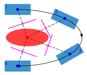
(a) $\gamma=0.5$

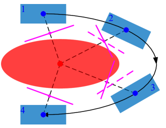
(b) $\gamma=0.75$

Figure 2: Positions of the proposed initial separating hyperplanes when weight factor $\gamma$ is set as 0.5 and 0.75, depending on the size of the obstacle. The controlled object $\mathcal{B}$ is denoted as a polygon, depicted in blue. The obstacle $\mathcal{O}$ is denoted as an ellipse, depicted in red. Centers of $\mathcal{B}$ and $\mathcal{O}$ are depicted in blue point and red point, respectively. The initial path is depicted in black solid line. The magenta lines in samples 1–4 are the initial separating hyperplanes. In (a), the size of $\mathcal{O}$ is smaller, we choose $\gamma=0.5$ to keep the hyperplane separating $\mathcal{B}$ from $\mathcal{O}$ in each sample, while in (b), $\gamma=0.75$ is set to keep the separating hyperplanes as far away from $\mathcal{O}$ as possible. Although the hyperplanes in samples 2 and 4 are not fully separating $\mathcal{B}$ from $\mathcal{O}$, such initialization may still help the solver quickly find the resulting separating hyperplanes in the neighborhood, i.e., starting from the solid lines, the solver may more easily find the magenta dotted lines.

VI-B Geometry-based initial guess

Since the planning OCP (2) is a non-convex optimization problem, good initialization in state variables, control variables, and auxiliary variables used to formulate collision avoidance constraints can improve the computational performance and the resulting solution quality. Much existing work has designed efficient initial guesses in state variables and control variables, e.g., Hybrid $\mathrm{A}^{\star}$ algorithm [1, 26]. Some researchers choose to initialize auxiliary variables by solving a convex optimization problem [26, 36]. However, it is noted that the number of auxiliary variables is very large, especially needed using the aforementioned dual formulations and Farkas’ Lemma, so this numerical optimization way is not efficient. Other researchers [1, 38] prefer to initialize auxiliary variables with constants, e.g., zero or a small value to avoid a singularity, but this way may affect solution quality on account of not being problem-dependent.

Owing to the proposed formulations using the hyperplane separation theorem, we propose a geometry-based method to initialize auxiliary variables. According to Theorem 1, when convex sets $\mathcal{B}_{m}$ and $\mathcal{O}_{n}$ are disjoint, i.e., $\mathcal{B}_{m}\cap\mathcal{O}_{n}=\emptyset$, there exists a separating hyperplane, which is described by auxiliary variables, e.g., $\boldsymbol{\lambda},\mu$ in formulation (13). Rather than initializing these auxiliary variables, as an alternative, we initialize the separating hyperplane from a view of geometry. It is done by finding a middle hyperplane between $\mathcal{B}_{m}$ and $\mathcal{O}_{n}$, i.e., let auxiliary variables be initialized with a coefficient vector describing the separating hyperplane which is orthogonal to the line crossing the sample on the initial path and the centroid of an obstacle, and crosses certain point between the sample and the centroid. An example of this initial separating hyperplane is illustrated in Fig 2. Because the initial guesses in auxiliary variables using the proposed geometry-based method can be obtained by calculating analytical solutions directly, it is simple and computationally efficient.

In the previous paragraph, we introduce a general method of how to initialize the separating hyperplanes, i.e., using an orthogonal hyperplane, but the geometry-based method is not limited to this. Because the initialization of the separating hyperplanes is highly problem-dependent, the initialization method should be carefully selected to optimize computational performance in various planning cases.

VII Applications

In this section, we show two applications of the proposed unified planning framework involving containing constraints and separating constraints. One case is autonomous parking in tractor-trailer vehicles in a limited moveable environment. The other case is car overtaking within narrow curved lanes. Additionally, in each case, comparisons with the state of the art on the same premise are done to illustrate the advantages of the proposed formulations.

VII-A Autonomous Parking for tractor-trailer vehicles

VII-A1 Problem description

Tractor-trailer vehicles are longer than standard cars, resulting in larger turning curvatures and a wider swept area, which makes their control difficult. The difficulty of parking is also significantly influenced by the parking geometry, whether it be parallel, angular, or perpendicular. Besides, in a limited nonconvex parking region, maintaining an acceptable safety distance from obstacles to prevent collisions poses a demanding task even for skilled drivers[8, 55], so it is an intractable issue for tractor-trailer vehicles parking within confined surroundings. Since the execution of reverse parking presents greater complexity in typical scenarios, autonomous reverse parking in tractor-trailer vehicles is studied by exploiting separating constraints (12) and containing constraints (16).

VII-A2 Case description

In the example of Fig. 3(a) and Fig. 3(b), the driving environment $\mathcal{W}$ is modeled by a convex polygon, depicted in green, denoted as $\mathcal{W}:=\left\{\boldsymbol{s}\in\mathbb{R}^{2}\mid P_{1}\boldsymbol{s}\leq\boldsymbol{p_{1}}\right\},$ where $P_{1}=[0,1,0,-1;1,0,-1,0]^{\top},\boldsymbol{p_{1}}=[10,10,10,6]^{\top}$. The obstacle $\mathcal{O}$ is modeled by a convex polygon, depicted in red solid. Let $V_{O}\in\mathbb{R}^{2\times 4}$ represent a matrix of vertices in $\mathcal{O}$, denoted as $V_{O}=\begin{bmatrix}7,7,-6,-6;-3,-10,-10,-3\end{bmatrix}$. The tractor-trailer vehicle $\mathcal{B}$ is modeled using a union of two convex polygons $\mathcal{B}_{1}$ and $\mathcal{B}_{2}$, depicted in magenta and blue. Polygons $\mathcal{B}_{1}$ and $\mathcal{B}_{2}$ are connected at the common articulated joint point. Because the position and orientation of the vehicle change, its set $\mathcal{B}_{i}(\boldsymbol{\xi})$ should be written to depend on the vehicle state $\boldsymbol{\xi}$, $i=1,2$. The matrix of vertices in $\mathcal{B}_{i}(\boldsymbol{\xi})$ is represented by $V_{i}(\boldsymbol{\xi})\in\mathbb{R}^{2\times 4}$. Matrix $V_{i}(\boldsymbol{\xi})$ can be obtained by the rotation and translation of the initial matrix as

$$V_{i}(\boldsymbol{\xi})=R_{i}(\boldsymbol{\xi})V_{i}(0)+\boldsymbol{T_{i}}(\boldsymbol{\xi})\boldsymbol{1}^{\top},$$ (21)

where $V_{i}(0)$ is denoted as the initial matrix, denoted as $V_{1}(0)=\begin{bmatrix}1.5,1.5,-0.5,-0.5;1,-1,-1,1\end{bmatrix}$, $V_{2}(0)=\begin{bmatrix}0.5,0.5,-5,-5;1,-1,-1,1\end{bmatrix}$. The rotation matrix is represented as $R_{i}(\boldsymbol{\xi})$. The translation vector is $\boldsymbol{T_{i}}(\boldsymbol{\xi})$. The collision avoidance requirements, i.e., $\mathcal{B}\cap\mathcal{O}=\emptyset$ and $\mathcal{B}\subset\mathcal{W}$ are approached by using the proposed (12) and (16), respectively.

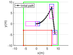
(a) Initial path

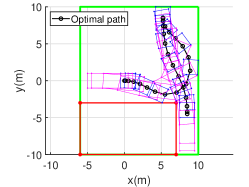
(b) Parking a tractor-trailer vehicle

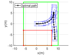
(c) Parking under one obstacle

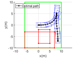
(d) Parking under two obstacles

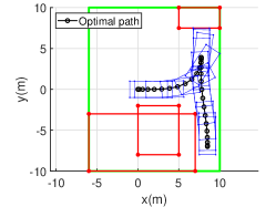
(e) Parking under three obstacles

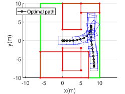
(f) Parking under four obstacles

Figure 3: Subplot (a) illustrates the initial path using piecewise polynomials. The interim position used to obtain an initial path is denoted as $[$7\text{\,}\mathrm{m}$,$7.5\text{\,}\mathrm{m}$]$. Subplot (b) shows the planned optimal path of a tractor-trailer vehicle. In (b), the starting state $\boldsymbol{\xi_{\mathrm{init}}}$ is $\begin{bmatrix}$0\text{\,}\mathrm{m}$,$0\text{\,}\mathrm{m}$,$0\text{\,}\mathrm{\SIUnitSymbolDegree}$,$0\text{\,}\mathrm{\SIUnitSymbolDegree}$,$0\text{\,}\mathrm{m}\mathrm{/}\mathrm{s}$,$0\text{\,}\mathrm{\SIUnitSymbolDegree}$\end{bmatrix}$. The ending state $\boldsymbol{\xi_{\mathrm{final}}}$ is $\begin{bmatrix}$8.5\text{\,}\mathrm{m}$,$-4.5\text{\,}\mathrm{m}$,$90\text{\,}\mathrm{\SIUnitSymbolDegree}$,$90\text{\,}\mathrm{\SIUnitSymbolDegree}$,$0\text{\,}\mathrm{m}\mathrm{/}\mathrm{s}$,$0\text{\,}\mathrm{\SIUnitSymbolDegree}$\end{bmatrix}$. Subplots (c)–(f) are the optimal paths of a single car under different obstacles. In (c)–(f), the starting state $\boldsymbol{\xi_{\mathrm{init}}}$ is $\begin{bmatrix}$0\text{\,}\mathrm{m}$,$0\text{\,}\mathrm{m}$,$0\text{\,}\mathrm{\SIUnitSymbolDegree}$,$0\text{\,}\mathrm{m}\mathrm{/}\mathrm{s}$,$0\text{\,}\mathrm{\SIUnitSymbolDegree}$\end{bmatrix}$. The ending state $\boldsymbol{\xi_{\mathrm{final}}}$ is $\begin{bmatrix}$8.5\text{\,}\mathrm{m}$,$-7\text{\,}\mathrm{m}$,$90\text{\,}\mathrm{\SIUnitSymbolDegree}$,$0\text{\,}\mathrm{m}\mathrm{/}\mathrm{s}$,$0\text{\,}\mathrm{\SIUnitSymbolDegree}$\end{bmatrix}$.

VII-A3 Vehicle model and objective function

The vehicle motion is described using a kinematic model, extended with a trailer [56, 57] as

$$\begin{array}[]{l}\dot{x}=v\cos(\theta_{1}),\\ \dot{y}=v\sin(\theta_{1}),\\ \dot{\theta_{1}}=v\tan(\delta)/L_{1},\\ \dot{\theta_{2}}=v\sin(\theta_{1}-\theta_{2})/L_{2},\\ \dot{v}=a,\\ \dot{\delta}=\omega,\end{array}$$ (22)

where $L_{1}=$1\text{\,}\mathrm{m}$$ and $L_{2}=$4.5\text{\,}\mathrm{m}$$ are wheelbases of the tractor and the trailer, respectively. The position of the tractor-trailer joint is identical to the vector $\left(x,y\right)$, and $\theta_{1}$, $\theta_{2}$ represent yaw angles of the tractor and the trailer with respect to the horizontal axle. The velocity and acceleration of the tractor-trailer joint are $v$ and $a$. The steering angle and the gradient of the steering angle of the tractor are denoted by $\delta$ and $\omega$, respectively. The state and control vectors can be summarized as

$$\begin{array}[]{c}\boldsymbol{\xi}=\begin{bmatrix}x&y&\theta_{1}&\theta_{2}&v&\delta\end{bmatrix}^{\top},\boldsymbol{u}=\begin{bmatrix}a&\omega\end{bmatrix}^{\top},\\ \end{array}$$ (23)

so the vehicle dynamics can be denoted as $\dot{\boldsymbol{\xi}}=f\left(\boldsymbol{\xi},\boldsymbol{u}\right)$. The feasible values of $\theta_{1},\theta_{2},v,\delta$ are limited to $|\theta_{1}|\leq$180\text{\,}\mathrm{\SIUnitSymbolDegree}$$, $|\theta_{2}|\leq$180\text{\,}\mathrm{\SIUnitSymbolDegree}$$, $|v|\leq\frac{5}{3.6}$\mathrm{m}\mathrm{/}\mathrm{s}^{2}$$, $|\delta|\leq 40$\mathrm{\SIUnitSymbolDegree}$$. The feasible inputs are given by $|a|\leq$1\text{\,}\mathrm{m}\mathrm{/}\mathrm{s}^{2}$$ and $|\omega|\leq$5\text{\,}\mathrm{\SIUnitSymbolDegree}\mathrm{/}\mathrm{s}^{2}$$. Specifically, the articulated joint angle at the tractor-trailer joint is limited using the constraint

$$|\theta_{1}-\theta_{2}|\leq 60$\mathrm{\SIUnitSymbolDegree}$.$$ (24)

In parking cases, we expect the autonomous vehicle to complete the parking maneuvers subjected to minimum traveling time. However, the parking duration, denoted as $t_{f}$, is not known in advance. To address this problem, We introduce a new independent variable $\tau\in[0,1]$, and express the time as $t=t_{f}\tau$, where $t_{f}\geq 0$ is a scalar optimization variable that needs to be added to the problem. Thus, the vehicle dynamics in (22) become a function of $\tau$ as

$$\frac{\mathrm{d}\boldsymbol{\xi}(\tau)}{\mathrm{d}\tau}=t_{f}f(\boldsymbol{\xi}(\tau),\boldsymbol{u}(\tau)).$$ (25)

Apart from the penalty on traveling time, the control input $a$ and $\omega$ should be small to yield smooth trajectories. Thus, a typical time-energy cost function in OCP (2) is formulated as

$$\underset{\boldsymbol{\xi},\boldsymbol{u},t_{f},(\cdot)}{\text{min}}t_{f}\left(r+\int_{0}^{1}\left\|\boldsymbol{u}\left(\tau\right)\right\|_{Q}^{2}\mathrm{d}\tau\right),$$ (26)

where $r$ is a penalty factor that trades the parking time with the rest of the cost. The notation $\left\|\cdot\right\|_{Q}^{2}$ represents squared Euclidean norm weighted by matrix $Q$. For the studied cases we choose $r=1,Q={\rm diag}(100,200)$.

The OCP (2) is generally reformulated as a discrete NLP problem that can be solved using off-the-shelf solvers. The whole region $[0,1]$ is discretized into ${k}_{f}+1$ parts, i.e., $1={k}_{f}\Delta\tau$, where $\Delta\tau$ is the sampling interval. Variable $\tau$ is replaced with $\tau={k}\Delta\tau$, where ${k}=0$, $\ldots$, ${k}_{f}$. Thus, the OCP (2) involving collision avoidance can be formulated as a discrete NLP problem

$$\underset{\boldsymbol{\xi},\boldsymbol{u},t_{f},(\cdot)}{\text{min}} \ rt_{f}+\sum_{k=0}^{k_{f}-1}\tilde{\ell}(\boldsymbol{u}(k),t_{f})$$ (27a)

s.t. $$\boldsymbol{\xi}(0)=\boldsymbol{\xi_{\mathrm{init}}},\ \boldsymbol{\xi}(k_{\mathrm{f}})=\boldsymbol{\xi_{\mathrm{final}}},$$ (27b)

$$\boldsymbol{\xi}(k+1)=\tilde{f}\left(\boldsymbol{\xi}(k),\boldsymbol{u}(k),t_{f}\right),$$ (27c)

$$\boldsymbol{\xi}(k)\in\mathcal{X},\ \boldsymbol{u}(k)\in\mathcal{U},$$ (27d)

$$(\ref{eq12}),(\ref{eq28}),$$ (27e)

where symbol $(\cdot)$ is a shorthand notation for decision variables that need to be added to the vector of existing optimization variables, e.g., $\mu$ in formulation (12). Symbol $\tilde{f}$ denotes the discretized model dynamics of (25) and symbol $\tilde{\ell}$ is the discretized form of the state cost $t_{f}\left\|\boldsymbol{u}\left(\tau\right)\right\|_{Q}^{2}$ in function (26). In the simulation, the 4-th order Runge-Kutta method [38] is chosen to express the discretized $\tilde{\ell}$ and $\tilde{f}$.

Since the resulting NLP (27) is nonconvex, multiple local solutions exist depending on different initial guesses. An initial guess in the neighborhood of a local solution is more likely to cause the NLP solver to return that local solution. In a reverse parking scenario, we use piecewise polynomials to initialize states $x,y$. In the example of Fig 3(a) and Fig 3(b), we expect that the vehicle parks into the garage by reversing only once, so the initial guess in positions is defined by using a second-order polynomial from the starting position to an interim position and a linear function from the interim position and ending position (see Fig. 3(a)). The yaw angle is initialized as the angle between a line tangent to the polynomial trajectory at each sample and the horizontal axle. Other states and inputs are initialized as zero. As mentioned in Section VI-B, let the initial separating hyperplane, which is used to initialize auxiliary variables $\boldsymbol{\lambda}$, $\mu$ in formulation (12), be initialized with the hyperplane orthogonal to the line crossing the sample on the polynomial trajectory and the centroid of an obstacle. In the example, we set $\gamma=0.75$ to position the initial hyperplane near the vehicle. Finding an initial guess of parking time $t_{f}$ is challenging and highly problem-dependent, so for this reverse parking case, we use an estimated value of $50\text{\,}\mathrm{s}$ to warmly start $t_{f}$ [3, 26].

Simulations are conducted in MATLAB R2020a and executed on a laptop with AMD R7-5800H CPU at 3.20 GHz and 16GB RAM. Since we use a multiple-shooting approach, the problem is formulated as a collection of $k_{\mathrm{f}}$ phases. In this case, $k_{\mathrm{f}}=30$ phases are chosen. The problems are then implemented using CasADi [53]. The resulting discrete NLP (27) is solved using solver IPOPT [54].

VII-A4 Solution

Simulation results are visually interpreted in Fig. 3(b). It can be seen that the planned optimal path is smooth and collision-free. Vertices of polygons $\mathcal{B}_{1}$ and $\mathcal{B}_{2}$ do not enter into obstacle $\mathcal{O}$, and vertices of $\mathcal{O}$ are prevented from passing the edges of $\mathcal{B}_{1}$ and $\mathcal{B}_{2}$. It can be noticed that since the parking environment $\mathcal{W}$ is limited, the vehicle keeps close to the environment boundaries to allow larger turning curvatures, but it is contained within $\mathcal{W}$ all the time. In the resulting solution, the vehicle conducts a reverse behavior to adjust its pose to enter into the confined parking place. Additionally, the implementing time to solve problem (27) using IPOPT is $2.264\text{\,}\mathrm{s}$ and the resulting parking duration is $69.89\text{\,}\mathrm{s}$.

TABLE II: The result of computational cost by using different methods

Performance	Algorithms	One	Two	Three	Four
Number of auxiliary variables to be optimized	proposed	306	396	486	576
	[3]	456	696	936	1176
	[7]	456	696	936	1176
Solving time (s)	proposed	1.92	1.336	2.239	3.048
	[3]	2.03	3.008	20.086	19.977
	[7]	4.098	4.66	18.449	18.701
Objective value	proposed	73.45	73.45	75.13	75.13
	[3]	73.45	73.45	77.7021	75.13
	[7]	73.45	73.45	75.13	75.13
$t_{f}$ (s)	proposed	52.56	52.56	51.55	51.55
	[3]	52.56	52.56	54.17	51.55
	[7]	52.56	52.56	51.55	51.55

• The red values represent the obtained other local solutions based on the same initial guess.

VII-A5 Comparisons in problem size

This part is used to support the advantage of improving computational performance on account of admitting a reduced problem size compared to existing approaches. It is noted that the nonconvex parking problem (27) may converge to multiple local solutions even if based on the same initial guess. Indeed, a vehicle may take infinitely many paths to reach the goal, especially for a tractor-trailer vehicle with more states. However, we expect to compare the computational performance of the proposed algorithms with the state of the art under the condition of converging to the same local solution, so we design a new case of a single-car parking problem. Here, we use a simplified vehicle model of (22), with $L_{1}=2.6$. The vehicle dynamics is modelled with the reduced state vector $\boldsymbol{\xi}=\left[x,y,\theta_{1},v,\delta\right]^{\top}$ and control vector $\boldsymbol{u}\left(s\right)=\left[a,\omega\right]^{\top}$. Let the initial matrix $V_{1}(0)$ be denoted as $V_{1}(0)=\begin{bmatrix}3.6,3.6,-1,-1;1,-1,-1,1\end{bmatrix}$.

To keep the same premise of the NLP configuration, the initial guess in states $x,y,\theta_{1}$ is a linear function (starting from the beginning and ending at the final values). The rest of the states and inputs are set as zero. Let $\boldsymbol{\lambda}$ in formulation (12) be initialized with a positive value vector to prevent a singularity and $\mu$ be set to zero. We conduct numerical experiments by comparing formulation (12) with the formulations in Proposition 3 of [3] and in Section III-A-2 of [7]. Others remain unchanged in NLP (27).

We design four scenarios to test collision avoidance with different placement of obstacles. The resulting optimal trajectories are illustrated in Fig. 3(c)–(f). The computational results are shown in Table II. It can be seen that these planned trajectories are collision-free and smooth. Apart from the scenario of three obstacles, the solver converges to the same local solution using different methods. Alternatively, we can verify the comparison results in the other three scenarios. The primal observation in Table II is the least number of auxiliary variables by exploiting the proposed formulation (12) in each scenario, which illustrates that using the proposed formulation (12) shows a considerable reduction in the problem size of NLP formulations compared to the other two existing formulations. From Fig. 3(c) to Fig. 3(f), we increase another three polygonal obstacles orderly, and it can be seen that the number of variables experiences a relatively low increase using the proposed formulation (12) but a sharp increase using formulations in [3, 7]. In Fig. 3(c)–(f), our method needs $3\times k_{f}=90$ auxiliary variables ($\boldsymbol{\lambda}\in\mathbb{R}^{2},\mu\in\mathbb{R}$ in formulation (12)) per obstacle. On the contrary, existing formulations in [3, 7] identify variables associated with the edges of a vehicle and an obstacle, depending on the number of the total edges of the vehicle and all obstacles, i.e., adding $(4+4)\times k_{f}=240$ auxiliary variables per obstacle. The comparison of needed additional variables states that when the number of edges of each obstacle increases, more variables are needed to formulate constraints of [3, 7], while the number of variables by the proposed formulation (12) remains unchanged. Besides, it can be seen that as more obstacles are considered, it takes more time to solve an NLP. In each scenario, since the problem size using the proposed algorithm is smaller, solvers can converge to the same local optimums faster, which shows that the proposed method is more efficient compared with other algorithms.

VII-B Overtaking in curved lanes

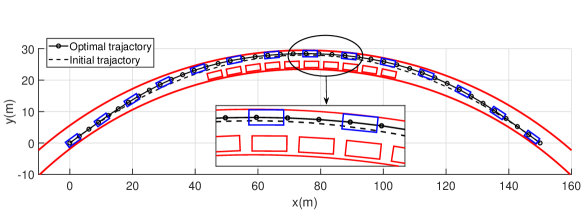
(a) The planning optimal trajectory in curved lanes

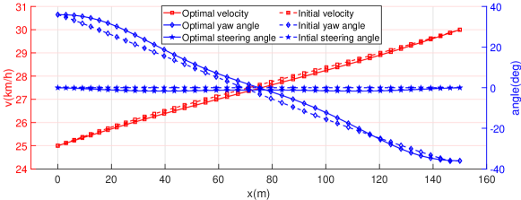
(b) The resulting states corresponding with the optimal trajectory

Figure 4: Results in the optimal trajectory and states in variable scenarios. In subplot (a), the curved lane is surrounded by two curves depicted in red solid. The boundary of obstacle $\mathcal{O}_{1}$ is denoted as the inner red curve. Positions of moving obstacle $\mathcal{O}_{2}$ are illustrated using red polygons. Positions of the overtaking process of the ego vehicle $\mathcal{B}$ are illustrated using blue polygons. In this scenario, the ego vehicle $\mathcal{B}$ will overtake the leading obstacle $\mathcal{O}_{2}$ in the constrained curved lane. The starting state $\boldsymbol{\xi_{\mathrm{init}}}$ is $\begin{bmatrix}$0\text{\,}\mathrm{m}$,$0\text{\,}\mathrm{m}$,$36\text{\,}\mathrm{\SIUnitSymbolDegree}$,$25\text{\,}\mathrm{k}\mathrm{m}\mathrm{/}\mathrm{h}$,$0\text{\,}\mathrm{\SIUnitSymbolDegree}$\end{bmatrix}$. The ending state $\boldsymbol{\xi_{\mathrm{final}}}$ are $\begin{bmatrix}$150\text{\,}\mathrm{m}$,$0\text{\,}\mathrm{m}$,$-36\text{\,}\mathrm{\SIUnitSymbolDegree}$,$30\text{\,}\mathrm{k}\mathrm{m}\mathrm{/}\mathrm{h}$,$0\text{\,}\mathrm{\SIUnitSymbolDegree}$\end{bmatrix}$. The initial path and the planned optimal path are depicted in subplot (a). The designed initial states and the resulting states are depicted in subplot (b).

VII-B1 Problem description

It is common for a vehicle to drive in curved lanes, e.g., trucks safely traveling on mountain roads and cars racing in closed-loop tracks [35, 51, 52]. These vehicles are expected to reside within a narrow curved lane, not colliding with moving obstacles. Typically, it is difficult to overtake a moving obstacle for intelligent vehicles in a narrow curved environment, especially for a long-size vehicle. To approach this issue, we use separating constraints (12), (14) and containing constraints (16) in the proposed planning framework.

VII-B2 Case description

In the example of Fig. 4(a) and Fig. 4(e), the driving environment $\mathcal{W}$ is modeled by an ellipse, depicted in outer red solid line, denoted as $\mathcal{W}:=\left\{\boldsymbol{s}\in\mathbb{R}^{2}\mid\left(\boldsymbol{s}-\boldsymbol{e_{1}}\right)^{\top}E_{1}\left(\boldsymbol{s}-\boldsymbol{e_{1}}\right)\leq 1\right\},$ where $E_{1}=\text{diag}(1/129.5^{2},1/129.5^{2})$, $\boldsymbol{e_{1}}=[75,-100]^{\top}$. The obstacle $\mathcal{O}_{1}$ is modeled by an ellipse denoted as $\mathcal{O}_{1}:=\left\{\boldsymbol{s}\in\mathbb{R}^{2}\mid\left(\boldsymbol{s}-\boldsymbol{e_{2}}\right)^{\top}E_{2}\left(\boldsymbol{s}-\boldsymbol{e_{2}}\right)\leq 1\right\}$, where $E_{2}=\text{diag}(1/123.5^{2},1/123.5^{2})$, $\boldsymbol{e_{2}}=[75,-100]^{\top}$. It is illustrated by the inner red solid line in the figure. It can be noticed that the curved lane is constructed with an intersection of ellipse $\mathcal{W}$ and ellipse $\mathcal{O}_{1}$, i.e., $\mathcal{W}\cap\mathcal{O}_{1}$. Another moving obstacle is denoted as a polygon $\mathcal{O}_{2}$ of size $$4.6\text{\,}\mathrm{m}$\times$2\text{\,}\mathrm{m}$$. We assume obstacle $\mathcal{O}_{2}$ moves slowly in a predefined path, which is defined as a uniform circular motion with $1.32\text{\,}\mathrm{\SIUnitSymbolDegree}\mathrm{/}\mathrm{s}$. It is illustrated by a red solid polygon in Fig. 4(a). The ego vehicle $\mathcal{B}$ is modeled as a polygon of the same size as $\mathcal{O}_{2}$, depicted in blue. The matrix of vertices in $\mathcal{B}(\boldsymbol{\xi})$ is represented by $V(\boldsymbol{\xi})\in\mathbb{R}^{2\times 4}$. In this overtaking planning problem, the ego vehicle should reside in the curved lane and not collide with obstacles, represented as $\mathcal{B}\cap\mathcal{O}_{1}=\emptyset$, $\mathcal{B}\cap\mathcal{O}_{2}=\emptyset$, and $\mathcal{B}\subset\mathcal{W}$, which are approached by using the proposed formulations (14), (12), and (16).

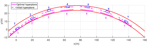
(a) Tangent hyperplanes used to initialize variables in constraint (14)

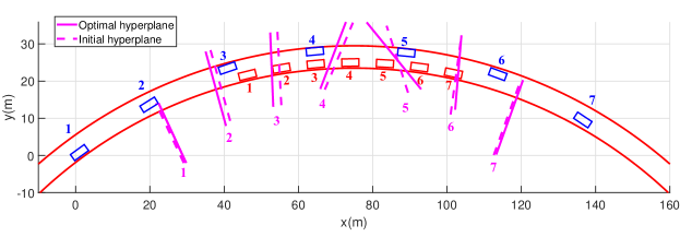
(b) Orthogonal hyperplanes used to initialize variables in constraint (12)

Figure 5: The hyperplanes in different samples. The hyperplanes to initialize auxiliary variables in constraints (14) and (12) are depicted in magenta dotted lines of (a) and (b), respectively. The resulting hyperplanes are depicted in magenta solid lines. In (b) positions of moving obstacle $\mathcal{O}_{2}$ are depicted in red polygons. Subplots (a)–(b) illustrate positions of the initial hyperplanes and resulting hyperplanes in seven samples. It can be seen that in each sample the initial hyperplane is close to the resulting hyperplane and the resulting hyperplane can separate the vehicle from obstacle $\mathcal{O}_{1}$ in (a) and separate the vehicle from moving obstacle $\mathcal{O}_{2}$ in (b).

VII-B3 Vehicle model and cost function

As Section VII-A5 does, we use a simplified vehicle model of (22), i.e., with the reduced state vector $\boldsymbol{\xi}=\left[x,y,\theta,v,\delta\right]^{\top}$ and control vector $\boldsymbol{u}\left(s\right)=\left[a,\omega\right]^{\top}$, where $\theta$ represents the yaw angle with respect to the horizontal axle. The feasible values of $\theta,v,\delta$ are limited to $|\theta|\leq$85\text{\,}\mathrm{\SIUnitSymbolDegree}$$, $\frac{5}{3.6}$\mathrm{m}\mathrm{/}\mathrm{s}^{2}$\leq v\leq\frac{60}{3.6}$\mathrm{m}\mathrm{/}\mathrm{s}^{2}$$, $|\delta|\leq 45$\mathrm{\SIUnitSymbolDegree}$$. Additionally, the feasible inputs are given by $$-1\text{\,}\mathrm{m}\mathrm{/}\mathrm{s}^{2}$\leq a\leq$2\text{\,}\mathrm{m}\mathrm{/}\mathrm{s}^{2}$$ and $|\omega|\leq$5\text{\,}\mathrm{\SIUnitSymbolDegree}\mathrm{/}\mathrm{s}^{2}$$.

In this overtaking case, we expect the vehicle to drive smoothly to a target position subject to a given time $t_{f}$. A discretization procedure can then similarly be applied as proposed in Section VII-A3, i.e., the given time $t_{f}$ is divided into ${k}_{f}+1$ parts. In the objective function, the control inputs $a$ and $\omega$ are penalized as $\sum_{k=0}^{k_{f}-1}\left\|\boldsymbol{u}\left(k\right)\right\|_{Q}^{2}$, with $Q={\rm diag}(10,20)$. Thus, the OCP (2) is formulated as the NLP

$$\underset{\boldsymbol{\xi},\boldsymbol{u},(\cdot)}{\text{min}} \ \sum_{k=0}^{k_{f}-1}\left\|\boldsymbol{u}\left(k\right)\right\|_{Q}^{2}$$ (28a)

s.t. $$\boldsymbol{\xi}(0)=\boldsymbol{\xi_{\mathrm{init}}},\ \boldsymbol{\xi}(k_{\mathrm{f}})=\boldsymbol{\xi_{\mathrm{final}}},$$ (28b)

$$\boldsymbol{\xi}(k+1)=\tilde{f}\left(\boldsymbol{\xi}(k),\boldsymbol{u}(k)\right),$$ (28c)

$$\boldsymbol{\xi}(k)\in\mathcal{X},\ \boldsymbol{u}(k)\in\mathcal{U},$$ (28d)

$$(\ref{eq12}),(\ref{eq21}),(\ref{eq28}),$$ (28e)

where symbol $\tilde{f}$ denotes the discretized symbol of vehicle model (22) with removing state $\theta_{2}$ related to the trailer. The 4-th order Runge-Kutta method is used to express the state evolution of (28c).

The 4-th order polynomial function is applied to generate a trajectory as the initial guesses [58, 59] in states $(x,y,\theta)$ . The initial guess for $v$ is a linear function from the initial to the final value. The rest of the states and inputs are set as zero. Let the initial separating hyperplane, which is used to initialize auxiliary variables $\boldsymbol{\lambda}$, $\mu$ in formulation (14), be initialized with the hyperplane tangent to the polynomial trajectory at each sample. Likewise in the parking case, let the hyperplane, which is to initialize $\boldsymbol{\lambda}$, $\mu$ in formulation (12), be orthogonal to the line crossing the sample on the polynomial trajectory and the centroid of an obstacle, and $\gamma=0.5$ is set. In this overtaking case, the horizon time is set to $21\text{\,}\mathrm{s}$ and $k_{\mathrm{f}}=40$. Other NLP configurations are the same as that of the parking case.

VII-B4 Solution

The optimal trajectory and states are visually interpreted in Fig. 4. The primary observation in Fig. 4(a) is that the resulting optimal path is smooth and collision-free. In this overtaking case, since a higher speed is acquired, a larger turning radius of the car is needed. Because this curved lane is narrow, it can be seen that the vehicle keeps on close to the environment boundaries when driving during [$40\text{\,}\mathrm{m}$,$100\text{\,}\mathrm{m}$], while each vertex of the vehicle does not cross the boundaries. The proposed containing constraint (16) contributes to this. Additionally, the vehicle completes the overtaking task subject to a given time, not colliding with the moving obstacle $\mathcal{O}_{2}$, and also during this whole process the vehicle does not enter into obstacle $\mathcal{O}_{2}$. Another observation in Fig. 4(a)–Fig. 4(b) is that the resulting optimal paths and states are close to the designed initial guesses, indicating that the given initial guesses can improve the efficiency and solution quality in solving the nonconvex NLP (28). Additionally, from the state profile of Fig. 4(b), the steering angle, the velocity, and the yaw angle of the vehicle vary steadily during the traveling process and achieve the expected target states.

VII-B5 Comparisons in initializing auxiliary variables

To investigate the computational cost of the proposed formulations (12) and (14) when initialized differently, comparative experiments are conducted under existing initialization methods in [1] and the proposed geometry-based methods, respectively. The existing method initializes $\boldsymbol{\lambda}$, in formulations (12) and (14) of NLP (28), with a positive value to prevent a singularity and $\mu$ is set to zero. The proposed method uses an orthogonal hyperplane to initialize the auxiliary variables in formulation (12) and a tangent hyperplane to initialize the auxiliary variables in formulation (14). Other configurations of NLP (28) remain unchanged.

Fig. 5 illustrates the proposed geometry-based initial guesses. It can be seen that the designed initial hyperplane in each sample is in the neighborhood of the resulting separating hyperplane, showing that the auxiliary variables related to constraints (12) and (14) have been well initialized. This is beneficial to solve the nonconvex NLP (28), which is supported in Table III showing the computational results using different initialization methods. From Table III, though using different initial guesses the resulting optimal solutions are exactly the same, i.e., the objective value is 0.907 and the TS is 0.168. However, the result of solving time shows that the proposed geometry-based guesses lead to the less computation time than the existing guesses, especially when initializing the variables in constraints (12). This illustrates the computational advantages of our methods, which are highly beneficial for efficient collision avoidance.

TABLE III: Results in computational effort using different initial guesses.

Ways to initialize auxiliary variables in (12) and (21)	Objective value	TS1	Solving time (s)
Proposed to (12) & Proposed to (21)	0.907	0.168	1.3622
Existing to (12) & Proposed to (21)	0.907	0.168	8.314
Proposed to (12) & Existing to (21)	0.907	0.168	2.132

• The value $\mathrm{TS}=\sum_{{k}=0}^{{k}_{f}-1}\left(a(k)^{2}+\omega(k)^{2}\right)$ is calculated to double check if the NLP (28) converges to the same local solution under a same objective value.

• The bold value denotes the least solving time.

VIII Conclusion and future work

This article investigates optimization-based methods aiming to achieve exact collision avoidance of controlled objects. In the proposed unified planning framework, we formulate smooth collision avoidance constraints by utilizing the hyperplane separation theorem to separate a pair of convex sets, and S-procedure and geometrical methods to contain a convex set inside another convex set. The proposed collision avoidance formulations are highly beneficial for reducing an NLP problem size and efficient initialization of auxiliary variables, which admits an improved computational performance compared to the state of the art.

Based on the proposed planning framework, the next work will first focus on the research of the uncertainty from localization errors, system delay, etc. Additionally, since collision formulations using dual methods in [3] (with higher complexity than the proposed collision formulations using the hyperplane separation theorem) have successfully been implemented in real-time [36] and even in real-world scenarios [60, 61], it is possible to execute the proposed methods in real-time by sequential quadratic programming implementations [62, 63]. Real-time control implementation of the proposed method will also be considered in future studies.

Appendix A Extensions of separating constraints

A-A Hyperplane with bounded slope or displacement

In Proposition 3, Proposition 4, and Proposition 5, we propose using $N+1$ auxiliary variables to describe a separating hyperplane. The three propositions are sufficient and necessary conditions of $\mathcal{B}_{m}\cap\mathcal{O}_{n}=\emptyset$. In principle, it is possible to use fewer variables to obtain sufficient conditions of $\mathcal{B}_{m}\cap\mathcal{O}_{n}=\emptyset$. For instance, consider Proposition 3 under $N=2$. According to the proposition, 3 auxiliary variables are needed to construct a hyperplane as

$$\mathcal{B}_{m}\cap\mathcal{O}_{n}=\emptyset\iff\exists\boldsymbol{\lambda}\in\mathbb{R}^{2},\mu\in\mathbb{R}:$$ (29)

$$\begin{array}[]{c}\boldsymbol{\lambda}^{\top}V_{P_{1}}\geq\mu\boldsymbol{1}^{\top},\boldsymbol{\lambda}^{\top}V_{P_{2}}\leq\mu\boldsymbol{1}^{\top},\left\|\boldsymbol{\lambda}\right\|>0.\end{array}$$

In certain cases, it is possible to use only 2 auxiliary variables. For e.g., if it is known that $\mu\neq 0$, the inequalities can be normalized by $\mu$ and a sufficient condition of $\mathcal{B}_{m}\cap\mathcal{O}_{n}=\emptyset$ can be formulated as

$$\mathcal{B}_{m}\cap\mathcal{O}_{n}=\emptyset\ \Longleftarrow\ \exists\boldsymbol{\lambda}\in\mathbb{R}^{2}:$$ (30)

$$\begin{array}[]{c}\boldsymbol{\lambda}^{\top}V_{P_{1}}\geq\boldsymbol{1}^{\top},\boldsymbol{\lambda}^{\top}V_{P_{2}}\leq\boldsymbol{1}^{\top},\left\|\boldsymbol{\lambda}\right\|>0.\end{array}$$

Alternatively, if it is known that both horizontal and vertical hyperplane slopes are not occurring in the same problem, then one of the $\boldsymbol{\lambda}$ is not zero and the inequality can be normalized with that value. For e.g., such a condition can be written as

$$\mathcal{B}_{m}\cap\mathcal{O}_{n}=\emptyset\ \Longleftarrow\ \exists\lambda\in\mathbb{R},\mu\in\mathbb{R}:$$ (31)

$$\begin{array}[]{c}\begin{bmatrix}\lambda&1\end{bmatrix}V_{P_{1}}\geq\mu\boldsymbol{1}^{\top},\begin{bmatrix}\lambda&1\end{bmatrix}V_{P_{2}}\leq\mu\boldsymbol{1}^{\top},\lambda^{2}>0.\end{array}$$

Thus, using fewer variables can simplify the Proposition 3, Proposition 4, and Proposition 5, which can further reduce problem size and computational load.

A-B A point-mass controlled object

Apart from the investigation of collision avoidance between polytopes and ellipsoids in this article, the hyperplane separation theorem can readily be applied to other compact sets. For instance, sometimes the controlled object $\mathcal{B}$ is regarded as a point-mass system. Let the position of a point $p$ be denoted as $\boldsymbol{p}\in\mathbb{R}^{N}$. Let set $\mathcal{O}_{n}$ be denoted using polytope $\mathcal{P}(P,\boldsymbol{p},\boldsymbol{s})$ as (3). Then,

$$p\cap\mathcal{O}_{n}=\emptyset\iff\exists\boldsymbol{\lambda}\in\mathbb{R}^{N},\mu\in\mathbb{R}:$$ (32)

$$\begin{array}[]{c}\boldsymbol{\lambda}^{\top}\boldsymbol{p}\geq\mu,\boldsymbol{\lambda}^{\top}V_{P}\leq\mu\boldsymbol{1}^{\top},\left\|\boldsymbol{\lambda}\right\|>0.\end{array}$$

In formulation (32), the number of additional variables i.e., $\boldsymbol{\lambda},\mu$, does not depend on the complexity of polytope $\mathcal{O}_{n}$, so formulation (32) also admits a reduced problem size compared to formulations in Proposition 1 of [3] and Section III-A-1 of [7].

It is possible to even further reduce the number of variables to formulate (32). The hyperplane for separation can be attached to the vehicle point $p$, i.e., $\boldsymbol{\lambda}^{\top}\boldsymbol{p}=\mu$, and a sufficient condition of $p\cap\mathcal{O}_{n}=\emptyset$ can be formulated as

$$p\cap\mathcal{O}_{n}=\emptyset\ \Longleftarrow \ \exists\boldsymbol{\lambda}\in\mathbb{R}^{N}:$$ (33)

$$\begin{array}[]{c}\boldsymbol{\lambda}^{\top}V_{P}\leq\boldsymbol{\lambda}^{\top}\boldsymbol{p}\boldsymbol{1}^{\top},\left\|\boldsymbol{\lambda}\right\|>0.\end{array}$$

References

- [1] C. Dietz, S. Albrecht, A. Nurkanović and M. Diehl, ”Efficient Collision Modelling for Numerical Optimal Control,” in Proc. Eur. Control Conf. (ECC), Bucharest, Romania, pp. 1-7, 2023.
- [2] J. Karlsson, N. Murgovski, and J. Sjoberg, ”Computationally Efficient Autonomous Overtaking on Highways,” IEEE Trans. Intell. Transp. Syst., vol. 21, no. 8, pp. 3169-3183, 2020.
- [3] X. Zhang, A. Liniger, and F. Borrelli, ”Optimization-Based Collision Avoidance,” IEEE Trans. Contr. Syst. Technol., vol. 29, no. 3, pp. 972-983, 2021.
- [4] J. Schulman et al., ”Motion planning with sequential convex optimization and convex collision checking,” Int. J. Robot. Autom., vol. 33, no. 9, pp. 1251-1270, 2014.
- [5] V. Sunkara, A. Chakravarthy and D. Ghose, ”Collision Avoidance of Arbitrarily Shaped Deforming Objects Using Collision Cones,” IEEE Robot. Autom. Lett., vol. 4, no. 2, pp. 2156-2163, 2019.
- [6] S. Haddadin, A. De Luca and A. Albu-Schäffer, ”Robot Collisions: A Survey on Detection, Isolation, and Identification,” IEEE Trans. Robot., vol. 33, no. 6, pp. 1292-1312, 2017.
- [7] S. Helling and T. Meurer, ”Dual Collision Detection in Model Predictive Control Including Culling Techniques,” IEEE Trans. Control. Syst. Technol., early access, 2023, doi: 10.1109/TCST.2023.3259822.
- [8] B. Li et al., ”Tractor-Trailer Vehicle Trajectory Planning in Narrow Environments With a Progressively Constrained Optimal Control Approach,” IEEE Trans. Intell. Veh., vol. 5, no. 3, pp. 414-425, 2020.
- [9] J. Schulman et al., ”Motion planning with sequential convex optimization and convex collision checking,” Int. J. Robot. Autom., vol. 33, no. 9, pp. 1251-1270, 2014.
- [10] P.F. Lima, ”Optimization-based motion planning and model predictive control for autonomous driving: With experimental evaluation on a heavy-duty construction truck,” Ph.D. dissertation, KTH Royal Institute of Technology, 2018.
- [11] J. Zhou, B. Olofsson and E. Frisk, ”Interaction-Aware Motion Planning for Autonomous Vehicles with Multi-Modal Obstacle Uncertainty Predictions,” IEEE Tran. Intell. Veh., early access, 2023, doi:10.1109/TIV.2023.3314709.
- [12] J. Zhou, B. Olofsson and E. Frisk, ”Interaction-Aware Moving Target Model Predictive Control for Autonomous Vehicles Motion Planning,” in Proc. Eur. Contr. Conf. (ECC), London, United Kingdom, pp. 154-161, 2022.
- [13] J. Hu, H. Zhang, L. Liu, X. Zhu, C. Zhao and Q. Pan, ”Convergent Multiagent Formation Control With Collision Avoidance,” IEEE Trans. Robot., vol. 36, no. 6, pp. 1805-1818, 2020.
- [14] D. Ioan, I. Prodan, S. Olaru, F. Stoican, and S. Niculescu, ”Mixed-integer programming in motion planning,” Annu. Rev. Contr., vol. 51, pp. 65-87, 2021.
- [15] I. E. Grossmann, ”Review of Nonlinear Mixed-Integer and Disjunctive Programming Techniques,” Optim. Eng., vol. 3, pp. 227–252, 2002.
- [16] S. M. LaValle planning algorithms. Cambridge University Press. 2006.
- [17] R. Deits and R. Tedrake, ”Efficient mixed-integer planning for UAVs in cluttered environments,” in Proc. IEEE Int. Conf. Robot. Autom. (ICRA), Seattle, WA, USA, pp. 42-49, 2015.
- [18] D. Mellinger, A. Kushleyev and V. Kumar, ”Mixed-integer quadratic program trajectory generation for heterogeneous quadrotor teams,” in Proc. IEEE Int. Conf. Robot. Autom. (ICRA), Saint Paul, MN, USA, pp. 477-483, 2012.
- [19] I. Prodan, F. Stoican, S. Olaru and S.I. Niculescu, Mixed-Integer Representations in Control Design Mathematical Foundations and Applications. Springer. 2015.
- [20] J. P. Vielma, ”Mixed Integer Linear Programming Formulation Techniques,” Siam. Rev., vol. 57, no. 1, pp. 3–57, 2015.
- [21] X. Wang, M. Kloetzer, C. Mahulea and M. Silva, ”Collision avoidance of mobile robots by using initial time delays,” in Proc. IEEE Conf. Decis. Control (CDC), Osaka, Japan, pp. 324-329, 2015.
- [22] I. Haghighi, S. Sadraddini and C. Belta, ”Robotic swarm control from spatio-temporal specifications,” in Proc. IEEE Conf. Decis. Control (CDC), Las Vegas, NV, USA, pp. 5708-5713, 2016.
- [23] J. Karlsson, N. Murgovski and J. Sjoberg, ”Comparison between mixed-integer and second order cone programming for autonomous overtaking,” in Proc. Eur. Control Conf. (ECC), Limassol, Cyprus, pp. 386-391, 2018.
- [24] F. Molinari, N. N. Anh, and L. Del Re, ”Efficient mixed integer programming for autonomous overtaking,” in Proc. Am. Control Conf. (ACC), Seattle, WA, USA, pp. 2303-2308, 2017.
- [25] H. P. Williams, Model Building in Mathematical Programming. Wiley. 2013.
- [26] X. Zhang, A. Liniger, A. Sakai and F. Borrelli, ”Autonomous Parking Using Optimization-Based Collision Avoidance,” ” in Proc. IEEE Conf. Decis. Contr. (CDC), Miami, FL, USA, pp. 4327-4332, 2018.
- [27] I. Ballesteros-Tolosana, S. Olaru, P. Rodriguez-Ayerbe, G. Pita-Gil and R. Deborne, ”Collision-free trajectory planning for overtaking on highways,” in Proc. IEEE Conf. Decis. Contr. (CDC), Melbourne, VIC, Australia, pp. 2551-2556, 2017.
- [28] Rubens J. M. Afonso, Roberto K. H. Galvão and K. H. Kienitz, ”Reduction in the number of binary variables for inter-sample avoidance in trajectory optimizers using mixed-integer linear programming,” Int. J. Robust Nonlinear Control., vol. 26, pp. 3662–3669, 2016.
- [29] F. Stoican, I. Prodan and S. Olaru, ”Hyperplane arrangements in mixed-integer programming techniques. Collision avoidance application with zonotopic sets,” in Proc. Eur. Control Conf. (ECC), Zurich, Switzerland, pp. 3155-3160, 2013.
- [30] A. Ganesan, S. Gros, and N. Murgovski, ”Numerical Strategies for Mixed-Integer Optimization of Power-Split and Gear Selection in Hybrid Electric Vehicles,” IEEE Trans. Intell. Transp. Syst., vol. 24, no. 3, pp. 3194-3210, 2023.
- [31] C. Kirches, Fast Numerical Methods for Mixed-Integer Nonlinear Model-Predictive Control. Springer. 2010.
- [32] H. Febbo, J. Liu, P. Jayakumar, J. L. Stein and T. Ersal, ”Moving obstacle avoidance for large, high-speed autonomous ground vehicles,” in Proc. Am. Control Conf. (ACC), Seattle, WA, USA, pp. 5568-5573, 2017.
- [33] U. Rosolia, S. De Bruyne, and A. G. Alleyne, “Autonomous vehicle control: A nonconvex approach for obstacle avoidance,” IEEE Trans. Control. Syst. Technol., vol. 25, no. 2, pp. 469–484, 2016.
- [34] M. Geisert and N. Mansard, ”Trajectory Generation for Quadrotor Based Systems using Numerical Optimal Control, ” in Proc. IEEE Int. Conf. Robot. Autom. (ICRA), Stockholm, Sweden, pp. 2958-2964, 2016.
- [35] J. Zeng, B. Zhang, and K. Sreenath, “Safety-critical model predictive control with discrete-time control barrier function,” in Proc. Am. Control Conf. (ACC), New Orleans, LA, USA, pp. 3882–3889, 2021.
- [36] A. Thirugnanam, J. Zeng and K. Sreenath, ”Safety-Critical Control and Planning for Obstacle Avoidance between Polytopes with Control Barrier Functions, ” in Proc. IEEE Int. Conf. Robot. Autom. (ICRA), Philadelphia, PA, USA, pp. 286-292, 2022.
- [37] J. Fan, N. Murgovski, and J. Liang, ” Efficient collision avoidance for autonomous vehicles in polygonal domains,” 2023, arXiv:2308.09103v2. Available: https://arxiv.org/abs/2308.09103.
- [38] J. Guthrie, ”A Differentiable Signed Distance Representation for Continuous Collision Avoidance in Optimization-Based Motion Planning,” in Proc. IEEE Conf. Decis. Control (CDC), Cancun, Mexico, pp. 7214-7221, 2022.
- [39] Y. Zheng and K. Yamane, ”Generalized Distance Between Compact Convex Sets: Algorithms and Applications,” IEEE Trans. Robot., vol. 31, no. 4, pp. 988-1003, 2015.
- [40] M. Gerdts, R. Henrion, D. Hömberg, and C. Landry. ”Path planning and collision avoidance for robots,” Numer. Algebra, Contr. Optim., vol. 2, no. 3, pp. 437-463, 2012.
- [41] M. Lutz and T. Meurer, ”Efficient Formulation of Collision Avoidance Constraints in Optimization Based Trajectory Planning and Control,” in Proc. IEEE Conf. Contr. Technol. Appl. (CCTA), San Diego, CA, USA, pp. 228-233, 2021.
- [42] V. Soltan, ”Support and separation properties of convex sets in finite dimension,” Extracta. Math., vol. 36, no. 2, pp. 241-278, 2021.
- [43] T. Rockafellar, Convex Analysis. Princeton University Press. 1970.
- [44] S. Boyd and L. Vandenberghe, Convex Optimization. Cambridge University Press. 2009.
- [45] J. Tao, S. Scott, W. Joe, and D. Mathieu, ”A Geometric Construction of Coordinates for Convex Polyhedra using Polar Duals,” in Proc. Symp. Geom. Process., Vienna, Austria, pp. 181-186, 2005.
- [46] C. A. Hayes, ”The Heine-Borel Theorem,” Am. Math. Mon., vol. 63, no. 3, pp. 180-182, 1956.
- [47] M. Kesäniemi and K. Virtanen, ”Direct Least Square Fitting of Hyperellipsoids,” IEEE Trans. Pattern Anal. Machine Intell., vol. 40, no. 1, pp. 63-76, 2018.
- [48] J. M. Aldaz, S. Barza, M. Fujii and M. S. Moslehian, ”Advances in Operator Cauchy–Schwarz inequalities and their reverses,” Ann. Funct. Anal., vol. 6, no. 3, pp. 275–295, 2015.
- [49] I. Pólik and T. Terlaky, ”A Survey of the S-Lemma,” SIAM Review, vol. 49, pp. 371–418, 2007.
- [50] R. A. Horn and C. R. Johnson, Matrix Analysis. Cambridge University Press. 1985.
- [51] J. Funke, M. Brown, S. M. Erlien and J. C. Gerdes, ”Collision Avoidance and Stabilization for Autonomous Vehicles in Emergency Scenarios,” IEEE Trans. Contr. Syst. Technol., vol. 25, no. 4, pp. 1204-1216, 2017.
- [52] J. Wang, Y. Yan, K. Zhang, Y. Chen, M. Cao and G. Yin, ”Path Planning on Large Curvature Roads Using Driver-Vehicle-Road System Based on the Kinematic Vehicle Model,” IEEE Trans. Veh. Technol., vol. 71, no. 1, pp. 311-325, 2022.
- [53] J. A. E. Andersson, J. Gillis, G. Horn, J. B. Rawlings, and M. Diehl, ”CasADi: a software framework for nonlinear optimization and optimal control,” Math. Program. Comput., vol. 11, no. 1, pp. 1-36, 2019.
- [54] A. Wachter and L. T. Biegler, ”On the implementation of an interior-point filter line-search algorithm for large-scale nonlinear programming,” Math. Program., vol. 106, no. 1, pp. 25-57, 2006.
- [55] A. C. Manav and I. Lazoglu, ”A Novel Cascade Path Planning Algorithm for Autonomous Truck-Trailer Parking,” IEEE Trans. Intell. Transp. Syst., vol. 23, no. 7, pp. 6821-6835, 2022.
- [56] E. Börve, N. Murgovski, and L. Laine, ”Interaction-Aware Trajectory Prediction and Planning in Dense Highway Traffic using Distributed Model Predictive Control,” 2023, arXiv:2308.13053v1. Available: https://arxiv.org/abs/2308.13053.
- [57] X. Ruan et al., ”An Efficient Trajectory Planning Method with a Reconfigurable Model for Any Tractor-Trailer Vehicle,” IEEE Trans. Transp. Electr., vol. 9, no. 2, pp. 3360-3374, 2021.
- [58] A. Elawad, N. Murgovski, M. Jonasson and J. Sjoberg, ”Road Boundary Modeling for Autonomous Bus Docking Subject to Rectangular Geometry Constraints,” in Proc. Eur. Contr. Conf. (ECC), Delft, Netherlands, pp. 1745-1750, 2021.
- [59] Z. Zhang, L. Zhang, J. Deng, M. Wang, Z. Wang and D. Cao, ”An Enabling Trajectory Planning Scheme for Lane Change Collision Avoidance on Highways,” IEEE Trans. Intell. Veh., vol. 8, no. 1, pp. 147-158, 2023.
- [60] S. Gilroy et al., ”Autonomous Navigation for Quadrupedal Robots with Optimized Jumping through Constrained Obstacles,” in Proc. IEEE Int. Conf. Autom. Sci. Eng. (CASE), Lyon, France, pp. 2132-2139, 2021.
- [61] X. Shen, E. L. Zhu, Y. R. Stürz and F. Borrelli, ”Collision Avoidance in Tightly-Constrained Environments without Coordination: a Hierarchical Control Approach,” in Proc. IEEE Int. Conf. Robot. Autom. (ICRA), Xi’an, China, pp. 2674-2680, 2021.
- [62] R. Verschueren, et al., ”acados—a modular open-source framework for fast embedded optimal control,” Math. Prog. Comp., vol. 14, pp. 147–183, 2022.
- [63] G. Frison and M. Diehl, “HPIPM: A high-performance quadratic programming framework for model predictive control,” IFACPapersOnLine, vol. 53, no. 2, pp. 6563–6569, 2020.