Non-thermal electron-photon steady-states in open cavity-quantum-materials

Abstract

Coupling a system to two different baths can lead to novel phenomena escaping the constraints of thermal equilibrium. In quantum materials inside optical cavities, this feature can be exploited as electrons and cavity-photons are easily pulled away from their mutual equilibrium, even in the steady state. This offers new routes for a non-invasive control of material properties and functionalities. We show how the absence of thermal equilibrium between electrons and photons leads to qualitative modifications of the material’s properties, as the standard Sommerfeld expansion for observables near the Fermi surface is modified by a leading-order correction linearly proportional to the temperature difference. This modification arises from the breaking of a symmetry underlying the thermal description and thus can’t be predicted within the latter.

Introduction.- Out-of-equilibrium phenomena have resurfaced in multiple areas of physics as a way to circumvent the restrictions imposed by thermal equilibrium. Non-equilibrium steady states, resulting from the coupling of the system of interest to two different baths, are available in various configurations across multiple platforms, ranging from transport in condensed-matter systems, through lasers in atomic and solid-state systems, to active matter and biological systems. In transport for instance two thermal baths act as source and drain of electrons and induce a charge current [1, 2, 3, 4]. In active matter such as molecular motors [5, 6, 7, 8, 9], the degrees of freedom subject to energy input are different from the ones dissipating it. Similarly in turbulence [10, 11, 12], where energy is injected at large length-scales and viscously dissipated at short length scales, or in a laser, where electrons inside atoms are externally excited while light is emitted through the mirrors of a cavity [13].

It is in this context that we turn towards cavity-quantum-materials [14, 15, 16, 17], where electrons are coupled on the one hand to the cryostat directly attached to the material, and on the other hand to the discrete set of electromagnetic modes of the cavity, which in turn is coupled through the leaky mirrors to the continuum of electromagnetic modes outside. Both the latter and the cryostat are thermal baths, but they don’t need to be at the same temperature, so that a non-thermal steady state can be achieved. Confining light around quantum materials through cavities has recently emerged as an alternative to the laser-based control [18], with the advantage that weakly, thermally excited electromagnetic fields can be used to affect the material without the large energy input restricting laser-based approaches to pulsed (transient) regimes. In particular, the absence of thermal equilibrium between electrons and photons has been identified as a source of novel phenomenology and enhanced control [19, 20, 21, 22, 23, 24].

[figure]style=plain,subcapbesideposition=top

[]
[]

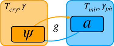
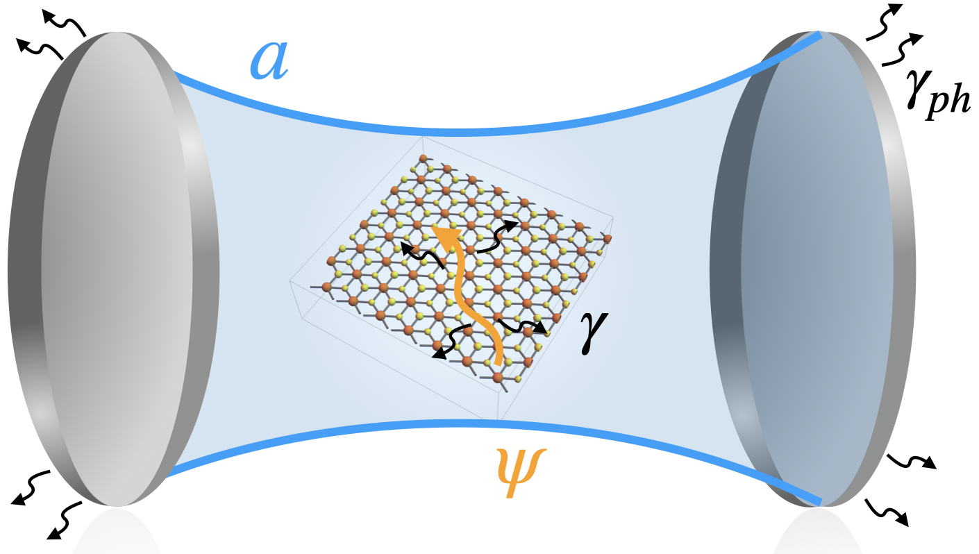
Figure 1: Schematic representation of the electron-photon system under consideration. a) Two distinct thermal baths coupled to the electrons (photons) $\Psi$ ($A$) and with temperature $T_{\rm cry}$ ($T_{\rm mir}$) and spectral width $\gamma$ ($\gamma_{\rm ph}$) in orange (blue). The electromagnetic potential $A$ is coupled to electrons with a strength $g$. b) Realization with a quantum material within a Fabry-Perot cavity.

The present work is particularly motivated by a recent experiment demonstrating cavity control of the metal-to-insulator transition in 1T-$\text{TaS}_{2}$ [24]. The critical temperature associated with the charge-density-wave formation could be substantially modified by tuning only the cavity resonant frequency [24], despite the light-matter coupling being small relative to the intrinsic electronic scales. So far, the cavity-induced Purcell effect has been suggested as a possible explanation [24, 25], whereby the electrons, due to the cavity environment, effectively experience a temperature different from the one of the cryostat.

In this work, we instead propose an alternative (or additional) mechanism: Despite the fact that an effective temperature can be extracted from the steady-state electronic distribution, we show that the leading-order effect on observables is genuinely non-thermal, as the standard Sommerfeld expansion is modified by a correction linearly proportional to the temperature difference, which cannot be predicted within the thermal Purcell effect. In this first work, we do not focus on the specific charge-density-wave scenario of [24], but rather consider a simpler model of a two-dimensional metal inside a Farby-Perot cavity, which makes the generic nature of the proposed non-thermal mechanism clear. We finally note that the non-thermal nature of the electronic distribution induced by cavity-photons has been already investigated in terms of its effect on the superconducting gap [19], in analogy to the original Eliashberg effect with oscillating radiofrequency fields [26]. Here we show that the cavity-induced non-thermal behaviour generically has a qualitative impact on any observable, since it breaks the symmetry of the theory [27] which forces the thermal Fermi-Dirac distribution to be anti-symmetric with respect to the Fermi surface.

Model.- We treat the cavity as two perfectly conducting parallel mirrors with the electrons moving in a plane parallel to the mirrors and placed amidst the latter, as schematically shown in Fig. 1(b). Photons inside the cavity acquire a finite mass because of the boundary conditions, which is set by the cavity fundamental frequency $\nu_{0}$, appearing in the photon dispersion $\nu(\textbf{q})^{2}=\nu_{0}^{2}+c^{2}\textbf{q}^{2}$. The Hamiltonian for the uncoupled, closed photon-electron system is given by:

$$H_{0}=\sum_{\textbf{k}}\epsilon(\textbf{k})\psi^{\dagger}_{\textbf{k}}\psi_{\textbf{k}}+\sum_{\textbf{q}}\nu(\textbf{q})\left(a^{\dagger}_{\textbf{q}}a_{\textbf{q}}+\dfrac{1}{2}\right),$$ (1)

where the first term models the metallic behaviour of the electrons with a gapless dispersion meaning $\epsilon(\textbf{k})=\lvert\textbf{k}\rvert^{2}/2m$ in $d+1$ space-time dimensions. We have expressed the Hamiltonian in terms of the creation and annihilation operators for the electrons $\{\psi_{\textbf{k}},\psi^{\dagger}_{\textbf{k}^{\prime}}\}=\delta_{\textbf{k},\textbf{k}^{\prime}}$ as well as for the cavity photons $[a_{\textbf{q}},a^{\dagger}_{\textbf{q}^{\prime}}]=\delta_{\textbf{q},\textbf{q}^{\prime}}$. We couple the electrons to a thermal bath at temperature $T_{\psi}$. Physically, this bath comes from the cryogenically cooled substrate. We choose the simplest model where the bath can be treated exactly. It is composed of fermionic degrees of freedom coupled linearly to the electrons:

$$H_{\text{e-bath}}=\sum_{\textbf{k},s}\epsilon_{s}(\textbf{k})f^{\dagger}_{s\textbf{k}}f_{s\textbf{k}}+t_{s}(\textbf{k})(\psi^{\dagger}_{\textbf{k}}f_{s\textbf{k}}+f^{\dagger}_{s\textbf{k}}\psi_{\textbf{k}}).$$ (2)

Here we have an extensive number of bath degrees of freedom $f_{s\textbf{k}}$, labeled by $s$ and coupled to each electron momentum component. As shown in the supplementary material, where we adopt a real-time-path-integral formulation on the Keldsyh contour [28, 29] to integrate the bath out, the latter enters the effective theory for the electrons via its temperature $T_{\psi}$ and the quasiparticle damping $\gamma(\textbf{k},\omega)$. A description in terms of these two quantities is actually more generally applicable than to the simple model of eq.(2). Additionally, cavity loss from the mirrors allows the external environmental photons to act as a thermal bath for the cavity modes. The Hamiltonian of the photon bath and coupling reads:

$$H_{\rm ph-bath}= \sum_{s,\textbf{q}}\nu_{s}(\textbf{q})\left(d^{\dagger}_{s\textbf{q}}d_{s\textbf{q}}+\dfrac{1}{2}\right)$$

$$+t^{\rm ph}_{s}(\textbf{q})(a^{\dagger}_{-\textbf{q}}+a_{\textbf{q}})(d^{\dagger}_{s-\textbf{q}}+d_{s\textbf{q}}),$$ (3)

where we again consider an extensive number of harmonic oscillators coupling to each photonic mode of the cavity in a linear fashion. As for the electrons, we integrate out the bath within our path-integral formulation to obtain an effective description in terms of the bath temperature $T_{\rm mir}$ and the resulting quasiparticle damping $\gamma_{\rm ph}(\mathbf{k},\omega)$. Finally, we model the electron-photon coupling as follows:

$$V=\dfrac{g}{\sqrt{N}}\sum_{\textbf{k},\textbf{q}}\psi^{\dagger}_{\textbf{k}+\textbf{q}}\psi_{\textbf{k}}(a^{\dagger}_{-\textbf{q}}+a_{\textbf{q}}),$$ (4)

where $g$ is the light-matter coupling. In Fabry-Perot cavities it is small, typically of the order of $0.1$ the electron bandwidth [30, 31, 32]. Note that we are using a coupling to the electron density and not the electron current. This might be appropriate for deep-subwavelength cavities [32], but for the Fabry-Perot cavity considered here, the current coupling should actually be used. Since it won’t modify our main message, for the sake of simplicity we consider a density coupling and also neglect its dependence on the photon momentum, such that a single coupling constant $g$ can be employed. The total Hamiltonian we consider is thus $H=H_{0}+H_{\rm e-bath}+H_{\rm ph-bath}+V$.

Dyson’s equation approach.— Our goal is to compute the electron distribution in the steady-state of the open system. We cannot assume thermal equilibrium, plus electrons and photons need in principle to be treated on equal footing. Therefore, a classical (Langevin or Fokker-Planck) approach is not suitable, while a standard Boltzmann-type equation for the electrons is restricted to the case of a small electron-bath coupling ensuring well-defined quasiparticles [19]. We thus choose to work with coupled Dyson’s equation for the electron’s and photon’s distribution functions. Since we are dealing with an interacting system – the electron-photon coupling is not linear – we adopt a self-consistent one-loop approach [33, 34] which can be obtained within the real-time-path-integral formulation illustrated in the Supplementary Material. Further assuming space- and time-translation invariance in the steady state, the resulting equation reads:

$$2\gamma(\omega)\Delta F(\textbf{k},\omega)=g^{2}\sum_{\textbf{k}^{\prime}}\int\differential\tilde{\omega}A(\textbf{k}^{\prime},\tilde{\omega})A_{ph}(\textbf{k}^{\prime}-\textbf{k},\tilde{\omega}-\omega)\times$$

$$(F(\textbf{k}^{\prime},\tilde{\omega})D_{0}(\tilde{\omega}-\omega)-1-F(\textbf{k},\omega)(D_{0}(\tilde{\omega}-\omega)-F(\textbf{k}^{\prime},\tilde{\omega})),$$ (5)

where we have defined $\Delta F(\textbf{k},\omega)=F(\textbf{k},\omega)-F_{0}(\omega)$, along with the thermal distribution functions for the electrons $F_{0}(\omega)=\tanh{(\omega-\mu_{0}))/(2T_{cry})}$ and the photons $D_{0}(\omega)=\coth(\omega/2T_{mir})$. We have also written the right hand side in terms of the spectral functions of the electrons $A(\textbf{k},\omega)$ and the photons $A_{\rm ph}(\textbf{k},\omega)$. The spectral functions are defined as $A(\textbf{k},\omega)=\dfrac{\gamma(\textbf{k},\omega)}{(\omega-\epsilon_{\textbf{k}})^{2}+\gamma^{2}(\textbf{k},\omega)},\ A_{\rm ph}(\textbf{q},\omega)=\dfrac{1}{L}\dfrac{\gamma_{\rm ph}(\omega)}{(\omega^{2}-\nu(\textbf{q})^{2})^{2}+\gamma_{\rm ph}^{2}(\omega)}$, where we introduced the cavity length $L$ which is inversely proportional to the fundamental frequency $\nu_{0}$. Within the simple model introduced above, the quasiparticle dampings are set by the baths spectral densities: $\gamma_{\rm ph}(\omega,\textbf{q})=\sum_{s}\frac{\pi t^{\rm ph}_{s}(\textbf{q})^{2}}{4\nu_{s}(\textbf{q})}\delta(\omega-\nu_{s}(\textbf{q}))$ for the photons and $\gamma(\omega,\textbf{k})=\frac{\pi}{2}\sum_{s}t_{s}^{2}(\textbf{k})\ \delta(\omega-\epsilon_{s}(\textbf{k}))$ for the electrons.

Equation (5) is obtained from the fully self-consistent approach by neglecting the back-action of the electrons onto the photons, which is valid as long as the photon-bath coupling, quantified by $\gamma_{\rm ph}$, is sufficiently larger than the coupling $g$. While the above equation is numerically solvable, we will show next that a fully analytical solution is also possible with a few further approximations which do not affect the main qualitative features. The first of this approximations is based on the assumption that the photon spectral function varies in frequency on a much smaller scale than the electron spectral function and the distribution function of both photons and electrons. In order for this to be true, the photon damping, setting the width of the spectral function, must be sufficiently smaller than the electron damping: $\gamma_{\rm ph}\ll\gamma$, as well as the temperatures: $\gamma_{\rm ph}\ll T_{\rm cry},T_{\rm mir}$ (as well shall see, the scale of variation in $F$ is actually always larger than $T_{\rm cry}$ due to the coupling to the hotter photon bath). Under these conditions, we can treat the photon spectral function as a Dirac-delta peaked at the photon dispersion to perform the frequency integral in eq.(5). Further, the momentum integral can be similarly performed by observing that the photons in the cavity have an extremely light mass since the speed of light is large, which allows to treat the momentum-dependence of the photon spectral function also as a Dirac-delta peaked at zero momentum.

[]
[]

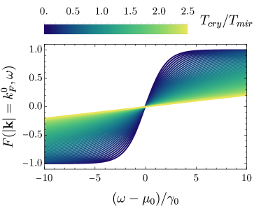
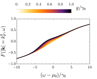
Figure 2: Distribution function for the solution of eq. (6). a) For different values of $T_{cry}\in(0,20)$ with fixed $T_{mir}=10$ and $g=0.2$ b) For different values of $g$ with fixed $T_{cry}=5$ and $T_{mir}=10$.

Finally, a fully analytical solution can be obtained in either one of two regimes: $\nu_{0}\ll T_{\rm mir}$ or $\nu_{0}\gg T_{\rm mir}$. In the Supplementary Material we show that the latter leads to the distribution function behaving just like the thermal $F_{0}(\omega)$ to lowest order. Instead, the opposite regime leads non-trivially to a non-linear differential equation for the distribution function of the form:

$$2T_{\rm mir} \dfrac{\partial F(\textbf{k},\omega)}{\partial\omega}=1-F(\textbf{k},\omega)^{2}+\dfrac{1}{2\tilde{A}_{0}}(F(\textbf{k},\omega)-F_{0}(\omega)),$$

$$\tilde{A}_{0}=\dfrac{\pi g^{2}S_{d-1}}{2L\nu_{0}}\dfrac{1}{(\omega-\epsilon_{\textbf{k}})^{2}+\gamma^{2}(\textbf{k},\omega)},$$ (6)

where we denoted $S_{d-1}$ as the volume of the $d-1$ sphere. We solve eq. (6) subject to the boundary condition of a filled Fermi sea $F(\omega)\rightarrow-1$ as $\omega\to-\infty$. The equation can be mapped to a Riccati equation and turned into a linear second order differential equation with non-constant coefficients, whose solution involves in general special functions.

Steady state distribution function.— The structure of equation (6) can be understood by looking at the physical limits where we know what must happen. For $g\rightarrow\infty$ the equation only retains the first two terms. With the boundary condition of a filled Fermi sea $F(\omega)\rightarrow-1$ as $\omega\to-\infty$, the solution is the Fermi-Dirac distribution with the photon-bath temperature $T_{\rm mir}$. This is natural since in this limit the coupling to the photons (and their respective bath) dominates. In the opposite limit $g\rightarrow 0$, the last term in eq.(5) is the only important one, such that the solution becomes $F=F_{0}$, which is trivially expected for a vanishing coupling to the photons.

For generic values of $g$ the electron distribution is instead non-thermal, and is shown in Fig. 2) for different values of the temperature ratio $T_{\rm cry}/T_{\rm mir}$ (see panel (a)), as well as of the light-matter coupling $g$ (see panel (b)). Note that in the regime considered, where the approximations listed above are valid, the solution does not depend anymore on the photon fundamental frequency $\nu_{0}$ and damping $\gamma_{\rm ph}$.The non-thermal nature of the distribution becomes clearly visible in Fig.2(b) by increasing $g$: the linear function $(\omega-\mu_{0})/T_{\rm cry}$ at $g=0$ is replaced by a function interpolating between two different slopes, one corresponding to a colder, one to a hotter temperature.

Broken thermal symmetry and Sommerfeld expansion.— In the remainder of this work however, we will concentrate on one particular non-thermal feature of the electron steady-state distribution and its effect on observables. This feature is illustrated in Fig.3 and compared with the thermal limits $g\to 0,\infty$. From the green dashed line it is clear that, while the thermal distribution is strictly anti-symmetric about the chemical potential as required by thermal equilibrium [27], the electron distribution in the generic case is not: $F(\omega-\mu)\neq F(-\omega+\mu)$. This can be also seen explicitly from the analytical form of the solution which can be obtained by linearizing the equation about, $\omega=\mu$. The solution involves the error function and is discussed in the supplementary material, a more illuminating expression can be obtained by expanding in powers of the small parameter $\tilde{g}=\sqrt{S_{d-1}}g/\gamma_{0}$, with $\gamma_{0}=\gamma(\epsilon_{\textbf{k}},\textbf{k})$, where the only momentum dependence is implicit and comes now through $\epsilon_{\textbf{k}}$, for the plots we specialize to the Fermi momentum $\lvert\textbf{k}_{F}^{0}\rvert=k_{F}^{0}$, defined as $k_{F}^{0}=\sqrt{2m\mu_{0}}$. Since we linearize we need for consistency also $\Delta T/T_{\rm cry}\ll 1$, where we have defined the temperature difference $\Delta T=T_{cry}-T_{mir}$. The leading order expression for the distribution then becomes:

$$F(\textbf{k},\omega)\approx F_{0}(\omega)+\dfrac{\Delta T}{T_{\rm cry}}\left(\dfrac{1}{\dfrac{\omega-\mu_{0}}{T_{\psi}}-\dfrac{1}{\tilde{g}^{2}}}\right),$$ (7)

From this expression we can clearly isolate the photon-induced modification of the electron thermal distribution $F_{0}$. We see that in the limit of small $\tilde{g}$ it is proportional to $\tilde{g}^{2}\Delta T/T_{\rm cry}$. It is proportional to the temperature difference between the two baths, as expected, thus $\Delta T$ also amplifies the photon-induced redistribution. The resulting $F$ has a shifted chemical potential defined by $F(\mu)=0$, given by $\mu=2\tilde{g}^{2}\Delta T+O(\tilde{g}^{6})$. Moreover, by linearizing about $\mu$ we can extract an effective temperature defined by $F\propto(\omega-\mu)/T_{\rm eff}$, with $T_{\rm eff}=T_{\rm cry}+(\tilde{g}^{2}(\Delta T)/T_{\rm cry})^{2}(1+T_{\rm cry}/\Delta T)$. In the same spirit of the thermal Purcell effect [24, 25], we can thus observe that the effective electron temperature starts depending on the temperature difference between the two baths.

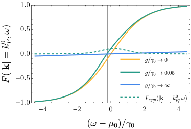
Figure 3: Distribution function for $T_{cry}=1,\ T_{mir}=50$ (solid lines). The dashed line corresponds to the symmetric component $F_{\text{ symm}}(k^{0}_{F},\omega)=F(k^{0}_{F},\omega-\mu)+F(k^{0}_{F},-\omega+\mu)$ with respect to $\mu$, the latter indicated with a black vertical line.

However, as well shall show next, the most important contribution to observables near the chemical potential comes from the non-thermal component of $F$, given by the non-antisymmetric part. In agreement with the dashed line of Fig.3, we see that $F$ indeed has also even powers in $\omega-\mu$, and these generate a non-thermal, leading order correction in a Sommerfeld expansion.

The simplest observables to characterize are single particle expectation values $\langle\hat{O}\rangle=\expectationvalue{\int dt\sum_{\textbf{k}}o_{\textbf{k}}(t)\psi_{\textbf{k}}(t)^{\dagger}\psi_{\textbf{k}}(t)}$. We can obtain a closed expression by assuming that the width $\gamma_{0}$ of the spectral function is much smaller than the region where the observable and occupation function vary appreciably, for simplicity we also take the quasiparticle damping to be a constant $\gamma(\epsilon_{\textbf{k}},\textbf{k})=\text{cte}=\gamma_{0}$. To leading order in $\tilde{g}$ this means: $T_{cry}\gg\gamma_{0}$. Under this approximation, and assuming that $o_{\textbf{k}}(0)=o_{\textbf{k}}(-\epsilon_{\textbf{k}})$, we recover the starting point for the usual Sommerfeld expansion (for details see the supplementary material): $\langle\hat{O}\rangle=\int\differential\epsilon\ O(\epsilon)\ D(\epsilon)(F(\epsilon)-1)/2$, where we defined the density of states $D(\epsilon)$. We can now generalize the Sommerfeld expansion for our non-thermal steady state using the approximated solution (7). The leading-order term quantifying the difference between the usual thermal expansion and the present case reads:

$$\Delta\langle\hat{O}\rangle \equiv\int\differential\epsilon\ O(\epsilon)\ D(\epsilon)(F(\epsilon)-F_{0}(\epsilon))/2$$ (8)

$$=(T_{\rm mir}-T_{\rm cry})\dfrac{S_{d-1}g^{2}}{\gamma_{0}^{2}}O(\mu)D(\mu)$$ (9)

We see that this new term is linear in the temperature difference and also proportional to the value of the observable at the chemical potential. Such a term is prohibited at thermal equilibrium due to the thermal symmetry excluding even terms of $F$ (see also supplementary material), such that the first temperature contribution is of higher order and contains the derivative of the observable: $(\pi^{2}T^{2}/6)\partial_{\epsilon}O(\epsilon)D(\epsilon)\lvert_{\mu}$.

Conclusions.— We have considered the non-thermal features of the electron distribution under the influence of two baths: one being the cryostat and the other the electromagnetic environment filtered by the presence of a Fabry-Perot cavity, as realized in state-of-the-art experimental setups. In particular, we have shown that the distribution breaks the thermal constraint of antisymmetry, resulting into a leading-order correction to the Sommerfeld expansion for observables around the Fermi surface. This finding might hint to a solution of the experimental puzzle recently presented in [24], and more generally shows that the influence of a small light-matter coupling is amplified through non-equilibrium effects.

Acknowledgements— We thank Mursalin Islam and Michele Pini for careful feedback on the derivations, as well as Martin Eckstein, Daniele Fausti, and Zala Lenarcic for fruitful discussions.

S1 Photon field coupled to a thermal bath

Starting with the general framework of a real photon field , which has $a$ as an annihilation operator,coupled to a bath we may model the bath as multiple real photon fields with different dispersions. The Keldish action for the photon field will be given generically by:

$$S_{\phi}= \sum_{\textbf{k}}\oint_{\mathcal{C}}Ldt\ \absolutevalue{\dot{\phi}(\textbf{k},t)}^{2}-\nu(\textbf{k})^{2}\absolutevalue{\phi(\textbf{k},t)}^{2}=\sum_{\textbf{k}}L\int_{-\infty}^{\infty}dt\ \absolutevalue{\dot{\phi}_{+}(\textbf{k},t)}^{2}-\nu(\textbf{k})^{2}\absolutevalue{\phi_{+}(\textbf{k},t)}^{2}-\absolutevalue{\dot{\phi}_{-}(\textbf{k},t)}^{2}+\nu(\textbf{k})^{2}\absolutevalue{\phi_{-}(\textbf{k},t)}^{2}$$ (S1)

$$=\sum_{\textbf{k}}\int_{-\infty}^{\infty}d\omega L\begin{pmatrix}\phi^{cl}(\textbf{k},\omega)^{*}&&\phi^{q}(\textbf{k},\omega)^{*}\end{pmatrix}\begin{pmatrix}0&&(\omega-i0)^{2}-\nu(\textbf{k})^{2}\\ (\omega+i0)^{2}-\nu(\textbf{k})^{2}&&2i0F(\omega)\end{pmatrix}\begin{pmatrix}\phi^{cl}(\textbf{k},\omega)\\ \phi^{q}(\textbf{k},\omega)\end{pmatrix},$$ (S2)

where the first line describes the field along the Keldysh contour being expressed in terms of the $+,-$ branches. We have also introduced a length which has units of inverse energy and in cavities comes from the $z$ axis boundary conditions that quantize the energy, this also has the added benefit of giving the field $\phi(x,t)$ dimensionless units. The second line is fourier transformed for each branch and a Keldysh rotation has been applied meaning $\phi^{cl,q}=(\phi_{+}\pm\phi_{-})/2$ and the infinitesimal $\pm i0$ are needed to express the physical coupling of the two branches at $t=-\infty$ given by the initial density matrix. $F(\omega)$ is likewise a distribution function for the correct normalization which will be replaced by the finite coupling to the bath. The bath will have the same structure but for multiple frequencies meaning an action of the form:

$$S_{\theta}=\sum_{\textbf{k},s}\int_{-\infty}^{\infty}d\omega L\begin{pmatrix}\theta_{s}^{cl}(\textbf{k},\omega)^{*}&&\theta_{s}^{q}(\textbf{k},\omega)^{*}\end{pmatrix}\begin{pmatrix}0&&(\omega-i0)^{2}-\nu_{s}(\textbf{k})^{2}\\ (\omega+i0)^{2}-\nu_{s}(\textbf{k})^{2}&&2i0D(\omega)\end{pmatrix}\begin{pmatrix}\theta_{s}^{cl}(\textbf{k},\omega)\\ \theta_{s}^{q}(\textbf{k},\omega)\end{pmatrix},$$ (S3)

where $\theta_{s}^{q}(\textbf{k},\omega)$ are now the bath variables and $D_{0}(\omega)=\coth(\omega/2T_{mir})$ is the distribution function assuming the bath is in thermal equilibrium, which not necessarily implies the $\phi$ field is. To model the coupling between the bath and field we take the simple interaction:

$$S_{\theta\phi}=\sum_{\textbf{k},s}\oint_{\mathcal{C}}dt\ Lt_{s}^{ph}\phi(\textbf{k},t)\theta_{s}(\textbf{k},t)=\sum_{\textbf{k},s}\int_{-\infty}^{\infty}Ld\omega\ t_{s}^{ph}\Phi(\textbf{k},\omega)^{\dagger}\tau_{x}\Theta_{s}(\textbf{k},\omega),$$ (S4)

where the coupling changes for each field and is dimensionless by virtue of the the $L$ factor the final vector fields are in Keldysh space meaning $\Phi(\textbf{k},\omega)^{T}=\begin{pmatrix}\phi^{cl}(\textbf{k},\omega)&&\phi^{q}(\textbf{k},\omega)\end{pmatrix}$ and $\Theta_{s}(\textbf{k},\omega)=\begin{pmatrix}\theta_{s}^{cl}(\textbf{k},\omega)&&\theta_{s}^{q}(\textbf{k},\omega)\end{pmatrix}$. The matrix $\tau_{x}$ is just the first Pauli matrix in the Keldysh space. Now if one wants to obtain properties of the stationary state but arbitrary long time correlations then the Keldysh partition function is expressed as:

$$Z_{\phi}=\dfrac{\Tr{\rho(t_{f}\rightarrow\infty)}}{\Tr{\rho(t_{i}\rightarrow-\infty)}}=\int\mathcal{D}(\phi^{cl},\phi^{q})\prod_{s}\mathcal{D}(\theta_{s}^{cl},\theta_{s}^{q})\ e^{iS[\phi,\theta_{s}]}=\int\mathcal{D}(\phi^{cl},\phi^{q})\ e^{iS_{\phi}[\phi]}\int\prod_{s}\mathcal{D}(\theta_{s}^{cl},\theta_{s}^{q})\ e^{i(S_{\theta}+S_{\phi\theta})},$$ (S5)

where the trace of the initial density matrix is taken into account in the normalization. Due to the action being quadratic it is possible to integrate out the $\theta_{s}$ fields and get an effective action for the $\phi$ photon field. In this case we must perform a Gaussian integral which results on the inverse of the matrix in eq. S3 and matrices coming from the coupling which has a $\tau_{x}$ Pauli Matrix. This means we can define:

$$\tilde{D}(\textbf{k},\omega)=-\tau_{x}\sum_{s}(t_{s}^{ph})^{2}D_{s}(\textbf{k},\omega)\tau_{x},\qquad D_{s}(\textbf{k},\omega)=\begin{pmatrix}D_{s}^{K}(\textbf{k},\omega)&&D_{s}^{R}(\textbf{k},\omega)\\ D_{s}^{A}(\textbf{k},\omega)&&0\end{pmatrix},\qquad\tilde{D}(\textbf{k},\omega)=\begin{pmatrix}0&&\tilde{D}^{A}(\textbf{k},\omega)\\ \tilde{D}^{R}(\textbf{k},\omega)&&\tilde{D}^{K}(\textbf{k},\omega)\end{pmatrix}$$ (S6)

where the previous matrix in the action is defined as the inverse of the propagator $D$ meaning that we have also the following relations:

$$D_{s}^{(R,A)}(\textbf{k},\omega)=\dfrac{1}{2L}\dfrac{1}{(\omega\pm i0)^{2}-\nu_{s}^{2}(\textbf{k})},\qquad D^{K}_{s}(\textbf{k},\omega)=\coth{\frac{\omega}{2T_{mir}}}(D^{R}_{s}(\textbf{k},\omega)-D^{A}_{s}(\textbf{k},\omega)),$$ (S7)

where we have assumed that the bath is in thermal equilibrium so that the fluctuation-dissipation theorem relates the Keldysh Green’s function to the retarder and advanced Green’s functions. Focusing on the retarded and advanced Green’s functions we obtain:

$$\tilde{D}^{(R,A)}(\textbf{k},\omega)=-\frac{1}{2L}\sum_{s}\dfrac{(t_{s}^{ph})^{2}L^{2}}{(\omega\pm i0)^{2}-\nu_{s}^{2}(\textbf{k})}=L\int\dfrac{d\tilde{\omega}}{2\pi}\dfrac{\tilde{\omega}J(\textbf{k},\tilde{\omega})}{\tilde{\omega}^{2}-(\omega\pm i0)^{2}}\qquad J(\textbf{k},\omega)=\pi\sum_{s}\dfrac{(t_{s}^{ph})^{2}}{\nu_{s}(\textbf{k})}\delta(\omega-\nu_{s}(\textbf{k})),$$ (S8)

where we defined the bath spectral density as $J(\textbf{k},\omega)$ generically one can think of the spectral density of the bath as being some function of the frequency which is continuous in the real axis and decays faster than $1/\omega$ if thought as a complex function. In this case we can apply the Sokhotski–Plemelj theorem which states for real functions that :

$$\lim_{\varepsilon\rightarrow 0^{+}}\int_{a}^{b}\frac{f(x)}{x\pm i\varepsilon}dx=\mp i\pi f(0)+\mathcal{P}\int_{a}^{b}\frac{f(x)}{x}dx.$$ (S9)

In this case we can use it for $x=\tilde{\omega}^{2}-\omega^{2}$ and $\pm i\epsilon$ will be $\mp 2i0\omega$ so that one obtains :

$$\tilde{D}^{(R,A)}(\textbf{k},\omega)=L\mathcal{P}\int\dfrac{dx}{2\pi}\dfrac{J(\textbf{k},x)}{x}\pm i2L\gamma_{ph}(\textbf{k},\omega)=cte.\pm i2L\gamma_{ph}(\textbf{k},\omega),$$ (S10)

where we have defined $J$ so that one obtains also for the Keldysh Green’s function the result:

$$\tilde{D}^{K}(\textbf{k},\omega)=4i\gamma_{ph}(\textbf{k},\omega)LD_{0}(\omega),\quad\gamma_{ph}(\textbf{k},\omega)=J(\textbf{k},\omega)/4.$$ (S11)

In this way integrating out the bath variables leads to a contribution to the photon field action of the form:

$$\frac{1}{2}\sum_{\textbf{k}}\int_{-\infty}^{\infty}d\omega\Phi(\textbf{k},\omega)^{\dagger}\tilde{D}(\textbf{k},\omega)\Phi(\textbf{k},\omega).$$ (S12)

The combined integration thus leads to an effective action which now has a finite Keldysh component as well as imaginary parts in the retarded and advanced Green’s functions giving rise to the partition function of the form:

$$Z =\int\mathcal{D}(\phi^{cl},\phi^{q})\exp{i\sum_{\textbf{k}}\int_{-\infty}^{\infty}d\omega L\Phi^{\dagger}\begin{pmatrix}0&&\omega^{2}-\nu(\textbf{k})^{2}-i\gamma_{ph}(\textbf{k},\omega)\\ \omega^{2}-\nu(\textbf{k})^{2}+i\gamma_{ph}(\textbf{k},\omega)&&2i\gamma_{ph}(\textbf{k},\omega)D_{0}(\omega)\end{pmatrix}\Phi},$$ (S13)

where the constant change in the retarded and advanced functions was absorbed in the dispersion relation of the photon field.

S2 Electron field coupled to thermal bath

Analogously to the previous section we can consider the electrons coupled to a bath which physically could be the phonons of a lattice system. Since we consider only the generic change in behaviour to a thermal bath the may as well couple the electrons to another fermion system which will allow for analytically exact results in comparison to the phonon case but the overall generic behaviour. To test this we consider a fermion field with the corresponding action:

$$S_{\psi}= \sum_{\textbf{k}}\oint_{\mathcal{C}}dt\ \bar{\psi}(\textbf{k},t)(i\partial_{t}-\epsilon(\textbf{k}))\psi(\textbf{k},t)=\sum_{\textbf{k}}\int_{-\infty}^{\infty}dt\ \bar{\psi}_{+}(\textbf{k},t)(i\partial_{t}-\epsilon(\textbf{k}))\psi_{+}(\textbf{k},t)-\bar{\psi}_{-}(\textbf{k},t)(i\partial_{t}-\epsilon(\textbf{k}))\psi_{-}(\textbf{k},t)$$ (S14)

$$=\sum_{\textbf{k}}\int_{-\infty}^{\infty}d\omega\begin{pmatrix}\bar{\psi}^{cl}(\textbf{k},\omega)&&\bar{\psi}^{q}(\textbf{k},\omega)\end{pmatrix}\begin{pmatrix}\omega-\epsilon(\textbf{k})+i0&&2i0P(\omega)\\ 0&&\omega-\epsilon(\textbf{k})-i0\end{pmatrix}\begin{pmatrix}\psi^{cl}(\textbf{k},\omega)\\ \psi^{q}(\textbf{k},\omega)\end{pmatrix},$$ (S15)

where the first line describes the field along the Keldysh contour being expressed in terms of the $+,-$ branches and the second line is Fourier transformed for each branch and a Keldysh rotation has been applied. For Fermions the Keldysh rotation is defined as $\psi^{(cl,q)}=(\psi_{+}\pm\psi_{-})/\sqrt{2}$ and by convention $\bar{\psi}^{(cl,q)}=(\bar{\psi}_{+}\mp\bar{\psi}_{-})/\sqrt{2}$. We can now think similarly to the previous case on a fermionic bath which is coupled to the previous electron field with the action:

$$S_{\upsilon} =\sum_{\textbf{k},s}\int_{-\infty}^{\infty}d\omega\begin{pmatrix}\bar{\upsilon}_{s}^{cl}(\textbf{k},\omega)&&\bar{\upsilon}_{s}^{q}(\textbf{k},\omega)\end{pmatrix}\begin{pmatrix}\omega-\epsilon_{s}(\textbf{k})+i0&&2i0F_{0}(\omega)\\ 0&&\omega-\epsilon_{s}(\textbf{k})-i0\end{pmatrix}\begin{pmatrix}\upsilon_{s}^{cl}(\textbf{k},\omega)\\ \upsilon_{s}^{q}(\textbf{k},\omega)\end{pmatrix},$$ (S16)

where $\upsilon_{s}^{q}(\textbf{k},\omega)$ are now the bath variables and $F_{0}(\omega)=\tanh((\omega-\mu_{0})/2T_{cry})$ is the distribution function assuming the bath is in thermal equilibrium, which not necessarily implies the $\psi$ field is. To model the coupling between the bath and field we take the simplest interaction:

$$S_{\psi\upsilon}=\sum_{\textbf{k},s}t_{s}\oint_{\mathcal{C}}dt\ \bar{\psi}(\textbf{k},t)\upsilon_{s}(\textbf{k},t)+\bar{\upsilon}_{s}(\textbf{k},t)\psi(\textbf{k},t)=\sum_{\textbf{k},s}t_{s}\int_{-\infty}^{\infty}d\omega\ \bar{\Psi}(\textbf{k},\omega)^{T}\gamma^{cl}\Upsilon_{s}(\textbf{k},\omega)+\bar{\Upsilon}_{s}(\textbf{k},\omega)^{T}\gamma^{cl}\Psi(\textbf{k},\omega),$$ (S17)

where the coupling changes for each field and the final vector fields are in Keldysh space meaning $\bar{\Psi}(\textbf{k},\omega)^{T}=\begin{pmatrix}\bar{\psi}^{cl}(\textbf{k},\omega)&&\bar{\psi}^{q}(\textbf{k},\omega)\end{pmatrix}$ and $\Upsilon_{s}(\textbf{k},\omega)=\begin{pmatrix}\eta_{s}^{cl}(\textbf{k},\omega)&&\eta_{s}^{q}(\textbf{k},\omega)\end{pmatrix}$. The matrix $\gamma^{cl}=\hat{1}$ is just the zeroth Pauli matrix in the Keldysh space. Now if one wants to obtain properties of the stationary state but arbitrary long time correlations then the Keldysh partition function is expressed as:

$$Z_{\psi}=\dfrac{\Tr{\rho(t_{f}\rightarrow\infty)}}{\Tr{\rho(t_{i}\rightarrow-\infty)}}=\int\mathcal{D}(\bar{\Psi},\Psi)\prod_{s}\mathcal{D}(\bar{\Upsilon}_{s},\Upsilon_{s})\ e^{iS[\Psi,\Upsilon_{s}]}=\int\mathcal{D}(\bar{\Psi},\Psi)\ e^{iS_{\psi}}\prod_{s}\mathcal{D}(\bar{\Upsilon}_{s},\Upsilon_{s})\ e^{i(S_{\upsilon}+S_{\psi\upsilon})},$$ (S18)

now since the action for the bath is again quadratic we can integrate them exactly to obtain an effective contribution to the $\psi$ field. In this case the integral of Grassman variables changes the form of the resulting integral so that it is useful to define:

$$\tilde{P}(\textbf{k},\omega)=-\sum_{s}t_{s}^{2}P_{s}(\textbf{k},\omega),\qquad P_{s}(\textbf{k},\omega)=\begin{pmatrix}P_{s}^{R}(\textbf{k},\omega)&&P_{s}^{K}(\textbf{k},\omega)\\ 0&&P_{s}^{A}(\textbf{k},\omega)\end{pmatrix},$$ (S19)

where the previous matrix in the action is defined as the inverse of the propagator $P$ meaning that we have also the following relations:

$$P_{s}^{(R,A)}(\textbf{k},\omega)=\dfrac{1}{\omega-\epsilon_{s}(\textbf{k})\pm i0},\qquad P^{K}_{s}(\textbf{k},\omega)=\tanh(\dfrac{\omega-\mu_{0}}{2T_{cry}})(P^{R}_{s}(\textbf{k},\omega)-P^{A}_{s}(\textbf{k},\omega)),$$ (S20)

where we have assumed that the bath is in thermal equilibrium so that the fluctuation-dissipation theorem applies. Focusing on the retarded and advanced Green’s functions we obtain:

$$\tilde{P}^{(R,A)}(\textbf{k},\omega)=-\sum_{s}\dfrac{t_{s}^{2}}{\omega-\epsilon_{s}(\textbf{k})\pm i0}=\int\dfrac{d\tilde{\omega}}{2\pi}\dfrac{\rho(\textbf{k},\tilde{\omega})}{\tilde{\omega}-\omega\mp i0}\qquad\rho(\textbf{k},\omega)=2\pi\sum_{s}t_{s}^{2}\ \delta(\omega-\epsilon_{s}(\textbf{k})).$$ (S21)

Applying again the Sokhotsky-Plemelj theorem with $x=\tilde{\omega}-\omega$ one obtains the result for the Greens function:

$$\tilde{P}^{(R,A)}(\textbf{k},\omega)=\mathcal{P}\int\dfrac{dx}{2\pi}\dfrac{\rho(\textbf{k},x)}{x}\pm i2\gamma(\textbf{k},\omega)=cte.\pm i2\gamma(\textbf{k},\omega),$$ (S22)

where we have defined $\gamma$ so that one obtains also for the Keldysh Green’s function the result:

$$\tilde{P}^{K}(\textbf{k},\omega)=4i\gamma(\textbf{k},\omega)F_{0}(\omega),\quad\gamma(\textbf{k},\omega)=\rho(\textbf{k},\omega)/4.$$ (S23)

In this way integrating out the bath variables leads to a contribution to the electronic field action of the form:

$$\sum_{\textbf{k}}\int_{-\infty}^{\infty}d\omega\bar{\Psi}(\textbf{k},\omega)^{T}\tilde{P}(\textbf{k},\omega)\Psi(\textbf{k},\omega).$$ (S24)

The combined integration thus leads to an effective action which now has a finite keldysh component as well as imaginary parts in the retarded and advanced Green’s functions giving rise to the partition function of the form:

$$Z =\int\mathcal{D}(\bar{\Psi},\Psi)\ e^{iS_{eff}[\psi]} =\int\mathcal{D}(\bar{\Psi},\Psi)\exp{i\sum_{\textbf{k}}\int_{-\infty}^{\infty}d\omega\bar{\Psi}^{T}\begin{pmatrix}\omega-\epsilon(\textbf{k})+i\gamma(\textbf{k},\omega)&&2i\gamma(\textbf{k},\omega)F_{0}(\omega)\\ 0&&\omega-\epsilon(\textbf{k})-i\gamma(\textbf{k},\omega)\end{pmatrix}\Psi},$$ (S25)

where the constant change in the retarded and advanced functions was absorbed in the dispersion relation of the photon field.

S3 Photon-Electron system and Dyson’s equation

We are now interested in what happens to the two bath configuration in general when we add a coupling between the electrons and the photons, specifically specializing in the steady state resulting from such interactions. To address this we introduce a a Yukawa type interaction:

$$S_{int} =g\oint_{\mathcal{C}}\differential t\int\differential^{d}\bm{x}\ \phi(\bm{x},t)\bar{\psi}(\bm{x},t)\psi(\bm{x},t)=g\int_{-\infty}^{\infty}\differential t\int\differential^{d}\bm{x}\ \phi_{+}(\bm{x},t)\bar{\psi}_{+}(\bm{x},t)\psi_{+}(\bm{x},t)-\phi_{-}(\bm{x},t)\bar{\psi}_{-}(\bm{x},t)\psi_{-}(\bm{x},t)$$ (S26)

$$=g\int_{-\infty}^{\infty}\differential t\int\differential^{d}\bm{x}\ \ \Phi_{\alpha}(\bm{x},t)\bar{\Psi}_{a}(\bm{x},t)\gamma^{\alpha}_{ab}\Psi_{b}(\bm{x},t),\qquad\gamma^{cl}=\begin{pmatrix}1&&0\\ 0&&1\end{pmatrix},\quad\gamma^{q}=\begin{pmatrix}0&&1\\ 1&&0\end{pmatrix}.$$ (S27)

A good check is to see what the units of the coupling are by using the fact that previously all fields in time had dimensionless units which means for the interacting part of the action to be dimensionless we must require $g$ to have units of energy. In cavities the coupling has indeed units of energy and is typically of the order $0.1t$ for a hopping parameter $t$ of the electrons. If one is interested in the form of the Green’s function for long times meaning analyzing properties of the steady state one will generally accumulate errors in time if one uses a perturbative approach. It is in this spirit that non-perturbative approaches such as the self-consistent formulation in terms of the effective action lead to information not being lost specifically conserved quantities. It is in this spirit that one defines a quantity $\Gamma$ which is gauge invariant and respects the microscopic symmetries from which one can obtain the self-energy of the system. To derive the corresponding equations is useful to define the following Feynman diagrams:

$$\fmffile{1}iG_{ab}(x,x^{\prime})=\hskip 28.45274pt\begin{gathered}\fmfgraph*(60,40)\fmfstraight\fmfleft{i1}\fmfright{o1}\fmf{dbl_{p}lain_{a}rrow}{i1,o1}\fmflabel{$b,x'$}{i1}\fmflabel{$a,x$}{o1}\end{gathered}\hskip 28.45274pt=\int\mathcal{D}(\bar{\Psi},\Psi)\int\mathcal{D}\Phi\ e^{iS[\Psi,\Phi]}\Psi_{a}(x)\bar{\Psi}_{b}(x^{\prime})=\expectationvalue{\Psi_{a}(x)\bar{\Psi}_{b}(x^{\prime})}$$ (S28)

$$\fmffile{2}iG^{0}_{ab}(x,x^{\prime})=\hskip 28.45274pt\begin{gathered}\fmfgraph*(60,40)\fmfstraight\fmfleft{i1}\fmfright{o1}\fmf{fermion}{i1,o1}\fmflabel{$b,x'$}{i1}\fmflabel{$a,x$}{o1}\end{gathered}\hskip 28.45274pt=\expectationvalue{\Psi_{a}(x)\bar{\Psi}_{b}(x^{\prime})}_{0}$$ (S30)

$$\fmffile{3}iU_{\alpha\beta}(x,x^{\prime})=\hskip 28.45274pt\begin{gathered}\fmfgraph*(60,40)\fmfstraight\fmfleft{i1}\fmfright{o1}\fmf{dbl_{w}iggly}{i1,o1}\fmflabel{$\beta,x'$}{i1}\fmflabel{$\alpha,x$}{o1}\end{gathered}\hskip 28.45274pt=\int\mathcal{D}(\bar{\Psi},\Psi)\int\mathcal{D}\Phi\ e^{iS[\Psi,\Phi]}\Phi_{\alpha}(x)\Phi_{\beta}(x^{\prime})=\expectationvalue{\Phi_{\alpha}(x)\Phi_{\beta}(x^{\prime})}$$ (S32)

$$\fmffile{4}iU^{0}_{\alpha\beta}(x,x^{\prime})=\hskip 28.45274pt\begin{gathered}\fmfgraph*(60,40)\fmfstraight\fmfleft{i1}\fmfright{o1}\fmf{boson}{i1,o1}\fmflabel{$\beta,x'$}{i1}\fmflabel{$\alpha,x$}{o1}\end{gathered}\hskip 28.45274pt=\expectationvalue{\Phi_{\alpha}(x)\Phi_{\beta}(x^{\prime})}_{0}$$ (S34)

$$\hskip 85.35826pt\fmffile{5}\begin{gathered}\fmfgraph*(60,40)\fmfleft{i1,o1}\fmfright{o2}\fmf{plain}{i1,v1,o1}\fmf{boson}{v1,o2}\fmflabel{$b$}{i1}\fmflabel{$a$}{o1}\fmflabel{$\alpha$}{o2}\fmflabel{$x$}{v1}\end{gathered}\hskip 28.45274pt=ig\gamma^{\alpha}_{ab}$$

where the expectation values in the path integral language are already path ordered in the operator language over the Keldysh contour and the last diagram represents the interaction vertex where the plain straight lines are the end and beginning of the propagators only. In the conserving approximation one defines an effective action in terms of bubble diagrams which have no external legs and defines the self-energy to be the functional derivative with respect to the propagators:

$$\Sigma^{\psi}_{ab}(x,x^{\prime})=\dfrac{\delta\Gamma}{\delta G_{ba}(x^{\prime},x)}\qquad\Sigma^{\phi}_{\alpha\beta}(x,x^{\prime})=\dfrac{\delta\Gamma}{\delta U_{\beta\alpha}(x^{\prime},x)}.$$ (S36)

The previous relation holds up to a combinatorial factor that counts the number of equivalent diagrams(the factor is $1/n$ for $n$ vertices) and a $\pm$ sign for photons or electrons.We can now define the effective action in terms of the fully dressed propagators to first order in the photon propagator:

$$\fmffile{a1}\Gamma^{HF}=\hskip 28.45274pt\begin{gathered}\fmfgraph(120,80)\fmfleft{v1}\fmfright{v4}\fmf{dbl_{p}lain_{a}rrow,left}{v1,v2}\fmf{dbl_{p}lain_{a}rrow,left}{v2,v1}\fmf{boson}{v2,v3}\fmf{dbl_{p}lain_{a}rrow,left}{v3,v4}\fmf{dbl_{p}lain_{a}rrow,left}{v4,v3}\end{gathered}\hskip 14.22636pt+\hskip 14.22636pt\fmffile{a2}\begin{gathered}\fmfgraph(50,30)\fmfleft{v1}\fmfright{v2}\fmf{dbl_{w}iggly}{v1,v2}\fmffreeze\fmf{dbl_{p}lain_{a}rrow,left}{v1,v2}\fmf{dbl_{p}lain_{a}rrow,left}{v2,v1}\end{gathered}\hskip 14.22636pt+\hskip 14.22636pt\dots$$ (S39)

In this approximation we obtain that the self-energy is given by:

$$\Sigma^{\psi}_{ab}(x,x^{\prime})=-ig^{2}\delta(x-x^{\prime})\int\differential y\ \gamma^{\alpha}_{ab}\gamma^{\alpha^{\prime}}_{a^{\prime}b^{\prime}}U_{\alpha\alpha^{\prime}}^{0}(x,y)G_{b^{\prime}a^{\prime}}(y,y)+ig^{2}\gamma^{\alpha}_{ab^{\prime}}\gamma^{\alpha^{\prime}}_{a^{\prime}b}U_{\alpha\alpha^{\prime}}(x,x^{\prime})G_{b^{\prime}a^{\prime}}(x,x^{\prime}),$$ (S40)

while for the photon to lowest order the first term (Hartree) doesn’t contribute since it has no dressed propagator and the second one gives the bubble diagram self energy:

$$\Sigma^{\phi}_{ab}(x,x^{\prime})=-ig^{2}\gamma^{\alpha}_{ab}\gamma^{\beta}_{b^{\prime}a^{\prime}}G_{bb^{\prime}}(x,x^{\prime})G_{a^{\prime}a}(x^{\prime},x).$$ (S41)

We can make use of the self-energy to obtain steady-state behaviour by substituting and solving self-consistently in the Dyson equation:

$$\fmffile{Dyson1}\begin{gathered}\fmfgraph*(60,40)\fmfstraight\fmfleft{i1}\fmfright{o1}\fmf{dbl_{p}lain_{a}rrow}{i1,o1}\end{gathered}\hskip 14.22636pt=\hskip 14.22636pt\fmffile{Dyson2}\begin{gathered}\fmfgraph*(60,40)\fmfstraight\fmfleft{i1}\fmfright{o1}\fmf{fermion}{i1,o1}\end{gathered}\hskip 14.22636pt+\hskip 14.22636pt\fmffile{Dyson3}\begin{gathered}\Large\color[rgb]{1,1,1}\fmfgraph*(100,40)\fmfstraight\fmfleft{i1}\fmfright{o1}\fmfblob{1cm}{v1}\fmf{fermion}{i1,v1}\fmf{dbl_{p}lain_{a}rrow}{v1,o1}\end{gathered},$$ (S44)

where the shaded circle represents the self-energy $\Sigma$. When written in terms of the Keldysh components it becomes:

$$((G_{0}^{R/A})^{-1}-\Sigma^{R/A}_{\psi})\circ G^{R/A}=\delta(x-x^{\prime}),\qquad G^{K}=G^{R}\circ(-(G_{0}^{K})^{-1}+\Sigma^{K}_{\psi})\circ G^{A}$$ (S45)

$$((U_{0}^{R/A})^{-1}-\Sigma^{R/A}_{\phi})\circ U^{R/A}=\delta(x-x^{\prime}),\qquad U^{K}=G^{R}\circ(-(U_{0}^{K})^{-1}+\Sigma^{K}_{\phi})\circ U^{A}.$$ (S46)

Now it is common to reparameterize the anti-hermitian Keldysh Green’s function in terms of a hermitian function $F$ defined by $G^{K}=G^{R}\circ F-F\circ G^{A}$. Using the previous Dyson equations one obtains:

$$(G_{0}^{K})^{-1} =G_{R}^{-1}\circ F-F\circ G_{A}^{-1}+\Sigma^{K}$$ (S47)

$$=((G_{0}^{R})^{-1}-\Sigma^{R})\circ F-F\circ((G_{0}^{A})^{-1}-\Sigma^{A}))+\Sigma^{K}$$ (S48)

$$=\Sigma^{K}-(\Sigma^{R}\circ F-F\circ\Sigma^{A})+((G_{0}^{R})^{-1}\circ F-F\circ(G_{0}^{A})^{-1}).$$ (S49)

Assuming stationarity or time translation invariance and space translation invariance while using the identities $(G^{R})^{\dagger}=G^{A}$, $(G^{K})^{\dagger}=-G^{K}$ we can obtain the quantum kinetic equations (QKE):

$$2i\gamma(\textbf{k},\omega)(F_{0}(\omega)-F(\textbf{k},\omega))=\Sigma^{K}_{\psi}(\textbf{k},\omega)-2iF(\textbf{k},\omega)\imaginary\Sigma^{R}_{\psi}(\textbf{k},\omega)$$ (S50)

$$2i\gamma_{ph}(\textbf{k},\omega)(D_{0}(\omega)-D(\textbf{k},\omega))=\Sigma^{K}_{\phi}(\textbf{k},\omega)-2iD(\textbf{k},\omega)\imaginary\Sigma_{\phi}^{R}(\textbf{k},\omega),$$ (S51)

where we used the previously derived non-interacting Green’s function obtained from integrating out the bath degrees of freedom. Since the bath gave a generic tunable function $F_{0}$ this will not generically equal the thermal $F_{th}$ which means the right side of the QKE is not zero meaning the steady state can be non-thermal. Written explicitly the Keldysh and retarded self-energies of the electrons one obtains:

$$\Sigma^{K}_{\psi}(x,x^{\prime})=ig^{2}(G^{K}(x,x^{\prime})U^{K}(x^{\prime},x)-(G^{R}(x,x^{\prime})-G^{A}(x,x^{\prime}))(U^{R}(x^{\prime},x)-U^{A}(x^{\prime},x)))$$ (S52)

$$\Sigma^{R}_{\psi}(x,x^{\prime})=-ig^{2}\delta(x-x^{\prime})\int\differential yU_{0}^{R}(x,y)G^{K}(y,y)+ig^{2}(G^{R}(x,x^{\prime})U^{K}(x^{\prime},x)+G^{K}(x,x^{\prime})U^{A}(x^{\prime},x)),$$ (S53)

where we used the causality identities $G^{R}(x,y)U^{R}(y,x)=0,\ G^{R}(x,x)+G^{A}(x,x)=0$ and others similar. We now take as a first approximation that the coupling $g$ between photons and electrons is very small compared to the dissipative terms of the baths $\gamma,\gamma_{ph}$ and the photon cavity frequency $\nu_{0}$ so that we can use the retarded and advanced functions of the non-interacting limit. So that $U^{K}_{0}(\textbf{k},\omega)=D_{0}(\omega)(U^{R}_{0}(\textbf{k},\omega)-U^{A}_{0}(\textbf{k},\omega))$ is satisfied and we can obtain:

$$\Sigma^{K}_{\psi}(\textbf{k},\omega)=ig^{2}\int\differential^{d}\textbf{k}^{\prime}\int\differential\tilde{\omega}(G^{R}(\textbf{k}^{\prime},\tilde{\omega})-G^{A}(\textbf{k}^{\prime},\tilde{\omega}))(U^{R}(\textbf{k}^{\prime}-\textbf{k},\tilde{\omega}-\omega)-U^{A}(\textbf{k}^{\prime}-\textbf{k},\tilde{\omega}-\omega))(F(\textbf{k}^{\prime},\tilde{\omega})D_{0}(\tilde{\omega}-\omega)-1)$$ (S54)

$$\Sigma^{R}_{\psi}(\textbf{k},\omega)-\Sigma^{A}_{\psi}(\textbf{k},\omega)=ig^{2}\int\differential^{d}\textbf{k}^{\prime}\int\differential\tilde{\omega}(G^{R}(\textbf{k}^{\prime},\tilde{\omega})-G^{A}(\textbf{k}^{\prime},\tilde{\omega}))(U^{R}(\textbf{k}^{\prime}-\textbf{k},\tilde{\omega}-\omega)-U^{A}(\textbf{k}^{\prime}-\textbf{k},\tilde{\omega}-\omega))$$

$$\hskip 312.9803pt\times(D_{0}(\tilde{\omega}-\omega)-F(\textbf{k}^{\prime},\tilde{\omega})),$$ (S55)

the corresponding QKE for the electrons becomes:

$$2i\gamma(\textbf{k},\omega)(F_{0}(\omega)-F(\textbf{k},\omega))=ig^{2}\int\differential^{d}\textbf{k}^{\prime}\int\differential\tilde{\omega}(G^{R}_{0}(\textbf{k}^{\prime},\tilde{\omega})-G^{A}_{0}(\textbf{k}^{\prime},\tilde{\omega}))(U^{R}_{0}(\textbf{k}^{\prime}-\textbf{k},\tilde{\omega}-\omega)-U^{A}_{0}(\textbf{k}^{\prime}-\textbf{k},\tilde{\omega}-\omega))$$

$$(F(\textbf{k}^{\prime},\tilde{\omega})D_{0}(\tilde{\omega}-\omega)-1-F(\textbf{k},\omega)(D_{0}(\tilde{\omega}-\omega)-F(\textbf{k}^{\prime},\tilde{\omega})).$$ (S56)

S3.1 Electron-bath coupling bigger than photon-bath: $\gamma\gg\gamma_{ph}$

In this regime we have that $\gamma\gg\gamma_{ph}$ and both satisfy ,$\gamma_{ph},\gamma\gg g^{2}$ in order to substitute the original Green’s function for the photons and electrons. Let’s now define the function

$$H(\tilde{\omega})=\tilde{H}(\omega,\tilde{\omega};\textbf{k},\textbf{k}^{\prime})=F(\textbf{k}^{\prime},\tilde{\omega})D_{0}(\tilde{\omega}-\omega)-F(\textbf{k},\omega)(D_{0}(\tilde{\omega}-\omega)-F(\textbf{k}^{\prime},\tilde{\omega}))-1,$$ (S57)

taking the photons to describe cavity photons we have then a cavity frequency $\nu_{0}$ and the speed of light coming inside the dispersion:

$$\nu(\textbf{k})^{2}=\nu_{0}^{2}+c^{2}\absolutevalue{\textbf{k}}^{2},$$ (S58)

under the assumption that $c$ is the biggest scale and we are interested on long time physics we see that the relevant length scale of variation of the photons going like $ct$ is much larger than any material length scale and as such we can take the propagator to be constant on those length scales which in momentum space implies :

$$(U^{R}_{0}(\textbf{k}^{\prime}-\textbf{k},\tilde{\omega}-\omega)-U^{A}_{0}(\textbf{k}^{\prime}-\textbf{k},\tilde{\omega}-\omega))=i\pi\delta(\absolutevalue{\textbf{k}-\textbf{k}^{\prime}})\dfrac{2}{2L}\imaginary\dfrac{1}{(\tilde{\omega}-\omega)^{2}-\nu_{0}^{2}+i\gamma_{ph}(\tilde{\omega}-\omega)}$$ (S59)

$$=i\dfrac{1}{L}\delta(\absolutevalue{\textbf{k}-\textbf{k}^{\prime}})\dfrac{-\gamma_{ph}(\tilde{\omega}-\omega)}{((\tilde{\omega}-\omega)^{2}-\nu_{0}^{2})^{2}+\gamma_{ph}^{2}(\tilde{\omega}-\omega)}\approx-i\dfrac{1}{L}\pi\ \delta(\absolutevalue{\textbf{k}-\textbf{k}^{\prime}})\delta((\tilde{\omega}-\omega)^{2}-\nu_{0}^{2})\text{sign}(\tilde{\omega}-\omega),$$ (S60)

where we assumed $\gamma_{ph}(\omega)=\gamma_{ph}\omega$.The spectral function of the electrons would be a lorentzian:

$$(G^{R}_{0}(\textbf{k}^{\prime},\tilde{\omega})-G^{A}_{0}(\textbf{k}^{\prime},\tilde{\omega}))=2i\dfrac{-\gamma(\textbf{k}^{\prime},\tilde{\omega})}{(\tilde{\omega}-\epsilon_{\textbf{k}^{\prime}})^{2}+\gamma^{2}(\textbf{k}^{\prime},\tilde{\omega})}.$$ (S61)

We can now group everything inside the QKE to find:

$$2i\gamma(\textbf{k},\omega)(F_{0}(\omega)-F(\textbf{k},\omega))=i\dfrac{g^{2}}{L}\int\differential^{d}\textbf{k}^{\prime}\int\differential\tilde{\omega}2i\dfrac{\gamma(\textbf{k}^{\prime},\tilde{\omega})\text{sign}(\tilde{\omega}-\omega)}{(\tilde{\omega}-\epsilon_{\textbf{k}^{\prime}})^{2}+\gamma^{2}(\textbf{k}^{\prime},\tilde{\omega})}i\pi\delta(\absolutevalue{\textbf{k}-\textbf{k}^{\prime}})\delta((\tilde{\omega}-\omega)^{2}-\nu_{0}^{2})H(\tilde{\omega})$$ (S62)

$$\gamma(\textbf{k},\omega)(F_{0}(\omega)-F(\textbf{k},\omega))=-\pi\dfrac{g^{2}}{L}\int\differential^{d}\textbf{k}^{\prime}\int\differential\tilde{\omega}\dfrac{\gamma(\textbf{k}^{\prime},\tilde{\omega})\text{sign}(\tilde{\omega}-\omega)}{(\tilde{\omega}-\epsilon_{\textbf{k}^{\prime}})^{2}+\gamma^{2}(\textbf{k}^{\prime},\tilde{\omega})}\delta(\absolutevalue{\textbf{k}-\textbf{k}^{\prime}})\delta((\tilde{\omega}-\omega)^{2}-\nu_{0}^{2})H(\tilde{\omega}),$$ (S63)

the delta function in frequency can equivalently be written as:

$$\text{sign}(\tilde{\omega}-\omega)\delta((\tilde{\omega}-\omega)^{2}-\nu_{0}^{2})=\dfrac{1}{2\absolutevalue{\nu_{0}}}(\delta(\tilde{\omega}-(\omega+\nu_{0}))-\delta(\tilde{\omega}-(\omega-\nu_{0}))),$$ (S64)

meanwhile the integral in momentum together with the delta function yields the surface area of a $d-1$ sphere which is $S_{d-1}=(2\pi)^{d/2}/\Gamma(d/2)$ as long as the integrand is spherically symmetric, which we assume now. We then obtain:

$$(F_{0}(\omega)-F(\textbf{k},\omega))= -\dfrac{\pi g^{2}S_{d-1}}{2L\absolutevalue{\nu_{0}}\gamma(\textbf{k},\omega)}\left(\dfrac{\gamma(\textbf{k},\omega+\nu_{0})H(\omega+\nu_{0})}{(\omega+\nu_{0}-\epsilon_{\textbf{k}})^{2}+\gamma^{2}(\textbf{k},\omega+\nu_{0})}-\dfrac{\gamma(\textbf{k},\omega-\nu_{0})H(\omega-\nu_{0})}{(\omega-\nu_{0}-\epsilon_{\textbf{k}})^{2}+\gamma^{2}(\textbf{k},\omega-\nu_{0})}\right)$$ (S65)

$$=A_{\nu_{0}}(\textbf{k},\omega)H(\omega+\nu_{0})+A_{-\nu_{0}}(\textbf{k},\omega)H(\omega-\nu_{0}),$$ (S66)

where we have defined the function:

$$A_{\nu_{0}}(\textbf{k},\omega)=-\dfrac{\pi g^{2}S_{d-1}}{2L\nu_{0}\gamma(\textbf{k},\omega)}\dfrac{\gamma(\textbf{k},\omega+\nu_{0})}{(\omega+\nu_{0}-\epsilon_{\textbf{k}})^{2}+\gamma^{2}(\textbf{k},\omega+\nu_{0})}.$$ (S67)

We can now write explicitly the function $H(\omega)$ and collect terms which depend on the distribution function $F(\textbf{k},\omega)$ so that we have:

$$F_{0}(\omega)-D_{0}A_{\nu_{0}}(\textbf{k},\omega)F(\textbf{k},\omega+\nu_{0}) +D_{0}A_{-\nu_{0}}(\textbf{k},\omega)F(\textbf{k},\omega-\nu_{0})+A_{-\nu_{0}}(\textbf{k},\omega)+A_{\nu_{0}}(\textbf{k},\omega)=F(\textbf{k},\omega)\left(1-D_{0}A_{\nu_{0}}(\textbf{k},\omega)\right.$$

$$\left.+D_{0}A_{-\nu_{0}}(\textbf{k},\omega)+A_{\nu_{0}}(\textbf{k},\omega)F(\textbf{k},\omega+\nu_{0})+A_{-\nu_{0}}(\textbf{k},\omega)F(\textbf{k},\omega-\nu_{0})\right),$$ (S68)

where we defined $D_{0}=D_{0}(\nu_{0})$ and used that $D_{0}(-\nu_{0})=-D_{0}(\nu_{0})$. We can now rewrite the distribution function as a function of the other parameters and itself at another frequency meaning:

$$F(\textbf{k},\omega)=\dfrac{F_{0}(\omega)+A_{\nu_{0}}(\textbf{k},\omega)(1-D_{0}F(\textbf{k},\omega+\nu_{0}))+A_{-\nu_{0}}(\textbf{k},\omega)(1+D_{0}F(\textbf{k},\omega-\nu_{0}))}{1+A_{\nu_{0}}(\textbf{k},\omega)(F(\textbf{k},\omega+\nu_{0})-D_{0})+A_{-\nu_{0}}(\textbf{k},\omega)(F(\textbf{k},\omega-\nu_{0})+D_{0})}.$$ (S69)

Let us first treat the case of $\nu_{0}\gg 0$ in this limit we obtain essentially the equilibrium function since $A_{\nu_{0}}\propto 1/\nu_{0}^{2}$ so $F(\textbf{k},\omega)\approx F_{0}(\omega)$. The case of $\nu_{0}\approx 0$ is more interesting since in this case we can expand around zero to obtain, expanding in Mathematica to first order:

$$\lim_{\nu_{0}\rightarrow 0}F(\textbf{k},\omega) =\dfrac{F_{0}(\omega)-4T_{mir}\tilde{A}_{0}\dfrac{\partial F(\textbf{k},\omega)}{\partial\omega}+2\tilde{A}_{0}-\tilde{A}^{\prime}_{0}4T_{mir}F(\textbf{k},\omega)}{1+2\tilde{A}_{0}F(\textbf{k},\omega)-\tilde{A}^{\prime}_{0}4T_{mir}}$$ (S70)

$$2T_{mir}\dfrac{\partial F(\textbf{k},\omega)}{\partial\omega} =1-F(\textbf{k},\omega)^{2}+\dfrac{1}{2\vline\tilde{A}_{0}\vline}(F(\textbf{k},\omega)-F_{0}(\omega)),\quad\absolutevalue{\tilde{A}_{0}}=\dfrac{\pi g^{2}S_{d-1}}{2L\absolutevalue{\nu_{0}}}\dfrac{1}{(\omega-\epsilon_{\textbf{k}})^{2}+\gamma^{2}(\textbf{k},\omega)}.$$ (S71)

We see now that the distribution function satisfies a simple first order non-linear differential equation. Let’s look at some special cases first. If $g\rightarrow\infty$ then the defining parameter is the photon temperature and the last term disappears. The general solution to this equation is actually easy to find since one can divide by the right hand side and integrate to find:

$$F(\textbf{k},\omega)=\dfrac{(1+F_{i})e^{\frac{\omega-\omega_{i}}{T_{mir}}}-(1-F_{i})}{(1+F_{i})e^{\frac{\omega-\omega_{i}}{T_{mir}}}+(1-F_{i})},$$ (S72)

where we have used a generic initial condition for the equation of the form $F(\omega_{i})=F_{i}$ for some fixed frequency. In particular if we require $F(\omega=\tilde{\mu_{0}})=0$ the solution is simply:

$$F(\omega)=\tanh{\dfrac{\omega-\tilde{\mu_{0}}}{2T_{mir}}},$$ (S73)

which what one may expect if the coupling goes to infinity since then the photon bath dominates over all other scales and the electrons thermalize to the photon temperature. We can instead take the coupling to be very small $g\rightarrow 0$ in which case the last term dominates and is then equal to zero only if the distribution function is the non interacting thermal function with the electron temperature. We see the two limits are what we expect on physical grounds. For general parameters we can make further progress analytically by linearizing near the Fermi energy which means taking terms to linear in the distribution function and frequency with respect to the chemical potential, which we assumes is tuned to $\epsilon_{\textbf{k}}$. For convenience we can define $\delta F=F-F_{0}$ so that the equation to linear order becomes:

$$1-(\delta F+F_{0})^{2}+\dfrac{\gamma^{2}(\epsilon_{\textbf{k}})}{g^{2}S_{d-1}}\delta F\approx 1-\dfrac{\omega-\mu_{0}}{T_{cry}}\delta F+\dfrac{\gamma^{2}(\epsilon_{\textbf{k}})}{g^{2}S_{d-1}}\delta F=2T_{mir}\dfrac{\partial\delta F}{\partial\omega}+\dfrac{T_{mir}}{T_{cry}}.$$ (S74)

We can rewrite this equations as:

$$\dfrac{\partial y}{\partial x}=\left(\tilde{l}-\tilde{T}x\right)y+c,$$ (S75)

where we have renamed $\tilde{l}=\dfrac{1}{2T_{mir}}\dfrac{\gamma^{2}(\epsilon_{\textbf{k}})}{g^{2}S_{d-1}}$, $x=\omega-\mu_{0}$,$c=\dfrac{1}{2T_{mir}}-\dfrac{1}{2T_{cry}}$, $\tilde{T}=1/2T_{cry}T_{mir}$, $y=\delta F$. The general solution will be a solution of the homogeneous term plus a particular solution with the inhomogenous term. The homogeneous term is easy to solve giving:

$$y_{h}(x)=c_{1}e^{\tilde{l}x-\tilde{T}x^{2}/2}.$$ (S76)

We note that because the density has to approach one physically as the frequency goes to infinity this means $y\rightarrow 0$ for $x\rightarrow\infty$, even if $\tilde{T}=0$, which means $c_{1}=0$ so the solution is given completely by the inhomogenous term which has a solution:

$$y(x)=c\ e^{-\frac{\tilde{l}^{2}}{2k}+\tilde{l}x-\frac{\tilde{T}x^{2}}{2}}\sqrt{\dfrac{\pi}{2\tilde{T}}}\text{erfi}\left(\dfrac{\tilde{T}x-\tilde{l}}{\sqrt{2\tilde{T}}}\right),$$ (S77)

where $\text{erfi}(x)$ is the imaginary error function and we take the real part. Going back to the original variables we arrive at a distribution function:

$$F(\textbf{k},\omega)=F_{0}(\omega)+(T_{cry}-T_{mir})e^{-\frac{\left(\tilde{T}(\omega-\mu_{0})-\tilde{l}\right)^{2}}{2\tilde{T}}}\sqrt{\dfrac{\pi\tilde{T}}{2}}\text{erfi}\left(\dfrac{\tilde{T}(\omega-\mu_{0})-\tilde{l}}{\sqrt{2\tilde{T}}}\right).$$ (S78)

Since we neglected all non-linear terms this is only valid if the difference is small which means this solution is valid for $\omega\approx\mu_{0}$ and from the functional form $\sqrt{T_{cry}T_{mir}}\left(\dfrac{1}{T_{mir}}-\dfrac{1}{T_{cry}}\right)\ll 1$. The exact distribution function is plotted for large separation in Fig 1. Due to the linear approximation we know the analytical result is only valid for $\Delta T$ small and in general we have $g/\gamma$ small which means we can expand the error function by using the asymptotic series:

$$\operatorname{erfi}(z)=-i+\frac{e^{z^{2}}}{\sqrt{\pi}}\left(z^{-1}+\frac{1}{2}z^{-3}+\frac{3}{4}z^{-5}+\frac{15}{8}z^{-7}+\ldots\right),$$ (S79)

which we take the real part only, so that the previously defined function $y(x)$ becomes:

$$y(x)\approx c\sqrt{\dfrac{1}{2\tilde{T}}}\ e^{-\frac{\tilde{l}^{2}}{2\tilde{T}}+\tilde{l}x-\frac{\tilde{T}x^{2}}{2}}e^{\frac{(\tilde{T}x-\tilde{l})^{2}}{2\tilde{T}}}\left(\left(\dfrac{\tilde{T}x-\tilde{l}}{\sqrt{2\tilde{T}}}\right)^{-1}+\dfrac{1}{2}\left(\dfrac{\tilde{T}x-\tilde{l}}{\sqrt{2\tilde{T}}}\right)^{-3}\right)=c\left(\dfrac{1}{\tilde{T}x-\tilde{l}}+\dfrac{1}{2}\dfrac{2\tilde{T}}{(\tilde{T}x-\tilde{l})^{3}}\right).$$ (S80)

Translating now to the original variables we obtain the approximate functional form:

$$F(\textbf{k},\omega)=F_{0}(\omega)+\dfrac{\Delta T}{T_{cry}}\left(\dfrac{1}{\dfrac{\omega-\mu_{0}}{T_{cry}}-\dfrac{1}{\tilde{g}^{2}}}+\dfrac{1}{T_{cry}T_{mir}\left(\dfrac{\omega-\mu_{0}}{T_{cry}}-\dfrac{1}{\tilde{g}^{2}}\right)^{3}}\right),$$ (S81)

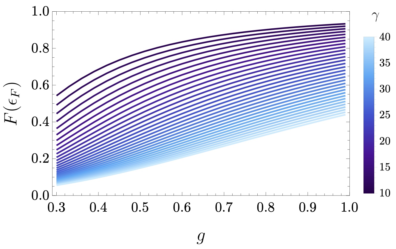
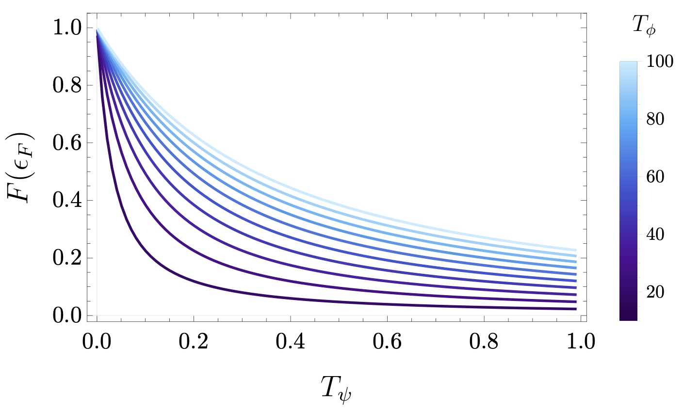
Figure S4: Distribution function at the fermi energy $\epsilon_{F}=\mu$ from the numerical solution of the full non-linear differential equation plotted at $\mu=1=\epsilon_{\textbf{k}}$ for a) fixed $T_{cry}=0.1$, $T_{mir}=100$ while in b) we fix the coupling and dissipation $g=0.5,\gamma=10$ and vary both temperatures

where we defined a new dimensionless constant that parametrices the dissipatio and coupling $\tilde{g}=\sqrt{S_{d-1}}\dfrac{g}{\gamma_{0}^{2}}$. The numerical solution of 6 for more generic temperatures is used in the main text and additonally more features can be seen in Fig. S4.

To arrive at the previous equation the limit where the previous analysis works is when $\nu_{0}/T_{mir}\approx 0$. The crossover point where the distribution function tends to be just the non-interacting one with the electron bath temperature occurs when the terms in the numerator are of equal magnitude. The distribution function becomes generically non thermal but around the Fermi energy if one assumes $F(\mu)=0$ then we see still the photon temperature dominates independent of any coupling constants since the previous differential equation implies:

$$\dfrac{\partial F(\textbf{k},\omega\approx\mu)}{\partial\omega}\approx\dfrac{1}{2T_{mir}}.$$ (S82)

The energy scale when the approximations made no longer gives an accurate picture can be obtained by considering when the electron width and photon width are similar since then one no longer can assume that one distribution dominates. We demand consistency meaning $\absolutevalue{\gamma_{ph}(\tilde{\omega}-\omega)}\ll\absolutevalue{\gamma\tilde{\omega}}$. If we probe at an energy $\omega\approx\omega_{0}+\Delta\epsilon$ then this means the spectral densities of the electrons and photon would be evaluated at distinct frequencies, we demand $\absolutevalue{\gamma_{ph}(\tilde{\omega}-(\omega_{0}+\Delta\epsilon))}\ll\absolutevalue{\gamma(\omega_{0}+\Delta\epsilon\pm\nu_{0})}$ where because of the approximation of $\gamma\gg\gamma_{ph}$ we have $\tilde{\omega}\approx\omega\pm\nu_{0}$ thus the approximation is consistent if:

$$\absolutevalue{\gamma_{ph}(((\omega_{0}+\Delta\epsilon)\pm\nu_{0})-(\omega_{0}+\Delta\epsilon))}\ll\absolutevalue{\gamma(\omega_{0}+\Delta\epsilon\pm\nu_{0})}\quad\Rightarrow\quad\dfrac{\gamma_{ph}}{\gamma}\nu_{0}\ll\absolutevalue{\omega_{0}+\Delta\epsilon\pm\nu_{0}},$$ (S83)

in the case of $\nu_{0}$ large we see that $\omega_{0}=0$ satisfies the consistency condition as long as $\Delta\epsilon$ is small since $\gamma_{ph}/\gamma\ll 1$.

S3.2 Observables

The consequences of the non-thermal steady state will generally manifest on the level of observables via a modified Sommerfeld expansion. We can derive this from considering the expectation value of a single particle observable $\expectationvalue{\hat{O}}$ of the generic form:

$$\expectationvalue{\int dt\sum_{\textbf{k}}o_{\textbf{k}}(t)\psi_{\textbf{k}}(t)^{\dagger}\psi_{\textbf{k}}(t)}=\sum_{\textbf{k}}\int dt\dfrac{o_{\textbf{k}}(t)}{2}\left(iG_{\textbf{k}}^{K}(t)-1\right)=\sum_{\textbf{k}}\int dt\int\dfrac{\differential\omega_{1}}{2\pi}\dfrac{o_{\textbf{k}}(\omega_{1})}{2}e^{i\omega_{1}t}\left(\int\dfrac{\differential\omega_{2}}{2\pi}iG_{\textbf{k}}^{K}(\omega_{2})e^{i\omega_{2}t}-1\right),$$ (S84)

where we used the identity of the Keldysh green’s function $iG^{K}=2\expectationvalue{\psi^{\dagger}\psi}+1$ so that now we can use the parametrisation in terms of $F(\omega)$ and the retarded and advanced greens functions to get:

$$\expectationvalue{\hat{O}}=\sum_{\textbf{k}}\dfrac{1}{2}\int\dfrac{\differential\omega}{2\pi}-2\Im{G^{R}_{\textbf{k}}(\omega)}o_{\textbf{k}}(-\omega)F(\textbf{k},\omega)-o_{\textbf{k}}(0)=\sum_{\textbf{k}}\dfrac{1}{2}\int\dfrac{\differential\omega}{2\pi}2\pi\delta(\omega-\epsilon_{\textbf{k}})o_{\textbf{k}}(-\omega)F(\textbf{k},\omega)-o_{\textbf{k}}(0),$$ (S85)

where we assumed that the width of the spectral function $\gamma$ is much smaller than the region where the observable and occupation function vary. To first order this would mean a big electron temperature $T_{cry}\gg\gamma$. Then we would obtain:

$$\expectationvalue{\hat{O}}=\sum_{\textbf{k}}\dfrac{1}{2}o_{\textbf{k}}(-\epsilon_{\textbf{k}})F(\textbf{k},\epsilon_{\textbf{k}})-\dfrac{1}{2}o_{\textbf{k}}(0)=\dfrac{1}{2}\int\dfrac{\differential^{d}\textbf{k}}{(2\pi)^{d}}o_{\textbf{k}}(F(\epsilon_{\textbf{k}})-1)=\dfrac{1}{2}\int\differential\epsilon\ o_{\epsilon}\ D(\epsilon)(F(\epsilon)-1)=\int\differential\epsilon\ H(\epsilon)\dfrac{1}{2}(F(\epsilon)-1),$$ (S86)

where we assumed also $o_{\textbf{k}}=o_{\textbf{k}}(0)=o_{\textbf{k}}(-\epsilon_{\textbf{k}})$ we also used in the last two equalities spherical coordinates and assuming a spherical dispersion to transform to energy space and defined the density of states as $D(\epsilon)$. We obtain then the usual Sommerfeld expansion by identifying $n(\epsilon)=\dfrac{1}{2}(F(\epsilon)-1)$ which is the usual definition of the Fermi distribution function in the thermal state. We have thus reached the usual form of the initial integral before the Sommerfeld expansion is performed. Let us now use the approximate form of the distribution function we found before:

$$\int\differential\epsilon\ H(\epsilon)\dfrac{1}{2}(F(\epsilon)-1)=\int\differential\epsilon\ H(\epsilon)\dfrac{1}{2}(F_{0}(\epsilon)-1)+\int\differential\epsilon\ H(\epsilon)\dfrac{1}{2}\Delta F(\epsilon).$$ (S87)

The first term gives us the typical Sommerfeld expansion while the last term is the correction we obtain for the non-thermal steady state. We use the the same trick as in the normal expansion by using $H(y)=K^{\prime}(y)$ using integration by parts ( note one can apply this since the correction vanishes faster than $K(\epsilon)$ for both $\epsilon\rightarrow\pm\infty$ ) one obtains:

$$\int\differential\epsilon\ H(\epsilon)\dfrac{1}{2}\Delta F(\epsilon)=\int\differential\epsilon\ K^{\prime}(\epsilon)\dfrac{1}{2}\Delta F(\epsilon)=-\dfrac{1}{2}\int\differential\epsilon\ K(\epsilon)\Delta F^{\prime}(\epsilon)\approx\int\differential xK(T_{cry}x+\mu)\dfrac{\Delta T}{T_{cry}}\partialderivative{x}\ \dfrac{1}{x-1/\tilde{g}^{2}}$$ (S88)

$$=-\int\differential x\sum_{n}\dfrac{1}{n!}K^{(n)}(\mu)(T_{cry}x)^{n}\dfrac{\Delta T}{T_{cry}}\dfrac{1}{(x-1/\tilde{g}^{2})^{2}}\approx-K(\mu)\dfrac{\Delta T}{T_{cry}}\int\differential x\dfrac{1}{(x-1/\tilde{g}^{2})^{2}}-K^{\prime}(\mu)\dfrac{\Delta T}{2}\int\differential x\dfrac{x}{(x-1/\tilde{g}^{2})^{2}}+\dots$$ (S89)

where we approximated to first order in the frequency and introduced a dimensionless parameter $x=\dfrac{\omega-\mu_{0}}{T_{cry}}$ since the functional form is only valid for the linearized problem, we therefore require the integral to range in energy only within a small energy window where $F\approx 0$ which means within $\mu_{0}-T_{cry}$ and $\mu_{0}+T_{cry}$ meaning $x\in(-1,1)$ we have then:

$$\int\differential\epsilon\ H(\epsilon)\dfrac{1}{2}\Delta F(\epsilon)\approx-K(\mu)\dfrac{\Delta T}{T_{cry}}\dfrac{2}{(1/\tilde{g})^{4}-1}-K^{\prime}(\mu)\dfrac{\Delta T}{2}\dfrac{2/\tilde{g}^{2}}{(1/\tilde{g})^{4}-1}\approx-\dfrac{2\Delta T}{T_{cry}}\dfrac{S_{d-1}^{2}g^{4}}{\gamma^{4}}\int_{-\infty}^{\mu}\differential\epsilon\ H(\epsilon)-\Delta T\dfrac{S_{d-1}g^{2}}{\gamma^{2}}H(\mu_{0}).$$ (S90)

We see now that the non-thermal distribution manifests itself in two distinct ways, first a correction to the Fermi distribution at zero temperature which would be just the integral of the observable. Now we get a correction which is linear on the temperature difference and quartic in $g/\gamma$ which by assumption is small. Impressively we also observe a correction proportional to $H(\mu_{0})$ which can’t appear in thermal equilibrium since the derivative of the Fermi distribution is even and cancel every odd term in the expansion of $K(x)$. To lowest order we have a change in the Sommerfeld expansion of the form:

$$\Delta\langle\hat{O}\rangle=(T_{mir}-T_{cry})\dfrac{S_{d-1}g^{2}}{\gamma^{2}}O(\mu)D(\mu).$$ (S91)

A note of caution regarding the chemical potential is in order before studying the case of large photon bath coupling. In the previous calculation we have assumed that the point around which we expand is the non-interacting $\mu_{0}$. One may worry that the actual expansion point is really around the solution of $F(\omega)=0$. This is true in general but if we stick to our physical limits we obtain to lowest order the previous Sommerfeld expansion. To see this we need to consider solving for the energy which fulfills:

$$F_{0}(\mu)+\dfrac{\Delta T}{T_{cry}}\left(\dfrac{1}{\dfrac{\mu-\mu_{0}}{T_{cry}}-\tilde{g}^{-2}}\right)+O(\tilde{g}^{6})=0,$$ (S92)

where as noted before $1/\tilde{g}\gg 1$, now if we had thermal equilibrium then $\mu=\mu_{0}$ and we are done, instead if we are not, the distribution has as seen in eq. 6 a term proportional to $\Delta T*\tilde{g}^{2}\ll 1$ which means corrections to $\mu$ will satisfy $\mu-\mu_{0}\ll 1$ which then allows us to expand the first term $\tanh((\mu-\mu_{0})/(2T_{cry}))$ so as to obtain the equation:

$$\dfrac{\mu-\mu_{0}}{2T_{cry}}\left(\dfrac{\mu-\mu_{0}}{T_{cry}}-1/\tilde{g}^{2}\right)=-\dfrac{\Delta T}{T_{cry}}+O((\mu-\mu_{0})^{4}),$$ (S93)

where the power comes from the expansion of $\tanh$ and the non-thermal correction. Now this is a quadratic equation with solutions:

$$\dfrac{\mu-\mu_{0}}{T_{cry}}=\dfrac{1/\tilde{g}^{2}}{2}\left(1\pm\sqrt{1-\dfrac{8\Delta T}{(1/\tilde{g})^{4}T_{cry}}}\right).$$ (S94)

Only one solution is possible since we know that for $\Delta T\rightarrow 0$ the distribution is thermal and so $\mu=\mu_{0}$ so we have to select the minus sign which will result then on a solution of the form:

$$\mu=\mu_{0}+2\Delta T\tilde{g}^{2}+O((\tilde{g})^{6}).$$ (S95)

As it is clear now the corrections to the chemical potential are indeed smaller, since $\Delta T\tilde{g}^{2}\ll 1$. When included in the Sommerfeld expansion this will give rise to higher order corrections that do not affect our main result. Moreover, we see even from this simple calculation that indeed the chemical potential satisfies the linear in $\Delta T$ prediction from the Sommerfeld expansion, as expected.

Let us now compute the effective temperature when we expand the distribution function on the new chemical potential. For this we expand around $\omega=\mu=\mu_{0}+2\Delta T\tilde{g}^{2}$ which results in :

$$F(\textbf{k},\omega)=F_{0}(\omega)+\dfrac{\Delta T}{T_{cry}}\left(\dfrac{1}{\dfrac{\omega-\mu_{0}}{T_{cry}}-1/\tilde{g}^{2}}\right)\approx\left(\dfrac{1}{2T_{cry}}+\frac{-\Delta T^{2}-\Delta T\ T_{\psi}}{2(1/\tilde{g})^{4}T_{\psi}^{3}}\right)(\omega-\mu)+O((\tilde{g})^{6}).$$ (S96)

We see the correction goes like $(\tilde{g})^{4}$ which means the lowest order Sommerfeld result won’t be affected, additionally we see the effective temperature now gets modifications as a function of $(1/\tilde{g})$ and in general a function of $\nu_{0}$. Moreover it is now possible to define an effective temperature, valid for $\Delta T$ small:

$$T_{eff}\approx T_{cry}+\dfrac{\Delta T(\Delta T+T_{cry})}{(1/\tilde{g})^{4}T_{cry}^{2}}.$$ (S97)

It is worth noting that this effective temperature is not the whole story, if one only uses this and forgets about the non-thermal behaviour of the steady state then one will miss the modified Sommerfeld expansion. The usual Sommerfeld expansion for $T_{eff}$ can never give the observable at the chemical potential $O(\mu)$, the lowest order term is always the integrated observable.

[] []

S3.3 $\gamma_{ph}\gg\gamma$ limit

We now assume that the photons couple strongly to the bath meaning $\gamma_{ph}\gg g^{2}$. We have then that $U^{K}(\textbf{k},\omega)=D_{0}(\omega)(U^{R}_{0}(\textbf{k},\omega)-U^{A}_{0}(\textbf{k},\omega))$. In this case the Keldysh component of the self-energy for the electrons becomes: Additionally if the coupling of the electron bath is not as strong as the photon bath we can assume $\gamma_{ph}\gg\gamma$. In this case the retarded Green’s function minus the advanced Green’s function for the photon is:

$$(U^{R}_{0}(\textbf{k}^{\prime}-\textbf{k},\tilde{\omega}-\omega)-U^{A}_{0}(\textbf{k}^{\prime}-\textbf{k},\tilde{\omega}-\omega))=i\delta(\absolutevalue{\textbf{k}-\textbf{k}^{\prime}})\dfrac{-\gamma_{ph}(\tilde{\omega}-\omega)}{((\tilde{\omega}-\omega)^{2}-\nu_{0}^{2})^{2}+\gamma_{ph}^{2}(\tilde{\omega}-\omega)},$$ (S98)

where we have assumed a separation of the $\gamma_{ph}$ function into a part proportional to the frequency and a function of the momenta which we will take as a constant in the following and absorb it in a prefactor. We have also assumed $\tilde{\omega}-\omega\neq 0$ for a form for $\gamma_{ph}$ such that $\gamma_{ph}(\omega=0)=0$ and so for $\tilde{\omega}-\omega=0$ the spectral function is just zero, in the following equation this condition is assumed. while for the Green’s function of the electrons we expect a sharp localization around the single particle energies in the regime of $g\ll\gamma\ll\gamma_{ph}$ meaning:

$$(G^{R}(\textbf{k}^{\prime},\tilde{\omega})-G^{A}(\textbf{k}^{\prime},\tilde{\omega}))\approx-2\pi i\delta(\tilde{\omega}-\epsilon_{\textbf{k}^{\prime}}),$$ (S99)

which would imply a QKE of the form :

$$2i\gamma(\textbf{k},\omega)(F_{0}(\omega)-F(\textbf{k},\omega))=ig^{2}\int\differential^{d}\textbf{k}^{\prime}\int\differential\tilde{\omega}\ 2\pi i\delta(\tilde{\omega}-\epsilon_{\textbf{k}^{\prime}})i\delta(\absolutevalue{\textbf{k}-\textbf{k}^{\prime}})\dfrac{\gamma_{ph}(\tilde{\omega}-\omega)}{((\tilde{\omega}-\omega)^{2}-\nu_{0}^{2})^{2}+\gamma_{ph}^{2}(\tilde{\omega}-\omega)}H(\tilde{\omega})$$ (S100)

$$\gamma(\textbf{k},\omega)(F_{0}(\omega)-F(\textbf{k},\omega))=-\pi g^{2}S_{d-1}\dfrac{\gamma_{ph}(\epsilon_{\textbf{k}}-\omega)}{((\epsilon_{\textbf{k}}-\omega)^{2}-\nu_{0}^{2})^{2}+\gamma_{ph}^{2}(\epsilon_{\textbf{k}}-\omega)}H(\epsilon_{\textbf{k}})$$ (S101)

$$F_{0}(\omega)-F(\textbf{k},\omega)=\dfrac{-\pi g^{2}S_{d-1}}{\gamma(\textbf{k},\omega)}\dfrac{\gamma_{ph}(\epsilon_{\textbf{k}}-\omega)\left(F(\textbf{k},\epsilon_{\textbf{k}})D_{0}(\epsilon_{\textbf{k}}-\omega)-F(\textbf{k},\omega)(D_{0}(\epsilon_{\textbf{k}}-\omega)-F(\textbf{k},\epsilon_{\textbf{k}}))-1\right)}{((\epsilon_{\textbf{k}}-\omega)^{2}-\nu_{0}^{2})^{2}+\gamma_{ph}^{2}(\epsilon_{\textbf{k}}-\omega)}.$$ (S102)

If we now solve for the frequency dependent distribution function we obtain again a generally non-thermal distribution function:

$$F(\textbf{k},\omega)=\dfrac{\pi g^{2}S_{d-1}\gamma_{ph}(\epsilon_{\textbf{k}}-\omega)(1-F_{0}(\epsilon_{\textbf{k}})D_{0}(\epsilon_{\textbf{k}}-\omega))-\gamma(\omega)L(\omega)F_{0}(\omega)}{\pi g^{2}S_{d-1}\gamma_{ph}(\epsilon_{\textbf{k}}-\omega)(F_{0}(\epsilon_{\textbf{k}})-D_{0}(\epsilon_{\textbf{k}}-\omega))-\gamma(\omega)L(\omega)}.$$ (S103)

we now approximate the function around a point not at the electron energy for example around $\omega=\dfrac{\epsilon_{\textbf{k}}}{2}$ and noting that $F(\textbf{k},\epsilon_{\textbf{k}})=F_{0}(\epsilon_{\textbf{k}})$ since the right hand side of equation (S98) vanishes for $\omega=\tilde{\omega}=\epsilon_{\textbf{k}}$. For large $\gamma_{ph}$ we obtain then:

$$F(\textbf{k},\omega)\approx F_{0}\left(\dfrac{\epsilon_{\textbf{k}}}{2}\right)+\left(1-F_{0}\left(\dfrac{\epsilon_{\textbf{k}}}{2}\right)^{2}\right)\dfrac{\omega-\dfrac{\epsilon_{\textbf{k}}}{2}}{2T_{cry}},$$ (S104)

which means that locally probing energies smaller than the electron energy again results in an approximate thermal distribution with the electron bath temperature. From the previous section arguments we can also deduce the frequencies for which the opposite limit $\gamma_{ph}\gg\gamma$ is consistent with the approximation of a delta function in the electron spectral density meaning $\tilde{\omega}\approx\epsilon_{\textbf{k}}$ since it will break down for :

$$\absolutevalue{\gamma_{ph}(\epsilon_{\textbf{k}}-\omega)}\approx\absolutevalue{\gamma\omega}\quad\Rightarrow\quad\omega\approx\dfrac{\gamma_{ph}}{\gamma+\gamma_{ph}}\epsilon_{\textbf{k}},$$ (S105)

which means the approximation is consistent as long as one expands around $\omega\ll\dfrac{\gamma_{ph}}{\gamma+\gamma_{ph}}\epsilon_{\textbf{k}}\approx\epsilon_{\textbf{k}}$.

References

von Klitzing et al. [2020]K. von
Klitzing, T. Chakraborty, P. Kim,
V. Madhavan, X. Dai, J. McIver, Y. Tokura, L. Savary, D. Smirnova, A. M. Rey, C. Felser, J. Gooth, and X. Qi, 40 years of the quantum hall effect, Nature Reviews Physics 2, 397 (2020).
Mackenbach et al. [2022]R. J. J. Mackenbach, J. H. E. Proll, and P. Helander, Available energy of trapped electrons and its relation to turbulent
transport, Phys. Rev. Lett. 128, 175001 (2022).
Ren et al. [2022]L. Ren, L. Lombez,
C. Robert, D. Beret, D. Lagarde, B. Urbaszek, P. Renucci, T. Taniguchi, K. Watanabe, S. A. Crooker, and X. Marie, Optical
detection of long electron spin transport lengths in a monolayer
semiconductor, Phys. Rev. Lett. 129, 027402 (2022).
Needleman and Dogic [2017]D. Needleman and Z. Dogic, Active matter at the
interface between materials science and cell biology, Nature Reviews Materials 2, 17048 (2017).
Xi et al. [2019]W. Xi, T. B. Saw,
D. Delacour, C. T. Lim, and B. Ladoux, Material approaches to active tissue mechanics, Nature Reviews Materials 4, 23 (2019).
Foglino et al. [2019]M. Foglino, E. Locatelli,
C. A. Brackley, D. Michieletto, C. N. Likos, and D. Marenduzzo, Non-equilibrium effects of molecular motors on polymers, Soft Matter 15, 5995 (2019).
Lemoult et al. [2016]G. Lemoult, L. Shi,
K. Avila, S. V. Jalikop, M. Avila, and B. Hof, Directed percolation phase transition to sustained turbulence in
couette flow, Nature Physics 12, 254 (2016).
Oberlack et al. [2022]M. Oberlack, S. Hoyas,
S. V. Kraheberger,
F. Alcántara-Ávila, and J. Laux, Turbulence statistics of arbitrary moments of
wall-bounded shear flows: A symmetry approach, Phys. Rev. Lett. 128, 024502 (2022).
Siegman [1986]A. E. Siegman, Lasers (University science books, 1986).
Garcia-Vidal et al. [2021]F. J. Garcia-Vidal, C. Ciuti, and T. W. Ebbesen, Manipulating matter by
strong coupling to vacuum fields, Science 373, (2021).
Mivehvar et al. [2021]F. Mivehvar, F. Piazza,
T. Donner, and H. Ritsch, Cavity qed with quantum gases: new paradigms in many-body
physics, Advances in Physics 70, 1 (2021).
Bloch et al. [2022]J. Bloch, A. Cavalleri,
V. Galitski, M. Hafezi, and A. Rubio, Strongly correlated electron–photon systems, Nature 606, 41 (2022).
De La Torre et al. [2021]A. De La Torre, D. M. Kennes, M. Claassen,
S. Gerber, J. W. McIver, and M. A. Sentef, Colloquium: Nonthermal pathways to ultrafast control in
quantum materials, Reviews of Modern Physics 93, 041002 (2021).
Curtis et al. [2019]J. B. Curtis, Z. M. Raines,
A. A. Allocca, M. Hafezi, and V. M. Galitski, Cavity quantum eliashberg enhancement of
superconductivity, Physical review letters 122, 167002 (2019).
Chakraborty and Piazza [2021]A. Chakraborty and F. Piazza, Long-range photon
fluctuations enhance photon-mediated electron pairing and
superconductivity, Phys. Rev. Lett. 127, 177002 (2021).
Chakraborty and Piazza [2022]A. Chakraborty and F. Piazza, Controlling collective
phenomena by engineering the quantum state of force carriers: The case of
photon-mediated superconductivity and its criticality, arXiv preprint 10.48550/arXiv.2207.07131
(2022).
Eckhardt et al. [2023]C. J. Eckhardt, S. Chattopadhyay, D. M. Kennes, E. A. Demler,
M. A. Sentef, and M. H. Michael, Theory of resonantly enhanced
photo-induced superconductivity, arXiv preprint 10.48550/arXiv.2303.02176 (2023).
Viñas Boström et al. [2023]E. Viñas Boström, A. Sriram, M. Claassen, and A. Rubio, Controlling the magnetic state of the proximate
quantum spin liquid -rucl3 with an optical cavity, npj Computational Materials 9, 202 (2023).
Jarc et al. [2023]G. Jarc, S. Y. Mathengattil, A. Montanaro, F. Giusti,
E. M. Rigoni, R. Sergo, F. Fassioli, S. Winnerl, S. Dal Zilio, D. Mihailovic, et al., Cavity-mediated thermal control of metal-to-insulator
transition in , Nature 622, 487 (2023).
Chiriacò [2023]G. Chiriacò, Thermal purcell
effect and cavity-induced renormalization of dissipations, arXiv preprint 10.48550/arXiv.2310.15184
(2023).
Eliashberg [1970]G. Eliashberg, Film
superconductivity stimulated by a high-frequency field., Tech. Rep. (Inst. of Theoretical Physics,
Moscow, 1970).
Sieberer et al. [2015]L. M. Sieberer, A. Chiocchetta, A. Gambassi, U. C. Täuber, and S. Diehl, Thermodynamic equilibrium
as a symmetry of the schwinger-keldysh action, Phys. Rev. B 92, 134307 (2015).
Kamenev [2023]A. Kamenev, Field theory of
non-equilibrium systems (Cambridge University
Press, 2023).
Schlawin et al. [2019]F. Schlawin, A. Cavalleri, and D. Jaksch, Cavity-mediated
electron-photon superconductivity, Phys. Rev. Lett. 122, 133602 (2019).
Andolina et al. [2022]G. M. Andolina, A. De Pasquale, F. M. D. Pellegrino, I. Torre,
F. H. Koppens, and M. Polini, Can deep sub-wavelength cavities induce amperean
superconductivity in a 2d material?, arXiv preprint 10.48550/arXiv.2210.10371
(2022).
Piazza and Strack [2014]F. Piazza and P. Strack, Quantum kinetics of
ultracold fermions coupled to an optical resonator, Physical Review A 90, 043823 (2014).
Rao and Piazza [2023]P. Rao and F. Piazza, Non-fermi-liquid behavior from cavity
electromagnetic vacuum fluctuations at the superradiant transition, Phys. Rev. Lett. 130, 083603 (2023).
Supplemental material for “Non-thermal electron-photon steady-states in open cavity-quantum-materials”
R. Flores-Calderón,1,∗ Francesco Piazza,1,2
1 Max Planck Institute for the Physics of Complex Systems, Nöthnitzer Strasse 38, 01187 Dresden, Germany
2Theoretical Physics III, Center for Electronic Correlations and Magnetism,
Institute of Physics, University of Augsburg, 86135 Augsburg, Germany
∗Electronic address: rflorescalderon@pks.mpg.de
(Dated: )