Long-term evolution in ionization of ejecta illuminated by Eta Carinae

Abstract

Changes in the flux and spectrum of Eta Carinae since 1900 have been attributed to the evolution of the central binary by some. Others suggest evolution in the occulting ejecta. The brightness jump in the 1940s, which coincided with the appearance of narrow forbidden emission lines, may have been caused by the clearing and ionization of intervening circumstellar ejecta. The brightening changed at a slower pace up through forty years later. Here we continue earlier studies focused on the long-term showing that the forbidden line emission increased in the early 1990s with no noticeable increase in the brightness of the Homunculus. We interpret that the increase in narrow line emission is due to decreased extinction in the LOS from the central binary to the Weigelt clumps. In 2000, the central stellar core increased in brightness at a faster rate without associated changes in the Homunculus. By 2018, hundreds of narrow-line absorptions from singly-ionized metals in our LOS from Eta Carinae disappeared, thought to be caused by increased ionization of metals. These three events (1990, 2000, and 2018) are explained by the dissipation of circumstellar material within the Homunculus close to the binary. Combining these changes with the steadiness of the Homunculus and the primary winds over the past four decades indicates that circumstellar ejecta in our direction have been cleared.

1 Introduction

Eta Carinae ($\eta$ Car) is the best-observed example of a very massive stellar object in the local Milky Way. It became famous for its 1840s Great Eruption (GE) and the 1890s Lesser Eruption (LE), which are still not well understood (Davidson & Humphreys, 1997; Smith, 2008). By the 1900s, $\eta$ Car was frequently monitored with its photometric variabilities and complex spectra which only reinforced its reputation as an unstable, unpredictable star (Mehner et al., 2010b; Fernández-Lajús et al., 2009; Hirai et al., 2021). Doubly-ionized, forbidden lines appeared in the 1940s (Gaviola, 1953) probably because of the dissipation in the circumstellar ejecta close to $\eta$ Car. The Weigelt knots and the surrounding ejecta became directly bathed by the radiation of the star. The forbidden doubly ionized lines at intervals briefly disappeared with singly-ionized lines remaining. Archival analysis of spectra led to the discovery of the binary period based on the months-long low-ionization events (Damineli, 1996). $\eta$ Car was found to be an eccentric, massive binary system (Damineli et al., 1997, 2000; Corcoran et al., 2017; Grant et al., 2020; Strawn et al., 2023). The hot secondary provides the high-ionization photons leading to the doubly-ionized narrow lines which disappear while the secondary star plunges into the extended, dense wind of the primary across the periastron.

The discovery of the near knot-like Weigelt clumps (Weigelt & Ebersberger, 1986; Hofmann & Weigelt, 1988), projected to be $\sim$ 0$\farcs$3 from $\eta$ Car, soon were understood to be slowly moving clumps of ejecta. Spectroscopy of the Weigelt clumps, resolved from $\eta$ Car, demanded sub-arcsec spatial resolution, accessible only by HST. Davidson et al. (1995) demonstrated that Weigelt D and B were sources of the narrow high-ionization forbidden lines that offered a means to monitor the central binary and to model the luminosity and temperature of the secondary star (Verner et al., 2002, 2005; Mehner et al., 2010a; Teodoro et al., 2020).

The apparent long-term spectral evolution of $\eta$ Car had been attributed to intrinsic variations, such as a decrease in the mass-loss rate of the primary star or evolution of a latitudinal-dependent stellar wind (Mehner et al., 2015; Smith et al., 2003). However, intrinsic wind changes conflict with observational results, such as $a)$ the stable, long-term, near-infrared and mid-infrared luminosity from 1968 to 2018 (Mehner et al., 2019); $b)$ the steadily repeating X-ray light curve over multiple binary orbits (Corcoran et al., 2017; Espinoza Galeas et al., 2021); $c)$ the constancy of the dust-scattered spectrum from the Homunculus (Hillier & Allen, 1992; Damineli et al., 2021), d) the constancy of the reflected continuum flux in Weigelt D in a period when the star brightened (Mehner et al., 2012) and $e)$ the repeatability of the narrow line fluxes from the ejecta. Regarding the Homunculus brightness, Smith (2017) examined two images taken by HST in 1995 and 1998 and found a brightness difference of 34 %. In the long term, however, the nebular brightness is flat, with excursions up to 0.3 mag from the average 5.6ṁag in the F550M filter of the ACS/HRC HST camera. See Fig. 5 and Table A1 of Damineli et al. (2019)

Hillier & Allen (1992) first suggested that an occulter must be in our LOS to $\eta$ Car. Its impact on the photometric and spectroscopic evolution of $\eta$ Car was further discussed by Damineli et al. (2019, 2021, 2023) and Pickett et al. (2022). In addition, Gull et al. (2023) showed that, between 2004 and 2018, many singly-ionized absorption lines disappeared across an extended portion of the Homunculus (within $\pm$ 1$\farcs$5 of the central stellar core), indicating that the dissipating occulter extended well beyond our LOS to $\eta$ Car.

Humphreys et al. (2008) reported the spectroscopic and photometric evolution of $\eta$ Car, showing that the star was photometrically stable in the period from 1900 to 1940. The spectrum also remained nearly constant over that period, displaying only low excitation lines like H i, Fe ii and [Fe ii]. In the period 1940–53 there was an episode of brightening, which was in coincidence with the appearance of He i and [Fe iii] lines. The object slowly brightened up to the 1990s, the [Fe iii]/[Fe ii] ratio increased, while the He i remained at a roughly constant level. To understand the evolution of $\eta$ Car recently, two main questions need to be properly addressed: how have the spectral and photometric variations evolved in the last three decades? What caused the remarkable events that occurred around the 1940s and 1990s?

To obtain more insight on this subject, we collected about 500 high-resolution spectra covering the last three decades (see, e.g., Damineli et al. 2021, 2023). We used them to analyze the evolution of the degree of ionization of the ejecta clumps by measuring the peaks of the narrow lines Fe ii $\lambda 4631$, [Fe ii] $\lambda 4641$, and [Fe iii] $\lambda 4659$. The last line is sensitive to photoionization, probing the amount of radiation from the secondary star received by the ejecta while the first two lines are largely supported by the primary stellar UV shortward of Lyman $\alpha$. The electron density of the clumps is sufficiently high (log,N_e $\sim$ 7) to cause the [Fe ii] $\lambda 4641$ emission to be dominated by collisional processes and almost insensitive to the radiation field (Mehner et al., 2010a; Teodoro et al., 2020).

The reader will note that the ionization potentials (IPs) of Fe to Fe⁺ is 7.90 eV and Fe$+$ to Fe⁺⁺ is 16.18 eV. With H to H⁺ at 13.6 eV, the [Fe ii] and [Fe iii] discriminate between the presence of radiation above and below the ionization of hydrogen.

In this scenario, the excitation of Weigelt B and D was discussed by Verner et al. (2002, 2005). Gull et al. (2016) described spatially resolved maps of [Fe ii] $\lambda$4815 and [Fe iii] $\lambda$4659 in detail. Mehner et al. (2010a) discussed the variability of the [Fe iii $\lambda$4659 lines for Weigelt D across orbital cycle 10. Gull et al. (2016) and Teodoro et al. (2020) discussed the changes in the mapped forbidden lines across cycle 12. There were a few intrinsic cycle-to-cycle changes in the line emission, especially the disappearance in Weigelt B between cycle 10 and cycle 12 (Gull et al., 2016), but without a substantial impact on the narrow-line emission fluxes. The [Fe iii] $\lambda 4659$ line changes dramatically across both orbital cycles, complicating the study of its long-term evolution without accurate comparisons at the same phases in different cycles, which motivated us to conduct the present work.

The trade-off from monitoring with ground-based spectrophotometry versus HST/STIS is losing all spatial- and velocity-field details to focus on the narrow line peaks with dense time sampling over many orbital cycles. We chose to use frequent high-resolution, ground-based spectroscopy to monitor the ionization of all ejecta clumps over the last six orbits, based on the fluxes of the Fe ii $\lambda 4631$, [Fe iii] $\lambda 4641$ and [Fe ii] $\lambda 4659$ lines.

The selection of these three iron lines was motivated by their wavelength proximity, sharing a common stellar continuum, and the fact that two of them - [Fe iii] $\lambda 4659$ and [Fe ii] $\lambda 4641$ - have been reported since the 1940s and their ratio is sensitive to the degree of ionization of the nebula.

2 Data: observations and reduction

2.1 Absolute flux of the forbidden emission structure with the HST/STIS

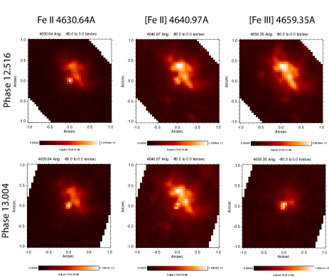
Figure 1: HST/STIS mappings of the emission lines at the high-ionization state, 12.516, and at the low-ionization state, 13.003. The Fe ii $\lambda$4631 and the [Fe ii] $\lambda$4641 structures and intensities change minimally from high-ionization to low-ionization states. The [Fe iii] $\lambda$4659 fluxes drop during the periastron passage as $\eta$ Car-B is immersed within the extended wind of $\eta$ Car-A. The residual flux in the [Fe iii] 4659Å map at 13.004 is from [Co ii] 4658.94$\AA$ and [Fe ii] 4658.29$\AA$. The angular resolution is 0$\farcs$1 and the velocity is centered at $-$40 km s^-1, the velocity of the Weigelt clumps with a width of 80 km s^-1. The intensity display is sqrt(flux).

Diffraction-limited mappings of selected emission lines had been obtained using the Hubble Space Telescope /Space Telescope Imaging Spectrograph (HST/STIS) across one cycle of the $\eta$ Car 5.53-year period. As Gull et al. (2016) addressed changes in the structures of [Fe ii] $\lambda$4815 compared to [Fe iii]$\lambda 4659$, we revisited the data to directly compare [Fe ii] $\lambda$4641 with [Fe iii] $\lambda$4659.

The mappings of Fe ii $\lambda$4631, [Fe ii] $\lambda$4641 and [Fe iii] $\lambda$4659 are compared in Figure 1 at the high-ionization state, 12.516, and at the low-ionization state, 13.003. The structure of Fe ii and [Fe ii] changed little between the high- and low-ionization state, but the [Fe iii] drops dramatically by the low-ionization state. Further examination of the individual spectra that were used to build the map of [Fe iii] and with comparison to the spectral atlas published by Zethson et al. (2012) strongly suggests that the weak emission seen in [Fe iii] $\lambda$4659 in the low-ionization state originates from two weak lines of [Fe ii] at 4658.29Å and [Co ii] at 4658.94Å. i.e. likely the [Fe iii] $\lambda$4659 is completely absent during the low-ionization state, consistent with the ionizing photons necessary for Fe⁺⁺ originating from the hot secondary, $\eta$ Car-B, which is enshrouded by the extended primary wind during periastron passage.

Since absolute fluxes are precious information, we searched the HST/STIS database for visits separated by one or more cycles at the same orbital phase. We found just a pair of spectra centered on the Weigelt D knot, covering the three iron lines that we are focusing on - see Figure 2. The STIS spectra were taken with the slit width $\sim$ 0$\farcs$1 and extracted in a window $\sim$ 0$\farcs$125 long. The slit PA orientation was different for the two visits, which may cause an uncertainty of $\sim$ 10% in the absolute flux. The two STIS spectra are just for a sanity check of our ground-based observations, which are subject to more complex factors, such as $a)$ knot D is $\sim$ 70% stronger than C at this phase (Teodoro et al., 2020), $b)$ ground-based observations correspond to even larger line fluxes because a larger area is sampled due to the slit width, $d)$ ground-based spectra sample clumps with different physical conditions, resulting in different line ratios as compared to the single knot D observed by STIS.

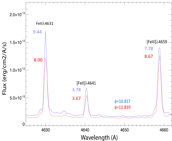
Figure 2: Spectra extracted from HST/STIS observations centered upon Weigelt D at phases 10.817 and 12.839 demonstrate minimal changes in the interval between cycles 10 and 12, consistent with ground-based spectrophotometry in Fig. 4. Numbers near the peaks indicate continuum-normalized intensities. They are larger than in ground-based spectra because of the lower continuum flux at better spatial resolution.

2.2 High-spectral resolution ground-based spectroscopy from cycle-to-cycle

Using multiple ground-based spectrographs we gathered spectra with a signal-to-noise ratio of 100–500 and spectral resolving power ranging from R $\sim$90 000 to 22,000 (see Table 1 for the origin of the spectra). Many of these spectra have been used in several recent papers by our group which details the reductions of the data (see, e.g., Richardson et al., 2010, 2015, 2016; Teodoro et al., 2016; Damineli et al., 2008, 2019, 2021, 2023; Pickett et al., 2022; Strawn et al., 2023) The spectra were normalized by using a linear fit through the pseudo continuum in the range 4550–4750 Å. Even though faint lines present in these spectral windows could introduce a source of error in the normalized intensity of the lines, the main source of scattering in the line intensities is due to different spectral resolutions and differences in seeing conditions. The signal-to-noise exhibits a more significant impact for the line [Fe ii] $\lambda 4641$, which is relatively faint, than for the other two stronger lines, except for [Fe iii] $\lambda 4659$ across the low-excitation periastron passages.

Table 1: Observatories

Observ.	Telescope	R	number
	aperture		measur.
LCOGT/NRES	1 m	48 k	212
CTIO/CHIRON	1.5 m	80 k	196
ESO/FEROS	1.5&2.2 m	48 k	109
LNA/OPD	1.6 m	22 k	47
ESO/Hexapod	1.5 m	48 k	3
ESO/UVES	8 m	90 k	15
Mount Strom. Obs.	1 m	48 k	7
B. Heatcote	0.28 m	16 k	1

Differences in spectral resolution can impact the intensities since we are measuring narrow lines, especially Fe ii $\lambda 4631$ which is the narrowest with fwhm $=$53 km s^-1, as compared to 58 km s^-1 for [Fe iii] $\lambda 4641$ and 84 km s^-1 for [Fe iii] $\lambda 4659$.

Most of the line and continuum flux originates in a region inside a $\sim$ 0$\farcs$5 radius. The seeing smears out the image to $\sim$1–3^′′, so there is not much difference between slit or fiber-fed spectrographs. An exception was noticed in a few of the UVES spectra which used a (0$\farcs$2 aperture) under excellent seeing conditions. The scatter cancels out very nicely through line ratios.

The decreasing strength in the emission lines (see Fig. 3 in Mehner et al. 2015) is not intrinsic, but due to the contrast between the forming region (Weigelt clumps) and the central star brightness which increases as the intervening occulter dissipates (Damineli et al., 2021). But this dominant effect masks long-term intrinsic evolution. The Fe ii $\lambda 4631$ was the strongest in 1997.0 but in 2023.6, it had its peak intensity lower than that of [Fe iii] $\lambda 4659$. Labels in black indicate the peaks of the line intensities. The lines were normalized to the continuum flux and displaced vertically for clarity. Phase is calculated using P $=$ 2022.7 days and $\phi$ $=$ 14.0 is for 2020.2.

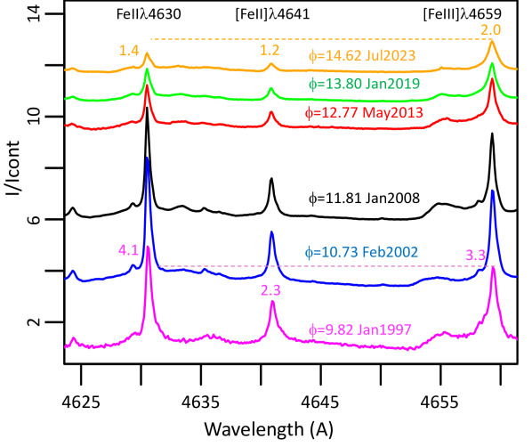
Figure 3: Ground-based evolution of continuum-normalized line intensity of three narrow iron lines. The increase in the continuum flux of the whole object (Homunculus + stellar core) is the cause of the general decrease with time of the normalized line intensities. As shown in Figure 2, the flux in the Weigelt knots is reasonably constant. The evolution of the line strengths is exemplified by the numbers near the line peaks.

We linked the modern records of the [Fe iii] $\lambda 4659$ $/$ [Fe ii] $\lambda 4641$ ratio to six spectra recorded on photographic plates and one spectrophotometric scan recorded before the 1990s. Photographic plates have a logarithmic response on top of an unknown background threshold. The uncertainty in correcting photographic plate responses was challenging for the six photographic spectra - Table 2.

For the spectra reported by Humphreys et al. (2008) and Zanella et al. (1984), we measured the line intensities in the plotted scan and applied a logarithmic correction to derive the line ratio.The measurement for the 1938 ratio - Figure 10 in (Humphreys et al., 2008) - is very uncertain as the [Fe iii] $\lambda 4659$ is exceedingly faint. However, the identification of [Fe iii] $\lambda 4659$ seems to be correct because [Fe iii $\lambda 4702$], although much fainter is clearly present. We adopted a generous upper limit of 0.3 for this ratio. Gaviola’s spectra indicated a level almost three times higher just one cycle ahead at the same phase. We used the reported intensities of the spectra presented by Gaviola (1953) and Thackeray (1953).

The measure of line intensities by Aller (1966) was calibrated with photoelectric scans. The spectrum reported by Hillier & Allen (1992) was recorded with a CCD, and our measurement is very close to those reported in Table 2 of Humphreys et al. 2008. We adopt the values of those authors for the four measurements in common.

Our experiments with modern spectra indicate that this ratio is affected by the spectral resolution although by a reasonable, predictable amount.

The V$-$band light curve was collected from many sources - especially Smith & Frew (2011) and Frew (2004) - and assembled by doing small zero-point shifts to bring the magnitudes (Fernández-Lajús et al., 2009; Damineli et al., 2019) to the same scale as the La Plata monitoring campaign (http://etacar.fcaglp.unlp.edu.ar/EtaCar/). Most of these measurements were extracted inside a circular-aperture radius of 12  arcsec (Fernández-Lajús et al., 2009) in a differential-magnitude scheme, using HDE303308 as a comparison and resulting in an accuracy of $\sim$ 0.01 mag. In addition to the V$-$band photometry, we used the TG bandpass reported in AAVSO (https://www.aavso.org/), which conforms nicely with the V$-$band after a small shift in the zero-point.

All the facilities are listed in Table 1 and the corresponding observational programs are provided in the Acknowledgements.

3 Results

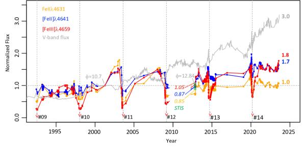
Figure 4: Time series of the three iron lines in the last 30 years. Line intensities are multiplied by the V$-$band flux (gray line). All fluxes are normalized to the unit value in 2002.1, ($\phi$ $=$ 10.7) - gray label. This phase and $\phi$ $=$ 12.8 correspond approximately to dates when the STIS spectra in Fig. 2 were taken. STIS fluxes at $\phi$ $=$ 12.839 relative $\phi$ $=$ 10.817 are indicated in italics in cycle 12 - small green rectangle. The STIS fluxes over these three cycles are $\sim$ 10% higher than those taken with ground-based spectra. Labels to the right of each time series indicate the value in 2023.6. Labels at the bottom, placed near the vertical dashed lines, indicate the running number of low-excitation events.

3.1 Line-flux evolution from cycle to cycle

The line-intensity fluxes of the three iron lines observed by STIS shown in Figure  2 (blue for $\phi$ $=$ 10.817 and red for $\phi$ = 12.839) are much more prominent than in ground-based spectra (Figure 3) at the same phases because STIS probes much fainter continuum flux at better spatial resolution. Except for the Fe ii line, which seems roughly fainter at $\phi$ $=$ 12.839, the two forbidden lines remained at the same flux within the uncertainties. The [Fe iii] $\lambda 4659$ $/$ [Fe ii] $\lambda 4641$ flux ratio remained reasonably constant for the same phase separated by three cycles. The reader should note that Figure 2 presents the spectrum of Weigelt D only, not of the entire group of emission clumps.

For ground-based observations, the most evident evolutionary pattern of the continuum-normalized, narrow iron emission lines is a generally strong fading with time, as shown in Fig. 3. The dates of the spectra were chosen to be in high-excitation phases ($\phi$ $\sim$ 0.6–0.8) when intensity variations along the cycle are relatively small. These lines suffer a significant fading factor over a long time scale because $1)$ the stellar continuum is increasing as the extinction of the occulter along our LOS to the stellar core is decreasing, and $2)$ the clumps are located outside of that region of extinction, which is consistent with the decreasing intensity observed for the Fe ii $\lambda 8610$ line (Damineli et al., 2023). In addition to the general weakening of the line intensities, the ratio between the line peaks of [Fe iii] $\lambda 4659$ to Fe ii $\lambda 4631$ changed from 0.8 to 1.4, suggesting that the excitation degree in the ejecta clumps increased with time. Note that this is not related to the contamination of the central source since the continuum is the same for the three lines. If this effect is real, the ejecta clumps are receiving more high-ionization flux now than in the 1940s. Is this due to a decreasing mass loss rate of the primary star or to the partial dissipation of ejecta along the LOS from the Weigelt clumps to the secondary star? In the next sub-sections, we will try to answer these questions by investigating the time series of line intensities.

3.2 Time series of line intensities

Long-term spectral time series encompassing multiple orbital cycles is a key ingredient to obtaining a more comprehensive understanding of the evolution of spectral lines. Since the most prominent component of the lines originated in the ejecta clumps is narrow, high spectral resolving power (R $>$ 20,000) is necessary. The second most important factor in a long-time series is to keep the spectral resolution as constant as possible. The spatial resolution is not a key factor in ground-based observations to intercompare line intensities from different spectrographs since a slit or a fiber sample the inner 1–3$\farcs$5 diameter around the source, where most of the continuum is formed. Most of the nebula does not contribute to the stellar continuum. The full list of the spectral measurements analyzed in this section is presented in Table 4.

Table 2: Line peak intensity ratio of [Fe iii]$\lambda 4659$/[Fe ii]$\lambda 4641$, measured at different epochs and orbital phases of the $\eta$ Car system.

Year	Phase	Ratio	comm.	Reference
1938	-0.85	$<$ 0.3	–	H08
1944	0.24	0.8	–	G53
1951.22	1.54	0.7	–	T53
1961.25	3.35	1.00	–	A66
1974.08	5.67	1.05	–	Z84
1983.13	7.30	1.00	–	Z84
1986.22	7.88	1.15	–	H92
1994.15	9.31	1.30	R=5k	ESO/FEROS
1996.35	9.71	1.65	R=5k	ESO/FEROS
1999.58	10.29	1.32	R=5k	ESO/FEROS
2002.5	10.82	1.40	R=5k	ESO/FEROS
2005.19	11.29	1.33	R=5k	ESO/FEROS
2008.02	11.81	1.43	R=5k	ESO/UVES
2013.30	12.77	1.49	R=5k	CTIO/CHIRON
2016.94	13.42	1.36	R=5k	ESO/FEROS
2019.05	13.82	1.54	R=5k	LCOGT/NRES
2021.24	14.31	1.49	R=5k	LCOGT/NRES
2023.57	14.62	1.44	R=5k	LCOGT/NRES
2002.6	10.82	2.06	Weigelt D	HST/STIS
2013.8	12.84	2.36	Weigelt D	HST/STIS

Notes: References: H92=Hillier & Allen (1992); H08=Humphreys et al. (2008); G53=Gaviola (1953); T53=Thackeray (1953); Z84=Zanella et al. (1984); R = 5 000 - degraded resolution to compare with 1938-86 ratio.

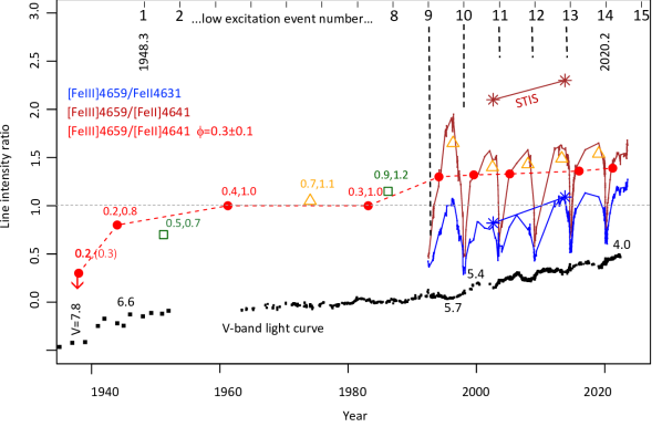
Figure 5: Iron line ratios estimated from the continuum-normalized spectra. Ground-based measures of the [Fe iii] $\lambda 4659$ $/$ [Fe ii] $\lambda 4641$ ratio are represented by small brown dots reported in Table 4. The blue line represents the flux ratio [Fe iii] $\lambda 4659$ $/$  Fe ii $\lambda 4631$. Brown and blue asterisks represent STIS measures of the two ratios. The red-filled circles are the ratios after degrading the spectra to R $=$ 5 000 - Table 2. The focus on $\phi$ $=$ 0.3 is to link them with the historical measurements taken at $\phi$ $=$ 0.3 $\pm$ 0.1 also reported in Table 2. Orange triangles indicate line-flux ratios for high excitation phases ($\phi$ $=$ 0.7-0.8) from spectra degraded to R $=$ 5 000. In the upper axis, the times of the low-excitation events are marked (01 is for the first one observed by Gaviola (1953) in 1948.3). The V$-$band light curve is displayed at the bottom (black squares), and the black numbers close to it indicate the magnitude of the whole object (core+Homunculus).

The best strategy to follow the long-term evolution of these three lines - [Fe iii] $\lambda 4659$, [Fe ii] $\lambda 4641$, and Fe ii $\lambda 4631$ - consists of the conversion of their intensities relative to the stellar continuum to relative fluxes, as shown in Fig. 4. The conversion is done by multiplying their intensities by the $V$-band flux light curve (gray line) observed from the ground, which encompasses the entire object (core plus the Homunculus). The absolute flux accuracy is irrelevant since we are dealing with flux ratios.

On top of the secular brightening of the object, some oscillations became more pronounced as the stellar core became dominant over the nebula in the latest cycles. The oscillation amplitude is $\sim$ 0.4  mag due to the variation of the projected shape of the primary’s to our LOS, distorted by the cavity produced by the wind-wind collision when it goes around the orbit. The amplitude of the light-curve oscillation isolating just the stellar core is almost twice the whole object because the Homunculus adds a constant light corresponding to V_H $\sim$ 5.5 mag (see Fig. 16 from Damineli et al. 2019).

The spectral-line time-series and the V$-$band light-curve were normalized to their values at 2002.1 ($\phi$ = 10.7) - Fig. 4. This choice is arbitrary and was selected to be as close as possible to the phase of the spectrum taken with STIS at $\phi$ $=$ 10.817. A second spectrum was taken in the same position (Weigelt D) two cycles later, at phase $\phi$ $=$ 12.839 (Fig. 2). The absolute fluxes measured in Weigelt D show almost no temporal evolution between the two epochs - see Fig. 4. Their relative fluxes are $\sim$ 10 % higher than the corresponding ground-based observations. This demonstrates that the spectrophotometry from the ground recovers the line flux of the ejecta clumps with fairly good accuracy when compared to the analysis of STIS spectroscopy. The two dates when the STIS spectra were taken are shown as gray numbers and marked with a small green rectangle in cycle 12 in Fig. 4.

The behavior of the [Fe iii] $\lambda 4659$ line along the orbital cycles presented in Fig. 4 is in agreement with that discussed by Mehner et al. (2010a) for cycle 10, and by Teodoro et al. (2020) for cycle 12. There is a sharp minimum at phase zero (probably reaching zero intensity) and fast recovery to the high-excitation phases leading to a pronounced peak around phase 0.9 (about three months before phase zero). The situation is similar for the other two iron lines, but their minima do not go to zero intensity, and the mid-cycle maximum is less pronounced. The pre-minimum peak at the end of the cycles is not present in the ratio curve [Fe iii] / [Fe ii] of Fig. 3. This is unexpected since [Fe iii] is sensitive to the ionization flux, but [Fe ii] is not (see, e.g., the discussion for the Weigelt D knot in Teodoro et al. 2020).

The $V$-band flux has increased by a factor of three since 2001 (gray light curve in Figure 4). This flux increase is caused by the dissipation of the occulter along our LOS to the stellar core. The fact that the [Fe iii] flux also increased indicates that more radiation from the ionizing secondary is reaching the ejecta clumps. Moreover, Gull et al. (2023) reported the disappearance of extended narrow absorption structures in yet another direction during the last orbital cycle. These three observational facts indicate that the dissipation process impacts different circumstellar regions at different times.

3.3 Intensity ratio of [Fe iii] to [Fe ii] and to Fe ii lines

Figure 5 presents the line intensity ratio curve derived from Table 4 - blue and brown curves. The Fe⁺⁺ to Fe⁺ ratios are much smoother than the time series presenting the same data as flux intensities for each line. The plot shows a remarkable variation caused by the orbital motion of the central binary, which modulates the ionizing flux impacting on the ejecta clumps. The Fe⁺⁺ line tracks the flux from the secondary star - which plunges into the primary’s wind inner region at periastron - and that of Fe⁺ tracks the primary’s flux, which is less subject to the orbital modulation effects. The blue line represents measurements of the ratio [Fe iii] $\lambda 4659$ $/$ Fe ii $\lambda 4631$. On top of the orbital modulation, this ratio shows a general long-term increase of the orbital maxima, indicating that the ionization level in the Weigelt clumps has been increasing. The two STIS observations (blue asterisks) match perfectly the ground-based line-intensity curve for the sampled phases in common ($\phi$ $=$ 10.817 and $\phi$ $=$ 12.839).

The ratio [Fe iii] $\lambda 4659$ $/$ [Fe ii] $\lambda 4641$ was reported also for before the well-studied period 1990–2023 and is the main subject of this work. The dense monitoring in the 1992.5–2023 period is indicated by the brown line-intensity curve. It is similar to that involving the Fe ii $\lambda 4631$ line. The main difference is that the ground-based [Fe iii] $\lambda 4659$ $/$ [Fe ii] $\lambda 4641$ line-intensity ratio, is substantially higher in STIS (brown asterisks) than in ground-based (brown curve) data, although the two STIS observations have the same increasing slope as the ground-based observations for the specific orbital phases in common. The cycle-to-cycle evolution of the orbital maxima shows a gentle increase in contrast to the blue line-intensity ratio curve. It is shallower because [Fe ii] $\lambda 4641$ line intensity flux has been increasing almost at the same pace as [Fe iii] $\lambda 4659$ (see Figure 4). This is not expected for a nebular regime in high density, as shown by Teodoro et al. (2020) for the Weigelt C and D clumps.

We degraded (by convolving with a Gaussian profile) our spectra to a fixed R $=$ 5 000 resolution to extend the temporal study to before the 1992.5–2023 period. This resolution corresponds to a degradation by a factor of $\sim$10$\times$ compared to the original resolution of most of the spectra (see Table 1). The red-filled circles on top of the brown line-ratio curve of Figure 5 - (see Table 2) - are measurements in phases $\phi$ $=$ 0.3 $\pm$ 0.1. These are shown as red-filled circles connected with red dotted lines in Figure 5. The ratio values were $\sim$ 1.45 for the last three decades, slightly larger when compared to the historical values: $\sim$ 1.0 for the period 1960–90 and $<$ 1.0 in 1938–60. The ratio in 1974.08 and 1986.22 (orange empty triangles) was 1.05 and 1.15, respectively, slightly larger than those in 1961 and 1983 because they were taken at orbital phases closer to the maximum of the orbital modulation.

Figure 5 shows a correspondence between the maxima in line-intensity ratio curves of [Fe iii] $/$ [Fe ii] and [Fe iii] $/$ Fe ii with the V$-$band light curve showing local photometric minima at $\phi$ $\sim$ 0.8. The photometric modulation is getting more visible at later times. The cycle 9 was peculiar in both black and brown curves. The local minimum in the V$-$band was anomalously deep, corresponding to a high maximum in the Fe⁺⁺ $/\,$ Fe⁺ line-ratio curves.

4 Discussion and Conclusions

We report long-term variability of three narrow iron lines, representative of intermediate and high-excitation in the ejecta clumps: Fe ii $\lambda 4631$, [Fe ii] $\lambda 4641$, and [Fe iii] $\lambda 4659$.

Absolute flux observed with HST/STIS at the same phases, $\phi$ $=$ 12.839 and $\phi$ $=$ 10.817, separated by three cycles shows almost no variation for the Weigelt D clump, while the central star brightened by $\Delta\,$_V $\sim$ 1.27 in the same period. This is in agreement with our hypothesis of a dissipating occulter in our LOS impacting the apparent brightness of the central star, with a much smaller or no impact on the Weigelt clumps.

Ground-based high-resolution spectra are reported for the last six orbital cycles, showing the long-term fading already reported by Mehner et al. (2015) and by Damineli et al. (2021, 2023). The line fluxes were accurately recovered after multiplying the line intensities by the continuum flux of the whole object (Homunculus  $+$  central star). The evolution of the normalized line fluxes is in fair agreement with coeval STIS absolute fluxes observations shown in Figure 4. The Fe ii $\lambda 4631$ line flux remained constant since 2001. [Fe ii] $\lambda 4641$ and [Fe iii] $\lambda 4659$ increased by $\sim$ 75%. The ratio between [Fe iii] $\lambda 4659$ and [Fe ii] $\lambda 4641$ shows a small scatter Figure 5). The effect of spectral resolution is demonstrated in Fig. 5 by the shift from the brown curve corresponding to measurements in the original high-resolution spectra, as compared with the empty orange triangles measured after degrading the resolving power to R $=$ 5 000, more similar to historical spectra. Our measurements connect well with those reported by Humphreys et al. (2008), for phases $\phi$ $=$ 0.3 $\pm$ 0.1.

The V$-$band lightcurve of the whole object (Homunculus $+$ stellar core) shows a continuous brightening in the period 1938-2000, which has been interpreted as a clearing of dust close to the central system. The 1940s and 1990s ”jumps” in the light curve have a clear counterpart in increasing ionization in Weigelt C and D knots. However, how could we explain that the ionization after 1990 did not increase at a similar pace as the stellar core brightening? This is possible if the material in the LOS of the Weigelt knots to the central star has its own dissipating timescale separate from the dissipating occulter between us and the central system. The UV narrow line absorption that disappeared just before 2018 (Gull et al., 2023) indicates the existence of absorbing material that was also impacting our LOS to the central star, but not in between the Weigelt clumps and the central system.

The long-term [Fe iii] $\lambda 4659$ $/$ [Fe ii] $\lambda 4641$ ratio increased by a substantial amount in cycle 1, then again around cycle 9. But in the last 4 cycles it increased by a very low rate - see Fig. 5. The ionization degree increased slowly since 2001, because both [Fe ii] $\lambda 4641$ and [Fe iii] $\lambda 4659$ line fluxes increased at a similar rate – $\sim$ 7% per year – since 2001 (see Fig. 4).

The long-term increase of the [Fe ii] $\lambda 4641$ line was not expected if it was controlled only by collisional excitation in a high-density nebular regime, as discussed in Teodoro et al. (2020), which is $\log(N_{e})$ $\sim$ 7 for the Weigelt D knot. The fact that there have been temporary deeps, more noticeable in the last low excitation event, indicates some sensibility of this line to photoexcitation. This is not unexpected since the ground-based spectra cover an extended area, which could have lower-density regions (sensitive to photoexcitation) than the Weigelt D clump. Moreover, the clumps are also affected by extinction decrease in their LOS to the central stellar system.

For interpreting such a complex sequence of events, we present a schematic cartoon in Fig. 6. An absorbing shell that disappeared in the 1940s (the dark red shell labeled by ”4” would explain the simultaneous changes in the ionization of the Weigelt knots and the jump in the brightness of the entire Homunculus. The report that the brightness of the central star remained almost constant as the Homunculus jumped by $\sim$ 1 mag (Thackeray, 1953; O’Connell & S.J., 1956) is in accord with an omnidirectional extinction decrease.

The increase in the 1990s excitation was different from that in the 1940s. The 1990s increasing excitation event occurred before the central core started to brighten in the 2000s, so the extinction decrease requires two components. Before 2000, the Homunculus was at least $\sim$ 10$\times$ brighter than the stellar core. After that, it remained at the same brightness (Damineli et al., 2019), the latter followed by the stellar brightening (Martin & Koppelman, 2004; Martin et al., 2006; Damineli et al., 2019). We represent the source of extinction in front of the Weigelt clumps that vanished as the gray cloud labeled ”3” in Fig. 6. It is possible that the dissipation of cloud ”3” was part of a process of clearing the ejecta, which also impacted the material to our LOS cloud, which we call ”the occulter” (labeled ”1” and ”2”). The occulter’s dissipation core ”1” may have started brightening in that event. The occulter halo ”2”, could also have started dissipating at that time, but we have no observations to check at what exact time before 2018 it finished its dissipation process (Gull et al., 2023).

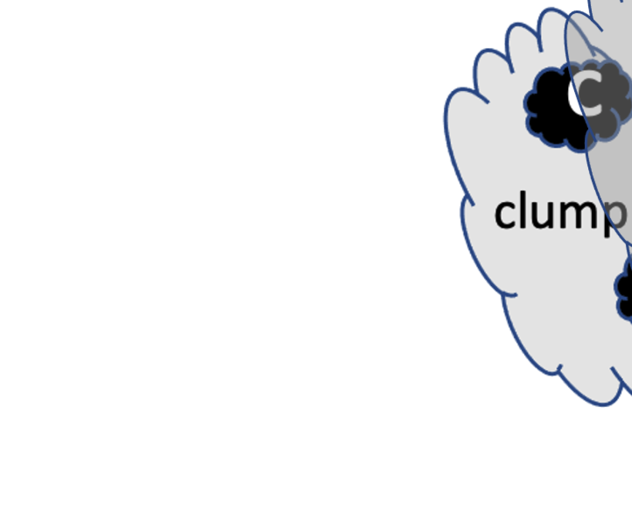
Figure 6: Schematic cartoon showing the possible position of the extinction structures that have been dissipated. Shell ”4” corresponds to the extinction structure that disappeared in the 1940s; clump ”3” to the 1990s excitation jump. The cloud ”2” represents the clump that was associated with the disappearance of narrow absorption lines around 1918 (occulter’s halo). The knot ”1” is the occulter core, which started dissipating around the 2000s. Distances are not to scale, but the angle between our LOS to the central system and the LOS of the Weigelt clumps is 37 degrees (Teodoro et al., 2020).

4.1 Extinction changes around the Weigelt clumps

To deal with the extinction changes, we start by evaluating the extinction in our LOS to the Wegelt clumps by examining the flux increase in the [Fe ii] $\lambda 4641$ line, since this spectral line emission is in the nebular regime, as discussed in Teodoro et al. (2020), and is almost insensitive to changes due to illumination effects by the central system. This is well demonstrated by the steadiness of the [Fe ii] $\lambda 4815$ line flux through the orbital cycle - see their Fig. 9. In this approximation, the change in the flux of [Fe ii] $\lambda 4641$ line is due only to the extinction decrease to our LOS. The extinction in the time interval 1986.22-2002.5 should have decreased by $\Delta\,A_{V}$ $\sim$ 0.3 (see Table 3 in Appendix). This translates into an extinction decrease rate of $\sim$ 0.018 mag.yr^-1. The [Fe iii] $\lambda 4659$ line flux suffers from the same extinction decrease so that the increase of ratio [Fe iii] $\lambda 4659$ /  [Fe ii] $\lambda 4641$ of $\sim$ 22% in this period is due to increased exposure of the Weiglts clumps to the ionizing flux of the secondary star. This occurs if the extinction between the Weigelt clumps and the central binary has decreased.

To evaluate the amount of the extinction decrease between the Weigelt clumps and the central system that caused the ionization ratio increase in 1986.22–2002.5 period we can use rough approximations. As before, we assume the high-density nebular regime in which the [Fe ii] $\lambda 4641$ line flux is constant and so the increase in the ionization ratio is totally due to the increase in the [Fe iii] $\lambda 4659$ line flux increase. Since this is a small increase, we assume that the increase in the ionizing flux incoming from the secondary star was of the same order. So, the decrease in extreme UV extinction is $\sim$ 0.21. If we adopt the reddening law used by Hillier et al. (2001), which is a combination of R $\sim$ 4.2 with a gray component, in the extreme UV (555Å ) the extinction relations is A_UV $/$ A_V $=$ 1.8. This implies in A_V $=$ 0.12. The exact amount of extinction decrease is difficult to assess, primarily because very close to the central system, dust grains are destroyed, and only very large grains remain for a longer time, requiring a combination of reddening laws. This changes with the distance to the star. A full model is out of the scope of this paper.

For the time interval, 2002.5–2019.05 the extinction decrease of our LOS to Weigelt clumps was $\Delta\,A_{V}$ $\sim$ 0.4, which led to an extinction decrease rate of $\sim$ 0.024 mag.yr^-1. In this period, the [Fe iii] $\lambda 4659$ $/$ [Fe ii] $\lambda 4641$ ratio increased by just $\sim$ 10%, which indicates a very small extinction decrease in the LOS of the Weigelt clumps to the central binary (see the flat behavior of this line ratio in Fig. 5).

Just for comparison, using the magnitude brightening of the stellar core (following the method of Damineli et al. 2019), we found that the extinction caused by the ”occulter” (clumps ”1” $+$ ”2”) in our LOS to the central system decreased by $\Delta\,A_{V}$ $\sim$ 1.8 in the time interval 2002.5–2019.05 resulting in a rate of $\sim$ 0.11mag.yr^-1 to our LOS to the central star, which is about $\sim$ 4.6 x faster than in our LOS to the Weigelt clumps.

We further assume that these three recent events: a) the Weigelt clumps excitation increase in early 1990 (this work and Humphreys et al. 2008), b) the start of the occulter’s dissipation around 2000 (Davidson et al., 1999; Martin et al., 2006; Damineli et al., 2019), and c) the disappearance of the UV narrow absorption lines just before 2018 (Gull et al., 2023) are due to a common cause originated in the central system. Using the dates stated above and the distances in Figure 6 the perturbation started in 1980 and traveled at a speed of $\sim$ 400 km s^-1. This is very close to the observed terminal wind speed of the primary star (Groh et al., 2012). Could an outburst in the primary star cause those mentioned above three recent events? We searched for a signal of wind variation using the H$\Delta\,$ line profile. Figure 3 of Damineli et al. 2021 indicates no change since 1992.5 for phase-locked observations ($\phi$ $=$ 0.02). We used one spectrum taken at the OPD observatory in 1998/May/13 ($\phi$ $=$ 9.07) to compare with the one published by Zanella et al. (1984) (1981/Dec/25, $\phi$ $=$ 7.11). They show very similar line profiles, with no indication of a difference in the terminal speed. In addition, there is also no indication of exceptional photometric behavior in the whole object light curve in the period 1980–2000s. This indicates that the primary’s wind has not changed appreciably throughout the last 40 years and the three events we are describing were not caused by a mass ejection of the primary star.

The fact that a) the three dusty clumps we described are located in the broad direction of the binary’s major axis, which coincides with the wind-wind collision cavity orientation for most of the orbit; b) the cause of the changes in the excitation of the clumps traveled at the primary’s wind terminal speed; c) the homunculus brightness over the last three decades remained constant; d) the global properties of the primary’s wind have not changed over the last 40 years; suggesting that the described three events are ”beamed”, not involving a global change in the primary star. We did not identify any mass ejection episode since 1980 that could have triggered these events. It looks as though it has been a silent cumulative work of the primary’s wind blowing inside the wind-wind collision cavity and cleaning out the dust.

5 Data Availability

The complete version of Table 4 is available in the online journal in a machine-readable format following the CDS/Vizier standards.

6 Acknowledgments

AD thanks to CNPq (301490/2019-8) and FAPESP (2011/51680-6) for their support. NDR is grateful for support from the Cottrell Scholar Award #CS-CSA-2023-143 sponsored by the Research Corporation for Science Advancement, as well as support from STScI’s HST GO programs 15611 and 15992. The work of FN is supported by NOIRLab, which is managed by the Association of Universities for Research in Astronomy (AURA) under a cooperative agreement with the National Science Foundation. AFJM is grateful for financial aid from NSERC (Canada).

Based on observations collected at the European Southern Observatory, Chile under Prog-IDs: UVES: 60.A-9022(A), 70.D-0607(A), 71.D-0168(A), 072.D-0524(A), 074.D-0141(A), 077.D-0618(A), 380.D-0036(A), 381.D-0004(A),282.D-5073(A, B, C, D, E), 089.D-0024(A), 592.D-0047(A, B, C). The first three programmes were described in Stahl et al. (2005) and the others in Mehner et al. (2015); FEROS (partial list): 00.A-0000(A), 69.D-0378(A),, 69.D-0381(A), 71.D-0554(A),079.D-0564(C), 079.A-9201(A), 081.D-2008(A), 082.A-9208(A), 082.A-9209(A), 082.A-9210(A), 083.D-0589(A), 086.D-0997(A), 087.D-0946(A),089.D-0975(A), 098.A-9007(A). Spectra can be downloaded from the ESO database by using the instrument name (UVES or FEROS) plus the Julian Date provided in the Appendix Tables. Based on observations made at the Coudé focus of the 1.6-m telescope for the Observatório do Pico dos Dias/LNA (Brazil). Based in part on data from Mt. John University Observatory: MJUO -University of Canterbury - New Zealand). Based in part on observations obtained through NOIRLab (formerly NOAO) allocations of NOAO-09B-153, NOAO-12A-216, NOAO-12B-194, NOAO-13B-328, NOAO-15A-0109, NOAO-18A-0295, NOAO-19B204, NOIRLab-20A-0054, and NOIRLab-21B-0334. This research has used data from the CTIO/SMARTS 1.5m telescope, which is operated as part of the SMARTS Consortium by RecONS (www.recons.org) members Todd Henry, Hodari James, Wei-Chun Jao, and Leonardo Paredes. At the telescope, observations were carried out by Roberto Aviles and Rodrigo.

Appendix A EXTINCTION IN FRONT AND BEHIND CLUMPS ”1” $+$ ”2”, AND ”3”

To evaluate how much the extinction should have decreased in front of the clump ”3” to our LOS, let us compare the evolution of the [Fe ii] $\lambda 4641$ line flux (see Table 3). We use the V$-$band magnitudes of the whole object (columns 2 and 3 or 3 and 5) - first row - to measure the magnitude difference in the stellar continuum between a pair of dates. Then we transform the magnitude difference to a flux ratio of the continuum and multiply it by the line intensity ratio (I $/$ Ic) - second row - to derive the line intensity flux ratio (F $/$ Fc). We calculate the magnitude difference corresponding to the flux ratio of the line for that pair of dates. We assume that there is no intrinsic evolution of the emission in the [Fe ii] $\lambda 4641$ line so the magnitude difference is the extinction difference - columns 4 and 6. The extinction increased by $\Delta\,A_{V}$ $=$ 0.28 mag in the time interval 1986.22–2002.5 and $\Delta\,A_{V}$ $=$ 0.40 mag in the time interval 2002.5–2019.05. These values are for the extinction decrease in front of clump ”3” to our LOS and are due to dissipation within the Homunculus.

For the stellar core, we can measure the extinction difference of the dissipating occulter ”1” $+$ ”2”) (see in Figure 6) for the dates 2002.5–2019.05. We follow the procedure described by Damineli et al. (2019), which is to start from the V$-$band magnitude of the whole object at one of the dates and subtract the flux of the Homunculus nebula, which is approximately constant (V_H $\sim$ 5.5) - Davidson et al. (1995) gives 5.7. We repeat the same calculation for the second date and translate the brightness increase into an extinction decrease to our LOS towards the central star. For the pair of dates 2002.5 and 2019.05 we obtain an extinction decrease $\Delta\,A_{V}$ $=$ 1.8 mag, which is $\sim$ 4.6 x higher than that of the Weigelt clumps LOS to the central star in the same period. This extinction decrease adds the changes inside the clumps ”1” $+$ ”2” to that within the Homunculus.

Table 3: Extinction decrease in our LOS to the Weigelt clumps and to the central star

	1986.22	2002.5	1986–2002	2019.05	2002–19
Parameter	Year	Year	$\Delta\,A_{V}$ mag	Year	$\Delta\,A_{V}$ mag
Vwhole	5.87	5.15	-	4.31	-
I/Ic[FeII] 4641∗∗	2.4	2.14	0.28	1.43	0.4
Vcore∗	-	6.55	-	4.76	1.8

Notes: (*) - Magnitudes of the core are obtained following Damineli et al. (2019) - see text.
(**) - After degrading spectral resolution to R $=$ 5 000

It is possible to evaluate the total extinction of the occulter (clumps ”1” $+$ ”2” ) by using the extinction in front of the Weigelt BCD knots reported by Davidson et al. (1995) - $A_{V}$ $\sim$ 2.0 - using data taken with HST in 1991.4. By subtracting the total extinction decrease from that date to 2019.5, the total extinction (interstellar plus within the Homunmculus) in our LOS to the Weigelt clumps should have been $A_{V}$ $\sim$ 1.44. For the measured stellar core brightness, V $=$ 4.76 - see Table  3 - the brightness after correcting for the same material that affects the Weigelt clumps (Homunculus plus interstellar) would be V $=$ 3.32. Using the unreddened apparent magnitude from Hillier et al. (2001) model, V₀ $=$ 0.94, the extinction caused by the occulter to our LOS should have been $A_{V}$ $\sim$ 2.38 in 2019.5. The extinction decrease since 1991.4, reported by Davidson et al. (1995) - $A_{V}$ $\sim$ 6.1 - should have been $\Delta\,A_{V}$ $\sim$ 3.88 which translates into an average rate of 0.14 mag.yr^-1, in good agreement with the brightening rate (0.13 mag.yr^-1) reported by Damineli et al. (2019) for the period 1998.2–2015.7. At this rate, the dissipation of the occulter (no more extinction decrease) would be completed in 2040.

Appendix B Extended data tables (online material)

Table 4: Normalized line intensities.

row	Observat	JD	year	phase	FeII	[FeII]	[FeIII]	Vflux
				(14$=$2020.2)	(4631$\AA$)	(4641$\AA$)	(4659$\AA$)	(norm)
1	ESO/FEROS	2448793.99	1992.4675	9.00514	3.14	2.79	1.33	0.71
2	ESO/FEROS	2448825.01	1992.5524	9.02047	3.01	2.48	1.15	0.71
3	ESO/FEROS	2448830.02	1992.5661	9.02295	3.21	2.55	1.27	0.71
4	ESO/FEROS	2448839.00	1992.5907	9.02739	3.35	2.52	1.25	0.71
5	ESO/FEROS	2448843.99	1992.6043	9.02986	3.23	2.32	1.18	0.71
6	ESO/FEROS	2449063.11	1993.2043	9.13819	7.05	3.52	3.10	0.65
7	ESO/FEROS	2449068.11	1993.2180	9.14066	7.06	3.58	3.11	0.65
8	ESO/FEROS	2449073.15	1993.2318	9.14315	7.16	3.43	3.09	0.65
9	ESO/FEROS	2449078.11	1993.2453	9.14560	6.44	3.22	3.09	0.65
10	ESO/FEROS	2449083.10	1993.2590	9.14807	6.34	3.19	2.96	0.65
11	ESO/FEROS	2449088.11	1993.2727	9.15055	6.21	3.00	2.96	0.65
12	ESO/FEROS	2449095.09	1993.2918	9.15400	6.40	3.00	2.90	0.65
13	ESO/FEROS	2449102.11	1993.3110	9.15747	6.81	3.53	3.32	0.65
14	ESO/FEROS	2449106.11	1993.3220	9.15944	6.94	3.47	3.36	0.65
15	ESO/FEROS	2449110.18	1993.3332	9.16146	6.16	3.24	3.07	0.65
16	ESO/FEROS	2449113.08	1993.3411	9.16289	5.91	3.39	3.00	0.65
17	ESO/FEROS	2449114.18	1993.3441	9.16343	5.62	3.14	5.62	0.65
18	ESO/FEROS	2449128.04	1993.3820	9.17029	6.07	3.07	3.09	0.65
19	ESO/FEROS	2449138.09	1993.4096	9.17526	6.20	3.24	3.13	0.65
20	ESO/FEROS	2449395.37	1994.1139	9.30245	6.63	3.41	3.43	0.66
21	ESO/FEROS	2449408.03	1994.1486	9.30871	5.00	2.92	3.50	0.66
22	ESO/FEROS	2449424.02	1994.1924	9.31662	4.94	2.62	3.45	0.66
23	ESO/FEROS	2449448.10	1994.2583	9.32852	4.93	2.62	3.58	0.66
24	ESO/FEROS	2449467.06	1994.3102	9.33790	5.00	2.69	3.50	0.66
25	ESO/FEROS	2449472.10	1994.3240	9.34039	4.44	2.54	3.32	0.66
26	ESO/FEROS	2449514.04	1994.4389	9.36112	4.77	2.67	3.47	0.66
27	ESO/FEROS	2449520.11	1994.4555	9.36412	5.16	2.81	3.73	0.66
28	ESO/FEROS	2449522.04	1994.4607	9.36508	5.22	2.79	3.69	0.66
29	ESO/FEROS	2449525.03	1994.4689	9.36655	5.55	2.97	4.03	0.65
30	ESO/FEROS	2449527.03	1994.4744	9.36754	5.15	2.82	3.71	0.65
31	ESO/FEROS	2449532.02	1994.4881	9.37001	4.65	2.59	3.56	0.65
32	ESO/FEROS	2449770.24	1995.1403	9.48778	5.17	2.70	4.78	0.58
33	ESO/FEROS	2449786.12	1995.1838	9.49563	5.52	2.79	4.99	0.58
34	ESO/FEROS	2449800.24	1995.2224	9.50262	5.02	2.68	4.63	0.58
35	ESO/FEROS	2449836.05	1995.3205	9.52032	5.51	2.88	4.94	0.58
36	ESO/FEROS	2449846.04	1995.3478	9.52526	4.87	2.52	4.60	0.58
37	ESO/FEROS	2449860.07	1995.3862	9.53219	5.15	2.81	3.82	0.57
38	ESO/FEROS	2450120.28	1996.0987	9.66084	5.73	3.03	5.78	0.59
39	ESO/FEROS	2450134.27	1996.1370	9.66776	5.60	3.05	5.75	0.59
40	ESO/FEROS	2450146.37	1996.1701	9.67374	5.60	2.99	5.63	0.59
41	ESO/FEROS	2450160.25	1996.2081	9.68060	5.70	3.05	5.70	0.59
42	ESO/FEROS	2450174.26	1996.2464	9.68753	5.89	3.25	5.80	0.59
43	ESO/FEROS	2450188.31	1996.2849	9.69447	6.26	3.28	5.80	0.59
44	ESO/FEROS	2450201.23	1996.3203	9.70086	5.05	3.14	5.75	0.59
45	LNA/OPD	2450211.50	1996.3484	9.70594	1.53	1.20	1.81	0.59
46	LNA/OPD	2450211.50	1996.3484	9.70594	1.70	1.26	1.84	0.59
47	ESO/FEROS	2450237.97	1996.4209	9.71902	5.00	3.01	5.70	0.59
48	ESO/FEROS	2450238.01	1996.4210	9.71905	5.10	3.00	5.78	0.59
49	ESO/FEROS	2450241.95	1996.4318	9.72099	5.20	3.05	5.80	0.59
50	ESO/FEROS	2450242.02	1996.4319	9.72103	5.50	2.94	5.72	0.59
51	ESO/FEROS	2450244.08	1996.4376	9.72205	5.14	2.84	5.25	0.59
52	ESO/FEROS	2450449.25	1996.9993	9.82348	5.29	2.75	5.11	0.62
53	ESO/FEROS	2450450.26	1997.0021	9.82398	5.10	2.90	5.40	0.62
54	ESO/FEROS	2450451.21	1997.0047	9.82445	5.36	3.33	4.90	0.62
55	ESO/FEROS	2450452.21	1997.0074	9.82494	6.08	3.30	4.85	0.62
56	ESO/FEROS	2450453.19	1997.0101	9.82543	6.79	3.37	4.88	0.62
57	ESO/FEROS	2450454.22	1997.0129	9.82594	5.97	3.28	4.76	0.62
58	ESO/FEROS	2450455.30	1997.0159	9.82647	6.49	3.34	4.90	0.62
59	ESO/FEROS	2450456.22	1997.0184	9.82692	6.44	3.30	4.90	0.62
60	ESO/FEROS	2450457.18	1997.0210	9.82740	6.11	3.43	4.79	0.62
61	ESO/FEROS	2450464.34	1997.0406	9.83094	6.14	3.32	4.83	0.62
62	ESO/FEROS	2450472.35	1997.0626	9.83490	6.20	3.28	4.96	0.62
63	ESO/FEROS	2450476.33	1997.0734	9.83686	7.00	3.42	5.00	0.62
64	ESO/FEROS	2450516.18	1997.1826	9.85657	7.10	3.41	5.00	0.62
65	ESO/FEROS	2450518.13	1997.1879	9.85753	6.67	3.48	5.08	0.62
66	ESO/FEROS	2450520.13	1997.1934	9.85852	5.34	3.33	4.20	0.62
67	ESO/FEROS	2450522.19	1997.1990	9.85954	5.30	2.98	3.95	0.62
68	ESO/FEROS	2450524.20	1997.2045	9.86053	5.75	3.13	4.18	0.62
69	ESO/FEROS	2450527.12	1997.2125	9.86198	5.70	3.18	4.18	0.62
70	ESO/FEROS	2450531.14	1997.2235	9.86396	5.65	3.13	4.20	0.62
71	ESO/FEROS	2450533.11	1997.2289	9.86494	5.73	3.16	4.15	0.62
72	ESO/FEROS	2450535.17	1997.2345	9.86596	5.56	3.26	4.15	0.62
73	ESO/FEROS	2450537.15	1997.2400	9.86694	5.76	3.08	4.17	0.62
74	ESO/FEROS	2450539.15	1997.2454	9.86792	5.68	3.16	4.15	0.62
75	ESO/FEROS	2450541.16	1997.2510	9.86892	5.81	3.19	4.13	0.62
76	ESO/FEROS	2450543.16	1997.2564	9.86991	5.90	3.27	4.25	0.62
77	ESO/FEROS	2450545.14	1997.2619	9.87089	5.82	3.19	4.22	0.62
78	ESO/FEROS	2450547.15	1997.2673	9.87188	5.94	3.27	4.21	0.62
79	ESO/FEROS	2450549.15	1997.2728	9.87287	5.76	3.25	4.21	0.62
80	ESO/FEROS	2450551.16	1997.2783	9.87386	5.70	3.20	4.17	0.62
81	ESO/FEROS	2450553.16	1997.2838	9.87485	6.00	3.40	4.45	0.62
82	ESO/FEROS	2450556.08	1997.2918	9.87629	5.93	3.38	4.35	0.62
83	ESO/FEROS	2450557.11	1997.2946	9.87680	5.88	3.13	4.22	0.62
84	ESO/FEROS	2450559.08	1997.3000	9.87778	6.39	3.39	4.51	0.62
85	ESO/FEROS	2450561.08	1997.3055	9.87876	7.28	3.64	4.80	0.62
86	ESO/FEROS	2450563.09	1997.3110	9.87976	6.92	3.54	4.72	0.62
87	ESO/FEROS	2450565.08	1997.3164	9.88074	8.10	3.84	5.20	0.62
88	LNA/OPD	2450652.46	1997.5557	9.92394	1.58	1.20	1.83	0.67
89	LNA/OPD	2450652.50	1997.5558	9.92396	1.56	1.21	1.87	0.67
90	LNA/OPD	2450761.833	1997.8551	9.97802	2.00	1.41	1.95	0.67
91	LNA/OPD	2450762.50	1997.8569	9.97835	1.61	1.20	1.79	0.67
92	LNA/OPD	2450762.79	1997.8577	9.97849	1.57	1.21	1.87	0.67
93	LNA/OPD	2450762.79	1997.8577	9.97849	1.58	1.20	1.76	0.67
94	MSO	2450771.20	1997.8808	9.98265	1.39	1.33	1.02	0.67
95	MSO	2450797.14	1997.9518	9.99547	1.40	1.31	1.02	0.77
96	MSO	2450808.12	1997.9818	10.00090	1.36	1.29	1.01	0.77
97	MSO	2450870.10	1998.1515	10.03154	1.39	1.32	1.01	0.77
98	MSO	2450884.00	1998.1896	10.03841	1.34	1.29	1.01	0.77
99	MSO	2450896.04	1998.2226	10.04437	1.42	1.32	1.02	0.77
100	LNA/OPD	2450946.46	1998.3606	10.06929	1.61	1.21	1.84	0.77
101	LNA/OPD	2450946.50	1998.3607	10.06931	1.47	1.20	1.72	0.71
102	ESO/FEROS	2451173.23	1998.9815	10.18140	7.64	3.77	5.13	0.84
103	MSO	2451188.10	1999.0222	10.18876	1.55	1.40	1.10	0.84
104	ESO/FEROS	2451381.98	1999.5530	10.28461	7.38	3.54	4.70	0.84
105	ESO/FEROS	2451391.97	1999.5803	10.28955	4.57	2.55	3.10	0.98
106	ESO/FEROS	2451594.41	2000.1346	10.38963	1.97	1.48	1.43	0.98
107	ESO/FEROS	2451654.05	2000.2979	10.41912	2.00	1.57	1.49	0.98
108	ESO/FEROS	2452010.97	2001.2751	10.59557	2.09	1.59	1.40	0.98
109	ESO/FEROS	2452301.19	2002.0697	10.73906	2.15	1.57	1.32	1.00
110	LNA/OPD	2452460.375	2002.5055	10.81776	2.50	1.54	2.05	1.00
111	ESO/UVES	2452615.32	2002.9297	10.89436	1.59	1.23	1.88	1.00
112	ESO/UVES	2452620.34	2002.9434	10.89684	1.49	1.15	1.77	1.00
113	ESO/UVES	2452684.13	2003.1181	10.92838	1.52	1.15	1.74	0.96
114	LNA/OPD	2452773.54	2003.3629	10.97258	1.85	1.37	1.96	0.96
115	ESO/UVES	2452793.98	2003.4188	10.98269	1.59	1.20	1.87	0.96
116	LNA/OPD	2452810.52	2003.4641	10.99086	1.95	1.45	1.33	0.96
117	LNA/OPD	2452811.52	2003.4669	10.99136	1.95	1.49	1.36	0.96
118	LNA/OPD	2452812.52	2003.4696	10.99185	1.96	1.44	1.48	0.96
119	LNA/OPD	2452813.52	2003.4723	10.99235	1.94	1.44	1.52	0.96
120	LNA/OPD	2452814.52	2003.4751	10.99284	1.95	1.44	1.67	0.96
121	LNA/OPD	2452814.52	2003.4751	10.99284	1.83	1.34	1.70	0.96
122	LNA/OPD	2452815.52	2003.4778	10.99334	1.87	1.35	1.72	0.96
123	LNA/OPD	2452815.52	2003.4778	10.99334	2.02	1.45	2.07	0.96
124	LNA/OPD	2452816.52	2003.4805	10.99383	2.02	1.46	2.07	0.96
125	LNA/OPD	2452817.52	2003.4833	10.99432	1.97	1.47	2.07	0.96
126	LNA/OPD	2452819.52	2003.4888	10.99531	1.94	1.42	2.04	0.96
127	LNA/OPD	2452820.52	2003.4915	10.99581	1.92	1.37	2.01	0.96
128	LNA/OPD	2452822.06	2003.4957	10.99657	1.44	1.33	1.02	0.96
129	LNA/OPD	2452822.38	2003.4966	10.99672	2.14	1.51	1.85	0.96
130	LNA/OPD	2452822.41	2003.4967	10.99674	1.48	1.32	1.02	0.96
131	LNA/OPD	2452823.375	2003.4993	10.99722	2.29	1.57	1.90	0.96
132	LNA/OPD	2452823.77	2003.5004	10.99741	1.45	1.27	1.01	0.96
133	LNA/OPD	2452823.77	2003.5004	10.99741	1.58	1.36	1.00	0.96
134	LNA/OPD	2452824.375	2003.5021	10.99771	2.45	1.60	2.13	0.96
135	ESO/UVES	2452825.01	2003.5038	10.99803	1.58	1.23	1.90	0.96
136	LNA/OPD	2452825.97	2003.5064	10.99850	1.69	1.31	1.00	0.96
137	LNA/OPD	2452826.375	2003.5075	10.99870	2.22	1.51	2.03	0.96
138	LNA/OPD	2452826.375	2003.5075	10.99870	2.20	1.61	2.10	0.96
139	LNA/OPD	2452827.375	2003.5103	10.99920	2.16	1.55	1.64	0.96
140	LNA/OPD	2452827.98	2003.5119	10.99950	1.58	1.30	0.98	0.96
141	LNA/OPD	2452828.38	2003.5130	10.99969	2.06	1.51	1.56	0.96
142	LNA/OPD	2452829.98	2003.5174	11.00048	1.57	1.28	0.98	0.96
143	LNA/OPD	2452830.38	2003.5185	11.00068	1.97	1.43	1.42	1.15
144	LNA/OPD	2452840.98	2003.5475	11.00592	1.58	1.29	1.01	1.15
145	LNA/OPD	2452987.71	2003.9492	11.07846	1.45	1.31	1.02	1.15
146	LNA/OPD	2452987.833	2003.9496	11.07853	2.40	1.70	2.06	1.15
147	ESO/UVES	2453413.39	2005.1147	11.28891	1.50	1.15	1.80	1.25
148	ESO/UVES	2453834.11	2006.2666	11.49692	1.47	1.18	1.82	1.51
149	ESO/UVES	2454475.27	2008.0220	11.81390	1.45	1.17	1.75	1.17
150	ESO/UVES	2454513.30	2008.1261	11.83270	1.59	1.24	1.91	1.17
151	ESO/UVES	2454535.28	2008.1863	11.84357	1.54	1.21	1.80	1.17
152	ESO/UVES	2454554.28	2008.2383	11.85296	1.61	1.20	1.97	1.17
153	ESO/UVES	2454567.01	2008.2731	11.85925	1.53	1.24	1.90	1.17
154	ESO/UVES	2454583.02	2008.3170	11.86717	1.67	1.27	2.00	1.17
155	LNA/OPD	2454596.417	2008.3536	11.87379	2.41	1.48	2.05	1.17
156	LNA/OPD	2454596.50	2008.3539	11.87383	1.90	1.45	2.07	1.17
157	LNA/OPD	2454598.40	2008.3591	11.87477	1.83	1.37	1.97	1.17
158	ESO/FEROS	2454601.02	2008.3663	11.87607	1.85	1.44	1.14	1.17
159	ESO/UVES	2454629.02	2008.4429	11.88991	1.70	1.22	2.05	1.17
160	ESO/UVES	2454656.03	2008.5169	11.90326	1.68	1.31	2.14	1.19
161	ESO/FEROS	2454821.33	2008.9694	11.98499	1.78	1.42	1.09	1.36
162	ESO/FEROS	2454822.37	2008.9723	11.98550	1.90	1.45	1.37	1.36
163	ESO/FEROS	2454823.29	2008.9748	11.98596	1.64	1.37	1.05	1.36
164	ESO/FEROS	2454824.31	2008.9776	11.98646	1.72	1.42	1.05	1.36
165	ESO/FEROS	2454825.30	2008.9803	11.98695	1.62	1.39	1.05	1.36
166	ESO/FEROS	2454827.37	2008.9859	11.98797	1.59	1.33	1.03	1.36
167	ESO/FEROS	2454828.36	2008.9887	11.98846	1.45	1.35	1.02	1.36
168	ESO/FEROS	2454829.37	2008.9914	11.98896	1.80	1.40	1.11	1.36
169	ESO/FEROS	2454830.37	2008.9942	11.98946	1.65	1.47	1.04	1.36
170	ESO/FEROS	2454831.37	2008.9969	11.98995	1.56	1.37	1.02	1.36
171	ESO/FEROS	2454832.37	2008.9996	11.99044	1.60	1.44	1.08	1.36
172	ESO/FEROS	2454833.37	2009.0024	11.99094	1.52	1.36	1.02	1.36
173	ESO/FEROS	2454834.38	2009.0051	11.99144	1.55	1.35	1.48	1.36
174	ESO/Hexapod	2454844.36	2009.0325	11.99637	2.24	1.49	2.14	1.36
175	ESO/Hexapod	2454845.36	2009.0352	11.99686	2.02	1.42	1.96	1.36
176	LNA/OPD	2454882.63	2009.1372	12.01529	1.85	1.39	2.07	1.36
177	ESO/Hexapod	2454897.50	2009.1780	12.02264	2.33	1.57	2.13	1.36
178	LNA/OPD	2454940.48	2009.2956	12.04389	1.87	1.39	2.06	1.36
179	ESO/FEROS	2454953.10	2009.3302	12.05013	1.48	1.31	1.01	1.36
180	ESO/FEROS	2454955.08	2009.3356	12.05111	1.40	1.31	1.02	1.44
181	CTIO/CHIRON	2455989.69	2012.1682	12.56261	2.49	1.58	2.37	1.44
182	CTIO/CHIRON	2455993.75	2012.1793	12.56462	2.54	1.63	2.45	1.44
183	CTIO/CHIRON	2456001.73	2012.2012	12.56856	2.47	1.57	2.33	1.44
184	CTIO/CHIRON	2456013.69	2012.2339	12.57447	2.65	1.65	2.52	1.44
185	CTIO/CHIRON	2456221.89	2012.8039	12.67741	2.48	1.56	2.30	1.44
186	CTIO/CHIRON	2456236.84	2012.8449	12.68480	2.70	1.55	2.40	1.44
187	CTIO/CHIRON	2456238.87	2012.8504	12.68580	2.71	1.66	2.49	1.44
188	CTIO/CHIRON	2456248.81	2012.8777	12.69072	2.55	1.63	2.32	1.44
189	CTIO/CHIRON	2456254.88	2012.8943	12.69372	2.80	1.64	2.50	1.44
190	CTIO/CHIRON	2456260.78	2012.9104	12.69663	2.80	1.64	2.50	1.73
191	CTIO/CHIRON	2456275.82	2012.9516	12.70407	2.70	1.64	2.44	1.73
192	CTIO/CHIRON	2456289.80	2012.9899	12.71098	2.82	1.63	2.50	1.73
193	CTIO/CHIRON	2456361.65	2013.1866	12.74650	2.67	1.63	2.39	1.73
194	CTIO/CHIRON	2456401.59	2013.2959	12.76625	2.82	1.77	2.67	1.73
195	CTIO/CHIRON	2456417.59	2013.3397	12.77416	2.65	1.63	2.31	1.62
196	CTIO/CHIRON	2456607.84	2013.8606	12.86822	2.86	1.58	2.40	1.58
197	CTIO/CHIRON	2456612.87	2013.8744	12.87070	2.80	1.66	2.52	1.58
198	CTIO/CHIRON	2456656.70	2013.9944	12.89237	2.80	1.66	2.48	1.64
199	CTIO/CHIRON	2456659.71	2014.0026	12.89386	2.81	1.71	2.56	1.64
200	CTIO/CHIRON	2456664.67	2014.0162	12.89631	2.83	1.79	2.66	1.64
201	CTIO/CHIRON	2456670.78	2014.0329	12.89933	2.78	1.69	2.35	1.64
202	CTIO/CHIRON	2456672.84	2014.0386	12.90035	2.82	1.77	2.60	1.64
203	CTIO/CHIRON	2456677.76	2014.0520	12.90278	2.83	1.73	2.53	1.64
204	CTIO/CHIRON	2456687.71	2014.0793	12.90770	2.85	1.79	2.55	1.64
205	CTIO/CHIRON	2456690.69	2014.0875	12.90918	2.85	1.79	2.62	1.64
206	CTIO/CHIRON	2456697.73	2014.1067	12.91265	2.83	1.74	2.53	1.64
207	CTIO/CHIRON	2456710.67	2014.1421	12.91905	2.80	1.69	2.37	1.64
208	CTIO/CHIRON	2456712.69	2014.1477	12.92005	2.81	1.77	2.50	1.64
209	CTIO/CHIRON	2456718.71	2014.1642	12.92303	2.80	1.73	2.40	1.64
210	CTIO/CHIRON	2456725.57	2014.1829	12.92642	2.90	1.82	2.51	1.64
211	CTIO/CHIRON	2456729.56	2014.1939	12.92839	2.81	1.77	2.44	1.64
212	CTIO/CHIRON	2456732.61	2014.2022	12.92990	2.95	1.76	2.47	1.64
213	CTIO/CHIRON	2456739.55	2014.2212	12.93333	2.92	1.74	2.29	1.64
214	CTIO/CHIRON	2456746.52	2014.2403	12.93678	2.90	1.82	2.40	1.64
215	CTIO/CHIRON	2456750.54	2014.2513	12.93877	2.90	1.80	2.30	1.64
216	CTIO/CHIRON	2456754.55	2014.2623	12.94075	2.88	1.80	2.23	1.64
217	CTIO/CHIRON	2456765.59	2014.2925	12.94621	2.94	1.83	2.20	1.64
218	CTIO/CHIRON	2456766.55	2014.2951	12.94668	2.82	1.78	2.13	1.64
219	CTIO/CHIRON	2456767.51	2014.2978	12.94716	2.76	1.78	2.02	1.64
220	CTIO/CHIRON	2456774.55	2014.3170	12.95063	2.73	1.77	1.98	1.64
221	CTIO/CHIRON	2456781.47	2014.3360	12.95406	2.69	1.74	1.95	1.64
222	CTIO/CHIRON	2456791.55	2014.3636	12.95904	2.57	1.71	1.55	1.76
223	CTIO/CHIRON	2456795.51	2014.3744	12.96100	2.49	1.70	1.39	1.76
224	CTIO/CHIRON	2456800.46	2014.3880	12.96345	2.34	1.69	1.21	1.76
225	CTIO/CHIRON	2456801.50	2014.3908	12.96396	2.23	1.65	1.15	1.76
226	CTIO/CHIRON	2456803.53	2014.3964	12.96496	1.99	1.63	1.09	1.76
227	CTIO/CHIRON	2456810.48	2014.4154	12.96840	1.98	1.61	1.09	1.76
228	CTIO/CHIRON	2456818.51	2014.4374	12.97237	1.93	1.58	1.08	1.76
229	CTIO/CHIRON	2456819.53	2014.4402	12.97287	1.89	1.59	1.08	1.76
230	CTIO/CHIRON	2456823.54	2014.4512	12.97486	1.90	1.60	1.08	1.95
231	CTIO/CHIRON	2456824.52	2014.4538	12.97534	1.84	1.58	1.09	1.95
232	CTIO/CHIRON	2456829.50	2014.4675	12.97780	1.83	1.55	1.08	1.95
233	CTIO/CHIRON	2456832.50	2014.4757	12.97929	1.73	1.57	1.10	1.95
234	CTIO/CHIRON	2456835.53	2014.4840	12.98079	1.75	1.56	1.10	1.95
235	CTIO/CHIRON	2456836.50	2014.4866	12.98126	1.75	1.54	1.08	1.95
236	CTIO/CHIRON	2456845.46	2014.5112	12.98569	1.74	1.57	1.09	1.95
237	CTIO/CHIRON	2456850.51	2014.5250	12.98819	2.20	1.57	1.07	1.95
238	CTIO/CHIRON	2456855.46	2014.5386	12.99064	2.15	1.54	1.20	1.95
239	CTIO/CHIRON	2456857.45	2014.5440	12.99162	2.29	1.57	1.23	1.95
240	CTIO/CHIRON	2456858.45	2014.5468	12.99212	2.30	1.62	1.24	1.95
241	CTIO/CHIRON	2456859.47	2014.5495	12.99262	2.30	1.56	1.22	1.95
242	CTIO/CHIRON	2456863.47	2014.5605	12.99459	2.32	1.57	1.25	1.91
243	CTIO/CHIRON	2456864.47	2014.5632	12.99509	2.36	1.59	1.23	1.91
244	CTIO/CHIRON	2456866.51	2014.5688	12.99610	2.30	1.58	1.27	1.91
245	CTIO/CHIRON	2456867.46	2014.5714	12.99657	2.35	1.59	1.29	1.91
246	CTIO/CHIRON	2456870.46	2014.5796	12.99805	2.27	1.58	1.26	1.91
247	CTIO/CHIRON	2456871.46	2014.5824	12.99855	2.31	1.59	1.28	1.91
248	CTIO/CHIRON	2456872.46	2014.5851	12.99904	2.37	1.61	1.32	1.91
249	CTIO/CHIRON	2456873.46	2014.5879	12.99954	2.39	1.62	1.34	1.91
250	CTIO/CHIRON	2456874.45	2014.5906	13.00003	2.34	1.63	1.37	1.91
251	CTIO/CHIRON	2456878.48	2014.6016	13.00202	2.37	1.58	1.35	1.91
252	CTIO/CHIRON	2456879.47	2014.6043	13.00250	2.35	1.60	1.38	1.91
253	CTIO/CHIRON	2456882.46	2014.6125	13.00399	2.33	1.55	1.36	1.91
254	CTIO/CHIRON	2456883.46	2014.6152	13.00448	2.23	1.52	1.37	1.91
255	CTIO/CHIRON	2456885.46	2014.6207	13.00547	2.31	1.56	1.41	1.91
256	CTIO/CHIRON	2456886.47	2014.6235	13.00597	2.31	1.55	1.43	1.91
257	CTIO/CHIRON	2456943.90	2014.7807	13.03436	2.36	1.59	1.48	1.78
258	CTIO/CHIRON	2456944.90	2014.7834	13.03485	2.34	1.59	1.46	1.78
259	CTIO/CHIRON	2456950.88	2014.7998	13.03781	2.27	1.54	1.45	1.78
260	CTIO/CHIRON	2456951.87	2014.8025	13.03830	2.33	1.57	1.48	1.78
261	CTIO/CHIRON	2456952.86	2014.8052	13.03879	2.26	1.53	1.47	1.78
262	CTIO/CHIRON	2456953.88	2014.8080	13.03929	2.26	1.52	1.49	1.78
263	CTIO/CHIRON	2456954.83	2014.8106	13.03976	2.31	1.56	1.49	1.78
264	CTIO/CHIRON	2456955.86	2014.8134	13.04027	2.36	1.59	1.54	1.78
265	CTIO/CHIRON	2456956.87	2014.8162	13.04077	2.34	1.59	1.52	1.78
266	CTIO/CHIRON	2456957.89	2014.8190	13.04128	2.33	1.55	1.53	1.78
267	CTIO/CHIRON	2456958.86	2014.8217	13.04176	2.27	1.53	1.56	1.78
268	CTIO/CHIRON	2456959.85	2014.8244	13.04224	2.26	1.53	1.56	1.78
269	CTIO/CHIRON	2456961.85	2014.8298	13.04323	2.29	1.54	1.54	1.78
270	CTIO/CHIRON	2456964.87	2014.8381	13.04472	2.34	1.54	1.62	1.78
271	CTIO/CHIRON	2456965.86	2014.8408	13.04522	2.30	1.54	1.60	1.78
272	CTIO/CHIRON	2456968.87	2014.8491	13.04670	2.30	1.53	1.61	1.78
273	CTIO/CHIRON	2456969.86	2014.8518	13.04720	2.27	1.53	1.59	1.78
274	CTIO/CHIRON	2456972.88	2014.8600	13.04869	2.31	1.55	1.65	1.78
275	CTIO/CHIRON	2456974.85	2014.8654	13.04966	2.29	1.55	1.62	1.78
276	CTIO/CHIRON	2456977.85	2014.8736	13.05114	2.23	1.53	1.61	1.78
277	CTIO/CHIRON	2456979.84	2014.8791	13.05213	2.25	1.52	1.63	1.78
278	CTIO/CHIRON	2456980.81	2014.8817	13.05261	2.30	1.54	1.66	1.78
279	CTIO/CHIRON	2456982.81	2014.8872	13.05360	2.23	1.54	1.65	1.78
280	CTIO/CHIRON	2456984.82	2014.8927	13.05459	2.29	1.58	1.69	1.78
281	CTIO/CHIRON	2456985.83	2014.8955	13.05509	2.18	1.54	1.64	1.78
282	CTIO/CHIRON	2456986.87	2014.8983	13.05560	2.25	1.51	1.67	1.78
283	CTIO/CHIRON	2456988.79	2014.9036	13.05656	2.16	1.55	1.70	1.78
284	CTIO/CHIRON	2456990.76	2014.9090	13.05753	2.23	1.54	1.73	1.78
285	CTIO/CHIRON	2456992.78	2014.9145	13.05853	2.22	1.51	1.70	1.78
286	CTIO/CHIRON	2456994.82	2014.9201	13.05953	2.26	1.49	1.70	1.78
287	CTIO/CHIRON	2456996.85	2014.9257	13.06054	2.25	1.56	1.74	1.78
288	CTIO/CHIRON	2456998.81	2014.9310	13.06150	2.21	1.52	1.70	1.78
289	CTIO/CHIRON	2457000.84	2014.9366	13.06251	2.23	1.52	1.73	1.78
290	CTIO/CHIRON	2457007.85	2014.9558	13.06598	2.23	1.52	1.71	1.83
291	CTIO/CHIRON	2457008.74	2014.9582	13.06642	2.25	1.54	1.75	1.83
292	CTIO/CHIRON	2457009.75	2014.9610	13.06691	2.16	1.47	1.68	1.83
293	CTIO/CHIRON	2457012.82	2014.9694	13.06843	2.25	1.54	1.74	1.83
294	CTIO/CHIRON	2457013.81	2014.9721	13.06892	2.22	1.54	1.78	1.83
295	CTIO/CHIRON	2457014.74	2014.9746	13.06938	2.28	1.53	1.80	1.83
296	CTIO/CHIRON	2457015.77	2014.9775	13.06989	2.19	1.51	1.77	1.83
297	CTIO/CHIRON	2457016.80	2014.9803	13.07040	2.09	1.46	1.73	1.83
298	CTIO/CHIRON	2457018.78	2014.9857	13.07138	2.23	1.52	1.84	1.83
299	CTIO/CHIRON	2457021.84	2014.9941	13.07289	2.14	1.45	1.77	1.83
300	CTIO/CHIRON	2457022.75	2014.9966	13.07334	2.15	1.51	1.77	1.83
301	CTIO/CHIRON	2457025.83	2015.0050	13.07486	2.12	1.48	1.77	1.83
302	CTIO/CHIRON	2457026.70	2015.0074	13.07530	2.11	1.49	1.72	1.83
303	CTIO/CHIRON	2457030.69	2015.0183	13.07727	2.06	1.45	1.71	1.83
304	CTIO/CHIRON	2457032.82	2015.0241	13.07832	2.27	1.56	1.91	1.83
305	CTIO/CHIRON	2457035.72	2015.0321	13.07976	2.15	1.51	1.80	1.83
306	CTIO/CHIRON	2457037.82	2015.0378	13.08079	2.25	1.54	1.95	1.83
307	CTIO/CHIRON	2457038.85	2015.0407	13.08130	2.04	1.42	1.74	1.83
308	CTIO/CHIRON	2457039.83	2015.0434	13.08179	2.06	1.45	1.81	1.83
309	CTIO/CHIRON	2457040.71	2015.0458	13.08222	2.07	1.45	1.83	1.83
310	CTIO/CHIRON	2457043.85	2015.0543	13.08377	2.15	1.50	1.87	1.83
311	CTIO/CHIRON	2457046.68	2015.0621	13.08518	2.14	1.51	1.90	1.83
312	CTIO/CHIRON	2457047.69	2015.0648	13.08567	2.18	1.49	1.92	1.83
313	CTIO/CHIRON	2457048.81	2015.0679	13.08623	2.20	1.49	1.92	1.83
314	CTIO/CHIRON	2457050.73	2015.0732	13.08718	2.08	1.45	1.84	1.83
315	CTIO/CHIRON	2457051.85	2015.0762	13.08773	2.20	1.50	1.94	1.83
316	CTIO/CHIRON	2457059.79	2015.0980	13.09165	2.16	1.51	1.94	1.83
317	CTIO/CHIRON	2457060.66	2015.1004	13.09209	2.14	1.49	1.91	1.83
318	CTIO/CHIRON	2457061.85	2015.1036	13.09267	2.09	1.45	1.85	1.83
319	CTIO/CHIRON	2457062.70	2015.1059	13.09309	2.18	1.51	1.95	1.83
320	CTIO/CHIRON	2457063.74	2015.1088	13.09361	2.11	1.46	1.88	1.83
321	CTIO/CHIRON	2457064.78	2015.1116	13.09412	2.07	1.42	1.90	1.83
322	CTIO/CHIRON	2457068.77	2015.1226	13.09609	2.15	1.49	1.92	1.83
323	CTIO/CHIRON	2457070.65	2015.1277	13.09702	2.03	1.43	1.89	1.83
324	CTIO/CHIRON	2457074.80	2015.1391	13.09908	2.10	1.48	1.94	1.83
325	CTIO/CHIRON	2457075.70	2015.1415	13.09952	2.06	1.43	1.88	1.83
326	CTIO/CHIRON	2457078.90	2015.1503	13.10110	2.04	1.42	1.91	1.83
327	CTIO/CHIRON	2457083.66	2015.1633	13.10346	2.05	1.45	1.94	1.83
328	CTIO/CHIRON	2457088.64	2015.1770	13.10592	2.07	1.44	1.97	1.83
329	CTIO/CHIRON	2457091.59	2015.1851	13.10738	2.06	1.45	1.97	1.83
330	CTIO/CHIRON	2457092.72	2015.1882	13.10794	2.06	1.42	2.00	1.83
331	CTIO/CHIRON	2457093.71	2015.1909	13.10842	2.08	1.46	1.99	1.83
332	CTIO/CHIRON	2457095.80	2015.1966	13.10946	2.06	1.44	1.95	1.83
333	CTIO/CHIRON	2457097.70	2015.2018	13.11040	2.05	1.42	1.95	1.83
334	CTIO/CHIRON	2457104.56	2015.2206	13.11379	2.14	1.43	2.03	1.83
335	CTIO/CHIRON	2457115.75	2015.2512	13.11932	2.16	1.49	1.99	1.83
336	CTIO/CHIRON	2457118.56	2015.2589	13.12071	2.11	1.47	1.98	1.83
337	CTIO/CHIRON	2457120.54	2015.2643	13.12169	2.12	1.46	2.03	1.83
338	CTIO/CHIRON	2457124.50	2015.2752	13.12365	2.04	1.46	2.31	1.83
339	CTIO/CHIRON	2457125.52	2015.2780	13.12415	2.16	1.43	2.36	1.83
340	CTIO/CHIRON	2457127.62	2015.2837	13.12519	2.41	1.58	2.30	1.83
341	CTIO/CHIRON	2457132.52	2015.2971	13.12761	2.39	1.55	2.25	1.83
342	CTIO/CHIRON	2457134.63	2015.3029	13.12865	2.37	1.54	2.21	1.83
343	CTIO/CHIRON	2457145.63	2015.3330	13.13409	2.38	1.55	2.15	1.83
344	CTIO/CHIRON	2457150.62	2015.3467	13.13656	2.41	1.56	2.25	1.83
345	CTIO/CHIRON	2457155.57	2015.3602	13.13901	2.34	1.53	2.13	1.83
346	CTIO/CHIRON	2457161.55	2015.3766	13.14197	2.50	1.62	2.31	1.83
347	CTIO/CHIRON	2457164.55	2015.3848	13.14345	2.49	1.62	2.27	1.83
348	CTIO/CHIRON	2457166.53	2015.3902	13.14443	2.44	1.60	2.22	1.83
349	CTIO/CHIRON	2457172.52	2015.4066	13.14739	2.50	1.62	2.28	1.83
350	CTIO/CHIRON	2457174.59	2015.4123	13.14841	2.36	1.55	2.33	1.83
351	CTIO/CHIRON	2457177.49	2015.4202	13.14984	2.46	1.58	2.22	1.83
352	CTIO/CHIRON	2457181.45	2015.4311	13.15180	2.50	1.61	2.25	1.83
353	CTIO/CHIRON	2457185.50	2015.4422	13.15381	2.65	1.67	2.28	1.83
354	CTIO/CHIRON	2457189.50	2015.4531	13.15578	2.55	1.67	2.46	1.83
355	CTIO/CHIRON	2457191.46	2015.4585	13.15675	2.56	1.63	2.17	2.06
356	CTIO/CHIRON	2457194.50	2015.4668	13.15825	2.47	1.61	2.42	2.06
357	CTIO/CHIRON	2457212.44	2015.5159	13.16713	2.61	1.65	2.23	2.06
358	ESO/FEROS	2457732.84	2016.9407	13.42440	1.40	1.30	1.02	2.06
359	LCO/NRES	2458502.44	2019.0478	13.80489	4.61	2.59	3.16	1.99
360	CTIO/CHIRON	2458777.87	2019.8018	13.94105	2.63	1.66	2.34	2.24
361	CTIO/CHIRON	2458782.88	2019.8156	13.94353	2.49	1.66	2.41	2.24
362	CTIO/CHIRON	2458785.87	2019.8237	13.94501	2.54	1.60	2.40	2.24
363	CTIO/CHIRON	2458800.86	2019.8648	13.95242	2.49	1.71	2.50	2.24
364	CTIO/CHIRON	2458803.85	2019.8730	13.95390	2.50	1.69	2.34	2.24
365	CTIO/CHIRON	2458805.83	2019.8784	13.95488	2.37	1.60	2.16	2.24
366	CTIO/CHIRON	2458809.86	2019.8894	13.95687	2.54	1.63	2.18	2.24
367	CTIO/CHIRON	2458812.86	2019.8976	13.95835	2.45	1.60	2.20	2.24
368	CTIO/CHIRON	2458814.86	2019.9031	13.95934	2.44	1.60	2.21	2.24
369	CTIO/CHIRON	2458817.86	2019.9113	13.96083	2.46	1.70	2.44	2.24
370	LCO/NRES	2458820.80	2019.9194	13.96228	4.02	2.45	2.19	2.24
371	CTIO/CHIRON	2458820.81	2019.9194	13.96228	2.46	1.60	2.33	2.24
372	CTIO/CHIRON	2458822.81	2019.9249	13.96327	2.49	1.74	2.46	2.24
373	CTIO/CHIRON	2458824.79	2019.9303	13.96425	2.49	1.69	2.34	2.24
374	LCO/NRES	2458827.79	2019.9385	13.96573	3.85	2.41	2.25	2.24
375	CTIO/CHIRON	2458827.86	2019.9387	13.96577	2.28	1.53	2.18	2.24
376	LCO/NRES	2458829.75	2019.9439	13.96670	3.84	2.41	2.21	2.24
377	CTIO/CHIRON	2458830.82	2019.9468	13.96723	2.28	1.53	2.40	2.24
378	CTIO/CHIRON	2458832.86	2019.9524	13.96824	2.07	1.45	2.02	2.20
379	LCO/NRES	2458833.79	2019.9549	13.96870	3.77	2.40	2.19	2.20
380	CTIO/CHIRON	2458834.85	2019.9578	13.96922	2.09	1.45	2.01	2.20
381	LCO/NRES	2458836.81	2019.9632	13.97019	4.50	2.44	2.20	2.20
382	CTIO/CHIRON	2458836.82	2019.9632	13.97020	2.16	1.49	2.08	2.20
383	LCO/NRES	2458839.52	2019.9706	13.97153	4.72	2.88	1.36	2.20
384	LCO/NRES	2458841.49	2019.9760	13.97251	3.30	2.45	1.22	2.20
385	LCO/NRES	2458843.50	2019.9815	13.97350	3.29	2.45	1.18	2.20
386	LCO/NRES	2458845.52	2019.9870	13.97450	4.15	2.77	1.36	2.20
387	LCO/NRES	2458847.49	2019.9925	13.97547	4.43	2.77	1.33	2.20
388	LCO/NRES	2458848.72	2019.9958	13.97608	3.68	2.26	1.69	2.20
389	LCO/NRES	2458851.75	2020.0041	13.97758	3.68	2.26	1.69	2.20
390	LCO/NRES	2458854.79	2020.0124	13.97908	4.85	2.72	3.26	2.20
391	LCO/NRES	2458857.78	2020.0206	13.98056	4.90	2.56	3.20	2.20
392	LCO/NRES	2458858.71	2020.0232	13.98102	5.28	2.63	3.40	2.20
393	LCO/NRES	2458859.71	2020.0259	13.98152	5.01	2.54	3.29	2.20
394	LCO/NRES	2458860.85	2020.0290	13.98208	3.65	2.29	3.04	2.20
395	LCO/NRES	2458861.81	2020.0316	13.98255	3.61	2.26	3.00	2.20
396	LCO/NRES	2458862.75	2020.0342	13.98302	4.54	2.31	3.49	2.20
397	LCO/NRES	2458863.70	2020.0368	13.98349	6.29	3.03	4.76	2.20
398	LCO/NRES	2458864.83	2020.0399	13.98405	7.00	3.17	4.70	2.20
399	LCO/NRES	2458866.81	2020.0453	13.98503	7.15	3.22	4.75	2.20
400	LCO/NRES	2458869.84	2020.0536	13.98652	7.72	3.45	5.19	2.62
401	LCO/NRES	2458871.78	2020.0590	13.98748	8.29	3.49	5.29	2.62
402	LCO/NRES	2458872.86	2020.0619	13.98802	3.50	3.70	3.30	2.62
403	LCO/NRES	2458874.38	2020.0661	13.98877	3.00	3.11	3.20	2.62
404	LCO/NRES	2458875.80	2020.0700	13.98947	2.72	1.91	1.73	2.62
405	LCO/NRES	2458876.85	2020.0728	13.98999	2.65	1.81	1.58	2.62
406	LCO/NRES	2458877.50	2020.0746	13.99031	2.67	1.85	1.49	2.62
407	LCO/NRES	2458878.54	2020.0774	13.99082	2.76	1.93	1.46	2.62
408	LCO/NRES	2458879.75	2020.0808	13.99142	2.84	2.03	1.44	2.62
409	LCO/NRES	2458880.84	2020.0838	13.99196	2.72	1.98	1.43	2.62
410	LCO/NRES	2458882.83	2020.0892	13.99295	2.83	2.09	1.38	2.62
411	LCO/NRES	2458882.83	2020.0892	13.99295	2.81	2.06	1.36	2.62
412	LCO/NRES	2458884.58	2020.0940	13.99381	2.28	1.76	1.09	2.62
413	LCO/NRES	2458884.60	2020.0940	13.99382	2.57	1.93	1.28	2.62
414	LCO/NRES	2458885.68	2020.0970	13.99436	2.09	1.70	1.11	2.62
415	LCO/NRES	2458886.82	2020.1001	13.99492	1.90	1.60	1.08	2.62
416	LCO/NRES	2458887.61	2020.1023	13.99531	1.93	1.64	1.08	2.62
417	LCO/NRES	2458888.53	2020.1048	13.99576	1.88	1.59	1.05	2.62
418	LCO/NRES	2458888.67	2020.1052	13.99583	1.91	1.65	1.09	2.62
419	LCO/NRES	2458889.75	2020.1081	13.99636	1.94	1.66	1.09	2.62
420	LCO/NRES	2458890.78	2020.1110	13.99688	2.12	1.76	1.08	2.62
421	LCO/NRES	2458891.64	2020.1133	13.99730	2.03	1.76	1.09	2.62
422	LCO/NRES	2458892.80	2020.1165	13.99788	2.05	1.77	1.10	2.62
423	LCO/NRES	2458893.50	2020.1184	13.99822	2.00	1.75	1.17	2.62
424	LCO/NRES	2458893.79	2020.1192	13.99836	1.97	1.76	1.12	2.62
425	LCO/NRES	2458894.80	2020.1220	13.99886	1.94	1.75	1.10	2.62
426	LCO/NRES	2458896.54	2020.1267	13.99972	1.94	1.73	1.09	2.62
427	LCO/NRES	2458896.85	2020.1276	13.99988	1.88	1.65	1.09	2.62
428	LCO/NRES	2458898.39	2020.1318	14.00064	1.84	1.68	1.10	2.62
429	LCO/NRES	2458899.79	2020.1356	14.00133	1.79	1.64	1.07	2.62
430	LCO/NRES	2458900.78	2020.1383	14.00182	1.84	1.69	1.09	2.62
431	LCO/NRES	2458903.71	2020.1464	14.00327	1.77	1.63	1.07	2.62
432	LCO/NRES	2458904.70	2020.1491	14.00376	1.87	1.65	1.09	2.62
433	LCO/NRES	2458906.79	2020.1548	14.00479	2.02	1.59	1.34	2.24
434	LCO/NRES	2458908.72	2020.1601	14.00574	2.42	1.67	1.30	2.24
435	LCO/NRES	2458910.61	2020.1653	14.00668	3.72	2.18	2.89	2.24
436	LCO/NRES	2458912.81	2020.1713	14.00777	3.12	1.96	2.82	2.24
437	LCO/NRES	2458914.63	2020.1763	14.00867	5.77	2.75	4.34	2.24
438	LCO/NRES	2458916.66	2020.1818	14.00967	5.60	2.70	4.14	2.24
439	LCO/NRES	2458918.68	2020.1873	14.01067	5.50	2.76	4.10	2.24
440	LCO/NRES	2458920.73	2020.1930	14.01168	5.86	2.76	4.17	2.24
441	LCO/NRES	2458922.73	2020.1984	14.01267	5.59	2.74	3.96	2.24
442	LCO/NRES	2458924.65	2020.2037	14.01362	5.80	2.67	4.03	2.24
443	LCO/NRES	2458926.52	2020.2088	14.01454	5.40	2.67	4.03	2.24
444	LCO/NRES	2458927.50	2020.2115	14.01503	5.50	2.86	4.00	2.24
445	LCO/NRES	2458928.48	2020.2142	14.01551	5.60	2.76	4.00	2.24
446	LCO/NRES	2458930.46	2020.2196	14.01649	5.46	2.75	3.91	2.24
447	LCO/NRES	2458931.26	2020.2218	14.01689	5.39	2.48	3.77	2.24
448	LCO/NRES	2458991.20	2020.3859	14.04652	5.15	2.61	3.48	2.24
449	LCO/NRES	2459000.20	2020.4105	14.05097	4.25	2.33	2.32	2.48
450	LCO/NRES	2459035.24	2020.5065	14.06829	4.13	2.27	2.17	2.59
451	LCO/NRES	2459039.23	2020.5174	14.07027	4.12	2.26	2.11	2.59
452	LCO/NRES	2459051.20	2020.5502	14.07619	4.06	2.26	2.07	2.57
453	LCO/NRES	2459152.59	2020.8278	14.12631	4.10	2.18	1.96	2.57
454	LCO/NRES	2459155.59	2020.8360	14.12780	4.08	2.24	1.92	2.57
455	LCO/NRES	2459252.61	2021.1016	14.17576	4.12	2.33	2.00	2.64
456	LCO/NRES	2459265.54	2021.1370	14.18215	3.80	2.16	1.79	2.64
457	LCO/NRES	2459277.44	2021.1696	14.18804	3.88	2.27	1.84	2.64
458	LCO/NRES	2459290.38	2021.2050	14.19444	3.47	2.04	1.74	2.64
459	LCO/NRES	2459304.43	2021.2435	14.20138	3.75	2.24	1.77	2.64
460	LCO/NRES	2459305.30	2021.2459	14.20181	3.56	2.13	1.65	2.64
461	LCO/NRES	2459322.34	2021.2925	14.21023	3.38	2.05	1.54	2.64
462	LCO/NRES	2459337.43	2021.3338	14.21769	2.70	1.78	1.11	2.64
463	LCO/NRES	2459359.38	2021.3939	14.22854	2.73	2.01	1.17	2.64
464	LCO/NRES	2459379.27	2021.4484	14.23838	2.10	1.51	1.06	2.64
465	LCO/NRES	2459406.20	2021.5221	14.25169	2.24	1.73	1.10	2.79
466	LCO/NRES	2459518.85	2021.8305	14.30738	2.13	1.54	1.20	2.79
467	LCO/NRES	2459543.78	2021.8988	14.31971	2.20	1.70	1.20	2.79
468	LCO/NRES	2459573.75	2021.9808	14.33453	2.12	1.45	1.12	2.84
469	LCO/NRES	2459626.65	2022.1257	14.36068	2.30	1.48	2.34	3.03
470	LCO/NRES	2459706.47	2022.3442	14.40014	2.33	1.53	2.42	3.03
471	LCO/NRES	2459719.60	2022.3801	14.40663	2.22	1.38	2.20	2.84
472	LCO/NRES	2459743.50	2022.4456	14.41845	2.31	1.50	2.42	2.84
473	LCO/NRES	2459750.51	2022.4648	14.42192	2.20	1.58	2.40	2.84
474	LCO/NRES	2459766.52	2022.5086	14.42983	2.20	1.59	2.42	2.84
475	LCO/NRES	2459929.83	2022.9557	14.51057	2.30	1.50	2.40	2.82
476	LCO/NRES	2459932.79	2022.9638	14.51203	2.29	1.49	2.35	2.82
477	LCO/NRES	2460004.60	2023.1604	14.54754	2.36	1.49	2.42	2.82
478	LCO/NRES	2460016.81	2023.1939	14.55357	2.50	1.47	2.50	2.82
479	LCO/NRES	2460030.74	2023.2320	14.56046	2.46	1.60	2.52	2.82
480	B. Heatcothe	2460026.04	2023.2217	14.5458	2.50	1.48	2.51	2.82
481	LCO/NRES	2460051.69	2023.2894	14.57082	2.52	1.56	2.52	2.82
482	LCO/NRES	2460080.63	2023.3686	14.58512	2.45	1.58	2.58	2.82
483	LCO/NRES	2460094.54	2023.4067	14.59200	2.81	1.82	3.00	2.82
484	LCO/NRES	2460095.54	2023.4094	14.59250	2.71	1.80	2.95	2.82
485	LCO/NRES	2460105.57	2023.4369	14.59745	2.30	1.51	2.39	2.82
486	LCO/NRES	2460113.46	2023.4585	14.60136	2.39	1.51	2.48	2.82
487	LCO/NRES	2460124.51	2023.4887	14.60682	2.45	1.55	2.36	2.82
488	LCO/NRES	2460130.25	2023.5045	14.60966	2.69	1.53	2.40	2.82
489	LCO/NRES	2460154.46	2023.5707	14.62163	2.27	1.61	2.42	2.82

References

- Aller (1966) Aller, L. H. 1966, Proceedings of the National Academy of Science, 55, 671, doi: 10.1073/pnas.55.4.671
- Corcoran et al. (2017) Corcoran, M. F., Liburd, J., Morris, D., et al. 2017, ApJ, 838, 45, doi: 10.3847/1538-4357/aa6347
- Damineli (1996) Damineli, A. 1996, ApJ, 460, L49, doi: 10.1086/309961
- Damineli et al. (1997) Damineli, A., Conti, P. S., & Lopes, D. F. 1997, New A, 2, 107, doi: 10.1016/S1384-1076(97)00008-0
- Damineli et al. (2000) Damineli, A., Kaufer, A., Wolf, B., et al. 2000, ApJ, 528, L101, doi: 10.1086/312441
- Damineli et al. (2008) Damineli, A., Hillier, D. J., Corcoran, M. F., et al. 2008, Monthly Notices of the Royal Astronomical Society, 384, 1649, doi: 10.1111/j.1365-2966.2007.12815.x
- Damineli et al. (2019) Damineli, A., Fernández-Lajús, E., Almeida, L. A., et al. 2019, MNRAS, 484, 1325, doi: 10.1093/mnras/stz067
- Damineli et al. (2021) Damineli, A., Navarete, F., Hillier, D. J., et al. 2021, MNRAS, 505, 963, doi: 10.1093/mnras/stab1398
- Damineli et al. (2023) Damineli, A., Hillier, D. J., Navarete, F., et al. 2023, ApJ, 954, 65, doi: 10.3847/1538-4357/ace596
- Davidson et al. (1995) Davidson, K., Ebbets, D., Weigelt, G., et al. 1995, AJ, 109, 1784, doi: 10.1086/117408
- Davidson & Humphreys (1997) Davidson, K., & Humphreys, R. M. 1997, ARA&A, 35, 1, doi: 10.1146/annurev.astro.35.1.1
- Davidson et al. (1999) Davidson, K., Gull, T. R., Humphreys, R. M., et al. 1999, AJ, 118, 1777, doi: 10.1086/301063
- Espinoza Galeas et al. (2021) Espinoza Galeas, D., Corcoran, M. F., Hamaguchi, K., & Russell, C. 2021, in American Astronomical Society Meeting Abstracts, Vol. 53, American Astronomical Society Meeting Abstracts, 204.10
- Fernández-Lajús et al. (2009) Fernández-Lajús, E., Fariña, C., Torres, A. F., et al. 2009, A&A, 493, 1093, doi: 10.1051/0004-6361:200810700
- Frew (2004) Frew, D. J. 2004, Journal of Astronomical Data, 10, 6
- Gaviola (1953) Gaviola, E. 1953, ApJ, 118, 234, doi: 10.1086/145746
- Grant et al. (2020) Grant, D., Blundell, K., & Matthews, J. 2020, MNRAS, 494, 17, doi: 10.1093/mnras/staa669
- Groh et al. (2012) Groh, J. H., Hillier, D. J., Madura, T. I., & Weigelt, G. 2012, MNRAS, 423, 1623, doi: 10.1111/j.1365-2966.2012.20984.x
- Gull et al. (2016) Gull, T. R., Madura, T. I., Teodoro, M., et al. 2016, MNRAS, 462, 3196, doi: 10.1093/mnras/stw1829
- Gull et al. (2023) Gull, T. R., Hartman, H., Teodoro, M., et al. 2023, ApJ, 954, 104, doi: 10.3847/1538-4357/acdcf9
- Hillier & Allen (1992) Hillier, D. J., & Allen, D. A. 1992, A&A, 262, 153
- Hillier et al. (2001) Hillier, D. J., Davidson, K., Ishibashi, K., & Gull, T. 2001, ApJ, 553, 837, doi: 10.1086/320948
- Hirai et al. (2021) Hirai, R., Podsiadlowski, P., Owocki, S. P., Schneider, F. R. N., & Smith, N. 2021, MNRAS, 503, 4276, doi: 10.1093/mnras/stab571
- Hofmann & Weigelt (1988) Hofmann, K. H., & Weigelt, G. 1988, A&A, 203, L21
- Humphreys et al. (2008) Humphreys, R. M., Davidson, K., & Koppelman, M. 2008, AJ, 135, 1249, doi: 10.1088/0004-6256/135/4/1249
- Martin et al. (2006) Martin, J. C., Davidson, K., & Koppelman, M. D. 2006, AJ, 132, 2717, doi: 10.1086/508933
- Martin & Koppelman (2004) Martin, J. C., & Koppelman, M. D. 2004, AJ, 127, 2352, doi: 10.1086/382716
- Mehner et al. (2010a) Mehner, A., Davidson, K., Ferland, G. J., & Humphreys, R. M. 2010a, ApJ, 710, 729, doi: 10.1088/0004-637X/710/1/729
- Mehner et al. (2012) Mehner, A., Davidson, K., Humphreys, R. M., et al. 2012, ApJ, 751, 73, doi: 10.1088/0004-637X/751/1/73
- Mehner et al. (2010b) —. 2010b, ApJ, 717, L22, doi: 10.1088/2041-8205/717/1/L22
- Mehner et al. (2015) —. 2015, A&A, 578, A122, doi: 10.1051/0004-6361/201425522
- Mehner et al. (2019) Mehner, A., de Wit, W. J., Asmus, D., et al. 2019, A&A, 630, L6, doi: 10.1051/0004-6361/201936277
- O’Connell & S.J. (1956) O’Connell, D., & S.J. 1956, Vistas in Astronomy, 2, 1165, doi: https://doi.org/10.1016/0083-6656(56)90047-2
- Pickett et al. (2022) Pickett, C. S., Richardson, N. D., Gull, T. R., et al. 2022, ApJ, 937, 85, doi: 10.3847/1538-4357/ac898f
- Richardson et al. (2015) Richardson, N. D., Gies, D. R., Gull, T. R., Moffat, A. F. J., & St-Jean, L. 2015, AJ, 150, 109, doi: 10.1088/0004-6256/150/4/109
- Richardson et al. (2010) Richardson, N. D., Gies, D. R., Henry, T. J., Fernández-Lajús, E., & Okazaki, A. T. 2010, The Astronomical Journal, 139, 1534, doi: 10.1088/0004-6256/139/4/1534
- Richardson et al. (2016) Richardson, N. D., Madura, T. I., St-Jean, L., et al. 2016, Monthly Notices of the Royal Astronomical Society, 461, 2540, doi: 10.1093/mnras/stw1415
- Smith (2008) Smith, N. 2008, Nature, 455, 201, doi: 10.1038/nature07269
- Smith (2017) —. 2017, MNRAS, 471, 4465, doi: 10.1093/mnras/stx1868
- Smith et al. (2003) Smith, N., Davidson, K., Gull, T. R., Ishibashi, K., & Hillier, D. J. 2003, The Astrophysical Journal, 586, 432, doi: 10.1086/367641
- Smith & Frew (2011) Smith, N., & Frew, D. J. 2011, MNRAS, 415, 2009, doi: 10.1111/j.1365-2966.2011.18993.x
- Stahl et al. (2005) Stahl, O., Weis, K., Bomans, D. J., et al. 2005, A&A, 435, 303, doi: 10.1051/0004-6361:20042547
- Strawn et al. (2023) Strawn, E., Richardson, N. D., Moffat, A. F. J., et al. 2023, MNRAS, 519, 5882, doi: 10.1093/mnras/stad018
- Teodoro et al. (2020) Teodoro, M., Gull, T. R., Bautista, M. A., et al. 2020, MNRAS, 495, 2754, doi: 10.1093/mnras/staa1311
- Teodoro et al. (2016) Teodoro, M., Damineli, A., Heathcote, B., et al. 2016, ApJ, 819, 131, doi: 10.3847/0004-637X/819/2/131
- Thackeray (1953) Thackeray, A. D. 1953, Monthly Notices of the Royal Astronomical Society, 113, 237, doi: 10.1093/mnras/113.2.237
- Verner et al. (2005) Verner, E., Bruhweiler, F., & Gull, T. 2005, ApJ, 624, 973, doi: 10.1086/429400
- Verner et al. (2002) Verner, E. M., Gull, T. R., Bruhweiler, F., et al. 2002, ApJ, 581, 1154, doi: 10.1086/344443
- Weigelt & Ebersberger (1986) Weigelt, G., & Ebersberger, J. 1986, A&A, 163, L5
- Zanella et al. (1984) Zanella, R., Wolf, B., & Stahl, O. 1984, A&A, 137, 79
- Zethson et al. (2012) Zethson, T., Johansson, S., Hartman, H., & Gull, T. R. 2012, A&A, 540, A133, doi: 10.1051/0004-6361/201116696