Precise in situ radius measurement of individual optically trapped microspheres using negative optical torque exerted by focused vortex beams

Abstract

We demonstrate a new method for determining the radius of micron-sized particles trapped by a vortex laser beam. The technique is based on measuring the rotation experienced by the center of mass of a microsphere that is laterally displaced by a Stokes drag force to an off-axis equilibrium position. The rotation results from an optical torque pointing along the direction opposite to the vortex beam angular momentum. We fit the rotation angle data for different Laguerre-Gaussian modes taking the radius as a fitting parameter in the Mie-Debye theory of optical tweezers. We also discuss how micron-sized beads can be used as probes for optical aberrations introduced by the experimental setup.

I Introduction

The negative optical torque is a remarkable example of a nontrivial exchange of angular momentum between light and matter. It arises from the generation of scattered light carrying an excess angular momentum, thus leading to a recoil torque along the direction opposite to the angular momentum of the incident light. Recent proposals [1, 2] and experimental demonstrations [3, 4, 5, 6, 7, 8, 9] cover a wide spectrum of systems.

Negative torque experiments usually employ the spin angular momentum associated with circular polarization. In this paper, we use instead the orbital angular momentum of vortex beams which are used to trap a dielectric microsphere in our otherwise typical optical tweezers setup, shown in Fig. 1. Our experimental conditions are such that the laser beam annular focal spot is comparable to or smaller than the microsphere radius, thus leading to a stable trap along the beam axis, in contrast to the non-equilibrium steady state of orbital motion measured with smaller beads [10, 11]. We then apply a lateral Stokes force and displace the microsphere to a new off-axis equilibrium position as illustrated by Fig. 1(a). The optical torque on the microsphere center-of-mass leads to a rotation of the equilibrium position with respect to the direction of the applied force, which we measure for several values of the vortex beam topological charge $\ell.$ In most cases, the rotation is opposite to the handedness defined by the sign of $\ell$.

For small values of the Stokes force, the rotation angle is a measure of the vorticity of the optical force field near the beam axis. The vorticity is very sensitive to parameters describing the trapped microsphere as well as the focused laser beam. For instance, the chirality of a spherical bead can, in principle, be characterized by measuring the rotation angle [12, 13]. Here, we determine the microsphere radius with nanometric precision as we benefit from the enhanced torque exerted by vortex beams. Indeed, these modes carry an orbital angular momentum $\ell\hbar$ per photon that originates from the field’s spatial variation [14], while the spin angular momentum is limited to $\pm\hbar$ per photon.

The radius of an airborne optically trapped microsphere near a surface was measured by analyzing its Brownian fluctuations [15]. Precise measurements of airborne microspheres are usually based on Mie resonances, taking advantage of the high quality factor of whispering gallery modes [16, 17]. However, colloidal particles in a water suspension typically correspond to low refractive index contrasts, thus leading to broader resonances. Dynamic light scattering is a common approach for such systems [18]. Nevertheless, since it relies on measuring intensity fluctuations of light scattered by a sample containing many Brownian particles, this technique does not measure the radius of single individual particles. Videomicroscopy is a simple alternative, but inferring the size from the light intensity pattern is usually ambiguous, particularly for an optically trapped particle. Indeed, the microsphere image depends strongly on its axial position with respect to the focal plane [19], which typically fluctuates by Brownian motion.

Our approach provides a precise in situ radius measurement of a specific microsphere which is optically trapped. A comparable precision would be obtained by employing electron microscopy. However, in this case one would have the inconveniences and risks of isolating the chosen bead, transporting and drying the solution, and coating the sample.

In addition to measuring properties of the trapped particle, our method also allows us to characterize the astigmatism of the trapping beam. Indeed, there exists a second mechanism contributing to the rotation of the equilibrium position. When the trapping beam is such as to break rotational symmetry around the propagation axis, the gradient of the electric energy density is not radial and develops an azimuthal component. For example, if the paraxial beam’s polarization is linear, the nonparaxial focal spot will be elongated along the polarization axis [20], resulting in an azimuthal component of the optical force [6]. Optical aberrations that define a preferential direction, such as astigmatism, can also be responsible for producing a non-symmetric focal spot [21]. For that reason, the comparison with the experimental data for circularly polarized focused vortex beams allows us to measure the astigmatism parameters of our setup. In order to implement such comparison, we develop a theoretical model for the optical force exerted by an astigmatic focused vortex beam.

The paper is organized as follows: Sec. II presents the experimental setup and procedure, as well as how the rotation angle is extracted from the raw data. Sec. III presents the theoretical model developed to describe the experiments. The results are discussed in Sec. IV and concluding remarks are presented in Sec. V. Technical details are presented in two appendices.

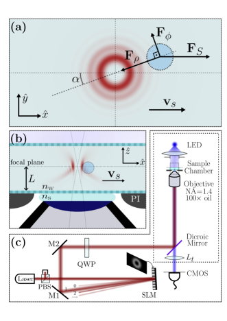
Figure 1: (a) A trapped particle is subject to a constant drag force $\mathbf{F}_{S}$ and finds a new off-axis equilibrium position rotated with respect to the direction of this force by an angle $\alpha$. $\mathbf{F}_{\rho}$ and $\mathbf{F}_{\phi}$ denote cylindrical optical force components, and $\mathbf{v}_{S}$ represents the fluid velocity. (b) Lateral view of the sample region showing the density plot (red) of the electric energy density for the nonparaxial focused beam. $L$ denotes the height of the paraxial focal plane with respect to the coverslip. PI represents the piezoelectric nano-positioning system used to move the microscope stage. (c) Schematic representation of the experimental setup: The laser beam propagates through a polarizing beam splitter (PBS) towards the spatial light modulator (SLM). The resulting first order of diffraction crosses a quarter-wave plate (QWP) before entering the microscope (dotted frame). The beam is then focused by an oil-immersion objective into the sample chamber.

II Experimental setup and procedure

Our method for radius measurements goes as follows. We apply a constant Stokes drag force $\mathbf{F}_{S}$ on a sphere trapped by optical tweezers with a given Laguerre-Gaussian mode LG${}_{p\ell},$ with radial order $p=0$ and topological charge $\ell,$ at the objective entrance port. The particle is displaced until it finds an off-axis equilibrium position rotated by an angle $\alpha$ with respect to the direction of the drag force, as depicted in Figs. 1(a) and (b). Then, we vary the topological charge, measuring rotation angles as a discrete function of $\ell$. Finally, we fit this data to the theoretical model presented in the next section, leaving the radius as a free parameter and, in some cases, also the astigmatism parameters and the paraxial focal height.

The experimental setup for the measurements of $\alpha$ is illustrated in Fig. 1(c). A $\rm TEM_{00}$ laser beam (IPG photonics, model YLR-5-1064LP) with vacuum wavelength $\lambda_{0}=1064\,\mathrm{nm}$ illuminates a spatial light modulator (SLM). This device enables the modulation of both the field’s amplitude and phase [22], which allows us to convert the incident beam into chosen $\text{LG}_{0\ell}$ modes with appropriate waist $w_{0}$ via a complex phase modulation. Notice that we choose a different beam waist for each mode so as to ensure an appropriate filling at the objective’s entrance. The criteria for choosing the waists and the method to measure them are described in Appendix A, while the waist values are given in Table 5. Before entering an inverted microscope, the beam is left-polarized by a quarter-wave plate. It is then focused by a $100\times$, oil-immersion objective with numerical aperture $\rm NA=1.4$ and back aperture radius $R_{\rm obj}=2.8\,\rm mm$ through the glass-water interface into an aqueous dispersion of polystyrene beads (Polysciences), where the optical trapping occurs (see Fig. 1(b)). This solution is illuminated by a 470 nm blue LED whose scattered light, after being collected by the objective, is recollimated by a tube lens ($L_{t}$) to form an image on a CMOS camera (Hamamatsu Orca-Flash 2.8 C11440-10C).

After trapping a microsphere with a focused Gaussian beam ($\ell=0$), we first lower the objective until the microsphere touches the bottom of the sample chamber. Then, we move up the objective by a height of $d=(2\pm 1)\,\upmu\mathrm{m}$ so as to define a new trapping position a few microns above the coverslip. To apply a constant drag force, we use a piezoelectric nano-positioning stage (Digital Piezo Controller E-710, Physik Instrumente) to move the microscope stage with the velocity ${\bf v}_{S}=\pm v_{S}\,\mathbf{\hat{x}},$ $v_{S}=20\,\upmu{\rm m/s},$ for 0.5 s, alternating between the positive and negative $x$ directions. At each cycle, the Stokes drag force displaces the particle from its on-axis equilibrium position. In a given run, the bead’s movement is recorded for 10 s. The center-of-mass position on the $xy$-plane at each frame is later determined by video analysis with Fiji [23], as depicted by way of example for the $x$ coordinate in the upper panel of Fig. 2.

The camera itself is rotated by an angle close to $45^{\circ}$ to ensure that the displacements along the $x$ and $y$ directions are roughly of the same magnitude. The central panel in Fig. 2 depicts all particle positions obtained from the measured $x$ coordinates shown in the upper panel as well as from the corresponding $y$ coordinates (not shown) for a typical run. All recorded positions are categorized into three separate clusters by means of a Scikit-learn routine [24] and marked as blue, green, and orange points in Fig. 2. In this way, the orange points that lie in between the two main clusters are identified and no longer considered for the analysis.

The marginal distributions for the $x$ and $y$ directions can be fairly described by Gaussian distributions so that we fit the two main clusters to two-dimensional Gaussians in order to determine the coordinates of the two equilibrium positions. We then obtain the angle depicted in Fig. 2 between the line connecting the two equilibrium positions and the $x$ direction. Its error is computed by propagating the error of the coordinates. Finally, to determine the rotation angle $\alpha$ depicted in Fig. 1(a), we subtract the camera offset angle, which is determined by recording the position of a fixed reference spot in the coverslip as the microscope stage is driven.

Apart from the rotation angle, we also extract the radial displacement $\rho_{\rm eq}$ of the sphere from the focal point. By assuming that the movement of the bead is symmetric, we can compute the displacement from the distance between the two equilibrium positions.

For each beam mode $\ell$ the measurement was repeated several times.

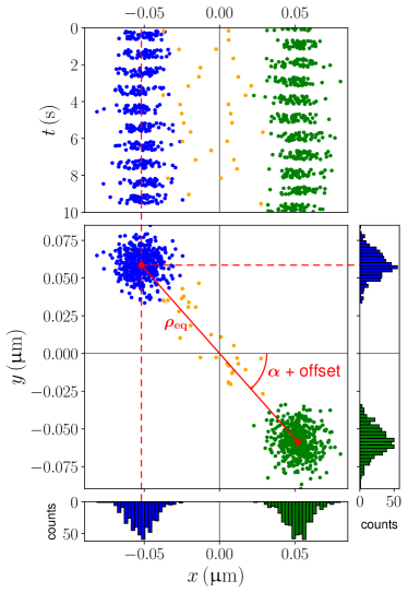
Figure 2: The $x$ and $y$ coordinates of the bead are measured over a time of $T=10\,\mathrm{s}$. The upper panel shows a typical distribution of the measured $x$ coordinates. Green and blue clusters correspond to opposite velocities of the microscope stage. The central panel shows the measured positions on the $xy$ plane. The histograms for the $x$ and $y$ coordinates are fitted by Gaussian functions in order to determine the equilibrium positions under the Stokes force (red points). The rotation angle $\alpha$ is then obtained from the slope of the red line connecting the two equilibrium positions.

III MDSA+ theory of the optical force by a focused vortex beam

The optical force acting on an illuminated particle is generally computed by integrating the time-averaged Maxwell stress tensor over a surface which encloses the particle. The stress tensor includes the incident and scattered field contributions. Within the Mie-Debye theory [25, 26], the former is described by a Debye-type nonparaxial model [20] for a tightly focused beam, while the latter follows from standard Mie scattering by a spherical particle. An extension to include the spherical aberration introduced by focusing through the glass-water planar interface led to the MDSA (Mie-Debye with spherical aberration) theory [27, 28]. In [29], the model was further extended (MDSA+ theory) to allow for the presence of any primary aberration on the paraxial Gaussian beam before focusing.

To mimic the experimental setup discussed in Sec. II, here we consider that the laser beam at the objective entrance port is a Laguerre-Gaussian mode LG${}_{0\ell}.$ Expressions for the aplanatic focusing of a Laguerre-Gaussian beam were developed in [30]. Building on these earlier results, we find the following angular spectrum decomposition for the electric field in the aqueous solution obtained from focusing a circularly polarized LG_0ℓ beam at the objective entrance port:

$$\mathbf{E}^{(\sigma)}_{\ell}(\mathbf{r}) =-\frac{ikfE_{0}e^{-ikf}}{2\pi}\left(\sqrt{2}\gamma\right)^{|\ell|}\int_{0}^{2\pi}d\varphi\,e^{i\ell\varphi}$$ (1)

$$\quad\times\int_{0}^{\theta_{m}}d\theta\,\sin\theta\sqrt{\cos\theta}\sin^{|\ell|}(\theta)e^{-\gamma^{2}\sin^{2}\theta}$$

$$\hskip 40.00006pt\times T(\theta)e^{i(\Psi_{\text{g-w}}+\Psi_{\text{ast}})}e^{i\mathbf{k}_{\text{w}}\cdot\mathbf{r}}\hat{\epsilon}_{\sigma}(\theta_{\text{w}},\varphi_{\text{w}})\,.$$

The spherical components $(k,\theta,\varphi)$ describe the wave vectors in the glass slide. The parameter $\gamma=f/w_{0}$ defines the ratio of the objective focal length $f$ and the beam waist $w_{0}$ at the objective entrance port. The polar angle $\theta_{\text{w}}$ in the host medium is defined through Snell’s law: $\sin\theta_{\text{w}}=\sin\theta/N_{\text{s}}$ where $N_{\text{s}}=n_{\text{w}}/n_{\text{s}}$ is the relative refractive index between the fluid and the glass slide. The integration is performed up to a maximum angle $\theta_{\text{m}}$ given by $\sin\theta_{\text{m}}=\text{min}\left(N_{\text{s}},\sin\theta_{0}\right)$ with $\sin\theta_{0}=\mathrm{NA}/n_{\text{w}}$, where NA denotes the numerical aperture of the objective. The wave vector $\mathbf{k}_{\text{w}}$ in the sample is characterized by its modulus $k_{\text{w}}=N_{\text{s}}k$ and the spherical angles $(\theta_{\text{w}},\varphi_{\text{w}})$ where $\varphi_{\text{w}}=\varphi$. The unit vector $\hat{\epsilon}_{\sigma}(\theta_{\text{w}},\varphi_{\text{w}})=e^{i\sigma\varphi_{\text{w}}}(\hat{\theta}_{\text{w}}+i\sigma\hat{\varphi}_{\text{w}})/\sqrt{2}$ accounts for a right- ($\sigma=-1$) or left-handed ($\sigma=1$) circularly polarized Fourier component along the propagation direction $(\theta_{\text{w}},\varphi_{\text{w}}).$ It is obtained by rotating the unit vector $(\hat{x}+i\sigma\hat{y})/\sqrt{2}$ at the entrance of the objective by the Euler angles $(\varphi_{\text{w}},\theta_{\text{w}},-\varphi_{\text{w}}).$

The astigmatism (ast) introduced by the optical elements of the experimental setup is accounted for by the Zernike phase [31, 32]

$$\Psi_{\text{ast}}=2\pi A_{\text{ast}}\left(\frac{\sin\theta}{\sin\theta_{0}}\right)^{2}\cos\left[2(\varphi-\phi_{\text{ast}})\right]$$ (2)

given in terms of the amplitude $A_{\text{ast}}$ and of the angle $\phi_{\text{ast}}$ defining the astigmatism axis and thus breaking rotational symmetry.

We also take into account the spherical aberration introduced by refraction at the interface between the coverslip and the aqueous suspension. Neglecting the dependence of the Fresnel refraction coefficients on the polarization, the transmission amplitude is [27]

$$T(\theta)=\frac{2\cos\theta}{\cos\theta+N_{\text{s}}\cos\theta_{\text{w}}}$$ (3)

whereas the spherical aberration phase reads [33]

$$\Psi_{\text{g-w}}=kL\left(N_{\text{s}}\cos\theta_{\text{w}}-\frac{\cos\theta}{N_{\text{s}}}\right)$$ (4)

where $L$ is the distance between the glass-water (g-w) interface and the paraxial focus as illustrated in Fig. 1(b).

The incident field (1) is inserted into the Maxwell stress tensor together with the scattered field, which is obtained by solving the scattering problem using Mie theory for spherical particles combined with the appropriate Wigner rotation matrix elements. The integration over the stress tensor can be worked out analytically. Explicit expressions for the cylindrical force components ($F_{\rho},F_{\phi},F_{z}$) as functions of the position of the sphere center $\mathbf{R}(\rho,\phi,z)$ with respect to the focus can be found in Appendix B.

IV Results and discussion

IV.1 Numerical analysis

The sphere radius $R$ as well as the parameters for the optical aberrations can be obtained by fitting the experimental data with the rotation angles obtained from the MDSA+ theory. Two optical aberrations are considered in our model. The first one is the spherical aberration produced at the glass-water interface, which is characterized by the phase (4) proportional to the distance $L$ of the paraxial focus from the coverslip. The second is astigmatism, defined by (2) in terms of the amplitude $A_{\text{ast}}$ and the angle of the principal meridian $\phi_{\text{ast}}$. The distance $L$ can, in principle, be determined by emulating the experimental procedure described in Sec. II [27]. Considering a Gaussian mode at the entrance of the objective, we first compute the initial focal height $L_{0}$ for which the on-axis equilibrium position is such that the sphere is touching the coverslip. The equilibrium position is obtained from the requirement of a vanishing axial force component

$$F_{z}^{(\ell=0)}\left(\rho=0,\phi=0,z=R-L_{0},L=L_{0}\right)=0\,.$$ (5)

Afterwards, the focal plane is displaced upwards by $d$ leading to the final height $L=L_{0}+N_{s}d$. The rotation angle for each mode $\ell$ can then be found by solving the following system of equations for the equilibrium position $\mathbf{R}_{\text{eq}}=\mathbf{R}_{\text{eq}}(\rho_{\text{eq}},\alpha,z_{\text{eq}})$ under the applied Stokes drag force:

$$F_{z}^{(\ell)}(\mathbf{R}_{\text{eq}}) =0$$ (6)

$$\arctan\left(\frac{F_{\phi}^{(\ell)}(\mathbf{R}_{\text{eq}})}{F_{\rho}^{(\ell)}(\mathbf{R}_{\text{eq}})}\right) =\alpha$$

with the force expressions given in Appendix B. The rotation angle $\alpha$ corresponds to the azimuth angle $\phi$ of the bead at its equilibrium position. The radial component $\rho_{\text{eq}}$ is extracted from the experimental data as described in the previous section. We found that the rotation angle only weakly depends on $\rho_{\text{eq}}$, meaning that the changes in the rotation angle with the radial distance are negligible. For each $\text{LG}_{0\ell}$ mode, we thus average $\rho_{\text{eq}}$ over all measurement runs for a given bead and use the resulting average value as input for the radial equilibrium coordinate.

Note that without astigmatism ($A_{\text{ast}}=0$) the force components do not explicitly depend on the azimuthal angle $\phi$. Hence, the set of equations (6) no longer needs to be solved simultaneously. Instead, after determining the axial equilibrium position, we can directly calculate the rotation angle. The computation time using only the MDSA theory is thus significantly reduced compared to the full calculation within the MDSA+ theory.

The fitting is done by minimizing a weighted sum of squared errors between the theoretical and experimental results for the rotation angle

$$\chi^{2}=\frac{1}{N}\sum_{\ell}\frac{1}{M_{\ell}}\sum_{r}\left(\frac{\alpha(\ell)-\alpha_{\text{exp}}(\ell,r)}{\Delta\alpha_{\text{exp}}(\ell,r)}\right)^{2}$$ (7)

where $\alpha_{\text{exp}}(\ell,r)\pm\Delta\alpha_{\text{exp}}(\ell,r)$ is the experimentally obtained rotation angle and its error for the beam mode $\ell$ and run $r$, $N$ is the number of modes used for fitting and $M_{\ell}$ is the number of measurement rounds performed for each beam mode. The maximum number of runs $M_{\ell}$ was ten, while in a few cases, due to experimental reasons, only data from one run could be used.

The force calculation was implemented in Python using the scientific libraries NumPy [34] and SciPy [35]. For the minimization of $\chi^{2}$ we used the iminuit package [36].

Relevant parameters for the simulations not yet mentioned include the refractive index of the immersion oil $n_{\text{s}}=1.518$ and the refractive index of the polystyrene beads $n=1.5694$, which we obtained by linearly interpolating the data given in [37] to our wavelength of $\lambda_{0}=1064\,$nm. The laser power, below $120\,{\rm mW}$ at the objective entrance port, is too low to heat the sample. Therefore, we assume it to be in thermal equilibrium with its environment and use the refractive index for water $n_{\text{w}}=1.3246$ at $T=19\,^{\circ}$C in our calculations. For comparison, we also performed the calculation for $T=24\,^{\circ}$C with $n_{\text{w}}=1.3242$ and found no significant change in the fitted parameters. These refractive indices for $\lambda_{0}$ were obtained from a linear interpolation of the data given in [38].

IV.2 Beads of nominal radius 1.5 microns

We begin by discussing the results for two beads whose nominal radius is $(1.50\pm 0.04)\,\upmu\mathrm{m}$. In the following, we refer to them as beads A and B. Fig. 3 shows the experimental results for the rotation angles of each bead for beam modes ranging from $\ell=-4$ to $\ell=4$. The error bars are the standard deviations of $\alpha$ computed from the multiple rounds of measurement.

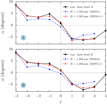
Figure 3: Microsphere rotation angle $\alpha$ versus beam mode $\ell$ for beads A and B. The circles depict the experimental results and the squares and triangles are the result of fitting with MDSA and MDSA+ theories, respectively, with the latter including the effect of astigmatism. In all plots, we have added lines connecting the data points as a guide to the eye.

For each sphere, we performed a fit, where we excluded the $\ell=4$ case for which we found no reasonable value for $\alpha$. We believe that the reason for this is that $\ell=4$ is close to the bistable trapping regime demonstrated in Ref. [11]. Although the bead does have stability around the axis, it also probes a region of positive torque near the annular focal spot, due to its thermal fluctuations. This causes the experimental value of $\alpha$ to be much less negative than the value of about $-15.7^{\circ}$ predicted by theory.

First, we fitted the experimental curve by just using the MDSA theory with $L$ determined as described above. The fitted radii can be found in Tab. 1 and $\alpha$ as a function of $\ell$ is depicted in Fig. 3. Overall, the fitted data points show good qualitative agreement with the experimental result, except for $\ell=0$. In this case, theory predicts a negative rotation angle, while the experimentally observed one is positive. We will discuss the reason for this discrepancy below.

Table 1: Optimal radii for beads of nominal radius $(1.50\pm 0.04)\,\upmu\mathrm{m}$ from a fit within the MDSA theory (zero astigmatism).

bead	$R(\upmu\mathrm{m})$	$\chi^{2}$
A	1.500 $\pm$ 0.004	21.7
B	1.494 $\pm$ 0.003	26.4

Next, we used the MDSA+ theory for fitting with $A_{\text{ast}}$, $\phi_{\text{ast}}$ and $L$ as additional parameters. The parameters obtained from the fit can be found in Tab. 2. The fitted data points depicted in Fig. 3 show almost perfect agreement with the experimental results. Notice that the $\chi^{2}$ value does not indicate overfitting. In addition, in spite of the large number of parameters, the two independent fits for beads A and B found astigmatism parameters $A_{\text{ast}}$ and $\phi_{\text{ast}}$ that agree within error bars. This is to be expected since the astigmatism is a characteristic of the experimental setup, thus remaining the same for measurements with both beads. On the other hand, the difference of about 1 $\upmu\mathrm{m}$ between the values of $L$ for the two beads is still consistent with the large error of adjusting the height of the objective as mentioned in Sec. II. Following this reasoning, we also performed a joint fit for beads A and B with shared parameters for the astigmatism. The results can be found in Tab. 3.

As for the fitted radii, notice that they are close to the ones found by fitting the data to the MDSA theory. This shows that if one wishes solely to characterize a bead’s radius, the method can be performed with this simpler version of the theory, drastically reducing the necessary computation time. Furthermore, we have performed the MDSA-fit with each individual round and found values for the radius compatible with the ones in Tab. 1, suggesting that the method could be greatly simplified.

Table 2: Fit parameters for beads of nominal radius $(1.50\pm 0.04)\,\upmu\mathrm{m}$.

bead	$R(\upmu\mathrm{m})$	$L(\upmu\mathrm{m})$	$A_{\text{ast}}$	$\phi_{\text{ast}}\text{(rad)}$	$\chi^{2}$
A	1.503 $\pm$ 0.007	5.8 $\pm$ 0.6	0.245 $\pm$ 0.026	0.37 $\pm$ 0.14	2.2
B	1.492 $\pm$ 0.005	4.7 $\pm$ 0.6	0.262 $\pm$ 0.024	0.44 $\pm$ 0.12	2.3

It should be noted that only the presence of higher-order modes allows the distinction between spheres A and B. The measured rotation angles for a Gaussian mode are $\alpha_{\mathrm{A}}(\ell=0)=(0.7\pm 0.2)^{\circ}$ and $\alpha_{\mathrm{B}}(\ell=0)=(1.1\pm 0.4)^{\circ}$ respectively for beads A and B. They are practically indistinguishable within error bars. However, if we now look at the case $\ell=2$, the corresponding results are $\alpha_{\mathrm{A}}(\ell=2)=(-6.3\pm 0.1)^{\circ}$ and $\alpha_{\mathrm{B}}(\ell=2)=(-7.3\pm 0.1)^{\circ}$. Note that in that case not only are the values further apart, but they are distinguishable beyond error bars.

Finally, we emphasize that for all modes except $\ell=0$ the angular momentum gained by the particle is opposite to that carried by the paraxial beam. This exception happens because for this mode the total angular momentum per photon is relatively small, and the symmetry-breaking effect of astigmatism dominates over the angular momentum exchange. This is corroborated by $\ell=-1$, where the total angular momentum per photon is zero, and the torque, caused exclusively by the spot-asymmetry, is positive. Therefore, the negative optical torque reported in [6] extends to $\rm LG_{0\ell}$ modes and seems to be a characteristic of near-focus interactions, rather than a particularity of that setup.

Table 3: Parameters from the joint fit for two beads with nominal radius $(1.50\pm 0.04)\,\upmu\mathrm{m}$ using shared values for the astigmatism.

$R_{A}(\upmu\mathrm{m})$	$R_{B}(\upmu\mathrm{m})$	$L_{A}(\upmu\mathrm{m})$	$L_{B}(\upmu\mathrm{m})$	$A_{\text{ast}}$	$\phi_{\text{ast}}\text{(rad)}$	$\chi^{2}_{A,B}$
1.502 $\pm$ 0.010	1.492 $\pm$ 0.007	5.56 $\pm$ 0.83	4.85 $\pm$ 0.78	0.254 $\pm$ 0.026	0.41 $\pm$ 0.14	2.4, 2.4

IV.3 Beads of nominal radius 2.260 microns

We now discuss the results for two beads whose radii have a nominal value of $R_{\mathrm{N}}=(2.260\pm 0.075)\,\upmu\mathrm{m}$ and are referred to as beads C and D in the following. Due to their larger size, these beads were stably trapped on the optical axis for a broader range of topological charges [11] when compared to the smaller beads discussed above. The experiments were performed with $\ell$ ranging from $-7$ to $7$ yielding the data shown in Fig. 4. Beads in the geometrical optics regime $R\gg\lambda$ are less sensitive to optical aberrations because the asymmetries in the field distribution are averaged out over the sphere. We thus neglect the astigmatism and use fixed values for the distance $L$ as determined from the known displacement $d$ of the objective when fitting the experimental data.

The experimental data for $\ell$ ranging from $-6$ to $6$ were fitted. In the cases $\ell=\pm 7$, we could not find equilibrium positions for all radii in the fitting interval ranging from 2.11 to 2.41 $\upmu$m. We believe that the explanation lies again in the size of the annular focal spot, which is too large to allow for stable trapping on the beam axis for the highest values of $|\ell|$. The radii obtained from the fit are given in Tab. 4 and the fitted data for $\alpha$ are depicted in Fig. 4. For comparison, we also performed the fit using the MDSA+ theory with the astigmatism parameters obtained from the joint fit of beads A and B. The resulting radii lay within the error bars of the radii obtained within the MDSA theory and the quality of the fit shows no significant improvement. Due to the high relative error of measuring the displacement $d$, we also performed the fit with $d=3\,\mu\mathrm{m}$ which again leads to the same optimal radii. Our findings thus confirm that both astigmatism and spherical aberration are less critical for larger spheres, which implies that here the fitting process is even more robust than for smaller spheres.

The sensitivity of our method with respect to changes in the radii can be inferred from Fig. 4, where the rotation angles are also depicted for the nominal radius $R_{\mathrm{N}}$. The agreement with the experimental data becomes much worse in this case and the qualitative aspects of the curve change, with even an opposite sign for the rotation angles for modes with topological charges in the range $-3\leq\ell\leq 2$.

Table 4: Optimal radii for beads of nominal radius $(2.260\pm 0.075)\,\upmu\mathrm{m}$.

bead	$R(\upmu\mathrm{m})$	$\chi^{2}$
C	2.339 $\pm$ 0.003	40.1
D	2.331 $\pm$ 0.003	67.7

Fig. 5 displays $\chi^{2}$ as a function of the sphere radius for bead A (upper panel) and beads C and D (lower panel). Notice that the curves for beads C and D do not only exhibit a minimum at the optimal fit but also possess local minima at other values of the radius. The height of the dashed and dotted line serves as a reference for comparison with $\chi^{2}$ for the optimal fit. The grey area indicates the error interval around the nominal radius. The observed pseudo-oscillations originate in the semi-classical scattering limit from the interference between direct reflection and radial round-trip propagation inside the sphere over a distance $4R$ [25], and their period is given by $\lambda_{0}/4n\approx 0.169\,\upmu\mathrm{m}$. The distance between the first two and the last two minima is found for bead C as $0.170\,\upmu\mathrm{m}$ and $0.171\,\upmu\mathrm{m}$, respectively, and for bead D as $0.164\,\upmu\mathrm{m}$ and $0.172\,\upmu\mathrm{m}$, respectively. These values are close to the theoretically expected period considering the error bars of the fitted radii.

The ambiguity arising from multiple minima does not have an impact on the results for bead A, as indicated in the upper panel of Fig. 5. Since its radius is closer to the wavelength of the trapping light, the interference effect described above is not as pronounced as in the case of the larger spheres C and D. Consequently, their fitted radii values correspond to more clearly defined global minima.

As for beads C and D, the radii given in Table 4 correspond to the global minima of $\chi^{2}$ and they lie closer to the nominal value than radii associated with additional local minima of $\chi^{2}$. The minima displayed in the lower panel of Fig. 5 at radii beyond $2.5\,\upmu\mathrm{m}$ have values of $\chi^{2}$ comparable to the global minima as can be seen by means of the horizontal lines. However, these radii differ from the nominal value by more than $3\sigma$ and therefore should be excluded. Even though the local minima of $\chi^{2}$ at a radius around $2.17\,\upmu\mathrm{m}$ clearly lie above the respective global minimum, we need to assess whether the difference between the two values of $\chi^{2}$ is significant. To this end, we consider the maximum of $\chi^{2}$ within the error interval of the fitted radii according to Table 4. For bead C, we find a maximal value of $41.2$ as compared to the value of $48.1$ at a radius of $2.169\,\upmu\mathrm{m}$. Therefore, the global minimum is significantly better than the local minimum. A similar analysis can be carried out for bead D confirming that also in this case the global minimum is indeed significantly better.

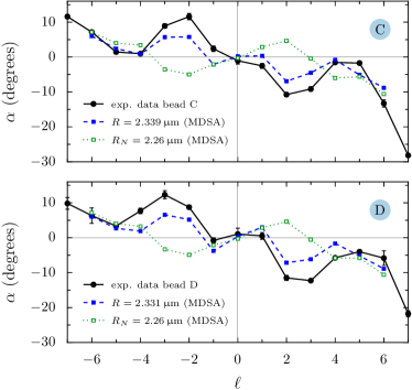
Figure 4: Rotation angles for beads C and D as functions of the beam mode $\ell$. The circles depict the experimental results. The fitted data from the MDSA theory is shown in blue. The values at $\ell=\pm 7$ were excluded from the fit. As in Fig. 3, the lines connecting the data points serve as a visual aid.

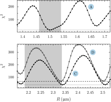
Figure 5: In the bottom panel, $\chi^{2}$ as a function of the radius $R$ for beads C (circles) and D (squares) is shown within the MDSA theory. The grey area depicts the error interval for the nominal radius $(2.260\pm 0.075)\,\upmu\mathrm{m}$ provided by the bead manufacturer. The dotted (dashed) line shows the value of $\chi^{2}$ for bead C (D) found from the fit and given in Tab. 4. The top panel shows, for comparison, $\chi^{2}$ for bead A. The grey area represents the error interval $(1.50\pm 0.04)\,\upmu\mathrm{m}$.

V Conclusions

In conclusion, we have presented a method for determining the radii of optically trapped microspheres with errors on the order of a nanometer, well below the usual manufacturer’s standard error. One of its main advantages is that it allows to measure a specific spherical particle in situ during trapping experiments.

Furthermore, we showed that micro-sized particles with $R\approx\lambda$ can be used to probe the optical aberrations of the experimental setup as well as to get an estimate for the height of the sphere above the coverslip, which is an experimental parameter hard to determine with precision.

Appendix A Waist and Objective Filling

To ensure good trapping conditions in optical tweezers, one must guarantee that the waist of the paraxial beam is such that it illuminates the objective entrance with a significant fraction of its power distributed near the border of the lenses. In this way the marginal rays are strongly deflected, optimizing the focused beam’s intensity gradient. For a Gaussian beam, this means simply overfilling the entrance. However, Laguerre-Gaussian beams require a more careful choice of waist, since most of its power is localized far from the optical axis and may leak outside the objective if the beam waist is too large. In the experiments presented here, we have used two criteria for the choice of each mode’s waist. One is the theoretical criterion presented in [11] to control the objective filling by the ratio $r_{\ell}/R_{\rm obj}$, where $r_{\ell}$ is the radius of maximum intensity of the paraxial $\rm LG_{0\ell}$ beam. The second criterion was empirical, based on the limitations of the SLM. As the topological charge increases, the modulation masks necessary to reduce the beam’s waist become larger, to the point that they can no longer fit inside the SLM’s display. Hence, one must choose waist values that sufficiently optimize the optical tweezers’ intensity gradient and, at the same time, are produced by masks that fit inside the SLM’s display.

To experimentally measure the waist values of each Laguerre-Gaussian mode, we have employed a variation of the method described in [27]. It consists of measuring the power through a diaphragm of radius $a$ centered at the beam’s axis as a function of this aperture, and then fitting the power to the integrated intensity in the diaphragm’s area. In the case of a Laguerre-Gaussian mode, we have:

$$P_{\ell}(R)=P_{t}\left[\Gamma(|\ell|+1)-\Gamma\left(|\ell|+1,\frac{2a^{2}}{w_{0}^{2}}\right)\right]$$ (8)

where $P_{t}=(\pi/2)w_{0}^{2}I_{0}$ is the total beam power in the $\ell=0$ (Gaussian) case. Instead of an actual diaphragm, we have simulated its effect by using the spatial light modulator to divert all light outside a circle with controllable radius $R$ centered at the beam axis. The measured waist values and the ratio $r_{\ell}/R_{\text{obj}}$ for each mode are presented in Table  5.

Table 5: Measured waist for each $\text{LG}_{0\ell}$ mode

$\ell$	$w_{0}\,(\mathrm{mm})$	$r_{\ell}/R_{\rm obj}$
0	$2.150\pm 0.004$	-
$\pm 1$	$1.732\pm 0.008$	$0.44$
$\pm 2$	$1.204\pm 0.004$	$0.43$
$\pm 3$	$1.171\pm 0.005$	$0.51$
$\pm 4$	$1.039\pm 0.007$	$0.52$
$\pm 5$	$0.948\pm 0.003$	$0.54$
$\pm 6$	$0.867\pm 0.002$	$0.54$
$\pm 7$	$0.806\pm 0.002$	$0.54$

Appendix B Multipole expansion of the optical force

Here, we present the series expansion of the optical force components for a Laguerre-Gaussian beam within the MDSA+ theory [29].

We use a dimensionless force $\mathbf{Q}=\mathbf{F}/(n_{\text{w}}P/c)$, with the laser beam power $P$, the speed of light $c$ and the refractive index in the sample region $n_{\text{w}}$. The force is given by subtracting the loss at the sphere (-$\mathbf{Q}_{s}$) from the total extinction ($\mathbf{Q}_{e}$)

$$\mathbf{Q}(\mathbf{R})=\mathbf{Q}_{s}+\mathbf{Q}_{e}$$ (9)

and it is calculated at the position $\mathbf{R}=\mathbf{R}(\rho,\phi,z)$ of the spherical particle with respect to the focal spot.

First, we present the components of the scattering force. The axial part of the scattering force is given by

$$Q_{sz}^{(\sigma,\ell)}=-\frac{8\gamma^{2}}{A_{\ell}N_{s}}\mathrm{Re}\sum\limits_{j=1}^{\infty}\sum_{m=-j}^{j} \left[\frac{\sqrt{j(j+2)(j-m+1)(j+m+1)}}{j+1}(a_{j}a_{j+1}^{*}+b_{j}b_{j+1}^{*})G_{j,m}^{(\sigma,\ell)}G_{j+1,m}^{(\sigma,\ell)*}\right.$$ (10)

$$\quad\left.+\sigma m\frac{2j+1}{j(j+1)}a_{j}b_{j}^{*}\left|G_{j,m}^{(\sigma,\ell)}\right|^{2}\right]$$

where $a_{j}$ and $b_{j}$ are the Mie coefficients and $A_{\ell}$ defines the so-called filling factor given by

$$A_{\ell}=8(2\gamma^{2})^{|\ell|+1}\int_{0}^{\sin\theta_{\text{m}}}t^{2|\ell|+1}e^{-2\gamma^{2}t^{2}}\frac{\sqrt{(1-t^{2})(N_{\text{s}}^{2}-t^{2})}}{\left(\sqrt{1-t^{2}}+\sqrt{N_{\text{s}}^{2}-t^{2}}\right)^{2}}\,\mathrm{d}t\,.$$ (11)

The transverse components of the scattering force are given by

$$\left\{\begin{array}[]{c}Q_{s\rho}^{(\sigma,\ell)}\\ Q_{s\phi}^{(\sigma,\ell)}\end{array}\right\}=\frac{4\gamma^{2}}{A_{\ell}N_{s}}\left\{\begin{array}[]{c}\mathrm{Im}\\ -\mathrm{Re}\end{array}\right\}\sum\limits_{j=1}^{\infty}\sum_{m=-j}^{j} \left[\frac{\sqrt{j(j+2)(j+m+1)(j+m+2)}}{j+1}(a_{j}a_{j+1}^{*}+b_{j}b_{j+1}^{*})\right.$$ (12)

$$\hskip 50.00008pt\times\left(G_{j,m}^{(\sigma,\ell)}G_{j+1,m+1}^{(\sigma,\ell)*}\pm G_{j,-m}^{(\sigma,\ell)}G_{j+1,-m-1}^{(\sigma,\ell)*}\right)$$

$$\quad-\left.2\sigma\frac{2j+1}{j(j+1)}\sqrt{(j-m)(j+m+1)}\mathrm{Re}(a_{j}b_{j}^{*})G_{j,m}^{(\sigma,\ell)}G_{j,m+1}^{(\sigma,\ell)*}\right]$$

where the upper sign corresponds to the radial force component, while the lower sign is for the azimuthal part. The multipole coefficients of the circularly polarized Laguerre-Gaussian beam, including optical aberrations, are given by

$$G_{j,m}^{(\sigma,\ell)}(\mathbf{R})=(\sqrt{2}\gamma)^{|\ell|}\int_{0}^{\theta_{m}}\mathrm{d}\theta\sqrt{\cos(\theta)}\sin^{|\ell|+1}(\theta)e^{-\gamma^{2}\sin^{2}(\theta)}d_{m,\sigma}^{j}(\theta_{w})f^{(\sigma,\ell)}_{m}(\mathbf{R})e^{ik_{w}\cos(\theta)z+i\Psi_{\text{g-w}}}\,.$$ (13)

The coefficient $f_{m}^{(\sigma,\ell)}$ accounts for the astigmatism. The explicit expression for a Gaussian beam can be found in Eq. (8) of [29] and for a Laguerre-Gaussian beam we obtained

$$f^{(\sigma,\ell)}_{m}(\mathbf{R})= \sum_{s=-\infty}^{\infty}(-i)^{s}J_{s}\left(2\pi A_{\text{ast}}\frac{\sin^{2}\theta}{\sin^{2}\theta_{0}}\right)$$ (14)

$$\times J_{2s+m-\sigma-\ell}(k\rho\sin\theta)e^{2is(\phi_{\text{ast}}-\phi)}\,.$$

In the absence of astigmatism $A_{\text{ast}}=0$, only the $s=0$ term contributes to the sum and the coefficient reduces to

$$f^{(\sigma,\ell)}_{m}(\mathbf{R})=J_{m-\sigma-\ell}(k\rho\sin\theta)\,.$$ (15)

Next, we present the expressions for the extinction force. The axial part is given by

$$Q_{ez}^{(\sigma,\ell)}=\frac{4\gamma^{2}}{A_{\ell}N_{s}}\mathrm{Re}\sum\limits_{j,m}(2j+1)(a_{j}+b_{j})G_{j,m}^{(\sigma,\ell)}\left(G^{(\sigma,\ell)^{\prime}}_{j,m}\right)^{*}.$$ (16)

The coefficient $G^{(\sigma,\ell)^{\prime}}_{j,m}$ can be expressed in terms of the multipole coefficients (13) by applying the recursion relation for Wigner-$d$ matrix elements [39, p. 90]

$$G^{(\sigma,\ell)^{\prime}}_{j,m}=\frac{\sqrt{j(j+2)\left[(j+1)^{2}-m^{2}\right]}}{(2j+1)(j+1)}G_{j+1,m}^{(\sigma,\ell)}+\frac{\sqrt{(j^{2}-m^{2})(j^{2}-1)}}{j(2j+1)}G_{j-1,m}^{(\sigma,\ell)}+\sigma\frac{m}{j(j+1)}G_{l,m}^{(\sigma,\ell)}\,.$$ (17)

The transverse components of $\mathbf{Q}_{\mathrm{e}}$ are given by

$$\left\{\begin{array}[]{c}Q_{e\rho}^{(\sigma,\ell)}\\ Q_{e\phi}^{(\sigma,\ell)}\end{array}\right\}=\frac{2\gamma^{2}}{A_{\ell}N_{s}}\left\{\begin{array}[]{c}\mathrm{Im}\\ -\mathrm{Re}\end{array}\right\}\sum\limits_{j,m}(2j+1)(a_{j}+b_{j})G_{j,m}^{(\sigma,\ell)}\left(G^{-,(\sigma,\ell)}_{j,m+1}\mp G^{+,(\sigma,\ell)}_{j,m-1}\right)^{*}\,.$$ (18)

The negative (positive) sign corresponds to the radial (azimuthal) component. The multipole coefficients $G^{\pm,(\sigma,\ell)}_{j,m-1}$ can also be expressed in terms of the coefficients $G^{(\sigma,\ell)}_{j,m-1}$ by again applying recursion relations

$$G^{\pm,(\sigma,\ell)}_{j,m} =\mp\frac{\sqrt{(j\pm m)(j\pm m+1)(j^{2}-1)}}{j(2j+1)}G_{j-1,m}^{(\sigma,\ell)}+\sigma\frac{\sqrt{(j\mp m)(j\pm m+1)}}{j(j+1)}G_{j,m}^{(\sigma,\ell)}$$ (19)

$$\qquad\pm\frac{\sqrt{(j\mp m)(j\mp m+1)((j+1)^{2}-1)}}{(j+1)(2j+1)}G_{j+1,m}^{(\sigma,\ell)}\,.$$

Making use of the recursion relations (17) and (19) reduces drastically the need to explicitly evaluate integrals of the form (13) and thus significantly improves the runtime of the numerical calculations.

References

- Chen et al. [2014] J. Chen, J. Ng, K. Ding, K. H. Fung, Z. Lin, and C. T. Chan, Negative optical torque, Sci. Rep. 4, 6386 (2014).
- Canaguier-Durand and Genet [2015] A. Canaguier-Durand and C. Genet, Chiral route to pulling optical forces and left-handed optical torques, Phys. Rev. A 92, 043823 (2015).
- Hakobyan and Brasselet [2014] D. Hakobyan and E. Brasselet, Left-handed optical radiation torque, Nat. Photon. 8, 610 (2014).
- Magallanes and Brasselet [2018] H. Magallanes and E. Brasselet, Macroscopic direct observation of optical spin-dependent lateral forces and left-handed torques, Nat. Photon. 12, 461 (2018).
- Han et al. [2018] F. Han, J. A. Parker, Y. Yifat, C. Peterson, S. K. Gray, N. F. Scherer, and Z. Yan, Crossover from positive to negative optical torque in mesoscale optical matter, Nat. Commun. 9, 4897 (2018).
- Diniz et al. [2019] K. Diniz, R. S. Dutra, L. B. Pires, N. B. Viana, H. M. Nussenzveig, and P. A. Maia Neto, Negative optical torque on a microsphere in optical tweezers, Opt. Express 27, 5905 (2019).
- Parker et al. [2020] J. Parker, C. W. Peterson, Y. Yifat, S. A. Rice, Z. Yan, S. K. Gray, and N. F. Scherer, Optical matter machines: angular momentum conversion by collective modes in optically bound nanoparticle arrays, Optica 7, 1341 (2020).
- Qi et al. [2022] T. Qi, F. Han, W. Liu, and Z. Yan, Stable negative optical torque in optically bound nanoparticle dimers, Nano Lett. 22, 8482 (2022).
- Nan et al. [2022] F. Nan, X. Li, S. Zhang, J. Ng, and Z. Yan, Creating stable trapping force and switchable optical torque with tunable phase of light, Sci. Adv. 8, eadd6664 (2022).
- Curtis and Grier [2003] J. E. Curtis and D. G. Grier, Structure of optical vortices, Phys. Rev. Lett. 90, 133901 (2003).
- Fonseca et al. [2023] A. L. Fonseca, K. Diniz, P. B. Monteiro, L. B. Pires, G. T. Moura, M. Borges, R. S. Dutra, D. S. Ether Jr, N. B. Viana, and P. A. Maia Neto, Tailoring bistability in optical tweezers with vortex beams and spherical aberration, arXiv:2311.04737 (2023).
- Ali et al. [2020a] R. Ali, F. A. Pinheiro, R. S. Dutra, F. S. S. Rosa, and P. A. Maia Neto, Probing the optical chiral response of single nanoparticles with optical tweezers, J. Opt. Soc. Am. B 37, 2796 (2020a).
- Ali et al. [2020b] R. Ali, F. A. Pinheiro, R. S. Dutra, F. S. S. Rosa, and P. A. Maia Neto, Enantioselective manipulation of single chiral nanoparticles using optical tweezers, Nanoscale 12, 5031 (2020b).
- Allen et al. [1992] L. Allen, M. W. Beijersbergen, R. J. C. Spreeuw, and J. P. Woerdman, Orbital angular momentum of light and the transformation of Laguerre-Gaussian laser modes, Phys. Rev. A 45, 8185 (1992).
- Burnham and McGloin [2009] D. R. Burnham and D. McGloin, Radius measurements of optically trapped aerosols through Brownian motion, New J. Phys. 11, 063022 (2009).
- Preston and Reid [2015] T. C. Preston and J. P. Reid, Determining the size and refractive index of microspheres using the mode assignments from Mie resonances, J. Opt. Soc. Am. A 32, 2210 (2015).
- McGrory et al. [2020] M. R. McGrory, M. D. King, and A. D. Ward, Using Mie scattering to determine the wavelength-dependent refractive index of polystyrene beads with changing temperature, J. Phys. Chem. A 124, 9617 (2020).
- Pecora [2000] R. Pecora, Dynamic light scattering measurement of nanometer particles in liquids, J. Nanopart. Res. 2, 123 (2000).
- Gómez et al. [2021] F. Gómez, R. S. Dutra, L. B. Pires, G. R. de S. Araújo, B. Pontes, P. A. Maia Neto, H. M. Nussenzveig, and N. Viana, Nonparaxial Mie theory of image formation in optical microscopes and characterization of colloidal particles, Phys. Rev. Appl. 15, 064012 (2021).
- Richards and Wolf [1959] B. Richards and E. Wolf, Electromagnetic diffraction in optical systems. II. Structure of the image field in an aplanatic system, Proc. R. Soc. Lond. A 253, 358 (1959).
- Dutra et al. [2012] R. S. Dutra, N. B. Viana, P. A. Maia Neto, and H. M. Nussenzveig, Absolute calibration of optical tweezers including aberrations, Appl. Phys. Lett. 100, 131115 (2012).
- Rosales-Guzmán and Forbes [2017] C. Rosales-Guzmán and A. Forbes, How to shape light with spatial light modulators (SPIE Press, 2017).
- Schindelin et al. [2012] J. Schindelin, I. Arganda‐Carreras, E. Frise, V. Kaynig, M. Longair, T. Pietzsch, S. Preibisch, C. T. Rueden, S. Saalfeld, S. Saalfeld, B. Schmid, J. Tinevez, D. J. White, V. Hartenstein, K. W. Eliceiri, P. Tomancak, and A. Cardona, Fiji: an open-source platform for biological-image analysis, Nat. Methods 9, 676 (2012).
- Pedregosa et al. [2011] F. Pedregosa, G. Varoquaux, A. Gramfort, V. Michel, B. Thirion, O. Grisel, M. Blondel, P. Prettenhofer, R. Weiss, V. Dubourg, J. Vanderplas, A. Passos, D. Cournapeau, M. Brucher, M. Perrot, and E. Duchesnay, Scikit-learn: Machine learning in Python, J. Mach. Learn. Res. 12, 2825 (2011).
- Maia Neto and Nussenzveig [2000] P. A. Maia Neto and H. M. Nussenzveig, Theory of optical tweezers, EPL 50, 702 (2000).
- Mazolli et al. [2003] A. Mazolli, P. A. Maia Neto, and H. M. Nussenzveig, Theory of trapping forces in optical tweezers, Proc. R. Soc. Lond. A 459, 3021 (2003).
- Viana et al. [2007] N. B. Viana, M. S. Rocha, O. N. Mesquita, A. Mazolli, P. A. Maia Neto, and H. M. Nussenzveig, Towards absolute calibration of optical tweezers, Phys. Rev. E 75, 021914 (2007).
- Dutra et al. [2007] R. S. Dutra, N. B. Viana, P. A. Maia Neto, and H. M. Nussenzveig, Polarization effects in optical tweezers, J. Opt. A 9, S221 (2007).
- Dutra et al. [2014] R. S. Dutra, N. B. Viana, P. A. Maia Neto, and H. M. Nussenzveig, Absolute calibration of forces in optical tweezers, Phys. Rev. A 90, 013825 (2014).
- Monteiro et al. [2009] P. B. Monteiro, P. A. Maia Neto, and H. M. Nussenzveig, Angular momentum of focused beams: Beyond the paraxial approximation, Phys. Rev. A 79, 033830 (2009).
- Zernike and Stratton [1934] F. Zernike and F. Stratton, Diffraction theory of the knife-edge test and its improved form, the phase-contrast method, Mon. Not. R. Astron. Soc. 94, 377 (1934).
- Born and Wolf [1959] M. Born and E. Wolf, Principles of Optics (Pergamon, 1959).
- Török et al. [1995] P. Török, P. Varga, Z. Laczik, and G. R. Booker, Electromagnetic diffraction of light focused through a planar interface between materials of mismatched refractive indices: an integral representation, J. Opt. Soc. Am. A 12, 325 (1995).
- Harris et al. [2020] C. R. Harris, K. J. Millman, S. J. van der Walt, R. Gommers, P. Virtanen, D. Cournapeau, E. Wieser, J. Taylor, S. Berg, N. J. Smith, R. Kern, M. Picus, S. Hoyer, M. H. van Kerkwijk, M. Brett, A. Haldane, J. F. del Río, M. Wiebe, P. Peterson, P. Gérard-Marchant, K. Sheppard, T. Reddy, W. Weckesser, H. Abbasi, C. Gohlke, and T. E. Oliphant, Array programming with NumPy, Nature 585, 357 (2020).
- Virtanen et al. [2020] P. Virtanen, R. Gommers, T. E. Oliphant, M. Haberland, T. Reddy, D. Cournapeau, E. Burovski, P. Peterson, W. Weckesser, J. Bright, S. J. van der Walt, M. Brett, J. Wilson, K. J. Millman, N. Mayorov, A. R. J. Nelson, E. Jones, R. Kern, E. Larson, C. J. Carey, İ. Polat, Y. Feng, E. W. Moore, J. VanderPlas, D. Laxalde, J. Perktold, R. Cimrman, I. Henriksen, E. A. Quintero, C. R. Harris, A. M. Archibald, A. H. Ribeiro, F. Pedregosa, P. van Mulbregt, and SciPy 1.0 Contributors, SciPy 1.0: Fundamental Algorithms for Scientific Computing in Python, Nat. Methods 17, 261 (2020).
- Dembinski et al. [2023] H. Dembinski, P. Ongmongkolkul, C. Deil, H. Schreiner, M. Feickert, C. Burr, J. Watson, F. Rost, A. Pearce, L. Geiger, A. Abdelmotteleb, A. Desai, B. M. Wiedemann, C. Gohlke, J. Sanders, J. Drotleff, J. Eschle, L. Neste, M. E. Gorelli, M. Baak, M. Eliachevitch, and O. Zapata, scikit-hep/iminuit (2023), Zenodo. https://doi.org/10.5281/zenodo.8249703.
- Zhang et al. [2020] X. Zhang, J. Qiu, X. Li, J. Zhao, and L. Liu, Complex refractive indices measurements of polymers in visible and near-infrared bands, Appl. Opt. 59, 2337 (2020).
- Daimon and Masumura [2007] M. Daimon and A. Masumura, Measurement of the refractive index of distilled water from the near-infrared region to the ultraviolet region, Appl. Opt. 46, 3811 (2007).
- Varshalovich et al. [1988] D. A. Varshalovich, A. N. Moskalev, and V. K. Khersonskii, Quantum Theory of Angular Momentum (World Scientific, 1988).