Flavor Matters, but Matter Flavors:
Matter Effects on Flavor Composition of Astrophysical Neutrinos

Abstract

We show that high-energy astrophysical neutrinos produced in the cores of heavily obscured active galactic nuclei (AGNs) can undergo strong matter effects, thus significantly influencing their source flavor ratios. In particular, matter effects can completely modify the standard interpretation of the flavor ratio measurements in terms of the physical processes occurring in the sources (e.g., $pp$ versus $p\gamma$, full pion-decay chain versus muon-damped pion decay). We contrast our results with the existing flavor ratio measurements at IceCube, as well as with projections for next-generation neutrino telescopes like IceCube-Gen2. Signatures of these matter effects in neutrino flavor composition would not only bring more evidence for neutrino production in central AGN regions, but would also be a powerful probe of heavily Compton-thick AGNs, which escape conventional observation in $X$-rays and other electromagnetic wavelengths.

Introduction.– The discovery of high-energy neutrinos (HENs) in the TeV–PeV range by the IceCube Neutrino Observatory [1, 2] has commenced a new era in Neutrino Astrophysics [3]. Follow-up observations by IceCube [4, 5, 6, 7, 8, 9, 10], as well as by ANTARES [11] and Baikal-GVD [12], have detected several diffuse HEN events. The origins of these astrophysical neutrinos remain largely unknown [13, 14]. There is no strong anisotropy in the observed flux, so it is likely dominated by extragalactic sources, with only a subdominant galactic component [15, 16]. Despite extensive multi-messenger observational campaigns involving neutrinos, cosmic rays, gamma rays, and gravitational waves [17, 18], the astrophysical sources of most of the extragalactic neutrino events still remain unaccounted for.

Nevertheless, there is tantalizing evidence of a handful of extragalactic point sources [19, 20, 21, 22, 23] – the active galaxies TXS 0506+056, NGC 1068 and PKS 1424+240 being the most significant, albeit limited to TeV energies and muon neutrinos only. The fact that these are all active galactic nuclei (AGNs) strongly indicates that AGNs are among the most promising candidate sources [24, 25]. Among the possible AGN types, $\gamma$-ray blazars [26, 27], which are characterized by jets directed nearly towards the Earth, are limited to deliver only $\lesssim 20\%$ of the flux [28]. In this context, hidden or obscured AGNs, with much weaker jets and suppressed $\gamma$-ray emission, are gaining increasing attention as plausible HEN factories [29, 30, 24, 31, 32, 33]. There is some evidence to back this up from the recent multiwavelength discovery of a large population of obscured AGNs [34, 35, 36, 37, 38, 39, 40, 41].

In this scenario, neutrinos and $\gamma$-rays should be produced in very compact and dense regions, close ($\ll 1$ pc) to the central supermassive black hole (BH), from where neutrinos escape but $\gamma$’s do not; see Fig. 1. The evidence for NGC 1068 as a neutrino source [22] and subsequent studies modeling its emission [42] further strengthens the case for obscured AGNs as the main astrophysical neutrino sources.

In this work, we show for the first time that if neutrinos are indeed produced in the central AGN regions, they might cross a dense medium with column density large enough for strong matter effects (ME) to kick in [43], while leaving the AGN core. As a consequence, the flavor content of the astrophysical neutrino flux (i.e., the proportion of each neutrino flavor in the flux) would be modified as compared to the usual expectation [44] that takes only vacuum oscillations (VO) into account. This result has far-reaching implications for the correct interpretation of the flavor ratio measurements at current [5, 45] and future [46] neutrino telescopes – one of the essential tools to understand the HENs.

ME for astrophysical neutrinos have been previously discussed in the context of chocked jets in supernovae (SNe) and gamma-ray bursts (GRBs) [47, 48, 49, 50, 51, 52, 53]. However, no correlations between HEN events and SNe or GRBs were found in dedicated searches, disfavoring these scenarios [54, 55, 56, 57]. Here, for the first time, we analyze the ME on neutrino flavor conversion in the AGN environment, which, as discussed above, remains the most promising source type.

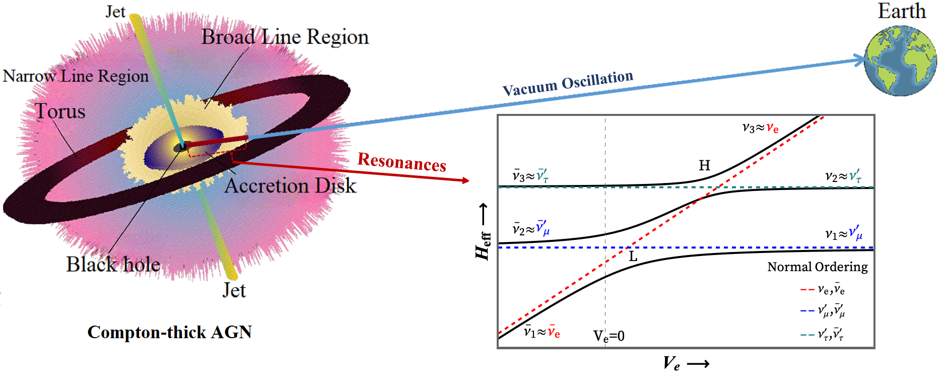
Figure 1: Schematic illustration of neutrino propagation in AGNs. Neutrinos are produced close to the central BH (accretion disk and BLR), where densities are very high and ME are important. As a consequence, neutrinos undergo MSW conversions ($H$ and $L$-resonances) before they reach the vacuum and propagate to the Earth. Also shown are the energy levels of a neutrino system propagating in a slowly decreasing density profile. See main text and Appendix for details.

Neutrino production in AGNs.– AGNs are natural particle accelerators where neutrinos are created via collision of accelerated protons ($pp$) or by photohadronic interactions of protons with $\gamma$-rays in the environment ($p\gamma$) [29, 30, 31, 32, 33]. Both $pp$ and $p\gamma$ interactions produce high-energy pions that subsequently decay to neutrinos, $\pi^{\pm}\rightarrow\mu^{\pm}+\nu_{\mu}/\bar{\nu}_{\mu}\rightarrow e^{\pm}+\bar{\nu_{e}}/\nu_{e}+\nu_{\mu}+\bar{\nu}_{\mu}$, with source flavor ratio $(f_{\nu_{e}+\bar{\nu}_{e}},f_{\nu_{\mu}+\bar{\nu}_{\mu}},f_{\nu_{\tau}+\bar{\nu}_{\tau}})_{S}=(1,2,0)_{S}$ which then propagate vast cosmic distances to reach the Earth. It is usually assumed that due to VO, neutrino fluxes at Earth are shared equally among the three flavors: $(f_{\nu_{e}+\bar{\nu}_{e}},f_{\nu_{\mu}+\bar{\nu}_{\mu}},f_{\nu_{\tau}+\bar{\nu}_{\tau}})_{\oplus}=(1,1,1)_{\oplus}$ [44], as predicted by the measured structure of the mixing matrix [63, 64, 65]. Deviations from the total flavor equipartition are possible. For instance, if the muon from the pion decay rapidly loses energy due to environmental interactions (e.g. synchrotron emission) before decaying (muon-damped case) [66, 67, 68, 69, 70], the produced flavor ratio is $(0,1,0)_{S}$ which translates to $(4,12,9)_{\oplus}$. Analogously, if the source somehow injects a nearly pure neutron flux [71, 72], the source flavor ratio is $(1,0,0)_{S}$, which translates to $(14,4,7)_{\oplus}$.

Influence of AGN matter.– The main point of this work is that neutrino flavor conversion is necessarily affected by the high matter densities encountered in the AGN cores where neutrinos are produced. We specifically focus on obscured AGNs [34], where neutrinos are produced in the vicinity of the central BH, at radial distances of 10–100 Schwarzschild radii ($R_{s}$) [73, 42, 33] and go through regions filled with relatively dense gas such as the upper layers of the BH accretion disk, the Broad Line Region (BLR) and the torus, see Fig. 1. To give a sense of the scales involved here, the host galaxy is roughly 1 kpc across, the inner (outer) radius of the torus is about 1 (10) pc from the center, and neutrinos are produced close to the accretion disk, $\sim 10^{-5}$ pc from the central region, equivalent to $10R_{s}$ for a black hole of mass $10^{7}M_{\odot}$ [42]. In the accretion disk and inner parts of BLR, particle number densities were inferred to reach up to $10^{21}\,{\rm cm}^{-3}$ [74, 75, 76]. In the outer parts of the BLR, where it meets the torus, densities drop to $10^{11}\,\text{cm}^{-3}$ [77, 78]. Hence, we deduce that the neutrinos can undergo Mikheyev-Smirnov-Wolfenstein (MSW) resonant flavor conversion [79, 80, 81, 82] on their way out from the AGN as the matter density decreases from the inner to the outer BLR region and the resonance criteria are met.

BLR geometry and density profile.– The BLR geometry is assumed to be either a flared disk-shaped or spherical region formed by gas that is bounded by the gravitational influence of the central BH, and emits optical/UV broad emission lines [83, 84, 85, 86, 87]. It extends from the upper accretion disk up to the inner edge of the torus. The BLR is usually depicted in the literature as made out of discrete clouds. Nevertheless, the number of clouds can be so high that the gas can be treated as homogeneous [86]. We describe the BLR electron number density with a power law [77, 78]:

$$n_{e}(r)=(10^{11}\,\text{cm}^{-3})\left(\frac{1~{}\text{pc}}{r}\right)^{2},$$ (1)

normalized to have $n_{e}=10^{11}\,\text{cm}^{-3}$ at the inner edge of the BLR ($r=1$ pc) and $n_{e}=10^{21}\,\text{cm}^{-3}$ in upper accretion disk ($r=10^{-5}$ pc). We assume that Eq. (1) is valid for $r\gtrsim 10^{-5}$ pc ($r\gtrsim 10R_{s}$ for a BH mass $10^{7}M_{\odot}$, such as in NGC 1068 [42]) so that the profile describes the whole range of densities from where neutrinos are produced to the end of the BLR. We comment on the consequences of modifying certain assumptions in Eq. (1) in the next sections.

Evolution Hamiltonian.– Neutrino flavor evolution can be described by the Schrödinger equation

$$i\frac{d}{dr}\nu=\mathcal{H}_{\rm eff}\nu,$$ (2)

where $\nu=(\nu_{e},\nu_{\mu},\nu_{\tau})^{T}$ is the flavor state, $r$ is the radial coordinate in a system that has the BH in the center with neutrinos traveling outwards through the BLR (Fig. 1) and $\mathcal{H}_{\rm eff}$ is the effective flavor Hamiltonian in presence of matter:

$$\mathcal{H}_{\rm eff}=\frac{1}{2E}U\left(\begin{array}[]{ccc}0&0&0\\ 0&\Delta m_{21}^{2}&0\\ 0&0&\Delta m_{31}^{2}\end{array}\right)U^{\dagger}+V_{e}\left(\begin{array}[]{ccc}1&0&0\\ 0&0&0\\ 0&0&0\end{array}\right).$$ (3)

The first term on the right-hand side governs VO. The PMNS matrix, $U$, is parametrized in terms of the three mixing angles $\theta_{ij}$, $\Delta m_{j1}^{2}$’s are the mass-square differences, and $E$ is the energy [88]. The second term contains the matter potential $V_{e}(r)=\sqrt{2}G_{F}n_{e}(r)$, where $G_{F}$ is the Fermi constant, that affects only electron neutrinos via charged-current weak interaction $\nu_{e}+e^{-}\rightarrow\nu_{e}+e^{-}$ [79]. Neutral-current interactions give the same contributions to all flavors and do not impact the flavor conversion. For antineutrinos, the only difference is the sign of the matter potential ($V_{e}\rightarrow-V_{e}$).

Flavor conversion.– Neutrino flavor conversion in a varying density profile such as Eq. (1) can happen at the high ($H$) and low ($L$) resonant layers [89]. The average number density, $n_{e}^{\rm res}$, corresponding to both resonant layers is given by

$$\sqrt{2}G_{F}n_{e}^{\rm res}=\frac{\Delta m^{2}_{i1}}{2E}\cos 2\theta_{1i},$$ (4)

where $L$ ($H$) corresponds to $i=2$ (3). Eq. (4) is derived in the two-flavor approximation but is valid for the three-flavor system in Eq. (3), provided the resonant layers factorize and act independently [89]. Numerically, $n_{e}^{H}\approx 10^{20}\text{cm}^{-3}(100\text{ TeV}/E)$ and $n_{e}^{L}\approx 10^{18}\text{cm}^{-3}(100\text{ TeV}/E)$, with the oscillation parameters taken from Ref. [63]. In addition, we can estimate the width of the resonant layer as $\Delta n_{e}^{\rm res}\approx n_{e}^{\rm res}\tan 2\theta_{1i}$ [82]. It is necessary that neutrinos cross the entire resonant layer adiabatically for efficient conversion. The level of adiabaticity of the resonant layer is measured by

$$\gamma=\frac{\Delta m^{2}_{i1}\sin^{2}2\theta_{1i}}{2E\cos 2\theta_{1i}}\left(\frac{1}{n_{e}^{\rm res}}\left|\frac{dn_{e}}{dr}\right|_{\rm res}\right)^{-1},$$ (5)

and $\gamma>1$ means adiabatic propagation [89].

If we assume the profile in Eq. (1) and neutrinos are produced at $10R_{s}\sim 10^{-5}$ pc, then both resonance densities are met during propagation for $E>10$ TeV as $n_{e}(10^{-5}\ \text{pc})\simeq 10^{21}\text{cm}^{-3}>n_{e}^{H}$ (and obviously $n_{e}^{L}$) at these energies. Nevertheless, the $H$-resonance starts to be effective only for $E>70$ TeV, as $n^{H}_{e}$ falls below $10^{20}\,\text{cm}^{-3}$ and neutrinos produced at $n_{e}\approx 10^{21}\,\text{cm}^{-3}$ have the chance to cross the entire resonant layer. The upper limit on the effectiveness of the $H$-resonance is at $\sim 1$ PeV due to $\gamma$, in Eq. (5), falling below $1$ for higher energies. The $L$-resonance, on the contrary, is effective even for energies down to $1$ TeV and up until $100$ PeV, thus covering the entire HEN spectrum observed by IceCube [10].

We can modify Eq. (1) in two simple ways, either by changing its normalization or its power-law index. By decreasing any of these parameters, we reduce densities close to the BH, and the $H$-resonance cannot be met. Nevertheless, the $L$-resonance alone can still generate flavor conversion, even for initial densities of order $10^{18}\,\text{cm}^{-3}$. If we increase the power-law index, both resonances are achieved, but the $H$-resonance cannot be adiabatic for power-law index $\gtrsim 3$ due to fast variation of the profile, see Eq. (5). The $L$-resonance, on the other hand, remains adiabatic in the range $100$ TeV to $1$ PeV and is a robust spot for flavor conversion even in the absence of the $H$-resonance.

Results.– In the absence of ME during propagation, the initial flavor content is modified by averaged-out VO. The probability that an initial flavor $\nu_{\alpha}$ will change to a flavor $\nu_{\beta}$ on its way to the Earth is given by [90, 91]

$$P_{\alpha\beta}^{\mathrm{VO}}=\sum_{i=1}^{3}\left|U_{\alpha i}\right|^{2}\left|U_{\beta i}\right|^{2},$$ (6)

where $U_{\alpha i}$ are the PMNS matrix elements. For an initial flavor composition $(f_{e}^{S},f_{\mu}^{S},f_{\tau}^{S})$ at the source ($S$), the composition that reaches the Earth is

$$f_{\beta}^{\oplus}=\sum_{\alpha=e,\mu,\tau}P_{\alpha\beta}^{\mathrm{VO}}f_{\alpha}^{S}\,.$$ (7)

Therefore, for VO without any ME, the flavor content for different production channels changes along propagation as (applicable for both $pp$ and $p\gamma$ sources)

$$\pi \hskip 14.22636pt(1/3,2/3,0)_{S}\rightarrow(0.3,0.37,0.33)_{\oplus},$$-decay:

$$\mu \hskip 14.22636pt(0,1,0)_{S}\rightarrow(0.17,0.47,0.36)_{\oplus},$$-damped:

$$n \hskip 14.22636pt(1,0,0)_{S}\rightarrow(0.55,0.17,0.28)_{\oplus},$$-decay: (8)

using the best-fit values of the oscillation parameters [63], as shown by the colored circles on the left panel of Fig. 2. Taking into account the $3\sigma$ interval of the parameters [63], we get the colored regions in Fig. 2. Results in the main text are shown for NO, while plots for IO, which are very similar to NO for VO, are given in the Appendix (Fig. 3). Similar flavor triangle analyses in the VO case have been done before [92, 93, 94, 95, 96, 97, 98].

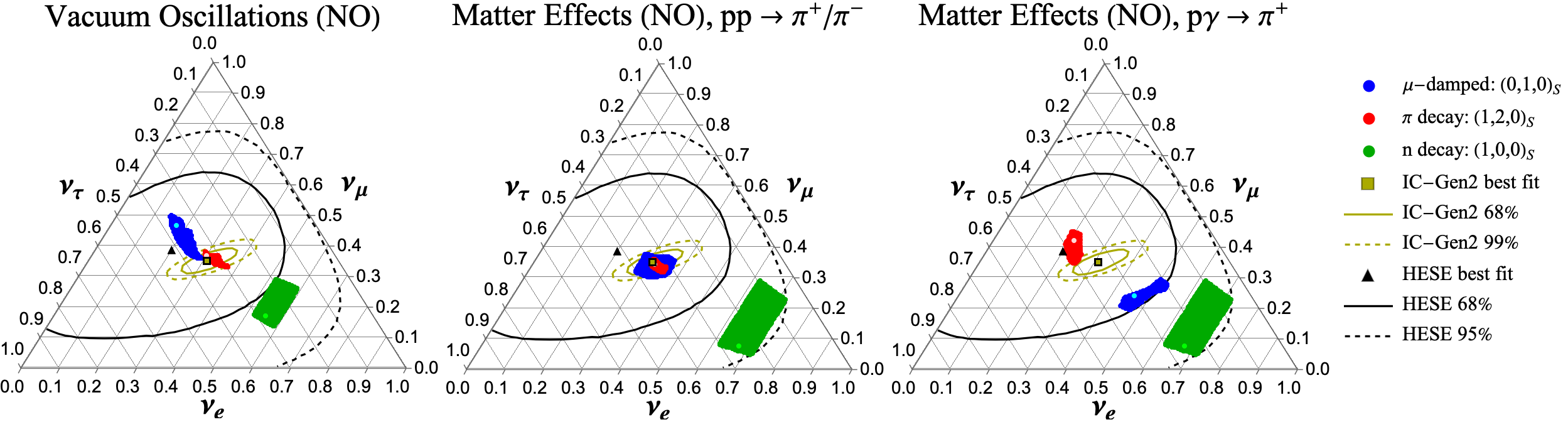
Figure 2: Left: Allowed regions of flavor ratios of astrophysical neutrinos on Earth after accounting for vacuum oscillations en route and the $3\sigma$ neutrino oscillation parameters (assuming normal ordering) from a recent global fit [63]. Middle: Same regions after the inclusion of ME at the source and assuming $pp$ production. Right: Regions are further modified if instead we assume $p\gamma$ production in combination with ME. In each panel, we consider 3 scenarios: standard pion decay (red), muon-damped (blue) and neutron decay (green). Also shown are the current IceCube constraints (black solid and dashed for 68% and 95% C.L. respectively) [9] and projections for IceCube-Gen2 (yellow) [46].

Our main new result is that ME can substantially modify the allowed regions for flavor ratios observed on Earth. First of all, different from VO, ME can distinguish neutrinos from antineutrinos and between production processes that are asymmetrical between them, such as $pp$ and $p\gamma$, see Fig. 2 middle and right panels. The $pp$ interactions produce roughly equal ratios of $\pi^{+}$ and $\pi^{-}$ [91, 61] and, therefore, $\nu_{e}$ and $\bar{\nu}_{e}$ are created in equal amounts. On the other hand, $p\gamma$ suppresses the production $\pi^{-}$ relative to that of $\pi^{+}$, and hence, mostly $\nu_{e}$’s are created. Equal amounts of $\nu_{\mu}$ and $\bar{\nu}_{\mu}$ are created in both processes.

Here, we describe the pattern of flavor conversion via $H$ and $L$-resonances in the central parts of AGNs using the energy level diagram in Fig. 1 and assuming both layers to be perfectly adiabatic (see a discussion on the energy level diagram in the Appendix). We start with $\nu_{e}$ ($\bar{\nu}_{e}$), produced in dense matter as $\nu_{3}^{m}$ ($\nu_{1}^{m}$), which reaches vacuum as $\nu_{3}$ ($\nu_{1}$):

$$\text{For $\nu_{e}$:}\hskip 14.22636pt(1,0,0)_{S}^{\nu} \rightarrow\left(\left|U_{e3}\right|^{2},\left|U_{\mu 3}\right|^{2},\left|U_{\tau 3}\right|^{2}\right)_{\oplus}^{\nu}$$

$$=(0.02,0.56,0.42)_{\oplus}^{\nu}.$$ (9)

$$\text{For $\bar{\nu}_{e}$:}\hskip 14.22636pt(1,0,0)_{S}^{\bar{\nu}} \rightarrow\left(\left|U_{e1}\right|^{2},\left|U_{\mu 1}\right|^{2},\left|U_{\tau 1}\right|^{2}\right)_{\oplus}^{\bar{\nu}}$$

$$=(0.67,0.08,0.25)_{\oplus}^{\bar{\nu}}.$$ (10)

The superscript $\nu$ and $\bar{\nu}$ indicate that a given flavor is populated only by neutrinos or antineutrinos, respectively. Following the discussion on energy levels, $\nu_{\mu}$ ($\bar{\nu}_{\mu}$) reaches vacuum as incoherent mixtures of $\nu_{1}$ and $\nu_{2}$ ($\nu_{2}$ and $\nu_{3}$), therefore:

$$\text{For $\nu_{\mu}$:}\hskip 14.22636pt(0,1,0)_{S}^{\nu}\rightarrow$$

$$\frac{1}{2}\left(\left|U_{e1}\right|^{2}+\left|U_{e2}\right|^{2},\left|U_{\mu 1}\right|^{2}+\left|U_{\mu 2}\right|^{2},\left|U_{\tau 1}\right|^{2}+\left|U_{\tau 2}\right|^{2}\right)_{\oplus}^{\nu}$$

$$\qquad\qquad=(0.5,0.2,0.3)_{\oplus}^{\nu}.$$ (11)

$$\text{For $\bar{\nu}_{\mu}$:}\hskip 14.22636pt(0,1,0)_{S}^{\bar{\nu}}\rightarrow$$

$$\frac{1}{2}\left(\left|U_{e2}\right|^{2}+\left|U_{e3}\right|^{2},\left|U_{\mu 2}\right|^{2}+\left|U_{\mu 3}\right|^{2},\left|U_{\tau 2}\right|^{2}+\left|U_{\tau 3}\right|^{2}\right)_{\oplus}^{\bar{\nu}}$$

$$\qquad\qquad=(0.17,0.46,0.37)_{\oplus}^{\bar{\nu}}.$$ (12)

With Eqs. (9)-(12) we can estimate the results for all relevant production processes of HENs in AGNs, taking ME into account. For $pp$ process, total $\pi^{+}/\pi^{-}$ decay leads to the proportion $\frac{1}{6}\nu_{e}+\frac{1}{6}\bar{\nu}_{e}+\frac{1}{3}\nu_{\mu}+\frac{1}{3}\bar{\nu}_{\mu}$, while for $\mu$-damped, we have $\frac{1}{2}\nu_{\mu}+\frac{1}{2}\bar{\nu}_{\mu}$. Therefore,

$$\pi pp \hskip 14.22636pt(1/3,2/3,0)_{S}\rightarrow(0.34,0.33,0.33)_{\oplus}.$$-decay ():

$$\mu pp \hskip 14.22636pt(0,1,0)_{S}\rightarrow(0.34,0.33,0.33)_{\oplus}.$$-damped (): (13)

Contrary to VO case, for ME and $pp$ production, the $\pi$-decay and $\mu$-damped processes cannot be disentangled, see Fig. 2 (middle panel).

For $p\gamma$ case, only $\pi^{+}$ is produced from $\Delta^{+}$ resonance and decays in the proportion $\frac{1}{3}\nu_{e}+\frac{1}{3}\nu_{\mu}+\frac{1}{3}\bar{\nu}_{\mu}$, while $\mu$-damped creates only $\nu_{\mu}$. Then,

$$\pi p\gamma \hskip 14.22636pt(1/3,2/3,0)_{S}\rightarrow(0.23,0.4,0.37)_{\oplus}.$$-decay ():

$$\mu p\gamma \hskip 14.22636pt(0,1,0)_{S}\rightarrow(0.5,0.2,0.3)_{\oplus}.$$-damped (): (14)

In this case, both $\pi$-decay and $\mu$-damped are completely displaced from their VO expected regions in the flavor triangle, see Fig. 2 (right panel). In particular, $\mu$-damped and ME can be confused with $n$-decay and VO, while $\pi$-decay and ME can be confused with $\mu$-damped and VO.

For both processes,

$$n pp p\gamma ~{}(1,0,0)_{S}\rightarrow(0.67,0.08,0.25)_{\oplus}.$$-decay ( & ): (15)

The allowed region corresponding to $n$-decay is also displaced to the lower right vertex on the flavor triangle when compared to the pure VO case. The most impressive change in the $n$-decay allowed region comes in IO, see Appendix. We summarize the best-fit NO results in Table 1.

Vacuum Oscillations (NO)
$\pi$-decay	$\hskip 14.22636pt(1/3,2/3,0)_{S}\rightarrow(0.30,0.37,0.33)_{\oplus}\hskip 14.22636pt$
$\mu$-damped	$\hskip 14.22636pt(0,1,0)_{S}\rightarrow(0.17,0.47,0.36)_{\oplus}\hskip 14.22636pt$
$n$-decay	$\hskip 14.22636pt(1,0,0)_{S}\rightarrow(0.55,0.17,0.28)_{\oplus}\hskip 14.22636pt$

Matter Effect (NO), $pp$ production
$\pi$-decay	$\hskip 14.22636pt(1/3,2/3,0)_{S}\rightarrow(0.34,0.33,0.33)_{\oplus}\hskip 14.22636pt$
$\mu$-damped	$\hskip 14.22636pt(0,1,0)_{S}\rightarrow(0.34,0.33,0.33)_{\oplus}\hskip 14.22636pt$
$n$-decay	$\hskip 14.22636pt(1,0,0)_{S}\rightarrow(0.67,0.08,0.25)_{\oplus}\hskip 14.22636pt$

Matter Effect (NO), $p\gamma$ production
$\pi$-decay	$\hskip 14.22636pt(1/3,2/3,0)_{S}\rightarrow(0.23,0.40,0.37)_{\oplus}\hskip 14.22636pt$
$\mu$-damped	$\hskip 14.22636pt(0,1,0)_{S}\rightarrow(0.50,0.20,0.30)_{\oplus}\hskip 14.22636pt$
$n$-decay	$\hskip 14.22636pt(1,0,0)_{S}\rightarrow(0.67,0.08,0.25)_{\oplus}\hskip 14.22636pt$

Table 1: Summary of our flavor conversion results, assuming normal mass ordering.

Fig. 2 also includes the $68\%$ and $95\%$ C.L. bounds on the flavor composition of the diffuse HEN flux from the IceCube analysis [9] using the High-Energy Starting Events (HESE) sample [8], which is an all-sky and all-flavor search with neutrinos above $60$ TeV, collected during 7.5 years of IceCube lifetime. Observe that while the $95\%$ C.L. region is compatible with all possible flavor compositions, the current best fit is closer to $\mu$-damped region for VO. After including ME and assuming dominant AGN contribution to the HEN flux [24], the best fit can be explained by a pure $\pi$-decay after $p\gamma$ production, see Fig. 2. In this last scenario, all other production processes are partially outside of the $68\%$ C.L., although they can be relevant in combination with $\pi$-decay. Nevertheless, more statistics is necessary to further constrain the flavor ratios, see, for example, the preliminary analysis in Ref. [45]. Future detectors will also improve our understanding of the flavor composition in the next decades [98]. In Fig. 2, we include projections from IceCube-Gen2 after $10$ years of operations (yellow contours) assuming $\pi$-decay and VO to be the true hypothesis [46].

Neutrino flavor conversion in AGNs can also be directly studied by using single sources. The increasing evidence for neutrinos pointing to steady-state AGN sources can allow for individual studies of flavor composition in different energy regimes. In the Appendix, we complement the discussion by including the flavor triangles for IO, which can be completely different from NO, due to differences in the energy level scheme.

Discussion and Conclusions.– The AGN model used in Eq. (1) has a column density $N_{\rm H}\equiv\int n_{e}dr\sim 10^{33}\,\text{cm}^{-2}$, compatible with the minimum necessary width of the medium for strong flavor conversion [43]. Flavor conversion via the $L$-resonance alone can be achieved at smaller $N_{\rm H}\sim 10^{30}\,\text{cm}^{-2}$, which is still orders of magnitude higher than that ($\sim 10^{25}\,\text{cm}^{-2}$) inferred for NGC 1068 from $X$-ray studies [99, 100]. Such heavily Compton-thick AGNs, with $N_{\rm H}\geq\sigma_{T}^{-1}\simeq 1.5\times 10^{24}\,\text{cm}^{-2}$ (inverse of the Thomson cross-section, which corresponds to unity optical depth for Compton scattering), could be numerous [101, 102, 38], but detecting them is challenging by conventional astrophysical methods due to $X$-ray absorption [103, 104, 34]. HENs, unaffected by obscuration, offer an exciting multi-messenger avenue to study these AGNs, complementary to searches based on infrared emission and star formation. Our proposed mechanism, measuring a shift in the flavor ratios influenced by ME, provides a unique probe of the Compton-thick AGNs as the sources of the HESE neutrinos. Understanding the distribution of Compton-thick AGNs is also crucial for modeling their impact on the cosmic $X$-ray background and gaining insights into the correlation between black hole growth and galaxy evolution [105].

The analysis performed here assumes that the flavor composition at Earth is constant over the observed neutrino energy range. The capability of future neutrino telescopes to do such energy-dependent measurements, i.e., to look for a transition from neutrino production via the full pion decay chain at low energies to muon-damped pion decay at high energies, was recently assessed in Ref. [106]. Taking into account the ME discussed here can modify the energy dependence of the flavor ratios in a nontrivial way. This will be studied in a follow-up work.

We have examined the resonant flavor conversion of HENs within the standard 3-neutrino oscillation paradigm. Additional new physics phenomena, such as Glashow-like resonances in neutrino mass models [107, 108], spin-flavor resonance for transition magnetic moments of Majorana neutrinos [109], or spin-flip resonance of Dirac neutrinos [110], could impact the source flavor ratios as well. In general, the presence of new physics is known to complicate the flavor triangle analysis [111, 112, 113, 114, 115, 116, 117, 118, 119, 120, 121]. Exploring the ME in presence of other new physics effects is beyond the scope of this study and will be addressed in future research.

Acknowledgments.– We thank Manel Errando and Alexei Smirnov for useful discussions. The work of BD was partly supported by the U.S. Department of Energy under grant No. DE-SC 0017987. The work of YP was supported in part by the São Paulo Research Foundation (FAPESP) Grant No. 2023/10734-3. We thank the Fermilab Theoretical Physics Department, where part of this work was done, for their warm hospitality. BD and SJ also wish to acknowledge the Center for Theoretical Underground Physics and Related Areas (CETUP*) and the Institute for Underground Science at SURF for hospitality and for providing a stimulating environment.

Appendix

Energy levels.– Here, we discuss the energy levels of the Hamiltonian in Eq. (3), which we show in Fig. 1 for normal ordering (NO). For illustrative purposes, these energy levels are plotted for fictitious values of $\Delta m^{2}_{21}$ and $\Delta m^{2}_{31}$ ($7$ $\text{eV}^{2}$ and $15$ $\text{eV}^{2}$, respectively) while the mixing angles are chosen close to their best-fit values ($\theta_{12}=34^{\circ}$, $\theta_{13}=8^{\circ}$, $\theta_{23}=45^{\circ}$).

Firstly, recall from the previous discussion that we can represent antineutrinos as neutrinos with negative $V_{e}$. At very high densities, or large $|V_{e}|$, $|\mathcal{H}_{ee}|$ is much larger than the mixing terms in $\mathcal{H}$ and $\nu_{e}$ ($\bar{\nu}_{e}$) becomes the heaviest (lightest) matter eigenstate. Meanwhile, the other eigenstates are roughly an equal mixture ($\theta_{23}\sim 45^{o}$) of $\nu_{\mu}$ and $\nu_{\tau}$; we denote them as $\nu^{\prime}_{\mu}$ and $\nu^{\prime}_{\tau}$. As $\mathcal{H}_{ee}$ is linear in $V_{ee}$, for $\nu_{e}$ ($\bar{\nu}_{e}$) produced at high densities ($\gg n_{H}^{\rm res},n_{L}^{\rm res}$), their energy levels can cross the levels of $\nu^{\prime}_{\mu}$ and $\nu^{\prime}_{\tau}$ (and antineutrinos) as they propagate towards vacuum densities ($\ll n_{H}^{\rm res},n_{L}^{\rm res}$). At these crossings, the $H$ and $L$-resonances occur [89]. For NO, both resonances happen for neutrinos. For IO, the $H$-resonance moves to the antineutrino channel. While the levels of the flavor state cross, the levels of matter eigenstates ($\nu_{3}^{m}$, $\nu_{2}^{m}$, and $\nu_{1}^{m}$) do not. Therefore, the eigenstates in matter exchange flavor content at resonances and lead the system to flavor conversion.

The flavor triangle analysis, including the ME for the IO scenario, is shown in Fig. 3, and summarized in Table 2. Finally, Figs. 4 and 5 show the results for NO and IO, respectively, for the case where only the $L$-resonance is effective.

Vacuum Oscillations (IO)
$\pi$-decay	$\hskip 14.22636pt(1/3,2/3,0)_{S}\rightarrow(0.32,0.35,0.33)_{\oplus}\hskip 14.22636pt$
$\mu$-damped	$\hskip 14.22636pt(0,1,0)_{S}\rightarrow(0.20,0.42,0.38)_{\oplus}\hskip 14.22636pt$
$n$-decay	$\hskip 14.22636pt(1,0,0)_{S}\rightarrow(0.55,0.20,0.25)_{\oplus}\hskip 14.22636pt$

Matter Effect (IO), $pp$ production
$\pi$-decay	$\hskip 14.22636pt(1/3,2/3,0)_{S}\rightarrow(0.33,0.33,0.34)_{\oplus}\hskip 14.22636pt$
$\mu$-damped	$\hskip 14.22636pt(0,1,0)_{S}\rightarrow(0.42,0.28,0.30)_{\oplus}\hskip 14.22636pt$
$n$-decay	$\hskip 14.22636pt(1,0,0)_{S}\rightarrow(0.02,0.56,0.42)_{\oplus}\hskip 14.22636pt$

Matter Effect (IO), $p\gamma$ production
$\pi$-decay	$\hskip 14.22636pt(1/3,2/3,0)_{S}\rightarrow(0.38,0.28,0.34)_{\oplus}\hskip 14.22636pt$
$\mu$-damped	$\hskip 14.22636pt(0,1,0)_{S}\rightarrow(0.34,0.36,0.30)_{\oplus}\hskip 14.22636pt$
$n$-decay	$\hskip 14.22636pt(1,0,0)_{S}\rightarrow(0.02,0.56,0.42)_{\oplus}\hskip 14.22636pt$

Table 2: Summary of our flavor conversion results, assuming inverted mass ordering.

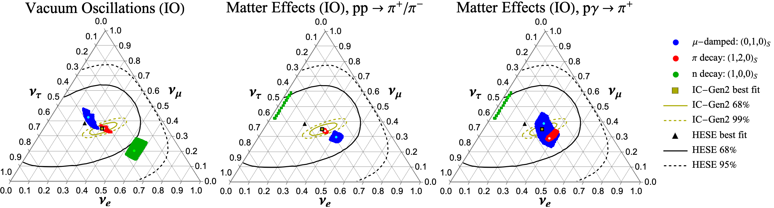
Figure 3: Same as Fig. 2 but for inverted ordering (IO).

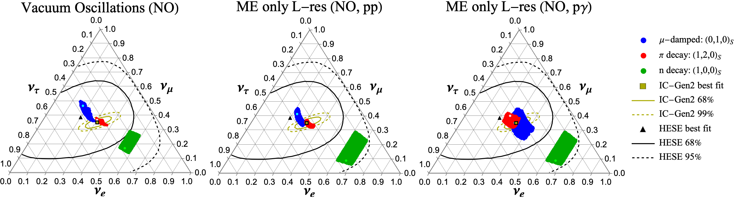
Figure 4: Same as Fig. 2 (NO) but assuming that only the $L$-resonance is effective.

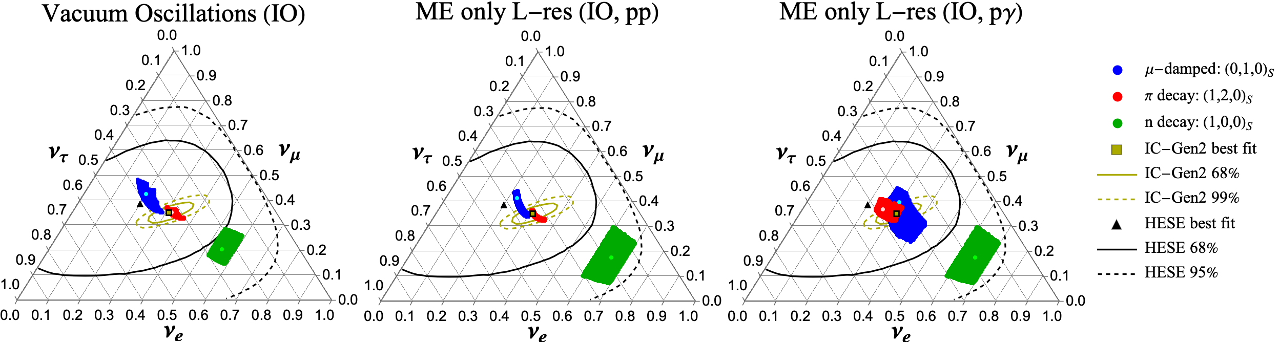
Figure 5: Same as Fig. 3 (IO) but assuming that only the $L$-resonance is effective.

References

- [1] IceCube, M. G. Aartsen et al., “First observation of PeV-energy neutrinos with IceCube,” Phys. Rev. Lett. 111 (2013) 021103, arXiv:1304.5356.
- [2] IceCube, M. G. Aartsen et al., “Evidence for High-Energy Extraterrestrial Neutrinos at the IceCube Detector,” Science 342 (2013) 1242856, arXiv:1311.5238.
- [3] M. Ahlers and F. Halzen, “Opening a New Window onto the Universe with IceCube,” Prog. Part. Nucl. Phys. 102 (2018) 73–88, arXiv:1805.11112.
- [4] IceCube, M. G. Aartsen et al., “Observation of High-Energy Astrophysical Neutrinos in Three Years of IceCube Data,” Phys. Rev. Lett. 113 (2014) 101101, arXiv:1405.5303.
- [5] IceCube, M. G. Aartsen et al., “A combined maximum-likelihood analysis of the high-energy astrophysical neutrino flux measured with IceCube,” Astrophys. J. 809 (2015) no. 1, 98, arXiv:1507.03991.
- [6] IceCube, M. G. Aartsen et al., “Evidence for Astrophysical Muon Neutrinos from the Northern Sky with IceCube,” Phys. Rev. Lett. 115 (2015) no. 8, 081102, arXiv:1507.04005.
- [7] IceCube, M. G. Aartsen et al., “Observation and Characterization of a Cosmic Muon Neutrino Flux from the Northern Hemisphere using six years of IceCube data,” Astrophys. J. 833 (2016) no. 1, 3, arXiv:1607.08006.
- [8] IceCube, R. Abbasi et al., “The IceCube high-energy starting event sample: Description and flux characterization with 7.5 years of data,” Phys. Rev. D 104 (2021) 022002, arXiv:2011.03545.
- [9] IceCube, R. Abbasi et al., “Detection of astrophysical tau neutrino candidates in IceCube,” Eur. Phys. J. C 82 (2022) no. 11, 1031, arXiv:2011.03561.
- [10] IceCube, R. Abbasi et al., “Improved Characterization of the Astrophysical Muon–neutrino Flux with 9.5 Years of IceCube Data,” Astrophys. J. 928 (2022) no. 1, 50, arXiv:2111.10299.
- [11] ANTARES, A. Albert et al., “All-flavor Search for a Diffuse Flux of Cosmic Neutrinos with Nine Years of ANTARES Data,” Astrophys. J. Lett. 853 (2018) no. 1, L7, arXiv:1711.07212.
- [12] Baikal-GVD, V. A. Allakhverdyan et al., “Diffuse neutrino flux measurements with the Baikal-GVD neutrino telescope,” Phys. Rev. D 107 (2023) no. 4, 042005, arXiv:2211.09447.
- [13] N. Kurahashi, K. Murase, and M. Santander, “High-Energy Extragalactic Neutrino Astrophysics,” Ann. Rev. Nucl. Part. Sci. 72 (2022) 365, arXiv:2203.11936.
- [14] S. Troitsky, “The origin of high-energy astrophysical neutrinos: new results and prospects,” arXiv:2311.00281.
- [15] M. Ahlers, Y. Bai, V. Barger, and R. Lu, “Galactic neutrinos in the TeV to PeV range,” Phys. Rev. D 93 (2016) no. 1, 013009, arXiv:1505.03156.
- [16] IceCube, R. Abbasi et al., “Observation of high-energy neutrinos from the Galactic plane,” Science 380 (2023) no. 6652, adc9818, arXiv:2307.04427.
- [17] F. S. Greus and A. S. Losa, “Multimessenger Astronomy with Neutrinos,” Universe 7 (2021) no. 11, 397, arXiv:2110.11817.
- [18] C. Guépin, K. Kotera, and F. Oikonomou, “High-energy neutrino transients and the future of multi-messenger astronomy,” Nature Rev. Phys. 4 (2022) no. 11, 697–712, arXiv:2207.12205.
- [19] IceCube, M. G. Aartsen et al., “Neutrino emission from the direction of the blazar TXS 0506+056 prior to the IceCube-170922A alert,” Science 361 (2018) no. 6398, 147–151, arXiv:1807.08794.
- [20] M. G. Aartsen et al., “Multimessenger observations of a flaring blazar coincident with high-energy neutrino IceCube-170922A,” Science 361 (2018) no. 6398, eaat1378, arXiv:1807.08816.
- [21] X. Rodrigues, S. Garrappa, S. Gao, V. S. Paliya, A. Franckowiak, and W. Winter, “Multiwavelength and Neutrino Emission from Blazar PKS 1502 + 106,” Astrophys. J. 912 (2021) no. 1, 54, arXiv:2009.04026.
- [22] IceCube, R. Abbasi et al., “Evidence for neutrino emission from the nearby active galaxy NGC 1068,” Science 378 (2022) no. 6619, 538–543, arXiv:2211.09972.
- [23] ANTARES, OVRO, A. Albert et al., “Searches for neutrinos in the direction of radio-bright blazars with the ANTARES telescope,” arXiv:2309.06874.
- [24] IceCube, R. Abbasi et al., “Search for neutrino emission from cores of active galactic nuclei,” Phys. Rev. D 106 (2022) no. 2, 022005, arXiv:2111.10169.
- [25] K. Murase and F. W. Stecker, “Chapter 10: High-Energy Neutrinos from Active Galactic Nuclei,” arXiv:2202.03381.
- [26] R. Antonucci, “Unified models for active galactic nuclei and quasars,” Ann. Rev. Astron. Astrophys. 31 (1993) 473–521.
- [27] C. M. Urry and P. Padovani, “Unified schemes for radio-loud active galactic nuclei,” Publ. Astron. Soc. Pac. 107 (1995) 803, arXiv:astro-ph/9506063.
- [28] IceCube, M. G. Aartsen et al., “The contribution of Fermi-2LAC blazars to the diffuse TeV-PeV neutrino flux,” Astrophys. J. 835 (2017) no. 1, 45, arXiv:1611.03874.
- [29] K. Murase, D. Guetta, and M. Ahlers, “Hidden Cosmic-Ray Accelerators as an Origin of TeV-PeV Cosmic Neutrinos,” Phys. Rev. Lett. 116 (2016) no. 7, 071101, arXiv:1509.00805.
- [30] K. Murase, S. S. Kimura, and P. Meszaros, “Hidden Cores of Active Galactic Nuclei as the Origin of Medium-Energy Neutrinos: Critical Tests with the MeV Gamma-Ray Connection,” Phys. Rev. Lett. 125 (2020) no. 1, 011101, arXiv:1904.04226.
- [31] S. Inoue, M. Cerruti, K. Murase, and R.-Y. Liu, “Multimessenger emission from winds and tori in active galactic nuclei,” PoS ICRC2023 (2023) 1161, arXiv:2207.02097.
- [32] K. Fang, J. S. Gallagher, and F. Halzen, “The TeV Diffuse Cosmic Neutrino Spectrum and the Nature of Astrophysical Neutrino Sources,” Astrophys. J. 933 (2022) no. 2, 190, arXiv:2205.03740.
- [33] F. Halzen, “IceCube: Neutrinos from Active Galaxies,” in 57th Rencontres de Moriond on Electroweak Interactions and Unified Theories. 5, 2023. arXiv:2305.07086.
- [34] R. C. Hickox and D. M. Alexander, “Obscured Active Galactic Nuclei,” Ann. Rev. Astron. Astrophys. 56 (2018) 625–671, arXiv:1806.04680.
- [35] Fermi-LAT, S. Abdollahi et al., “A gamma-ray determination of the Universe’s star formation history,” Science 362 (2018) no. 6418, 1031–1034, arXiv:1812.01031.
- [36] J. Li et al., “Piercing Through Highly Obscured and Compton-thick AGNs in the Chandra Deep Fields: I. X-ray Spectral and Long-term Variability Analyses,” Astrophys. J. 877 (2019) no. 1, 5, arXiv:1904.03827.
- [37] E. L. Lambrides, M. Chiaberge, T. Heckman, R. Gilli, F. Vito, and C. Norman, “A Large Population of Obscured AGN in Disguise as Low-luminosity AGN in Chandra Deep Field South,” Astrophys. J. 897 (2020) no. 2, 160, arXiv:2002.00955.
- [38] C. M. Carroll, T. T. Ananna, R. C. Hickox, A. Masini, R. J. Assef, D. Stern, C.-T. J. Chen, and L. Lanz, “A High Fraction of Heavily X-Ray-obscured Active Galactic Nuclei,” Astrophys. J. 950 (2023) no. 2, 127, arXiv:2303.08813.
- [39] W. Yan et al., “The Most Obscured AGNs in the XMM-SERVS Fields,” Astrophys. J. 951 (2023) no. 1, 27, arXiv:2304.06065.
- [40] M. Signorini et al., “X-ray properties and obscured fraction of AGN in the J1030 Chandra field,” Astron. Astrophys. 676 (2023) A49, arXiv:2305.13368.
- [41] J. Lyu et al., “AGN Selection and Demographics: A New Age with JWST/MIRI,” arXiv:2310.12330.
- [42] K. Murase, “Hidden Hearts of Neutrino Active Galaxies,” Astrophys. J. Lett. 941 (2022) no. 1, L17, arXiv:2211.04460.
- [43] C. Lunardini and A. Y. Smirnov, “The Minimum width condition for neutrino conversion in matter,” Nucl. Phys. B 583 (2000) 260–290, arXiv:hep-ph/0002152.
- [44] J. G. Learned and S. Pakvasa, “Detecting tau-neutrino oscillations at PeV energies,” Astropart. Phys. 3 (1995) 267–274, arXiv:hep-ph/9405296.
- [45] IceCube, R. Abbasi et al., “Summary of IceCube tau neutrino searches and flavor composition measurements of the diffuse astrophysical neutrino flux,” PoS ICRC2023 (2023) 1122, arXiv:2308.15213.
- [46] IceCube-Gen2, R. Abbasi et al., “Sensitivity of IceCube-Gen2 to measure flavor composition of Astrophysical neutrinos,” PoS ICRC2023 (2023) 1123, arXiv:2308.15220.
- [47] O. Mena, I. Mocioiu, and S. Razzaque, “Oscillation effects on high-energy neutrino fluxes from astrophysical hidden sources,” Phys. Rev. D 75 (2007) 063003, arXiv:astro-ph/0612325.
- [48] S. Razzaque and A. Y. Smirnov, “Flavor conversion of cosmic neutrinos from hidden jets,” JHEP 03 (2010) 031, arXiv:0912.4028.
- [49] S. Sahu and B. Zhang, “Effect of Resonant Neutrino Oscillation on TeV Neutrino Flavor Ratio from Choked GRBs,” Res. Astron. Astrophys. 10 (2010) 943–949, arXiv:1007.4582.
- [50] K. Varela, S. Sahu, A. F. Osorio Oliveros, and J. C. Sanabria, “High energy neutrinos from choked GRBs and their flavor ratio measurement by the IceCube,” Eur. Phys. J. C 75 (2015) no. 6, 289, arXiv:1411.7992.
- [51] D. Xiao and Z. G. Dai, “TeV-PeV Neutrino Oscillation of Low-luminosity Gamma-ray Bursts,” Astrophys. J. 805 (2015) no. 2, 137, arXiv:1504.01603.
- [52] J. Carpio and K. Murase, “Oscillation of high-energy neutrinos from choked jets in stellar and merger ejecta,” Phys. Rev. D 101 (2020) no. 12, 123002, arXiv:2002.10575.
- [53] D.-H. Xu and S.-J. Rong, “Matter effects on flavor transitions of high-energy astrophysical neutrinos based on different decoherence schemes,” arXiv:2205.03164.
- [54] IceCube, M. G. Aartsen et al., “Extending the search for muon neutrinos coincident with gamma-ray bursts in IceCube data,” Astrophys. J. 843 (2017) no. 2, 112, arXiv:1702.06868.
- [55] ANTARES, A. Albert et al., “Constraining the contribution of Gamma-Ray Bursts to the high-energy diffuse neutrino flux with 10 yr of ANTARES data,” Mon. Not. Roy. Astron. Soc. 500 (2020) no. 4, 5614–5628, arXiv:2008.02127.
- [56] IceCube, Fermi Gamma-ray Burst Monitor, R. Abbasi et al., “Searches for Neutrinos from Gamma-Ray Bursts Using the IceCube Neutrino Observatory,” Astrophys. J. 939 (2022) no. 2, 116, arXiv:2205.11410.
- [57] IceCube, R. Abbasi et al., “Constraining High-energy Neutrino Emission from Supernovae with IceCube,” Astrophys. J. Lett. 949 (2023) no. 1, L12, arXiv:2303.03316.
- [58] S. L. Glashow, “Resonant Scattering of Antineutrinos,” Phys. Rev. 118 (1960) 316–317.
- [59] A. Bhattacharya, R. Gandhi, W. Rodejohann, and A. Watanabe, “The Glashow resonance at IceCube: signatures, event rates and vs. interactions,” JCAP 10 (2011) 017, arXiv:1108.3163.
- [60] G.-y. Huang, M. Lindner, and N. Volmer, “Inferring astrophysical neutrino sources from the Glashow resonance,” JHEP 11 (2023) 164, arXiv:2303.13706.
- [61] Q. Liu, N. Song, and A. C. Vincent, “Probing neutrino production in high-energy astrophysical neutrino sources with the Glashow resonance,” Phys. Rev. D 108 (2023) no. 4, 043022, arXiv:2304.06068.
- [62] IceCube, M. G. Aartsen et al., “Detection of a particle shower at the Glashow resonance with IceCube,” Nature 591 (2021) no. 7849, 220–224, arXiv:2110.15051. [Erratum: Nature 592, E11 (2021)].
- [63] P. F. de Salas, D. V. Forero, S. Gariazzo, P. Martínez-Miravé, O. Mena, C. A. Ternes, M. Tórtola, and J. W. F. Valle, “2020 global reassessment of the neutrino oscillation picture,” JHEP 02 (2021) 071, arXiv:2006.11237.
- [64] I. Esteban, M. C. Gonzalez-Garcia, M. Maltoni, T. Schwetz, and A. Zhou, “The fate of hints: updated global analysis of three-flavor neutrino oscillations,” JHEP 09 (2020) 178, arXiv:2007.14792.
- [65] F. Capozzi, E. Di Valentino, E. Lisi, A. Marrone, A. Melchiorri, and A. Palazzo, “Unfinished fabric of the three neutrino paradigm,” Phys. Rev. D 104 (2021) no. 8, 083031, arXiv:2107.00532.
- [66] J. P. Rachen and P. Meszaros, “Photohadronic neutrinos from transients in astrophysical sources,” Phys. Rev. D 58 (1998) 123005, arXiv:astro-ph/9802280.
- [67] T. Kashti and E. Waxman, “Flavoring astrophysical neutrinos: Flavor ratios depend on energy,” Phys. Rev. Lett. 95 (2005) 181101, arXiv:astro-ph/0507599.
- [68] M. Kachelriess, S. Ostapchenko, and R. Tomas, “High energy neutrino yields from astrophysical sources. 2. Magnetized sources,” Phys. Rev. D 77 (2008) 023007, arXiv:0708.3047.
- [69] S. Hummer, M. Maltoni, W. Winter, and C. Yaguna, “Energy dependent neutrino flavor ratios from cosmic accelerators on the Hillas plot,” Astropart. Phys. 34 (2010) 205–224, arXiv:1007.0006.
- [70] W. Winter, “Describing the Observed Cosmic Neutrinos by Interactions of Nuclei with Matter,” Phys. Rev. D 90 (2014) no. 10, 103003, arXiv:1407.7536.
- [71] L. A. Anchordoqui, H. Goldberg, F. Halzen, and T. J. Weiler, “Galactic point sources of TeV antineutrinos,” Phys. Lett. B 593 (2004) 42, arXiv:astro-ph/0311002.
- [72] L. A. Anchordoqui, “Neutron -decay as the origin of IceCube’s PeV (anti)neutrinos,” Phys. Rev. D 91 (2015) 027301, arXiv:1411.6457.
- [73] Y. Inoue, D. Khangulyan, and A. Doi, “On the Origin of High-energy Neutrinos from NGC 1068: The Role of Nonthermal Coronal Activity,” Astrophys. J. Lett. 891 (2020) no. 2, L33, arXiv:1909.02239.
- [74] J. A. Garcia et al., “Implications of the Warm Corona and Relativistic Reflection Models for the Soft Excess in Mrk 509,” Astrophys. J. 871 (2019) no. 1, 88, arXiv:1812.03194.
- [75] J. Jiang, A. C. Fabian, J. Wang, D. J. Walton, J. A. García, M. L. Parker, J. F. Steiner, and J. A. Tomsick, “High-density reflection spectroscopy: I. A case study of GX 339-4,” Mon. Not. Roy. Astron. Soc. 484 (2019) no. 2, 1972–1982, arXiv:1901.01739.
- [76] J. Jiang, A. C. Fabian, T. Dauser, L. Gallo, J. A. Garcia, E. Kara, M. L. Parker, J. A. Tomsick, D. J. Walton, and C. S. Reynolds, “High Density Reflection Spectroscopy – II. The density of the inner black hole accretion disc in AGN,” Mon. Not. Roy. Astron. Soc. 489 (2019) no. 3, 3436–3455, arXiv:1908.07272.
- [77] T. P. Adhikari, A. Różańska, B. Czerny, K. Hryniewicz, and G. J. Ferland, “The Intermediate-line Region in Active Galactic Nuclei,” Astrophys. J. 831 (2016) no. 1, 68, arXiv:1606.00284.
- [78] T. P. Adhikari, A. Różańska, K. Hryniewicz, B. Czerny, and G. J. Ferland, “On the Intermediate Line Region in AGNs,” Frontiers in Astronomy and Space Sciences 4 (2017) 19, arXiv:1709.07393.
- [79] L. Wolfenstein, “Neutrino Oscillations in Matter,” Phys. Rev. D 17 (1978) 2369–2374.
- [80] S. P. Mikheyev and A. Y. Smirnov, “Resonance Amplification of Oscillations in Matter and Spectroscopy of Solar Neutrinos,” Sov. J. Nucl. Phys. 42 (1985) 913–917.
- [81] S. P. Mikheev and A. Y. Smirnov, “Resonant amplification of neutrino oscillations in matter and solar neutrino spectroscopy,” Nuovo Cim. C 9 (1986) 17–26.
- [82] S. P. Mikheev and A. Y. Smirnov, “Neutrino Oscillations in an Inhomogeneous Medium: Adiabatic Regime,” Sov. Phys. JETP 65 (1987) 230–236.
- [83] B. M. Peterson, “The Broad-Line Region in Active Galactic Nuclei,” in Physics of Active Galactic Nuclei at all Scales, D. Alloin, ed., vol. 693, p. 77. 2006.
- [84] C. M. Gaskell, “What broad emission lines tell us about how active galactic nuclei work,” New Astronomy Reviews 53 (2009) no. 7-10, 140–148, arXiv:0908.0386.
- [85] Gravity, E. Sturm et al., “Spatially resolved rotation of the broad-line region of a quasar at sub-parsec scale,” Nature 563 (2018) no. 7733, 657–660, arXiv:1811.11195.
- [86] L. Braibant, D. Hutsemékers, D. Sluse, and R. Goosmann, “Constraining the geometry and kinematics of the quasar broad emission line region using gravitational microlensing. I. Models and simulations,” Astronomy & Astrophysics 607 (2017) A32, arXiv:1707.09159.
- [87] B. Laloux and P. Petitjean, “Towards modelling ghostly damped Ly s,” MNRAS 502 (2021) no. 3, 3855–3869, arXiv:2101.08218.
- [88] Particle Data Group, R. L. Workman et al., “Review of Particle Physics,” PTEP 2022 (2022) 083C01.
- [89] A. S. Dighe and A. Y. Smirnov, “Identifying the neutrino mass spectrum from the neutrino burst from a supernova,” Phys. Rev. D 62 (2000) 033007, arXiv:hep-ph/9907423.
- [90] S. Pakvasa, W. Rodejohann, and T. J. Weiler, “Flavor Ratios of Astrophysical Neutrinos: Implications for Precision Measurements,” JHEP 02 (2008) 005, arXiv:0711.4517.
- [91] C.-Y. Chen, P. S. B. Dev, and A. Soni, “Two-component flux explanation for the high energy neutrino events at IceCube,” Phys. Rev. D 92 (2015) no. 7, 073001, arXiv:1411.5658.
- [92] P. Lipari, M. Lusignoli, and D. Meloni, “Flavor Composition and Energy Spectrum of Astrophysical Neutrinos,” Phys. Rev. D 75 (2007) 123005, arXiv:0704.0718.
- [93] O. Mena, S. Palomares-Ruiz, and A. C. Vincent, “Flavor Composition of the High-Energy Neutrino Events in IceCube,” Phys. Rev. Lett. 113 (2014) 091103, arXiv:1404.0017.
- [94] A. Palladino, G. Pagliaroli, F. L. Villante, and F. Vissani, “What is the Flavor of the Cosmic Neutrinos Seen by IceCube?,” Phys. Rev. Lett. 114 (2015) no. 17, 171101, arXiv:1502.02923.
- [95] M. Bustamante, J. F. Beacom, and W. Winter, “Theoretically palatable flavor combinations of astrophysical neutrinos,” Phys. Rev. Lett. 115 (2015) no. 16, 161302, arXiv:1506.02645.
- [96] M. Bustamante and M. Ahlers, “Inferring the flavor of high-energy astrophysical neutrinos at their sources,” Phys. Rev. Lett. 122 (2019) no. 24, 241101, arXiv:1901.10087.
- [97] A. Palladino, “The flavor composition of astrophysical neutrinos after 8 years of IceCube: an indication of neutron decay scenario?,” Eur. Phys. J. C 79 (2019) no. 6, 500, arXiv:1902.08630.
- [98] N. Song, S. W. Li, C. A. Argüelles, M. Bustamante, and A. C. Vincent, “The Future of High-Energy Astrophysical Neutrino Flavor Measurements,” JCAP 04 (2021) 054, arXiv:2012.12893.
- [99] F. E. Bauer et al., “NuSTAR Spectroscopy of Multi-Component X-ray Reflection from NGC 1068,” Astrophys. J. 812 (2015) no. 2, 116, arXiv:1411.0670.
- [100] A. Marinucci et al., “NuSTAR catches the unveiling nucleus of NGC 1068,” Mon. Not. Roy. Astron. Soc. 456 (2016) no. 1, L94–L98, arXiv:1511.03503.
- [101] A. Comastri, “Compton thick AGN: The Dark side of the x-ray background,” Astrophys. Space Sci. Libr. 308 (2004) 245, arXiv:astro-ph/0403693.
- [102] I. Georgantopoulos and A. Akylas, “NuSTAR observations of heavily obscured Swift/BAT AGN: constraints on the Compton-thick AGN fraction,” Astron. Astrophys. 621 (2019) A28, arXiv:1809.03747.
- [103] I. Georgantopoulos, “Recent developments in the search for Compton-thick AGN,” Int. J. Mod. Phys. Conf. Ser. 23 (2013) 01099, arXiv:1204.2173.
- [104] M. Brightman, K. Nandra, M. Salvato, L.-T. Hsu, C. Rangel, and J. Aird, “Compton thick active galactic nuclei in Chandra surveys,” Mon. Not. Roy. Astron. Soc. 443 (2014) no. 3, 1999–2017, arXiv:1406.4502.
- [105] N. A. Levenson, “Compton Thick AGN,” in Multiwavelength AGN Surveys and Studies, A. M. Mickaelian and D. B. Sanders, eds., vol. 304, pp. 112–118. 2014.
- [106] Q. Liu, D. F. G. Fiorillo, C. A. Argüelles, M. Bustamante, N. Song, and A. C. Vincent, “Identifying Energy-Dependent Flavor Transitions in High-Energy Astrophysical Neutrino Measurements,” arXiv:2312.07649.
- [107] K. S. Babu, P. S. B. Dev, S. Jana, and Y. Sui, “Zee-Burst: A New Probe of Neutrino Nonstandard Interactions at IceCube,” Phys. Rev. Lett. 124 (2020) no. 4, 041805, arXiv:1908.02779.
- [108] K. S. Babu, P. S. B. Dev, and S. Jana, “Probing neutrino mass models through resonances at neutrino telescopes,” Int. J. Mod. Phys. A 37 (2022) no. 11n12, 2230003, arXiv:2202.06975.
- [109] S. Jana, Y. P. Porto-Silva, and M. Sen, “Exploiting a future galactic supernova to probe neutrino magnetic moments,” JCAP 09 (2022) 079, arXiv:2203.01950.
- [110] S. Jana and Y. Porto, “New Resonances of Supernova Neutrinos in Twisting Magnetic Fields,” arXiv:2303.13572.
- [111] C. A. Argüelles, T. Katori, and J. Salvado, “New Physics in Astrophysical Neutrino Flavor,” Phys. Rev. Lett. 115 (2015) 161303, arXiv:1506.02043.
- [112] I. M. Shoemaker and K. Murase, “Probing BSM Neutrino Physics with Flavor and Spectral Distortions: Prospects for Future High-Energy Neutrino Telescopes,” Phys. Rev. D 93 (2016) no. 8, 085004, arXiv:1512.07228.
- [113] M. C. Gonzalez-Garcia, M. Maltoni, I. Martinez-Soler, and N. Song, “Non-standard neutrino interactions in the Earth and the flavor of astrophysical neutrinos,” Astropart. Phys. 84 (2016) 15–22, arXiv:1605.08055.
- [114] V. Brdar, J. Kopp, and X.-P. Wang, “Sterile Neutrinos and Flavor Ratios in IceCube,” JCAP 01 (2017) 026, arXiv:1611.04598.
- [115] K.-C. Lai, W.-H. Lai, and G.-L. Lin, “Constraining the mass scale of a Lorentz-violating Hamiltonian with the measurement of astrophysical neutrino-flavor composition,” Phys. Rev. D 96 (2017) no. 11, 115026, arXiv:1704.04027.
- [116] Y. Farzan and S. Palomares-Ruiz, “Flavor of cosmic neutrinos preserved by ultralight dark matter,” Phys. Rev. D 99 (2019) no. 5, 051702, arXiv:1810.00892.
- [117] V. Brdar and R. S. L. Hansen, “IceCube Flavor Ratios with Identified Astrophysical Sources: Towards Improving New Physics Testability,” JCAP 02 (2019) 023, arXiv:1812.05541.
- [118] C. A. Argüelles, K. Farrag, T. Katori, R. Khandelwal, S. Mandalia, and J. Salvado, “Sterile neutrinos in astrophysical neutrino flavor,” JCAP 02 (2020) 015, arXiv:1909.05341.
- [119] C. A. Argüelles et al., “Snowmass white paper: beyond the standard model effects on neutrino flavor: Submitted to the proceedings of the US community study on the future of particle physics (Snowmass 2021),” Eur. Phys. J. C 83 (2023) no. 1, 15, arXiv:2203.10811.
- [120] S. K. Agarwalla, M. Bustamante, S. Das, and A. Narang, “Present and future constraints on flavor-dependent long-range interactions of high-energy astrophysical neutrinos,” JHEP 08 (2023) 113, arXiv:2305.03675.
- [121] B. Telalovic and M. Bustamante, “Flavor Anisotropy in the High-Energy Astrophysical Neutrino Sky,” arXiv:2310.15224.
- [122] E. K. Akhmedov and T. Fukuyama, “Supernova prompt neutronization neutrinos and neutrino magnetic moments,” JCAP 12 (2003) 007, arXiv:hep-ph/0310119.