Emerging Entanglement on Network Histories

Abstract

We show that quantum fields confined to Lorentzian histories of freely falling networks in Minkowski spacetime probe entanglement properties of vacuum fluctuations that extend unrestricted across spacetime regions. Albeit instantaneous field configurations are localised on one-dimensional edges, angular momentum emerges on these network histories and establishes the celebrated area scaling of entanglement entropy.

I Introduction

Physical networks consist of communication channels such as coaxial cables, fiber optics or telephone lines that connect different vertices of graph-like infrastructures on which different hardware units may reside. Graphs are an idealisation of physical networks, where the vertices are boundary points common to multiple communication channels represented by one-dimensional edges. In the simplest realisation the hardware is replaced by certain boundary conditions controlling the transition between edges via the vertices. Histories or worldsheets of ideal networks are two-dimensional Lorentzian submanifolds of spacetime which are only piecewise smooth, that is, they can be partitioned locally into finitely many smooth Lorentzian submanifolds so that continuity holds across their respective joints (Fig. 1).

The idea of confining quantum fields on graphs has been developed in the last two decades and finds its roots in Quantum Graphs Theory, according to which differential operators, e.g. Hamiltonians, are confined on metric graphs Berkolaiko and Kuchment (2012). In contrast to graphs theory in mathematics, with the development of the theory the attention started to be focused on the edges themselves, instead of on vertices. In fact, on a quantum graph, the differential operator acts along the edge with appropriate conditions as junction conditions at the vertices. Within the Quantum Graph Theory, metric graphs have been the arena to analyze PDEs and appropriate junction conditions, spectral theory of linear operators, quantum chaos and scattering of waves on vertices among the others Kottos and Smilansky (1997, 2000); Kostrykin and Schrader (1999); Fulling (2005); Fulling et al. (2007). More recently, the study of the Klein-Gordon differential equation on metric graphs together with equipping the graph with a $C^{*}$-algebra, led to the introduction of Quantum Field Theory on graphs Schrader (2009) and in particular on star graphs Bellazzini et al. (2008); Bellazzini and Mintchev (2006).

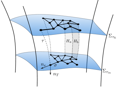
Figure 1: Shown is a portion of spacetime deconstructed in accordance with global hyperbolicity. Depicted is an (initial) hypersurface labeled by the time $\tau_{\mathrm{in}}$ assigned to the instantaneous events supported on $\Sigma_{\tau_{\mathrm{in}}}$ by freely falling observers. On this hypersurface an ideal network resides. As the network is freely falling to $\Sigma_{\tau_{\mathrm{fi}}}$ it traces out a piecewise smooth two-dimensional Lorentzian history to which the dynamical degrees of freedom are confined. As an example, in gray is shown the Lorentzian history traced out by the evolution of two edges of the network.

.

In these investigations the metric graph was considered as a fundamental structure. In our new approach, however, networks are implemented not only as a support for fields or differential operators, but a paramount importance is given to their Lorentzian histories. That means, quantum networks are embedded in a spacetime and are now employed as diagnostic devices to probe the embedding background by the sole means of the physics on the graph. In this perspective, ideal networks serve as playgrounds to capture physical properties of phenomena in spacetime. The advantages of this approach are set by the following remarks: 1. Embedding a network in a background induces a conformally flat metric on each of its edges. This implies that equation of motions are exact solvable, an extremely handy property when studying phenomena in curved and dynamical spacetimes, for which often a full $(1+3)$-dimensional approach and solution is not accessible. 2. Being confined on the network, the field theory is two-dimensional on each edge history. Hence, the field theory on the network reduces to a sum of simple $(1+1)$-dimensional theories supplied by appropriate boundary conditions at each vertex. Whenever a phenomenon or theory is well known in $(1+1)$-dimensions, its generalisation to the whole network follows systematically. An overview on different possible applications, ranging from curved spacetime frameworks, e.g. black hole physics to gravitational wave detection is presented for the reader in the outlook section.

In this work we employ ideal networks as diagnostic devices to evaluate entanglement properties of quantum fluctuations confined to network histories. For convenience we choose the entropy of entanglement as a measure for the entanglement of vacuum fluctuations. It is well-known that this measure requires a local finite resolution structure in order to avoid a short-distance completion including a fundamental description of gravity Witten (2018); Bombelli et al. (1986). Choosing a finite resolution structure amounts to introducing a short-distance scale corresponding to a minimal separation of the entangling quantum fluctuations. In experiments such a scale may be given by the finite width of the border across which the entanglement is probed or any other spatial resolution limit of the hardware infrastructure. Any separation scale provided by a characterisation of the extrinsic infrastructure has to be taken into account simply because it grants predictive power, and it is not flowing with the renormalisation group that takes care of the multi-scale phenomena created by the dynamical degrees of freedom.

It is essential to distinguish networks from (numerical) lattices even when the former are equipped with a regulatory structure. In this work graphs are introduced as a physical infrastructure and not as a discretisation scheme. Furthermore, any physical statement concerning quantum information measures or other observables is solely based on studying degrees of freedom supported by these infrastructures or their Lorentzian histories as two-dimensional submanifolds with boundaries embedded in spacetime. In particular, we show how quantum information properties of fields in spacetime can be captured by confining these fields on adapted networks and studying their entanglement properties in a strictly two-dimensional arena. In this sense the entanglement properties of fluctuations experiencing the full spacetime are an emergent phenomenon of those fields confined to the lower dimensional network histories. Alternatively, certain networks can conveniently be employed to capture quantum information properties that are supported in their embedding geometry.

Since graphs are idealised networks they can be used to describe physical aspects of systems on two-dimensional Lorentzian histories provided the idealisations are not interfering with the measurement accuracy envisaged in dedicated experiments. A formidable example for this is the recent experimental verification Tajik et al. (2023) of the area law of mutual information by employing effectively two-dimensional ultra-cold atom simulators to probe entanglement properties predicted in quantum field theory Bombelli et al. (1986) Srednicki (1993). At zero temperature and for pure states, the mutual information is equal to twice the entanglement entropy of either of the subsystems. In this experiment the finite resolution structure is determined by the resolution of the imaging system which limits access to shorter wavelength modes and enforces a short-distance cut-off. A comparison with the data of this experiment is shown in Figure 2.

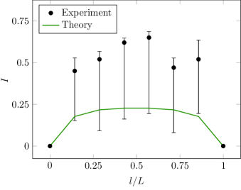
Figure 2: Shown are the mutual information $I$ of quantum fluctuations confined to a single edge in a low-temperature thermal state (data points) and in the ground state at zero temperature (our prediction) as a function of the subsystem size $l$ in fractions of the edge length $L$.

It should be noted that the experiment employed a Bose gas at temperatures between ten and 100 nano-Kelvin. So the quantum fluctuations that are accessible in accordance with the regulatory structure are in a thermal state resulting in an overpopulation relative to the ground state which we assume in our work.

This article is organized as follows: In Sec. II we provide a mathematical description of graphs and their histories as idealisation of physical networks. Together with the embedding of the network in an arbitrary spacetime, we derive the action and the equations of motion for a scalar field theory on the graph. In Sec. III, we move to quantum networks, i.e. we analyse quantum properties of a quantum scalar field confined on graphs. As a first investigation, we study the entanglement entropy of vacuum fluctuations confined on minimal graph configurations embedded in Minkowski. Sec. IV is finally devoted to the investigation of entanglement entropy of vacuum fluctuations confined on more general networks. The area scaling of the entanglement entropy and its dependence on the shape of the traced out region is investigated. Related discussions and further exciting applications of network histories are finally presented in Sec. V. Throughout this article, we use the metric signature diag$(-,+,+,+)$ and units where $c=G=\hbar=1$.

II Network histories

In this work, networks or graphs are meant as collections of objects, called nodes or vertices, and edges which connect them. More precisely, networks are ordered triples $\mathcal{N}=(N,E,\iota)$, assumed to be irreducible, consisting of a finite set $N$ of nodes, a finite set $E$ of edges, and an incident function $\iota:E\rightarrow N\times N$ mapping every edge to an unordered pair of not necessarily distinct nodes. Circumstances permitting, physical networks can be modelled as irreducible multi-graphs, where the connections are idealised as edges. For simplicity, physical networks and their idealisations will be denoted by the same triple. Throughout this discussion, we explore various perspectives on network configurations. We consider networks with either deformable or rigid edges, those that are in free fall or stationary at a particular location, and networks composed of physical matter or conceptualized as theoretical constructs. Specifically, in this section, we focus on a freely falling network with deformable edges, composed of physical matter, as illustrated in Fig. 1.

Let $(M,g)$ be a globally hyperbolic spacetime. The finite history of each edge $e$ in $(M,g)$ is a two-dimensional compact and connected Lorentzian submanifold $(H,h)$ of $(M,g)$, where $h$ is the pullback of the spacetime metric $g$ to $H$. Let $U$ be an open subset of the parameter plane $\mathbb{R}^{2}$ such that horizontal and vertical lines intersect $U$ either in intervals or not at all. The history or worldsheet of each edge $e$ in $E$ is given by a smooth two-parameter map $P:U\rightarrow H$, $(\tau,\sigma)\mapsto P(\tau,\sigma)$, which is composed of two families of one-parameter curves: The $\tau$-parameter curve $\sigma=\sigma_{0}$ of $P$ is $\tau\rightarrow P(\tau,\sigma_{0})$, and the $\sigma$-parameter curve $\tau=\tau_{0}$ of $P$ is $\sigma\rightarrow P(\tau_{0},\sigma)$.

We can think of the embedding of an edge on $H\subset M$ as a representation of this edge on $H$, where its nodes correspond to points of $H$ and the edge is a homeomorphic image of the $\sigma$- parameter curve such that the endpoints of this image coincide with the nodes of the edge.

In this work, networks represent spatial support structures for physical degrees of freedom in the following sense: The spacetime domains of observables are assumed to be confined to network histories embedded in spacetime.

This requires some geometrical preliminaries. Smooth $M$ vector fields $V$ on $H$ assign to each point of $H$ a tangent vector to $M$ at this point such that $V(f)$ is a smooth real-valued function on $H$, provided $f$ is a smooth real-valued function on $M$. The set of all such vector fields is denoted by $\overline{\mathrm{Vec}}(H)$ and is a module over the set of smooth real-valued functions on $H$. The unique Levi-Civita connection $D$ of $(M,g)$ induces a connection on $H\subset M$ in a natural way. Locally, smooth local extensions of $V\in\overline{\mathrm{Vec}}(H)$ and $X\in\mathrm{Vec}(H)$ can be constructed, and $D_{X}V$ can be defined using the extended vector fields and then restricting the Levi-Civita connection accordingly. Since the induced connection $D:\mathrm{Vec}(H)\times\overline{\mathrm{Vec}}(H)\rightarrow\overline{\mathrm{Vec}}(H)$ defined above is closely related to the Levi-Civita connection on $M$, we use the same symbol for both.

II.1 Classical fields populating network histories

In this section we discuss the covariant theory of classical fields confined to a given network infrastructure embedded in a globally hyperbolic spacetime. The network metric required for the kinetic operator of these classical fields corresponds to the spacetime geometry induced on the network. Hence, the spacetime metric is the only classical field that is not confined to the network.

II.2 Action and data storage

Let $\mathcal{N}=(N,E,\iota)$ be a network that is piecewise embedded in a globally hyperbolic spacetime $(M,g)$, that is each edge in $E$ is embedded in $(M,g)$ (subject to boundary conditions). Let $n:=\sharp E$ denote the cardinality of $E$. We equip each edge history $H_{a}$, $a\in\{1,\cdots,n\}\subset\mathbb{N}$ with a configuration bundle $\mathcal{C}_{a}$ and, for simplicity, choose real vector bundles of rank one: $\mathcal{C}_{a}:=(C_{a},\pi_{a},H_{a},\mathbb{R})$. Configuration fields on $H_{a}$ are sections of $\mathcal{C}_{a}$, collectively collected in the space $\Gamma_{\mathrm{c}}(H_{a},C_{a})\subset\Gamma(H_{a},C_{a})$ of compactly supported smooth sections on $H_{a}$. Sections of the dual bundle $\pi_{a}^{*}:C_{a}^{*}\rightarrow H_{a}$, or, equivalently $\mathrm{Hom}(C_{a},\mathbb{R}\times H_{a})$, serve as dual configuration fields. In particular, $\Gamma_{c}(H_{a},C_{a}^{*})$ contains linear evaluation forms, which are convenient to represent the classical field theory in a language close to the one used for the corresponding quantum theory.

Locality is made manifest by a Lagrangian of order $k$, $L_{a}:J^{k}\mathcal{C}_{a}^{*}\rightarrow\Omega_{2}(H_{a})$, which is a bundle morphism between the $k$-th jet bundle of $\mathcal{C}_{a}^{*}$, called the Lagrangian phase bundle, and the bundle of two-forms over $H_{a}$. The action functional $\mathcal{A}_{a}(\varphi):\Gamma(H_{a},C_{a})\rightarrow\mathbb{R}$ is given by

$$\mathcal{A}_{a}(\varphi):=\int_{H_{a}}\;s\cdot(L_{a}\circ j^{k}\varphi)+\mathcal{B}_{a}(\varphi)\;,$$ (1)

where $\varphi\in\Gamma(H_{a},C_{a}^{*})$, $s$ is a compactly supported test section in $\Gamma_{\mathrm{c}}(H_{a},C_{a})$, and $\mathcal{B}_{a}(\varphi)$ denotes a functional that specifies conditions along the boundary $\partial H_{a}$ of $H_{a}$. Relative to an abstract coordinate system $(x,\varphi)$ in the configuration bundle $\mathcal{C}_{a}^{*}$, a Lagrangian of order one is represented by $\mathcal{L}_{a}(x,\varphi,\mathrm{d}\varphi)\;\mathrm{dvol}_{h_{a}}$ on the associated coordinate neighbourhood, where $\mathrm{dvol}_{h_{a}}$ denotes the natural volume element in $(H_{a},h_{a})$, and the local map $\mathcal{L}_{a}$ is the usual Lagrange density.

Consider a vertical vector field $X$ over $\mathcal{C}_{a}^{*}$ that is required to vanish over the boundary $\partial H_{a}$, and denote its flow by $F_{t}:\mathcal{C}^{*}\rightarrow\mathcal{C}^{*}$, which is a one-parameter subgroup of vertical automorphisms of the dual configuration bundle. This allows to define a one-parameter family of sections by $\varphi_{t}:=F_{t}\circ\varphi$ and consider their actions $\mathcal{A}_{a}(\varphi_{t})$. The variation of the action along the deformation over $H$ of the action at $\varphi$ is $(\delta_{X}\mathcal{A}_{a})(\varphi)=\tfrac{\mathrm{d}}{\mathrm{d}t}\mathcal{A}_{a}(\varphi_{t})|_{t=0}$. Classical solutions are sections of the bundle $\mathcal{C}_{a}^{*}$ at which the action is stationary.

The network data is stored as follows: Consider a network $\mathcal{N}=(N,E,\iota)$ and let $H_{\mathcal{N}}=\cup_{a=1}^{n}H_{a}$ be its connected, piecewise smooth history relative to a global hyperbolic spacetime $(M,g)$. Introduce the network action functional $\mathcal{A}_{H}$ $:$ $\oplus_{a=1}^{n}\Gamma(H_{a},C_{a}^{*})$ $\rightarrow$ $\oplus_{a=1}^{n}\Gamma(H_{a},C_{a}^{*})$, defined by $\mathcal{A}_{H}(\varphi^{1},\cdots,\varphi^{n}):=(\mathcal{A}_{1}(\varphi^{1}),\cdots,\mathcal{A}_{n}(\varphi^{n}))$. For any $F$ in $\oplus_{a=1}^{n}\Gamma(H_{a},C_{a}^{*})$, let us write $F=(F^{1},\cdots,F^{n})$ with $F^{a}\in\Gamma(H_{a},C_{a}^{*})$ and identify $F^{a}$ with $(0^{1},\cdots,F^{a},\cdots,0^{n})$, where $0^{a}$ denotes the zero section in $\Gamma(H_{a},C_{a}^{*})$. In this notation, assuming $A_{a}(\varphi^{a})$ is a functional of degree equal to or larger than one, $\mathcal{A}_{H}(\varphi)$ is identified with $(\mathcal{A}_{H}(\varphi^{1}),\cdots,\mathcal{A}_{H}(\varphi^{n}))$ since $\mathcal{A}_{H}(\varphi^{a})=(0^{1},\cdots,\mathcal{A}_{a}(\varphi^{a}),\cdots,0^{n})$.

In order to appreciate networks in the given context, we discuss the dynamics of fields populating completely disjoint edges and compare it to the dynamics on basic building blocks of faithful networks. For this, the following concept proves useful: Let $\langle\cdot,\cdot\rangle_{a}$ denote the pairing $\Gamma_{\mathrm{c}}(H_{a},C_{a})\times\Gamma(H_{a},C_{a}^{*})$ $\rightarrow$ $\Gamma_{\mathrm{c}}(H_{a},C_{a}^{*})$, where $\langle f,F\rangle_{a}$ is defined to be the integral of $f_{a}F^{a}$ over the compact support of $f_{a}$, $\text{supp}(f_{a})\subset H_{a}$ with respect to the canonical measure given by the metric $h_{a}$.

II.3 Decoupled theory

Consider a system of $n$ disconnected freely falling edges, populated by classical fields. We refer to this as a decoupled theory with action $\sum_{a=1}^{n}\mathcal{A}_{H}(\varphi^{a})$ with $\mathcal{A}_{H}(\varphi^{a})=\mathcal{A}_{H}^{\;\mathrm{free}}(\varphi^{a})$ $+$ $\mathcal{B}_{H}(\varphi^{a})$, where $\mathcal{A}_{H}^{\;\mathrm{free}}(\varphi^{a})$ is given by a quadratic Lagrangian of order one, describing the free evolution on the edge $e_{a}$, $a\in\{1,\cdots,n\}$, and $\mathcal{B}_{H}(\varphi^{a})$ is given by a linear Lagrangian of order zero, describing Dirichlet boundary conditions on $\partial H_{a}$ via Lagrange multiplier fields $\lambda_{d}$, $d\in\{1,\cdots,4\}$.

The boundary $\partial H_{a}$ of a finite history $H_{a}$ can be described as follows: Let $U$ be an open subset of the parameter plane $\mathbb{R}^{2}$ and $\tau_{\mathrm{in}},\tau_{\mathrm{fi}},\sigma_{\mathrm{f}}^{1},\sigma_{\mathrm{f}}^{2}$ be history parameters in $U$ such that $\partial_{\mathrm{f}}^{1}e_{a}:[\tau_{\mathrm{in}},\tau_{\mathrm{fi}}]$ $\rightarrow H_{a}$, $\tau\mapsto\partial_{\mathrm{f}}^{1}e_{a}(\tau):=P_{a}(\tau,\sigma_{\mathrm{f}}^{1})$, is the worldline of a free endpoint of edge $e_{a}$ in the history $H_{a}$, and accordingly for the other free endpoint $\partial_{\mathrm{f}}^{2}e_{a}$ of $e_{a}$. Furthermore, $\partial_{\mathrm{in}}T_{a}:[\sigma_{\mathrm{f}}^{1},\sigma_{\mathrm{f}}^{2}]$ $\rightarrow H_{a}$, $\sigma\mapsto\partial_{\mathrm{in}}T_{a}(\sigma)$ $:=P_{a}(\tau_{\mathrm{in}},\sigma)$ describes the edge $e_{a}$ at initial parameter time in $H_{a}$, and, accordingly, $\partial_{\mathrm{fi}}T_{a}$ gives the same edge at final parameter time $\tau_{\mathrm{fi}}$ in $H_{a}$. Now we introduce projections onto the above boundary segments: For $i\in[2]$, $p\in H_{a}$, $\mathcal{X}_{\partial_{\mathrm{f}}^{i}e_{a}}(p)\cdot\varphi^{a}(p)(\phi_{a})$ $:=\phi_{a}(p)$ if $p$ lies on the worldline of the specified free endpoint of $e_{a}$ in $H_{a}$, and zero otherwise. Furthermore, for $A\in\{\mathrm{in},\mathrm{fi}\}$, $q\in H_{a}$, $\mathcal{X}_{\partial_{\mathrm{A}}T_{a}}(q)\cdot\varphi^{a}(q)(\phi_{a})$ $:=\phi_{a}(q)$ if $q$ is located on $e_{a}$ at the specified time, and zero otherwise.

Consider $\mathcal{A}_{H}^{\;\mathrm{free}}(\varphi^{a})$ $=$ $\langle s,-\tfrac{1}{2}h^{-1}(\mathrm{d}\varphi,\mathrm{d}\varphi)\rangle_{a}$ with a compact smearing section $s\in\Gamma_{\mathrm{c}}(H_{a},C_{a})$, where we used the pairing introduced above. And, $\mathcal{B}_{H}(\varphi^{a})=\langle s,\mathcal{X}_{\partial_{\mathrm{f}}^{1}e}\,\lambda_{1}\varphi\rangle_{a}$ $+$ $\langle s,\mathcal{X}_{\partial_{\mathrm{f}}^{2}e}\,\lambda_{2}\varphi\rangle_{a}$ $+$ $\langle s,\mathcal{X}_{\partial_{\mathrm{in}}T}\,\lambda_{3}\varphi\rangle_{a}$ $+$ $\langle s,\mathcal{X}_{\partial_{\mathrm{fi}}T}\,\lambda_{4}\varphi\rangle_{a}$. These boundary terms enforce Dirichlet boundary conditions for classical fields populating $n$ freely falling edges, i.e. $\phi_{a}=0$ on the $2n$ worldlines of the free endpoints, and $\phi_{a}=0$ for the $2n$ field configurations on the edge at the initial and final time.

The dynamical content requires little more work: As above, consider a vertical vector field $X_{a}$ over $C_{a}^{*}$. Setting $f_{a}:=X_{a}(\varphi^{a})$ and choosing the support functions $s_{a}$ in $\mathcal{A}_{H}^{\mathrm{free}}(\varphi^{a})$ such that $s_{a}=1$ on the support of $f_{a}$, we have $(X_{a}\mathcal{A}_{H}^{\mathrm{free}}(\varphi^{a}))(\phi_{a})=\langle f,\Box_{h}\phi\rangle_{a}+\mathcal{S}_{H}(\varphi^{a})(\phi_{a})$. The surface term is given by

$$\mathcal{S}_{H}(\varphi^{a})(\phi_{a}) = \left\langle f,\left[\mathcal{X}_{\partial_{A}T}\right]_{\mathrm{in}}^{\mathrm{fi}}D_{n_{T}}\phi+[\mathcal{X}_{\partial_{\mathrm{f}}^{i}e}]_{\mathrm{1}}^{\mathrm{2}}\,D_{n_{e}}\phi\right\rangle_{a}\;.$$

Here, $n_{T}\perp\partial_{\mathrm{in}}T$ is chosen to be a past-pointing vector field normal to the initial edge in $H_{a}$, and $n_{e}$ is a vector field normal to the worldline of $\partial_{\mathrm{f}}^{1}e$ in $H_{a}$, oriented away from the edge. Furthermore, $[\zeta_{\nu}]^{\alpha}_{\beta}:=\zeta_{\alpha}-\zeta_{\beta}$. A straightforward calculation gives for the variation of the boundary action $(X_{a}\mathcal{B}_{H}(\varphi^{a}))(\phi_{a})$ $=$ $\langle f,\mathcal{X}_{\partial_{\mathrm{f}}^{1}e}\lambda_{1}\rangle_{a}$ $+$ $\langle f,\mathcal{X}_{\partial_{\mathrm{f}}^{2}e}\lambda_{2}\rangle_{a}$ $+$ $\langle f,\mathcal{X}_{\partial_{\mathrm{in}}T}\lambda_{3}\rangle_{a}$ $+$ $\langle f,\mathcal{X}_{\partial_{\mathrm{fi}}T}\lambda_{4}\rangle_{a}$.

The wave equation for classical fields on a system of freely falling, disjoint edges with Dirichlet conditions imposed on the boundaries of the respective histories is given by

$$\Box_{h}\phi+\big{[}\mathcal{X}_{\partial_{A}T}\,D_{n_{T}}\phi\big{]}_{\mathrm{in}}^{\mathrm{fi}}+\big{[}\mathcal{X}_{\partial_{f}^{i}e}D_{n_{e}}\phi\big{]}_{\mathrm{1}}^{\mathrm{2}}$$

$$=-\mathcal{X}_{\partial_{\mathrm{f}}^{1}e}\lambda_{1}-\mathcal{X}_{\partial_{\mathrm{f}}^{2}e}\lambda_{2}-\mathcal{X}_{\partial_{\mathrm{in}}T}\lambda_{3}-\mathcal{X}_{\partial_{\mathrm{fi}}T}\lambda_{4}\;,$$ (2)

where we suppressed the edge label for ease of notation. On the interior of each history $H_{a}$, we find $\Box_{h}\phi=0$. Using this in (II.3), we can solve for the Lagrange multiplier fields:

$$\lambda_{1} = -\Box_{h}\phi\;\big{|}_{\partial_{\mathrm{f}}^{1}e}-D_{n_{e}}\phi-\big{[}\mathcal{X}_{\partial_{A}T}\,D_{n_{T}}\phi\big{]}_{\mathrm{in}}^{\mathrm{fi}}\;\big{|}_{\partial_{\mathrm{f}}^{1}e}\;,$$

$$\lambda_{2} = -\Box_{h}\phi\;\big{|}_{\partial_{\mathrm{f}}^{2}e}+D_{n_{e}}\phi-\big{[}\mathcal{X}_{\partial_{A}T}\,D_{n_{T}}\phi\big{]}_{\mathrm{in}}^{\mathrm{fi}}\;\big{|}_{\partial_{\mathrm{f}}^{2}e}\;,$$

$$\lambda_{3} = -\Box_{h}\phi\;\big{|}_{\partial_{\mathrm{in}}T}+D_{n_{T}}\phi-\big{[}\mathcal{X}_{\partial_{\mathrm{f}}^{i}e}\,D_{n_{T}}\phi\big{]}_{1}^{2}\;\big{|}_{\partial_{\mathrm{in}}T}\;,$$

$$\lambda_{4} = -\Box_{h}\phi\;\big{|}_{\partial_{\mathrm{fi}}T}-D_{n_{T}}\phi-\big{[}\mathcal{X}_{\partial_{\mathrm{f}}^{i}e}\,D_{n_{T}}\phi\big{]}_{1}^{2}\;\big{|}_{\partial_{\mathrm{fi}}T}\;.$$ (3)

Notice that at the free endpoints, we can rewrite the first two equations as:

$$D_{n_{e}}\phi\big{|}_{\partial_{\mathrm{f}}^{1}e}\ = -\lambda_{1}+\big{[}\mathcal{X}_{\partial_{A}T}\,D_{n_{T}}\phi\big{]}_{\mathrm{in}}^{\mathrm{fi}}\;\big{|}_{\partial_{\mathrm{f}}^{1}e}\;,$$

$$D_{n_{e}}\phi\big{|}_{\partial_{\mathrm{f}}^{2}e}\ = \lambda_{2}+\big{[}\mathcal{X}_{\partial_{A}T}\,D_{n_{T}}\phi\big{]}_{\mathrm{in}}^{\mathrm{fi}}\;\big{|}_{\partial_{\mathrm{f}}^{2}e}$$ (4)

where the right hand sides are constants. The above equations guarantee a constant field derivative at the boundaries, thereby enforcing total reflection and consequently preventing any flux leakage from the network.

II.4 Coupled theory

Next, we allow connections of edges into nodes. The minimal network we can consider is a freely falling star graph, that is a network consisting of $n$ edges each connected to all others at a single vertex, and each populated by classical fields with action $\mathcal{A}_{H}(\varphi^{a})$ $=$ $\mathcal{A}_{H}^{\mathrm{free}}(\varphi^{a})$ $+$ $\mathcal{B}_{H}(\varphi^{a})$ $+$ $\mathcal{C}_{H}(\varphi^{a})$. A star graph serves as the fundamental building block for more complex networks, hence by introducing the theory for such a minimal junction, we inherently provide a theoretical framework applicable to networks of arbitrary configurations.

Without loss of generality, let the joining vertex $\partial_{\mathrm{j}}e_{a}$ be indexed with label j. The boundary action $\mathcal{B}_{H}(\varphi^{a})$ needs to be adapted to this setting, which amounts to Dirichlet conditions for the $n$ free endpoints. For finite histories $H_{a}$, the temporal boundary conditions remain the same as in the decoupled theory. So instead of having $4n$ Dirichlet conditions, the boundary action now specifies only $3n$ conditions for the star graph setting. The remaining $n$ conditions are provided by the coupling action, whereby one is trivial: Introduce the two-edge coupling functional by $\mathcal{C}_{an}$ $=$ $[\langle s,\lambda^{\mathrm{c}}\mathcal{X}_{\partial_{\mathrm{j}}e}\varphi\rangle_{i}]^{a}_{n}$. The star-graph coupling action is just a sum over all edges of these two-edge coupling forms, yielding the following coupling conditions at the joining node for each adjacent edge $a$: $\mathcal{X}_{\partial_{\mathrm{j}}e_{a}}\phi_{a}$ $=$ $\mathcal{X}_{\partial_{\mathrm{j}}e_{n}}\phi_{n}$, that is, the field configurations are continuous across the worldline of the joining vertex. This specific choice of coupling conditions accounts for the so called Kirchhoff-Neumann conditions (which reduce to the known Neumann conditions for $n=2$). By imposing continuity of the field configurations, Kirchhoff-Neumann conditions ensure energy conservation at each vertex, which will act neither as a sink nor as a source for the field. In general, different choice of coupling conditions will lead to describing different physical setups. Since in this article we aim to describe physical networks as webs of communication channels, we demand each vertex of the idealized graph to be physically analogous to a node in electrical currents -for which what enters in has to come out- condition ensured by the Kirchhoff-Neumann conditions.

The wave equation for classical fields populating a star network with Dirichlet boundary and coupling conditions imposed is given by

$$\Box_{h_{a}}\phi_{a}+\big{[}\mathcal{X}_{\partial_{A}T_{a}}D_{n_{T_{a}}}\phi_{a}\big{]}^{\mathrm{fi}}_{\mathrm{in}}+\big{[}\mathcal{X}_{\partial_{\mathrm{r}}e_{a}}D_{n_{e_{a}}}\phi_{a}\big{]}^{\mathrm{f}}_{\mathrm{j}}=$$

$$=-\mathcal{X}_{\partial_{\mathrm{f}}e_{a}}\lambda_{1a}-\mathcal{X}_{\partial_{\mathrm{in}}T_{a}}\lambda_{2a}-\mathcal{X}_{\partial_{\mathrm{fi}}T_{a}}\lambda_{3a}+$$

$$\;\;\;\;-\left(1-\delta_{an}\right)\mathcal{X}_{\partial_{\mathrm{j}}e_{a}}\lambda_{a}^{\mathrm{c}}+\delta_{an}\mathcal{X}_{\partial_{\mathrm{j}}e_{n}}\sum_{b\in[n-1]}\lambda_{b}^{\mathrm{c}}\;,$$ (5)

On the interior of $H_{a}$, Eq. (II.4) reduces to $\Box_{h_{a}}\phi_{a}=0$. Using this in (II.4), we determine the Lagrange multiplier fields associated with the Dirichlet boundary segments at the extremities of the star graph:

$$\lambda_{1a} = -\Box_{h_{a}}\phi_{a}\big{|}_{\partial_{\mathrm{f}}e_{a}}-D_{n_{e_{a}}}\phi_{a}-\big{[}\mathcal{X}_{\partial_{A}T_{a}}D_{n_{T_{a}}}\phi_{a}\big{]}^{\mathrm{fi}}_{\mathrm{in}}\big{|}_{\partial_{\mathrm{f}}e_{a}}\;,$$

$$\lambda_{2a} = -\Box_{h_{a}}\phi_{a}\big{|}_{\partial_{\mathrm{in}}T_{a}}+D_{n_{T_{a}}}\phi_{a}-\big{[}\mathcal{X}_{\partial_{r}e_{a}}D_{n_{e_{a}}}\phi_{a}\big{]}^{\mathrm{f}}_{\mathrm{j}}\big{|}_{\partial_{\mathrm{in}}T_{a}}\;,$$

$$\lambda_{3a} = -\Box_{h_{a}}\phi_{a}\big{|}_{\partial_{\mathrm{fi}}T_{a}}-D_{n_{T_{a}}}\phi_{a}-\big{[}\mathcal{X}_{\partial_{r}e_{a}}D_{n_{e_{a}}}\phi_{a}\big{]}^{\mathrm{f}}_{\mathrm{j}}\big{|}_{\partial_{\mathrm{fi}}T_{a}}\;.$$

In addition, for the internal vertex we find the Lagrange multiplier fields associated with the coupling of the edges to a star network:

$$\lambda_{a}^{\mathrm{c}}=-\Box_{h_{a}}\phi_{a}\big{|}_{\partial_{\mathrm{j}}e_{a}}+D_{n_{e_{a}}}\phi_{a}-\big{[}\mathcal{X}_{\partial_{A}T_{a}}D_{n_{T_{a}}}\phi_{a}\big{]}^{\mathrm{fi}}_{\mathrm{in}}\big{|}_{\partial_{\mathrm{j}}e_{a}}\;,$$

$$\sum_{b\in[n-1]}\lambda_{b}^{\mathrm{c}}=$$

$$=-\Box_{h_{n}}\phi_{n}\big{|}_{\partial_{\mathrm{j}}e_{n}}-D_{n_{e_{n}}}\phi_{n}-\big{[}\mathcal{X}_{\partial_{A}T_{n}}D_{n_{T_{n}}}\phi_{n}\big{]}^{\mathrm{fi}}_{\mathrm{in}}\big{|}_{\partial_{\mathrm{j}}e_{n}}\;,$$ (7)

for $a\in\{1,\cdots,n-1\}$. Given the network’s orientation, the second equation in (II.4) is a typical example for a collection of conservation laws associated with the internal vertex. For instance, power counting arguments allow to extract from (II.4) the following statements:

$$\Box_{h_{n}}\phi_{n}\big{|}_{\partial_{\mathrm{j}}e_{n}} = \sum_{a\in[n-1]}\Box_{h_{a}}\phi_{a}\big{|}_{\partial_{\mathrm{j}}e_{a}}\;,$$

$$D_{e_{n}}\phi_{n}\big{|}_{\partial_{\mathrm{j}}e_{n}} = -\sum_{a\in[n-1]}D_{n_{e_{a}}}\phi_{a}\big{|}_{\partial_{\mathrm{j}}e_{a}}\;.$$ (8)

The last equation can be rewritten as:

$$\sum_{a\in[n]}D_{n_{e_{a}}}\phi_{a}\big{|}_{\partial_{\mathrm{j}}e_{a}}=0\;.$$ (9)

Together with the smoothness condition for the field across the worldline of the node, this equation ensures that fluxes can propagate across the vertex and that the node does not act as a source or a sink, thereby ensuring energy conservation. As already mentioned, these junction conditions are commonly referred to as the Kirchhoff-Neumann conditions.

III Entanglement on network histories

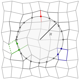
Figure 3: Spatial section of a three-dimensional mesh graph embedded in Minkowski spacetime. The disk of radius $R$ is traced out and the crossing points of this circle and the graph are indicated with dots. The single edge shown in red, the simple loop in blue, and star graph with three edges depicted in green represent basic building blocks of this graph. Moreover, a sub-graph consisting of this star graph and two additional edges (dashed) is shown as an example for a loop with a single edge attached.

An example of a general network can be thought of as the mesh graph depicted in Fig. 3. Evolving edges trace out two-dimensional Lorentzian histories to which we assign actions (1) including boundary specifications like the Kirchhoff-Neumann boundary conditions, as explained in section 9.

While we discussed above rudiments of (classical) field theory on network histories in a covariant framework, entanglement measures require a canonical treatment. Locality is made manifest by Hamiltonian densities $\mathcal{H}=\tfrac{1}{2}\pi^{2}+V_{\mathrm{eff}}(\phi)$ on momentum phase-spaces $T^{*}\mathcal{C}_{e}$ consisting of points $(\pi,\phi)$, with $\pi$ denoting the momentum conjugated to the configuration field $\phi$ in each fiber over the edge $e$ under consideration. The finite resolution structure can be introduced by mimicking smearing prescriptions as follows: Let us assume there is a short-distance regulator $a$ given by the experiment in question. Set $\mathrm{grad}\,\phi=a^{-1}(T_{a}-\mathrm{id}_{\mathcal{C}_{e}})\phi$, where $T_{a}$ denotes a spatial translation by $a$. The above equality is exact in the sense of Newtonian calculus for infinitesimal quantities and its deviation from the limit are well below the experimental resolution limit. Furthermore, let $\mathcal{R}$ be a locally finite collection of countably many points in the interior of the edge and denote by $\mathcal{X}_{\mathcal{R}}(\cdot)$ its indicator function. The Hamiltonian adapted to this specific finite resolution structure is simply given by

$$H_{\mathcal{R}}:=\int_{e}\mathcal{X}_{\mathcal{R}}\cdot\mathcal{H}\;,$$ (10)

which needs to be supplemented by appropriate boundary conditions.

In the remainder of this article we demonstrate the usefulness of quantum networks for entanglement diagnostics. For simplicity we consider adapted networks in Minkowski spacetime and use them to evaluate entanglement properties of free quantum fluctuations in the Poincaré invariant vacuum.

In this chapter, we consider the general network depicted in Fig. 3, but focusing at first on its three basic building blocks: A single edge, a loop and the special case of a star graph consisting of three edges joined together at a single vertex.

III.1 Entanglement diagnostics in $\mathbb{R}_{1,1}$

We choose a finite resolution structure characterised by the set $\{a,\cdots,Na\}$, with $a=const.\in\mathbb{R}$, $N\in\mathbb{N}$, on each edge of the network. $L=Na$ is the long-distance scale and length of the edge. Introducing the inner product $\langle F_{1},F_{2}\rangle_{e}$ of phase space functions $F_{1}$ and $F_{2}$ by integrating $\mathcal{X}_{\mathcal{R}}\cdot F_{1}\cdot F_{2}$ over the edge, the Hamiltonian for a free quantum field $\phi$ of mass $\mu$ confined to a single edge is given by (after appropriate re-scaling)

$$H_{\mathcal{R}}=\frac{1}{2a}\big{(}\left\langle\pi,\pi\right\rangle_{e}+\left\langle\phi,\mathcal{K}(\phi)\right\rangle_{e}\big{)}\;,$$ (11)

where $\mathcal{K}$ is a bi-local functional which is represented by the $(N\times N)$-matrix $K$ relative to the chosen finite resolution structure:

$$K=M^{2}E+\Delta_{\mathrm{l}}\left(K\right)+\Delta_{\mathrm{u}}(K).$$ (12)

Here, $E$ denotes the unit matrix, $M^{2}:=\tfrac{1}{N}\mathrm{tr}(K)=2+\mu^{2}a^{2}$, $\mathrm{tr}(K)$ is the trace of $K$, $\Delta_{\mathrm{l}}(K)$ and $\Delta_{\mathrm{u}}(K)$ are the lower and upper triangular submatrices of the matrix $K-M^{2}E$, respectively, given by $(\Delta_{\mathrm{l}}(K))_{qs}=-\theta(N-s-1/2)\delta_{q,s+1}$ and $(\Delta_{\mathrm{u}}(K))_{qs}=-\theta(N-q-1/2)\delta_{q+1,s}$.

At first, we want to study entanglement properties along one single edge of the network only. To this aim, we consider a single edge like the one shown in red in Fig. 3 and impose Dirichlet boundary conditions at its endpoints. In this way, we decouple it from the network and we can consider it independently.

In the case at hand, the lower triangular submatrix can be transformed into the upper one and vice versa by exchanging rows and columns. The indices give the multiples of $a$ along the edge, so $\phi_{q}:=\phi(qa)$. It is convenient to introduce $\bm{\phi}:=\phi_{s}\mathbf{e}_{s}$, where $(\mathbf{e}_{s})^{q}=\delta^{\;q}_{s}$, and $\mathbf{e}_{s}\cdot\mathbf{e}_{s}=\delta_{qs}$. In greater detail, relative to the finite resolution structure,

$$H_{\mathcal{R}}=\frac{1}{2a}\left(\bm{\pi}\cdot\bm{\pi}+\bm{\phi}\cdot\left(K\bm{\phi}\right)\right)\;.$$ (13)

We can find a unitary transformation $U$ from $\bm{\phi}$ to $\tilde{\bm{\phi}}$ which induces a similarity transformation on $\Omega:=\sqrt{K}$ that diagonalises it. The ground state $\Psi=\otimes_{q\in\lceil N\rfloor}\Psi_{q}$ of the system relative to the finite resolution structure is given by the wave function

$$\Psi(\bm{\phi})=\left(\mathrm{det}\left(\tfrac{\Omega}{\pi a^{2}}\right)\right)^{1/4}\exp{\left(-\tfrac{1}{2}\bm{\phi}\cdot\left(\Omega\bm{\phi}\right)\right)}\;.$$ (14)

In order to probe entanglement properties along the edge $e$, we split it into two parts $\mathrm{int}(e)$ and $\mathrm{ext}(e)$, which is concomitant with dividing the original system (mapped onto the finite resolution structure) into a subsystem referred to as interior (I) and a subsystem referred to as exterior (E). We decompose $\Omega$ accordingly Srednicki (1993); Bombelli et al. (1986):

$$\Omega=\begin{pmatrix}\Omega_{\mathrm{II}}&\Omega_{\mathrm{IE}}\\ \Omega_{\mathrm{EI}}&\Omega_{\mathrm{EE}}\end{pmatrix},$$ (15)

and similarly for $\Omega^{-1}$. We choose to compute the reduced density matrix $\rho_{\mathrm{E}}$ corresponding to the exterior subsystem, that is we integrate out the degrees of freedom localised in the interior subsystem, giving

$$\rho_{{\mathrm{E}}}\left(\bm{\phi},\bm{\phi^{\prime}}\right)\sim\exp{\left(-\tfrac{1}{2}\left(\bm{\phi}\cdot\left(\gamma\bm{\phi}\right)+\bm{\phi^{\prime}}\cdot\left(\gamma\bm{\phi^{\prime}}\right)\right)+\bm{\phi^{\prime}}\cdot\left(\beta\bm{\phi}\right)\right)}\;$$ (16)

where $\bm{\phi}$, $\bm{\phi^{\prime}}$ now refer to the exterior collection of configuration variables relative to the finite resolution structure. Furthermore, $\beta:=\tfrac{1}{2}\Omega_{\mathrm{IE}}\,{(\Omega_{\mathrm{II}})}^{-1}\,(\Omega_{\mathrm{IE}})^{\mathrm{T}}$, and $\gamma:=\Omega_{\mathrm{EE}}-\beta$.

In order to compute the eigenvalues of the reduced density matrix $\rho_{\mathrm{E}}$, we need to diagonalise it, which requires two more transformations: First, an orthogonal transformation $V$ of the configuration variables, $\bm{\phi}\mapsto\gamma^{1/2}_{\mathrm{diag}}(V\bm{\phi})$ so that $\gamma=:V^{\mathrm{T}}\gamma_{\mathrm{diag}}V$, where $\gamma_{\mathrm{diag}}$ is diagonal, and subsequently another orthogonal transformation $S$ of the new configuration variables that diagonalises $\Lambda:=\gamma_{\mathrm{diag}}^{-1/2}V\beta V^{\mathrm{T}}\gamma_{\mathrm{diag}}^{-1/2}$, so that $\Lambda=:S^{\mathrm{T}}\Lambda_{\mathrm{diag}}S$. For ease of notation we rename the transformed configuration variables by their old names. Then

$$\rho_{\mathrm{E}}\left(\bm{\phi},\bm{\phi^{\prime}}\right) \sim \prod_{\phi_{q},\phi^{\prime}_{q}\in\mathcal{C}_{\mathrm{ext}(e)}}\rho_{\mathrm{E}}\left(\phi_{q},\phi_{q}^{\prime}\right)\;,$$

$$\rho_{\mathrm{E}}\left(\phi_{q},\phi_{q}^{\prime}\right) = \exp{\left(-\tfrac{1}{2}\left(\phi_{q}^{2}+\phi_{q}^{\prime 2}\right)+\lambda_{q}\phi_{q}\phi_{q}^{\prime}\right)}\;,$$ (17)

where $\lambda_{q}$ is an eigenvalue of $\Lambda$. Given the eigenvalues of each $\rho_{\mathrm{E}}\left(\phi_{q},\phi_{q}^{\prime}\right)$ as $p_{n_{q}}=(1-\tilde{\xi}_{q})\tilde{\xi}_{q}^{n_{q}}$, with $n_{q}\in\mathbb{Z}$ and

$$\tilde{\xi}_{q}=\frac{\lambda_{q}}{1+\sqrt{1-\lambda_{q}^{2}}}\;,$$ (18)

we can write the spectrum of $\rho_{\mathrm{E}}\left(\bm{\phi},\bm{\phi^{\prime}}\right)$ as

$$p_{n_{n+1},\dots,n_{N}}=\prod_{s\in D}\left(1-\tilde{\xi}_{s}\right)\tilde{\xi}_{s}^{n_{s}}$$ (19)

where we defined $D:=\{q\in\lceil N\rfloor:qa\in\mathrm{ext}(e):=\left[(n+1)a,\dots,Na\right],n\in\mathbb{N}\}$. In this language, the total entropy $S$ of entanglement for massive quantum fluctuations in the ground state confined to a single edge is given by

$$S\left(\bm{\tilde{\xi}}\right) = \sum\limits_{s\in D}S_{s}\left(\tilde{\xi}_{s}\right)\;,$$

$$S_{s}\left(\tilde{\xi}_{s}\right) = -\mathrm{ln}\left(1-\tilde{\xi}_{s}\right)-\frac{\tilde{\xi}_{s}}{1-\tilde{\xi}_{s}}\;\mathrm{ln}\left(\tilde{\xi}_{s}\right)\;,$$ (20)

where again $D:=\{q\in\lceil N\rfloor:qa\in\mathrm{ext}(e)\}$.

For now we are only interested in the dependence of the entanglement entropy (III.1) on the set $D$, or referring to Fig. 3, we are interested in its dependence on the radius $R$ of the entangling sphere. In fact, as shown in Fig. 3, the entangling sphere radius defines the splitting of the red edge in two intervals: int(e) residing inside the entangling sphere, and ext(e) residing in its exterior. Hence, by tracing out a sphere of radius $R$ we in fact define the traced out interval int(e) on the edge with respect to which (III.1) is computed.

It is convenient to normalise the entanglement entropy relative to its value for (1.) a radius $R$ for which int(e) equals half the long-distance scale $L$ and for (2.) quantum fluctuations with masses $\mu$ so that $\mu a=10^{-1}$ for a short-distance scale $a$ provided by the experimental set-up: $\bar{S}(R)={S(R)}/{S(L/2)}$, where $R$ is measured in multiples of $L$.

We developed a code Giavoni et al. (2023) for computing the entanglement entropy of quantum fluctuations on networks that are intersected by entangling surfaces. For the single red edge shown in Fig. 3, the results of a numerical computation of $\bar{S}$ are presented in Fig. 4.

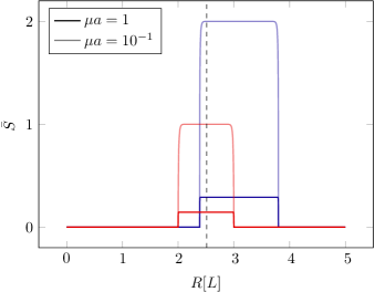
Figure 4: Entanglement entropy of quantum fluctuations confined to the basic building blocks of the mesh graph shown in Fig. 3 in terms of the radius of an entangling sphere. In particular, the entanglement entropy is given for the red edge and the blue loop equipped with a finite resolution structure consisting of $N=300$ locations for two different choices of $\mu a$. The radius of the entangling sphere shown in Fig. 3 is indicated with a vertical dashed line.

Referring to Fig. 3, the single edge intersects the entangling sphere once. For radii $R<2L$, the edge would not intersect the entangling sphere and the entanglement entropy for quantum fluctuations localised on the edge would be zero. Similarly the entanglement entropy vanishes for radii $R>3L$ since the edge now resides completely within the entangling sphere. Furthermore, for radii $R\in(2L,3L)$, the entanglement entropy is independent of the finite resolution structure specified by the network. In other words, the entanglement entropy is independent of the number of $\phi_{q}$ residing inside the entangling sphere, and hence of the size of int(e) and consequently of $R$. Intuitively this result can be explained as follows: The cross-section of a single edge with the surface of the entangling sphere is a single point. Any communication channel between vacuum fluctuations residing inside and outside the entangling sphere has to pass through this cross-section. Equivalently, any entanglement can only be established through this point and this is the case independently of the area of the entangling sphere. In addition, the entanglement of fluctuations confined to a single edge is independent of the angle by which the edge pierces the entangling surface, because the fluctuations only perceive the (intrinsic) geometry induced on the edge by the embedding Minkowski spacetime. Comparing the two parameter choices $\mu a=10^{-1}$ and $\mu a=1$ we find that the entanglement entropy for the former choice is increased relative to the latter. Intuitively, the two-point correlations between quantum fluctuations confined to the edge decay exponentially like $K_{0}(\mu\|x\|)$, where $K_{0}$ is a modified Bessel function of the second kind, and $\|x\|$ denotes the Minkowski distance between the two locations. Since both locations are on the same hypersurface, only their spatial distance $r$ along the edge enters, so correlations decay as $(\mu r)^{-1/2}\exp{(-\mu r)}$ for spatial locations separated by distances sufficiently larger than the characteristic correlation length $\xi=1/\mu$. Hence, for $\mu a=10^{-1}$ the two-point correlations across the entangling sphere decay more slowly than in the case $\mu a=1$, resulting in more vacuum fluctuations that are correlated across the surface which leads to more entanglement and consequently in an increase of the entanglement entropy. Note that $\mu a=1$ is an extreme choice bordering at the domain of validity of the effective theory describing the quantum fluctuations (see the appendix).

The finite resolution structure introduces short- and long-distance scales, $a$ and $L$, respectively, that give rise to a wavelength window characterising fluctuations whose contributions to the entanglement properties of the ground state can be taken into account at the operational level. In fact, this window translates to a simple hierarchy of length scales: $a\ll 1/\mu\ll\mathrm{min}(l,L-l)\ll L$, where $l$ denotes the distance from the piercing point to the endpoint of the edge residing inside the entangling sphere. For characteristic correlation lengths in this window, finite edge-size effects are supported only close to the endpoints of the edge. For $L\mu\gg 1$ an analytical expression for the total entanglement entropy has been found in Calabrese and Cardy (2004): $S^{\mathrm{plat}}=-\tfrac{1}{6}\mathrm{ln}(\mu a)$ at $l=L/2$, which agrees with our result for the choice of parameters given by $\mu a=10^{-1}$.

We now turn to the loop depicted in blue in Fig. 3 which is another basic building element of a mesh graph. As for the case of the red edge, in this section we want to consider entanglement properties along the blue loop as a graph configuration independent of the network. Hence the four corners of the loop in Fig. 3 are to be thought as coupled with Kirchhoff-Neumann conditions for $n=2$ and not for $n=4$ as will be the case when we will study entanglement properties on the whole network. Relative to a finite resolution structure characterised by the set $\{a,\cdots,Na\}$ for each edge, such a loop, embedded in Minkowski spacetime, can be replaced by a single edge with its endpoints topologically identified and equipped with a finite resolution structure $\{a,\cdots,4Na\}$. This topological identification can be made manifest in the bi-local functional $\mathcal{K}$ represented by the matrix $K$ simply by adding terms identifying the endpoints of the extended edge as nearest neighbours. Comparing with the single edge element discussed above, we find that the entanglement entropy for fluctuations confined to a loop which pierces the entangling sphere at two different locations is twice the value computed for the single edge. This result is corroborated by an analytical computation: Let $l_{1}$ and $l_{2}$ be the distances of the two edges from the locations where they pierce the entangling sphere to their respective endpoints residing inside the sphere. Thus the intersection of loop and entangling sphere is a simple polygonal chain $P$ of length $l_{1}+l_{2}$. Let us first consider the following hierarchy of length scales: $a\ll 1/\mu\ll\min(l_{1},L-l_{1},l_{2},L_{2}-l_{2})$. Under the spell of this hierarchy, fluctuations confined to the line segments of $P$ are only entangled with fluctuations on those edges containing said line segments. In other words, the above hierarchy effectively reduces the loop to two decoupled edges each piercing the entangling sphere at different locations. We obtain $S^{\mathrm{plat}}=-\tfrac{1}{6}\mathrm{ln}(\mu a)$ for each of these decoupled edges containing a line segment of $P$. The above hierarchy requires $a\ll 1/\mu\ll\min(l_{s},L-l_{s})$ separately for $s\in\{1,2\}$. Hence the single edge case is fully recovered, just doubled. The total entanglement entropy for fluctuations confined to the loop is $S^{\mathrm{loop}}=2\times S^{\mathrm{plat}}$ which was the assertion. An analogous investigation with an equivalent outcome can be performed with a single edge which is crossed two times by the entangling sphere surface.

This result can be generalised: Consider fields confined to an arbitrary network having a nonempty intersection with an entangling shape. Focus on the subset of this intersection consisting of all simple polygonal chains $P_{n}$ with $\mathcal{A}_{n}$ line segments belonging to edges which each pierce the surface of the entangling shape at a different location. The total length of $P_{n}$ is ${}_{1}l_{n}+\cdots+{}_{\mathcal{A}_{n}}l_{n}$. Impose the following hierarchy of distance scales associated with each chain $P_{n}$: $a\ll 1/\mu\ll\min({}_{1}l_{n},{}_{1}L_{n}-{}_{1}l_{n},\cdots,{}_{\mathcal{A}_{n}}l_{n},{}_{\mathcal{A}_{n}}L_{n}-{}_{\mathcal{A}_{n}}l_{n})$. The total entanglement entropy $S^{\mathrm{tot}}$ of this configuration is the sum of each entanglement entropy $\mathcal{A}_{n}\times S^{\mathrm{plat}}$ related to each of $N$ polygonal chains assumed to satisfy the above requirements, by a straight forward generalisation of the above argument in the case of two decoupled edges piercing the surface. Let $\mathcal{A}$ denote the total number of piercings of the entangling shape. Then $S^{\mathrm{tot}}=\mathcal{A}\times S^{\mathrm{plat}}$.

We close this subsection by remarking that our numerical investigations do not require the above decoupling hierarchy of distance scales. It is just useful to highlight the universal scaling of the entanglement entropy with the area consisting of piercing points of the entangling shape, as well as to consider a system configuration (including the hardware) that allows for an extensive entanglement entropy.

III.2 Entanglement on Minimal Networks

An elementary nontrivial network is a so-called star graph $\mathcal{N}_{\star}=(N,E,\iota_{*})$ consisting of $|E|$ edges joining a single vertex. In other words, $\iota_{*}(e_{\alpha})=(n_{\alpha},v)$ for any edge $e_{\alpha}\in E$, where $v$ denotes the vertex common to all pairs $\iota_{*}(e_{\alpha})$ and $n_{\alpha}\,(\alpha\in\lceil|E|\rfloor)$ denotes the free endpoint node. It is another basic building block of a mesh-like graph, shown in Fig. 3 as the sub-graph depicted in solid green lines for the minimal configuration with $|E|=3$. There are two type of boundary conditions relevant to the analysis of physical processes confined to such a minimal network: The boundary conditions at the free endpoints of each edge, and the boundary conditions at the single vertex connecting all edges. A natural choice for the former are Dirichlet boundary conditions in accordance with the requirement that all fields are confined to the network Berkolaiko and Kuchment (2012). At the vertex we impose Kirchhoff-Neumann coupling conditions which generalise Kirchhoff’s circuit laws.

For simplicity, we equip every edge with the same finite resolution structure $\mathcal{R}$ characterised by the set $\lceil N\rfloor a$ and denote the representation of the Laplace operator relative to this structure by $\Delta_{\mathcal{R}}$. The Hamiltonian of ground state fluctuations confined to a general star graph in Minkowski spacetime is then given by $H_{*}=|E|H_{\mathcal{R}}+C_{\mathcal{R}}$, where $H_{\mathcal{R}}$ is given in (11), and $C_{\mathcal{R}}$ denotes the energy shift relative to the decoupled network configuration considered above, $C_{\mathcal{R}}=\tfrac{1}{2a}\tfrac{1}{|E|}(\sum_{\alpha\in\lceil|E|\rfloor}\phi_{(\alpha,1)})^{2}$, where the configuration space is now parameterised by the set $E$ and the finite resolution structure $\mathcal{R}$. Explicitly, the index pair $(\alpha,1)$ refers to an event located $1a$ away from the vertex location on $e_{\alpha}$. Relative to the chosen finite resolution structure, imposing Kirchhoff-Neumann vertex conditions requires $\phi_{v}=\tfrac{1}{N}\sum_{\alpha\in\lceil|E|\rfloor}\phi_{(\alpha,1)}.$ Networks falling freely in curved spacetimes, however, require a more sophisticated analysis which we leave for future work.

In Fig. 5, the entanglement entropy of vacuum fluctuations confined to a network idealised as a minimal star graph with three edges joined at a single vertex in Minkowski spacetime is shown as a function of the entangling sphere radius $R$ and for different values of $\mu a$. In Fig. 3 such a network idealisation is displayed as the green sub-graph with solid lines. With increasing $R\in(1.4L,2.4L)$ an increasing number of fluctuations localised (in accordance with the finite resolution structure) on the edge partially residing inside the entangling sphere are traced-out. At $R=2.4L$ the only vertex of this minimal network idealisation crosses the entangling sphere. Increasing the radius further, $R\in(2.4L,2.7L)$, parts of the other two edges reside inside the entangling sphere. As a result we have now two channels that communicate the vacuum entanglement between the interior and the exterior of the entangling sphere. For $R\in(2.7L,3.4L)$ a second edge in Fig. 3 resides completely inside the entangling sphere, leaving only parts of the third edge in the exterior. This configuration is similar to the one considered before for $R\in(1.4L,2.4L)$ where only parts of a single edge resided in the interior of the entangling sphere, while the other two edges resided completely in the exterior.

Decreasing the value of $\mu a$ increases the entanglement of vacuum fluctuations for reasons we already explained in Sec. III.1. Choosing $\mu a=10^{-1}$ and either $R\in(1.4L,2.4L)$ or $R\in(2.7L,3.4L)$ we obtain the same value for the entanglement entropy as in the case of vacuum fluctuations confined to a single edge $\mathrm{e}$: $\bar{S}=\bar{S}_{\mathrm{e}}=1$. On the other hand, for $R\in(2.4L,2.7L)$, when the network intersects the surface of the entangling sphere twice, we find indeed $\bar{S}=2\times\bar{S}_{\mathrm{e}}$.

The case $R=2.4L$ deserves further discussion. For this radius the surface of the entangling sphere intersects the vertex and, as a consequence, the entanglement entropy shows an enhanced sensitivity on the Kirchhoff-Neumann boundary conditions leading to a decrease in the entanglement entropy. The reason for this behaviour is a decrease in the strength of correlations across the vertex since the coupling $C_{\mathcal{R}}$ term is suppressed by a factor $1/|E|$ relative to the usual nearest neighbour coupling. Furthermore, note that $L$ is chosen so that $L/2\gg 1/\mu$ and we are still analysing the case $\mu a=10^{-1}$. This guarantees a plateau of the entanglement entropy for values of $R$ close to $R=2L$ and $R=3L$.

These numerical experiments can be used to answer an obvious question: Can the entanglement diagnostics employed in this work be used to characterise the underlying network infrastructure? The answer is in general negative. For instance, consider the case $R\in(1.4L,2.4L)$ in the above experiment, that is, a minimal network where the interior of only one edge is intersected once by an entangling surface. In this case the entanglement entropy of vacuum fluctuations confined to this network equals the entanglement entropy measured on a single edge (provided, of course, its interior is intersected once by the entangling surface, as well). As a consequence, both network structures cannot be distinguished based on the performed entanglement diagnostics.

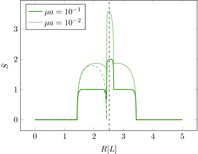
Figure 5: Entanglement entropy of vacuum fluctuations confined on a network idealised as a minimal star graph with three edges joined at a single vertex (referring to Fig. 3) in terms of the entangling sphere radius for two different values of $\mu a$. For comparison the entanglement entropy of vacuum fluctuations confined to a single edge with Dirichlet boundary conditions at both its endpoints is shown in dashed lines for both cases.

III.3 Infrastructure & Entanglement

Comparing the entanglement entropy of vacuum fluctuations confined to a minimal network with the corresponding quantum information measure on a single edge, both reported in Fig. 5, we observe deviations from the single edge configuration as the entangling sphere approaches the vertex of the minimal star graph. These deviations are triggered by correlations reaching from the interior edge across the vertex to the two edges residing outside the entangling sphere for both values of $\mu a$. As the entangling sphere is extended towards the vertex, the entanglement entropy of the minimal network increases relative to the single edge case, simply because more localised fluctuations per edge contribute to the entanglement. For lower values of $\mu a$ the effect is more pronounced due to the exponential decay of spatial correlations with $\mu a$ discussed above. In other words, a lower value of $\mu a$ implies a longer correlation length and, thus, an extended entanglement on larger network scales involving an increasing number of spatially separated fluctuations.

For $\mu a=10^{-1}$ the entanglement entropy for the single edge configuration develop a plateau which represents an upper bound on the entanglement entropy for the minimal network even as the entangling sphere approaches the vertex which opens up more communication channels. So despite the increase of correlations between the interior and the exterior of the entangling sphere, the entanglement entropy never exceeds the plateau value of the single edge configuration. This shows how the Kirchhoff-Neumann junction conditions control the impact of the vertex on the entanglement: The vertex decreases the strength of correlations across the junction by a factor $|E|^{-1}$ relative to the correlation strength between fluctuations localised sufficiently far away from it. Note that the entanglement entropy does, however, not vanish when the vertex intersects the surface of the entangling sphere.

A third effect of the network infrastructure on the entanglement of vacuum fluctuations confined to it concerns the presence of loops and is analysed in our code Giavoni et al. (2023), as well. Consider again the minimal network idealised as a star graph with three edges joining a single vertex, but now we connect two free endpoints and form a loop that is joined at the vertex by the single remaining edge, as indicated in Fig. 3 with the extension represented by the open polygon shown in green dashed lines. Loops in the infrastructure can counteract the impact of the vertex on the entanglement of vacuum fluctuations confined to the network. More precisely, if the entangling surface is close to the vertex, the presence of a loop can increase the entanglement entropy relative to the corresponding minimal graph configuration, provided the size of the loop is smaller than the typical correlation length. Then, loosely writing, the loop admits additional correlations between localised fluctuations inside and outside the entangling surface, respectively. If the loop size is larger than the typical correlation length, then, relative to the quantum information measure we used, the network configuration is effectively equivalent to the simple minimal network.

In conclusion, the entanglement entropy of vacuum fluctuations localised on more complicated networks constructed by joining several minimal networks is determined by the interplay of all the aforementioned effects. The following rule of thumb reflects the intuition supported by our numerical experiments: Each new edge intersecting the entangling surface adds more vacuum fluctuations that are correlated across the surface which leads to more entanglement, each new vertex sufficiently close to the entangling surface decreases the strength of correlations between vacuum fluctuations localised on different edges joined by this vertex, and each new loop of sufficiently small size (relative to the typical correlation length) further entangles the interior and exterior of the surface.

As a result, if the typical correlation length is large compared to the maximal size of any edge in a subgraph nested inside an idealised network, then the entanglement entropy of vacuum fluctuations measured by this part of the infrastructure will depend on its topology in addition to the number of its intersection with the entangling surface.

IV Area Scaling on Networks

The results of the previous section on the entanglement entropy of vacuum fluctuations confined to a minimal network – idealised as a star graph – which intersects a given entangling surface, can be used to deduce some entanglement properties of vacuum fluctuations on more sophisticated networks. Consider an arbitrary network, for instance the one depicted in gray in Fig. 3, and its intersection with the entangling surface (in this case a sphere). At each intersection point, the typical correlation length scale determines a sub-part of the graph, containing the intersection point, which we refer to as a local subgraph. A local subgraph either contains at least one vertex (connected to the intersection point), or it coincides with an entire edge or parts of it. If the correlation length is such that each local subgraph is disconnected from all the others (located at different intersection points), then, by our results from the previous section, we conclude right away that the entanglement entropy becomes, effectively, an extensive quantity relative to the disconnected local subgraphs,

$$S=\sum_{a\in\lceil n_{\mathrm{s}}\rfloor}S_{a}\;,$$ (21)

where $n_{\mathrm{s}}$ denotes the number of local subgraphs. The formula (21) for the total entanglement entropy holds, in particular, in the following situation: Suppose the correlation length satisfies the hierarchy $1/\mu\ll\mathrm{min}(l_{a},L_{a}-l_{a})$ for the edges in each subgraph on which the intersection points are located. Under the spell of this hierarchy the subgraphs effectively reduce to these edges when considering the entanglement entropy of a field with mass $\mu$, in accordance with the results of Sec. III.1. In this case all subgraphs become equivalent and the entanglement entropy is given by $S=n_{\mathrm{s}}\times S_{1}$. Again, this formula generalises the idea of Sec. III.1 to arbitrary networks upon identifying a single edge (on which the intersection point is located) with a disconnected subgraph. If the above hierarchy of length scale is inverted, then it is possible that vacuum fluctuations located in the neighbourhoods of different intersection points become correlated. In this case the entanglement entropy ceases to be an effectively extensive quantity and increases relative to the previous case.

We can elaborate the above findings further: If the typical correlation length of vacuum fluctuations confined to a network is smaller than the length scales characterising a given set of effectively disconnected (relative to the correlation length) subgraphs, each of which consists of connected components containing a single intersection point, then the entanglement entropy is an extensive quantity with respect to the disconnected subgraphs. Intuitively, the fluctuations cannot resolve the infrastructure beyond the individual subgraphs. In the extreme case that only the sizes of the subsystems on the intersected edge can be resolved, the entanglement entropy becomes maximally extensive in the sense that there is no smaller subgraph relative to which this property can hold. Relative to the same set of subgraphs, if the correlation length is increased, the vacuum fluctuation start to probe an increasing amount of facets of the network. At an intermediary step it might be possible to identify a new set of effectively disconnected subgraphs and establish an extensive entanglement entropy on larger scales. Relative to the extreme case discussed above, however, the entanglement entropy on each subgraph will depend on a complicated interplay of the effects discussed in Sec. III.3, albeit the characterisation as an extensive quantity relative to the subgraph level is valid. It is exactly in this regime that we leave the usual $1+1$ dimensional QFT treatment in favor of a full quantum graph description.

IV.1 Networks & Spacetime Entanglement

An exciting application of networks is as diagnostic devices to probe physical phenomena (compactly) supported in the embedding spacetime by solely employing fields confined to the networks and their two-dimensional piecewise smooth Lorentzian histories. This requires networks idealised by mesh-like graphs with compact extensions in all directions tangent to the instantaneous hypersurfaces in which they are at rest. Such an infrastructure naturally offers two types of investigations: The first concerns the similarity between physical systems confined to given networks and their counterparts enjoying compact but otherwise unrestricted spacetime support. Provided the similarity grows beyond experimental uncertainties, both systems cannot be discriminated (relative to the experiments), and the theory describing the system confined to the network and its two-dimensional histories can be considered a sufficient approximation of the (possibly ill-defined) continuum theory within the experimental accuracy. The second concerns employing networks adapted to probe aspects of the embedding spacetime geometry as captured by physical systems confined to the networks.

In field theory entanglement entropy becomes a continuum concept which is intrinsically dominated by short-distance correlations across the entangling surface. If the entangling surface is idealised as a border of infinitesimal width, and if it is wrongly assumed that details concerning a short-distance completion are irrelevant, then the entanglement entropy cannot be computed in quantum field theory. In other word, entanglement entropy as a quantity probing the spacetime continuum requires a short-distance completion. This seems to imply that entanglement entropy is not a meaningful quantum information measure in field theory. But this possibility is not enforced since even in the absence of a short-distance completion (intrinsic requirement), the definition of entanglement entropy can be adapted at the level of the infrastructure (extrinsic requirement). For instance, it is impossible to construct an infinitesimally thin entangling surface. Introducing a physical surface amounts necessarily to specifying a minimal distance scale. This is not done at the intrinsic level, since the surface is considered to be part and parcel of the hardware infrastructure which remains unresolved in terms of physical degrees of freedom. This is an example where any experiment comes automatically equipped with a finite resolution structure that we need to take into account at the operational level and that poses an extrinsic but at the same time principal resolution limit. So to offer a logical alternative it may be that we have to relax the formal definition of observables by taking into account finite resolution structure induced by an external object. Any measurement of entanglement entropy is performed relative to such a structure and this is inevitably unavoidable.

Our strategy in this section is to pursue the first investigation outlined above using entanglement entropy as a quantum information measure relative to a finite resolution structure for vacuum fluctuations in Minkowski spacetime, which simultaneously serves as a reference spacetime concerning the second type of investigations, that is, for probing generic spacetime geometries in which a network is embedded.

Concretely, we show in this section that a specific network class exists which allows to extract the entanglement entropy of vacuum fluctuations in the embedding Minkowski spacetime, albeit the network history is an embedded piecewise smooth two-dimensional Lorentzian history. This is an important example for emerging spacetime properties on lower dimensional structures. Let us stress again that the network does not serve as a discrete structure like a lattice, rather it comes equipped with a finite resolution structure. The network is a physical manifestation (hardware) of the support structure on which the physical degrees of freedom are bound to exist.

There are two reasons for a coarse-grained modeling of the continuum physics on the network. One is invited by the finite resolution structure itself and concerns the small-scale description of continuum quantities on the network. The other is the resolution of the embedding hypersurface (or spacetime) in terms of vertices. At each point in the interior of the edge there is a plane in the hypersurface tangent to the edge at this point. Only at the vertices can a path along the edge leave the local tangent plane in the hypersurface to extend in the remaining dimension. Thus the local vertex density can be used as a measure for the local filling of the hypersurface by the network. We choose a unit hypersurface volume to construct the local vertex density $d_{\mathrm{v}}$. The typical intrinsic reference scale is given by $\xi:=1/\mu$, where $\mu$ denotes the mass parameter of the vacuum fluctuations under considerations. This implies an effective intrinsic density scale for a coarse-grained description. Certainly, if the vertex density exceeds this scale, that is, if $d_{\mathrm{v}}\gg 1/\xi^{3}$, then fluctuations are blessed with ignorance concerning the coarse-grained (extrinsic) infrastructure they are confined to and probe the full embedding spacetime, subject only to the intrinsic resolution scale set by their mass parameter. Of course, this assumes that the vertex density $d_{\mathrm{v}}$ complies with the isometries of the embedding spacetime; in the case under consideration, $d_{\mathrm{v}}$ is assumed to be spacetime homogeneous to comply with the Poincaré isometry of Minkowski spacetime. Provided these two conditions are met, networks approximate the embedding spacetime, subject only to the intrinsic resolution limit of the fluctuations that are employed as spacetime probes. We refer to these networks as dense networks.

In the following we consider, for simplicity, a three-dimensional regular grid of finite size, where, in particular, all edges have the same length $L$. This network has one vertex per unit volume $L^{3}$, so $d_{\mathrm{v}}=1/L^{3}$. Hence the above relation between the intrinsic and extrinsic resolution scale becomes simply $L\ll\xi$.

We stress again that this network configuration must not be confused with a lattice, since contrary to the latter each of the network components support fluctuations on a two-dimensional Lorentzian submanifold embedded in a four-dimensional Minkowski spacetime. In other words, the fluctuations themselves act always as two-dimensional spacetime probes, contrary to field theory on a lattice where each nonempty vertex supports fluctuations that are sensitive to all spacetime dimensions.

For the following numerical experiments we refer the reader to the code Giavoni et al. (2023). Our discussion focuses on two regimes: One for which the entanglement entropy of vacuum fluctuations confined to a grid-like network is an extensive quantity relative to isolated subgraphs as discussed above, and the other for which the fluctuations probe the network on large scales so that the entanglement entropy manifests itself as an intensive quantity.

IV.1.1 Effectively extensive entanglement entropy

The discussion above implies that there is always a mass range of vacuum fluctuations for which the entanglement entropy of these fluctuations confined to a grid-like network is given by Eq. (21) relative to a given finite resolution structure. In the extreme case, $\xi\ll\min\{l_{\mathrm{e}},L-l_{\mathrm{e}}\}$ for each edge $\mathrm{e}$ containing a crossing point. This case corresponds effectively to a collapse of any choice of subgraphs connected to the entangling surface to a collection of edges piercing the entangling surface. In particular, the vertices cease to be the components controlling the spread of entanglement over the network. In other words, for this hierarchy between the typical internal and external distance scales, the ideal network description is reduced from graphs including vertices to just the edges piercing the entangling surface. Then, according to Eq. (21), the total entanglement entropy becomes effectively an extensive quantity given by $S=\mathcal{A}\times S_{1+1}$, where $\mathcal{A}$ is again the number of intersection points where the edges pierce the entangling surface. Due to the embedding of the network into Euclidean hypersurfaces geometrical information is available like the angle between the local normal of the entangling surface and the piercing edge. However, the vacuum fluctuations only probe the intrinsic edge geometry, or – if instead of an instantaneous network configuration a freely falling network is considered – the intrinsic geometry of the piecewise smooth Lorentzian network history. Nota bene, this is again because the fluctuations are not merely restricted but confined to the network and therefore cannot experience extrinsic geometry, which is why $S_{1+1}$ is independent of this information. As a consequence we may assume that all edges intersecting the entangling surface are aligned with the local normal, corresponding to a radial configuration in the case of an entangling sphere.

In the present subsection the entangling surface is considered to be spherical and thus, for each radius $R$ we obtain a finite collection of radial edges piercing the surface of the entangling sphere at an arbitrary location, depending on which network is concretely employed (or implemented in the numerical experiments). This leads, in general, to the number $\mathcal{A}$ of piercing points being some unknown function of the radius $R$. The analytical approach can substitute numerical experiments and is a suitable tool to diagnose, for instance, the entanglement properties of fields confined to freely falling networks in curved spacetimes, provided $\mathcal{A}(R)$ is known or can easily be modelled. As we will demonstrate further below, different network configurations and/or different shapes of regions containing degrees of freedom that we integrate out result in different values for $\mathcal{A}$.

Considering regular three-dimensional grid graphs with edges of length $L\ll R$, there is approximately one edge piercing the entangling surface per $L^{2}\pi/4$, leading to $\mathcal{A}(R)=16(R/L)^{2}$. The total entanglement entropy for such a configuration is given by $S(R)=\mathcal{A}(R)S_{1+1}(L/2)$. The calculation for an individual edge was outlined in Sec. III.1. Depending on the mass of the quantum field and on the length of the edges analytic expressions for $S_{1+1}(L/2)$ can be available. In Fig. 6, in green colour, we compare the analytical result $S(R)$, obtained by employing (25) for $S_{1+1}(L/2)$, to the numerical entanglement entropy. Note that numerically the surface area of the entangling sphere is overestimated by a factor of $4/\pi$, which we compensate for by multiplying the numerical entanglement entropy on these grid graphs with the inverse factor $\pi/4$, thus finding agreement to the case of a collection of radial edges with one puncture of the entangling sphere per $L^{2}$.

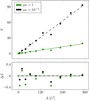
Figure 6: The upper plot shows the entanglement entropy $S_{\mathrm{grid}}$ of quantum fields in the ground state confined to a three-dimensional 11x11x11 regular grid graph with $11^{3}$ vertices and universal length $L=7a$ of the edges in terms of a minimal distance scale $a$ implied by an assumed finite resolution structure associated with some experiment. $S_{\mathrm{grid}}$ is shown in terms of the area $A$ of the entangling sphere. Data points correspond to numerical experiments for two different values of $\mu a$. For $\mu a=1$ (displayed in green colour), the analytical approximation $S(R)$ (green solid line) described in the main text is in good agreement with the data points (from numerical experiments). For the case $\mu a=10^{-3}$ (black data points) there is no analytical approximation for the given long-distance scale $L$. For convenience, a fit $S_{\mathrm{fit}}$ (black dashed lines) of the data from the numerical experiments has been added. The lower plot shows the quality of the agreement using $\Delta{S}=\delta S-1$ with $\delta S=S(R)/S_{\mathrm{grid}}$ for $\mu a=1$ and $\delta S=S_{\mathrm{fit}}/S_{\mathrm{grid}}$ for $\mu a=10^{-3}$.

The distance hierarchy $\xi=1/\mu\gg L$ lies outside the domain of validity of the analytical approach for obvious reasons: Under the spell of this hierarchy entanglement spreads over entire subgraphs of the network. As a consequence, in order to assess the entanglement of such a system, it is insufficient to analyse only the immediate neighbourhood of an entangling surface. This hierarchy then demands a numerical investigation of entanglement properties, and we employ again the code Giavoni et al. (2023) for a regular grid graph. For the results of our numerical experiment see Fig. 6, in black colour, and the figure caption for further details.

It is of fundamental importance that area scaling emerges in Fig. 6 for both hierarchies, $\xi=1/\mu\leq L$ and $\xi=1/\mu>L$, between the intrinsic and extrinsic distance scale characterising the total system. This is remarkable, because area scaling is a fingerprint for entangled fields extending in full spacetime, while we probe entanglement properties of fields confined to piecewise-smooth two-dimensional Lorentzian histories with instantaneous field configurations confined to edges of a given network.

Emerging spacetime properties of entanglement

In order to exploit this idea further, we investigate whether there is a class of networks serving as support structures for fields confined to them that allow to probe entanglement properties of the same type of fields extending in compact regions of Minkowski spacetime void of confining networks. In other words, we study the potential for spacetime entanglement emerging on piecewise smooth $(1+1)$-smooth Lorentzian histories.

As already mentioned, the proportionality factor between the entanglement entropy and the area of the entangling surface, for instance between the entanglement entropy and $4\pi R[L]^{2}$ shown in Fig. 6, depends on the specific network implemented in the (numerical) experiment. In fact, in order to obtain the same proportionality as for the entanglement entropy in $(1+3)$-dimensional Minkowski spacetime Srednicki (1993) with a given accuracy, the density of the idealised network in Minkowski spacetime has to be sufficiently high, entailing eventually the limit $L/R\rightarrow 0$ when the support of the fields confined to the network approximates a portion of the embedding four-dimensional Minkowski spacetime to arbitrary accuracy. This limit, however, cannot be achieved for the following reason: Before the short-distance cut-off below which the effective field theory requires a (partial) completion is reached, at the very least we know that our ignorance about the small-scale structure of spacetime in the semiclassical approximation has to be resolved eventually, the minimal distance scale $a$ implied by the finite resolution structure of any (numerical) experiment prohibits the required continuum limit. This is justified by any experiments, since networks represent physical hardware infrastructures that can be manufactured only with a finite density.

Alternatively, higher dimensional phenomena emerge if $L/\xi\ll 1$ and the network density exceeds one vertex per correlation length $\xi$ cubed. In this situation, the correlation length becomes too large to resolve the fine-grained network structures, that is, the entanglement properties become insensitive to the network details, which is why quantum fields confined to $(1+1)$-dimensional Lorentzian histories show an area scaling in their entanglement entropy.

In general, area scaling of the entanglement entropy is inevitable since massive degrees of freedom always allow to localise correlations in a neighbourhood containing the entangling surface. If the fields are not confined to a network but extend unrestricted to compact regions in spacetime, then they carry angular momentum, as well, which combines with their intrinsic mass to an effective mass. Even if the intrinsic mass vanishes, the angular momentum effectively limits entanglement to nearest neighbours (relative to some finite resolution structure) across the entangling surface Srednicki (1993). Thus area scaling is inevitable for the entanglement entropy of groundstate fluctuations in $(1+3)$-dimensional Minkowski spacetime.

However, fields confined to a network experience the intrinsic geometry of $(1+1)$-dimensional Lorentzian histories embedded in $(1+3)$-dimensional Minkowski spacetime with instantaneous field configurations confined to one-dimensional edges. Hence they do not carry angular momentum and the correlation length is solely determined by their intrinsic mass. Therefore, while an area law for $L\gg\xi$ could be expected because of the extensive property of the entanglement entropy in this regime (as seen by the green line in Fig. 6), it is very important that area scaling holds for $L\ll\xi$, as well (see the dashed black line in Fig. 6). This remains true even when correlations spread deep into the entangling sphere. In this situation correlations between fluctuations localised on different edges far apart (relative to the background geometry) still show area scaling of their entanglement entropy. This is only possible if the interplay of effects analysed in Sec. III.3 amounts to simulating the presence of angular momentum. In other words, we can interpret the results concerning the hierarchy $L\ll\xi$ shown in Fig. 6 as an emergence of angular momentum for the fields confined to the network which induces area scaling for their entanglement entropy. Therefore, networks equipped with fields confined to them are capable to trace fingerprints of the physics of these fields when they extend unrestricted (deconfined) to higher dimensional spacetime regions. Indeed, networks arise as potent arenas where phenomena experiencing all spacetime dimensions can be investigated using lower dimensional probes.

IV.2 Shape dependence

In this subsection we investigate entanglement of quantum graphs on the regular grid graph as in the previous subsection, but across an entangling surface of a different shape. Concretely, we trace over degrees of freedom located inside cubic regions of different volume, compute the respective entanglement entropies using our code Giavoni et al. (2023) and compare them to the case of entangling spheres. The entanglement entropy in terms of the area $A$ of the surface of the cube is shown in Fig. 7.

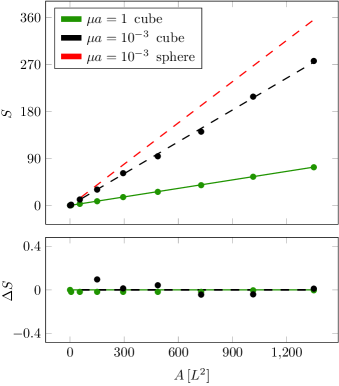
Figure 7: The upper plot shows the entanglement entropy $S_{\rm grid}$ of quantum fields in the ground state confined to a three-dimensional 17x17x17 regular grid graph with $17^{3}$ vertices and universal length $L=4a$ of the edges in terms of a minimal distance scale $a$ implied by an assumed finite resolution structure associated with some experiment. $S_{\mathrm{grid}}$ is shown in terms of the area $A$ of the entangling cube. Data points correspond to numerical experiments for two different values of $\mu a$. For $\mu a=1$ (displayed in green colour) the analytical approximation $S(R)$ is shown using a green solid line. A fit $S_{\mathrm{fit}}$ of the data for $\mu a=10^{-3}$ is depicted using a dashed black line. For comparison, the fit to the entanglement entropy for an entangling sphere introduced in Fig. 6 is shown in red. The lower plot shows the quality of the agreement using $\Delta{S}=\delta S-1$ with $\delta S=S(R)/S_{\mathrm{grid}}$ for $\mu a=1$ and $\delta S=S_{\mathrm{fit}}/S_{\mathrm{grid}}$ for $\mu a=10^{-3}$.

This result is a further concrete confirmation of the area law. It is worth noting that implementing an entangling cube yields data points scattered closer to a perfect area law, as compared to the case of an entangling sphere, and the dip observed in Fig. 6 for $A=180L^{2}$ is no longer present. This is because in the case we trace out a spherical region of a regular three dimensional grid, the entangling surface might intersect network vertices. As explained in Sec. III.3 for the case of a star graph with three edges, once the entangling surface resolves network vertices, the entanglement entropy is locally decreased and in the case of a grid graph even more since each vertex joins six edges. By tracing out a cubic region of a regular three dimensional grid network, it is possible to choose cube sizes such that vertices of the network remain unresolved.

Comparing the entanglement entropy results obtained by tracing out a sphere and a cube in Fig. 7 we find the following: Under the spell of the hierarchy $L\gg\xi$, the numerical experiments agree to very good precision on the value of the entanglement entropy $S(R)$ for the same areas of the entangling surfaces (where we note that for the cube the discrepancy to a perfect area law, i.e. $\Delta S$, is smaller compared to the one for the sphere). In fact, the analytically determined entanglement entropy given as a green line for the cube is identical to the one for the sphere. This is expected since the total entanglement entropy can be described by the entanglement entropy of fields confined to a collection of edges piercing the entangling shape, with one edge per unit surface area $L^{2}$. Since the entangling sphere and the cube are chosen to have the same area, the expectation follows. For the other hierarchy, $L\ll\xi$, the entanglement properties of fields confined to the network depend on the shape of the entangling surface. The reason is that under the spell of this hierarchy the entanglement is no longer restricted to locations within a neighbourhood of the entangling surface that just encompasses single edges across the surface. Instead degrees of freedom located deeper in the volume of the entangling surface get involved in entanglement across the surface which leads to the observed shape dependence, despite still providing an area scaling. In particular, Fig. 7 shows that the entanglement entropy related to an entangling sphere is larger than the one related to an entangling cube even if both entangling objects have the same surface area. It is interesting to speculate whether networks can be used to infer the shape of the entangling surface (not just its area). As a result, the network approach shows that, for $L\ll\xi$, the entanglement entropy of vacuum fluctuations confined on the network is not fully determined by the area of the traced out region, but also by its shape, with information about it encoded in the proportionality factor.

V Conclusions & Outlook

In this article, we presented a novel approach to investigate field theoretical phenomena by employing ideal networks equipped with fields confined to them, as diagnostic tools. As a first application, we have explored entanglement properties of quantum fields confined to networks histories embedded in the Minkowski background. Our findings show that although the fields are defined on $(1+1)$-dimensional Lorentzian histories with instantaneous field configurations localised on the one-dimensional edges of the network, the entanglement entropy scales with the area of the traced-out region, indicating the potential to explore nontrivial properties tight to the embedding $(1+3)$-dimensional spacetime.

As discussed with some of the authors of Tajik et al. (2023), experimentally there is the potential to measure the entanglement entropy in lab setups similar to network configurations discussed in this article, although technical limitations might restrict the complexity of the networks created. Alternative methods, like optical lattices, photonic integrated circuits or even materials like carbon nanotubes would offer more flexibility and allow for creating more complex networks. For example, quantum networks may also be realized in photon integrated circuits and hence give insights to their applications to optical quantum computers Andersen (2021), where, on a chip scale, squeezed states of light are feeded into an optical network consisting of several optical paths and beam splitters.

In the future, the increasing use of satellites with free space laser links for classical and quantum communication Toyoshima (2021); Liao et al. (2017) opens up new possibilities for quantum network experiments and potentially gravitational wave detection similar to large scale classical experiments like LISA Amaro-Seoane et al. (2017). Such networks build up by laser links as edges and satellites as vertices could be designed in various configurations, including fractal patterns inspired by fractal antennas in telecommunications with the advantage of having a high bandwidth and small size Werner and Ganguly (2003).

Throughout this article we presented graphs as an idealization of physical network structures on which quantum fields are confined. Extending this concept further, these networks might be thought as fundamental structures of nature itself. This perspective proposes a foundational role for $(1+1)$-dimensional physics, suggesting that $(1+3)$-dimensional physics could be an emergent phenomenon on quantum networks. Envisioning quantum networks as intrinsic to the fabric of the universe leads to a transformative approach to understanding physics. It implies that the complexities of our $(1+3)$-dimensional world might originate from simpler quantum processes within networks embedded in a four-dimensional spacetime. $(1+3)$-dimensional physics would then be an effective theory with an UV cutoff given by the typical edge length $L$. Physics beyond this cutoff would then not be dictated by $(1+3)$-dimensional physics but by its $(1+1)$-dimensional counterpart and additionally influenced by the network topology.

Our approach, when compared with other methods, reveals distinct advantages when considering problems in QFT in curved spacetimes. For instance, it allows the use of conformal methods, unlike $(1+3)$-dimensional lattice QFT. These unique characteristics make our approach a valuable alternative in the study of quantum fields. The relationship between different vacuum states in $(1+3)$-dimensions and those on the network is another intriguing aspect. Investigations into phenomena like black hole formation and Hawking radiation near event horizons, where particles experience extreme blue shifts, suggest that local studies using quantum networks could offer valuable insights.

Appendix A

A.1 Deconstructing the entanglement of continuous variable quantum systems

Perhaps naively entanglement entropy is an ill-defined information measure in quantum field theory. The qualification refers to the implicit assumption of a classical spacetime which allows for coincidence limits. In these limits entanglement entropy grows unbounded. Of course we do not know the structure of spacetime at arbitrary small scales. If entanglement entropy is a sensible concept in quantum field theory then something must prevent coincidence limits. On the other hand, events are measured to happen at places as opposed to points, but experiments assign to each place a point by way of error estimation in accordance with a given resolution limit. The latter induces a discrete localisation structure with a minimal distance scale given by devices employed in the measurement. This resolution limit is a fact and cannot be removed in our case. Within the given framework, the entanglement entropy of quantum systems described by continuous variables can only be quantified relative to an extrinsically given discrete localisation structure. The measurement device effectively maps continuous variable quantum systems to discrete quantum systems. We leave this investigation for future work.

In this appendix we focus on the extreme distance hierarchy $a\geq 1/\mu=\xi$, where $a$ denotes the extrinsically induced minimal distance scale. Under the spell of this hierarchy field configurations confined to graphs are transformed to systems of finitely many weakly coupled harmonic oscillators located on the edges of the graphs. Clearly, hierarchies of this type entail the entire span from the weak coupling regime to the decoupling limit, that is, the perturbative domain allowing to consider the Hamiltonian of the system as a small deviation from its diagonal part. In this perturbative framework the entanglement entropy Eq. (III.1) can be calculated analytically Riera and Latorre (2006); Katsinis and Pastras (2018).

Consider again the single edge depicted in red in Fig. 3 supporting a field configuration subjected to Dirichlet boundary conditions at its endpoints. Requiring that $a\gg 1/\mu$, instead of dealing with a continuous variable quantum system, the system reduces to a one-dimensional chain of finitely many, say $N$, harmonic oscillators. We assume that an entangling sphere intersects this edge dividing into an interior region containing $n$ oscillators and an exterior region where $N-n$ oscillators are located. In the interior and the exterior region the oscillators are equidistant from each other. Recall the form of the matrix $K$ given in Eq. (12),

$$K=M^{2}E+\Delta_{\mathrm{l}}\left(K\right)+\Delta_{\mathrm{u}}(K),$$ (22)

where $E$ denotes the $(N\times N)$ unit matrix, $M^{2}:=\tfrac{1}{N}\mathrm{tr}(K)=2+\mu^{2}a^{2}$, and the lower and upper triangular matrix is given by $(\Delta_{\mathrm{l}}(K))_{qs}=-\theta(N-s-1/2)\delta_{q,s+1}$ and $(\Delta_{\mathrm{u}}(K))_{qs}=-\theta(N-q-1/2)\delta_{q+1,s}$.

In the formal extreme distance hierarchy with $\mu a\gg 1$ the diagonal term $\mathrm{tr}(K)$ dominates over the off-diagonal terms since $\Delta_{\mathrm{l,u}}(K)$ are $\mu a$-independent. This allows to expand $\Omega=\sqrt{K}$ around its diagonal contribution Riera and Latorre (2006) with off-diagonals suppressed by inverse powers of $M$. The leading term in this expansion corresponds to the limit of decoupled oscillators characterised by a vanishing entanglement entropy. The onset of entanglement is encoded in the sub-leading terms

$$\Omega=M\,E-\tfrac{1}{2M}\,\left(\Delta_{\mathrm{l}}(K)+\Delta_{\mathrm{u}}(K)\right)+\mathcal{O}\left(\tfrac{1}{M^{3}}\right)\;.\,\,\,\,\,\,\,$$ (23)

In terms of the decomposition (15) of $\Omega$ into interior and exterior locations (relative to the entangling surface), we have $(\Omega_{\mathrm{II}})_{qs}=M\delta_{q,s}-\tfrac{1}{2M}(\delta_{q+1,s}+\delta_{q,s+1})+\mathcal{O}(M^{-3})$, with $q,s\in\lceil n\rfloor$. The coefficients of $\Omega_{\mathrm{EE}}$ have the same form but with indices in $\lceil N-n\rfloor$. Lastly, the submatrix $\Omega_{\mathrm{IE}}$ has a single nontrivial entry $-\tfrac{1}{2M}\delta_{u,n}\delta_{v,1}$ at leading order, with $u\in\lceil n\rfloor$, $v\in\lceil N-n\rfloor$, and $\Omega_{\mathrm{EI}}=(\Omega_{\mathrm{IE}})^{\mathrm{T}}$.

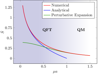
Figure 8: Entanglement entropy of degrees of freedom confined to a single edge that pierces the entangling surface at its midpoint as a function of $\mu a$. The length of the edge allows for $500$ oscillator locations equidistant from each other with separation $a$. This guarantees $\mu a\gg 0.002$ in the displayed domain $\mu a\in(0.05,1.5)$ so that finite size effects are not affecting the entanglement entropy evaluated at the midpoint of the edge. The red curve shows the numerical value obtained with the code Giavoni et al. (2023), while the blue and green curve, respectively, show $S^{\mathrm{plat}}$ and $S^{(3)}$ given in the main text. The background shading indicates the domain of validity of quantum field theory.

Since the submatrix $\Omega_{\mathrm{IE}}$ encodes the correlations between degrees of freedom located in the interior and exterior relative to the entangling surface, it is a zero matrix in the decoupling limit and therefore the entanglement entropy vanishes. The leading deviation from the decoupling limit is given by the $\mathcal{O}(1/M)$ contribution in the $1/M$ expansion. This contribution introduces a nearest neighbour correlation and, in particular, a correlation across the entangling surface between neighbouring oscillators that are located in the interior and exterior, respectively, relative to this surface. Taking only the leading deviation from the decoupling limit in the $1/M$ expansion into account, the onset of entanglement across the entangling surface can be quantified by a straightforward computation of the entanglement entropy up to and including the $\mathcal{O}(1/M)$ terms of the expansion.

If the entangling surface intersects an edge, the intersection contains a single point. In the leading deviation from the decoupling limit, only one communication channel between the nearest neighbours located on both sides of the surface can be established to support correlations across the surface. Solving the eigenvalue problem for $\gamma^{-1}\beta$ up to leading order Katsinis and Pastras (2018) in $1/M$ yields a single non-vanishing eigenvalue $\lambda={1}/{8M^{4}}$. Inserting $\lambda$ into Eq. (III.1) gives for the entanglement entropy

$$S^{(1)}=\frac{(1+4\ln(2M))}{16M^{4}}$$ (24)

at leading order in the expansion. Including the next to and next-to-next to leading order corrections Katsinis and Pastras (2018),

$${S}^{(3)}=S^{(1)}+\frac{1+328\ln(2M)}{512M^{8}}+\frac{-599+5880\ln(2M)}{3072M^{12}}\,.$$ (25)

As could have been anticipated from our numerical experiments, sufficiently close to the decoupling limit the entanglement entropy does not depend on the radius of the entangling sphere. In particular, for the threshold value $M=\sqrt{3}$, Eq. (25) agrees quantitatively to $97\%$ with the numerical value shown in Fig. 4. Moreover, for $M=\sqrt{3}$, entanglement across the entangling sphere is effectively restricted to configurations involving up to three correlated nearest neighbours. This agreement shows the validity (relative to the error) of the $1/M$ expansion even for the threshold value $M=\sqrt{3}$.

In Fig. 8 the entanglement entropy is depicted as a function of $\mu a$ for a single edge piercing the entangling sphere so that the puncture in the intersection coincides with the midpoint of the edge at $L/2$. The red curve represents the numerical value of the entanglement entropy. The blue curve shows the analytical result $S^{\mathrm{plat}}$ at $L/2$, as given in Calabrese and Cardy (2004). Finally, the green curve shows $S^{(3)}$ as given in Eq. (25). As can be seen, the plateau function $S^{\mathrm{plat}}$ evaluated at $L/2$ is a good approximation for values of $\mu a$ up to $0.2$ provided the distance hierarchy $L\gg 1/\mu=\xi$ holds. In Fig. 8 we chose $L=500a$ which implies a lower bound $\mu a\gg 0.002$. For values $\mu a>0.9$ the perturbative result $S^{(3)}$ is in good agreement with the numerical result. Between these regimes, that is for $0.2<\mu a<0.9$ no analytical approximation is available (to our knowledge).

The $1/M$ expansion can be applied to any graph configuration. For instance the loop configuration considered in Sec. III.1 and depicted in blue in Fig. 3. The ($N\times N$)-matrix $K$ (12) is adapted to accommodate periodic boundary conditions, which relative to a finite resolution structure are given by $\phi_{0}=\phi_{N}$ and $\phi_{N+1}=\phi_{1}$. In other words, $\phi_{1}$ and $\phi_{N}$ become nearest neighbours and will establish an additional robust communication channel in the $1/M$ expansion. This is the only difference compared to the single edge case, resulting in the following modification of the submatrix $\Omega_{\mathrm{IE}}$ of $\Omega=\sqrt{K}$: $(\Omega_{\mathrm{IE}})_{uv}=-\tfrac{1}{2M}(\delta_{u,n}\delta_{v,1}+\delta_{u,1}\delta_{v,N-n})$ to leading order in the $1/M$ expansion. Compared to the single edge case, the additional correlation supported by the second term in $\Omega_{\mathrm{IE}}$ implies an extra eigenvalue $\lambda=1/8M^{4}$ different from zero, giving, as expected, an additional contribution to the entanglement entropy of the loop configuration. Since this contribution does not depend on $n$, the entanglement entropy of the loop configuration is twice the entanglement entropy of the single edge (no loop) configuration, see Fig. 4 for $\mu a=1$.

References

- Berkolaiko and Kuchment (2012) G. Berkolaiko and P. Kuchment, Mathematical Surveys and Monographs (2012).
- Kottos and Smilansky (1997) T. Kottos and U. Smilansky, Phys. Rev. Lett. (1997).
- Kottos and Smilansky (2000) T. Kottos and U. Smilansky, Phys. Rev. Lett. (2000).
- Kostrykin and Schrader (1999) V. Kostrykin and R. Schrader, Journal of Physics A: Mathematical and General (1999).
- Fulling (2005) S. A. Fulling, “Local spectral density and vacuum energy near a quantum graph vertex,” (2005), arXiv:math/0508335 [math.SP] .
- Fulling et al. (2007) S. A. Fulling, L. Kaplan, and J. H. Wilson, Phys. Rev. A (2007).
- Schrader (2009) R. Schrader, Journal of Physics A: Mathematical and Theoretical 42, 495401 (2009).
- Bellazzini et al. (2008) B. Bellazzini, M. Burrello, M. Mintchev, and P. Sorba, (2008), 0801.2852 .
- Bellazzini and Mintchev (2006) B. Bellazzini and M. Mintchev, Journal of Physics A: Mathematical and General 39, 11101 (2006).
- Witten (2018) E. Witten, Reviews of Modern Physics (2018).
- Bombelli et al. (1986) L. Bombelli, R. K. Koul, J. Lee, and R. D. Sorkin, Phys. Rev. D 34, 373 (1986).
- Tajik et al. (2023) M. Tajik, I. Kukuljan, S. Sotiriadis, B. Rauer, T. Schweigler, F. Cataldini, J. Sabino, F. Møller, P. Schüttelkopf, S.-C. Ji, D. Sels, E. Demler, and J. Schmiedmayer, Nature Physics (2023).
- Srednicki (1993) M. Srednicki, Physical Review Letters 71, 666 (1993).
- Giavoni et al. (2023) C. Giavoni, S. Hofmann, and M. Koegler, “Emerging entanglement on network histories, https://doi.org/10.5281/zenodo.10437020,” (2023).
- Calabrese and Cardy (2004) P. Calabrese and J. Cardy, Journal of Statistical Mechanics: Theory and Experiment 2004 (2004).
- Andersen (2021) U. L. Andersen, Nature (2021).
- Toyoshima (2021) M. Toyoshima, Journal of Lightwave Technology 39, 693 (2021).
- Liao et al. (2017) S.-K. Liao et al., Nature 549, 43 (2017).
- Amaro-Seoane et al. (2017) P. Amaro-Seoane et al. (LISA), (2017), arXiv:1702.00786 [astro-ph.IM] .
- Werner and Ganguly (2003) D. H. Werner and S. Ganguly, IEEE Antennas and propagation Magazine 45, 38 (2003).
- Riera and Latorre (2006) A. Riera and J. Latorre, Physical Review A 74 (2006), 10.1103/PHYSREVA.74.052326.
- Katsinis and Pastras (2018) D. Katsinis and G. Pastras, The European Physical Journal C 78, 1 (2018).