CP-Violating Axions: A Theory Review

Abstract

We review the physics case for CP-violating axions. In the first part, we focus on the Quantum Chromodynamics (QCD) axion and argue that new sources of CP violation beyond QCD misalign the axion solution to the strong CP problem and can manifest themselves via a tiny scalar axion-nucleon component. We hence highlight recent advancements in calculating this scalar axion-nucleon coupling, a parameter that could be probed via axion-mediated force experiments. In the second part, we focus on axion-like particle (ALP) interactions entailing the most general sources of CP violation. After classifying the full set of CP-violating Jarlskog invariants, we report on recent calculations of ALP contributions to permanent electric dipole moments. We finally speculate on possible ultraviolet completions of the CP-violating ALP.

1 Introduction

Among light and weakly coupled new physics scenarios beyond the Standard Model (SM), the Quantum Chromodynamics (QCD) axion stands out as a most compelling paradigm, by simultaneously providing an elegant solution to the strong CP problem via the Peccei Quinn (PQ) mechanism ^{1, 2, 3, 4} and an excellent dark matter candidate ^{5, 6, 7}. The experimental landscape for axion searches has considerably broadened in the recent years, see ^{8, 9} for recent reviews. While traditional axion searches target the standard axion-photon coupling, novel detection strategies have been also proposed to probe axion couplings to nucleons ^{10, 11, 12, 13, 14} and electrons ^{15, 16, 17, 18}. These are especially relevant in view of their complementarity in disentangling different realizations of QCD axion models. Other low-energy signatures of QCD axions could stem from flavour- and CP-violating processes. Indeed, although negligible in benchmark axion models ^{19, 20, 21, 22}, sizeable flavour- and CP-violating axion couplings may be naturally generated in non-minimal scenarios addressing the SM flavour puzzle ^{23, 24, 25, 26, 27, 28} and/or accounting for the observed matter-antimatter asymmetry of the universe.

Standard QCD axion models predict a strict relation between the axion mass and its decay constant, enforcing an upper bound on the axion mass of about 0.1 eV after imposing astrophysical and cosmological bounds. Instead, in the more general framework of axion-like particles (ALPs), such a stringent condition is relaxed and much larger ALP masses can be conceived. ALP interactions with SM fermions and gauge bosons are then described via an effective Lagrangian containing operators up to $d=5$ ²⁹. The opportunity to look for ALPs with masses above the MeV scale, whose couplings are not tightly constrained by astrophysical bounds, opens the possibility to probe ALP interactions via collider searches ^{30, 31, 32, 33, 34, 35, 36, 37, 38, 39} and flavour-violating observables, both in the quark ^{40, 41, 42, 43, 44, 45, 46} and in the lepton sectors ^{47, 48, 49}.

Conversely, CP-violating observables involving either QCD axions or ALPs have received relatively less attention. It is hence the purpose of this review to summarize the physics case for CP-violating axions. In the case of QCD axions, this is addressed by providing the basic ingredients behind the origin of CP-violating axion couplings, and by reporting on recent calculations of CP-violating couplings to nucleons. Instead, in the case of ALPs, we discuss the most general CP-violating ALP interactions, both for ALP masses above few GeV, where QCD can be treated perturbatively, and below the GeV scale, where non-perturbative methods such as chiral perturbation theory ($\chi$pt) are mandatory. The impact on electric dipole moments (EDMs) is discussed in both regimes.

The experimental prospects for probing CP-violating axion interactions via axion-mediated force experiments and future improvements in the measurements of permanent EDMs of nucleons, nuclei, atoms and molecules will be also reviewed. The review is structured around two main parts, discussing respectively the case of CP-violating QCD axions (Sect. 2) and CP-violating ALPs (Sect. 3).

2 CP-violating QCD axions

The QCD axion originally emerged from the need to “wash out” CP violation from strong interactions ^{1, 2, 3, 4}. From an effective field theory (EFT) perspective, the PQ solution to the strong CP problem can be formulated as follows. The SM Lagrangian is augmented by a spin-0 field $a(x)$ endowed with a pseudo-shift symmetry, $a\to a+\alpha f_{a}$, that is broken only by the operator

$$\frac{a}{f_{a}}\frac{\alpha_{s}}{8\pi}G\tilde{G}~{},$$ (1)

with $G\tilde{G}\equiv\frac{1}{2}\epsilon^{\mu\nu\rho\sigma}G^{a}_{\mu\nu}G^{a}_{\rho\sigma}$. After employing the pseudo-shift symmetry to reabsorb the QCD $\theta$ term by setting $\alpha=-\theta$, one is left in the shifted theory with the operator in Eq. (1). Hence, the question of CP violation in strong interactions is traded for a dynamical question about the vacuum expectation value (VEV) of the axion field

$$\theta_{\rm eff}\equiv\frac{\left\langle a\right\rangle}{f_{a}}~{},$$ (2)

resulting into an effective $\theta$ parameter, with $|\theta_{\rm eff}|\lesssim 10^{-10}$ from the non-observation of the neutron EDM (nEDM) ^{50, 51}.

A general result, due to Vafa and Witten ⁵², ensures that the ground state energy density of QCD ${\cal E}$ is minimized for $\theta_{\rm eff}=0$, namely ${\cal E}(0)\leq{\cal E}(\theta_{\rm eff})$. The argument is based on an inequality that exploits the path-integral representation of ${\cal E}$ ⁵³. At large 4-volume in Euclidean space, one has

$$e^{-V_{4}{\cal E}(\theta_{\rm eff})} =\int\mathcal{D}\varphi e^{-S_{0}+i\theta_{\rm eff}{\cal Q}}=\Big{|}\int\mathcal{D}\varphi e^{-S_{0}+i\theta_{\rm eff}{\cal Q}}\Big{|}$$

$$\leq\int\mathcal{D}\varphi\Big{|}e^{-S_{0}+i\theta_{\rm eff}{\cal Q}}\Big{|}=e^{-V_{4}{\cal E}(0)}~{},$$ (3)

where $\varphi$ denotes the collection of QCD fields (quarks and gluons), $S_{0}$ is the QCD Lagrangian in absence of the $\theta$ term and we introduced the topological charge operator ${\cal Q}\equiv\int d^{4}x\frac{\alpha_{s}}{8\pi}G\tilde{G}$, which takes integer values in the background of QCD instantons. A crucial assumption, on which the proof in Eq. (2) relies, consists in the positive definiteness of the path-integral measure

$$\mathcal{D}\varphi\equiv\mathcal{D}A^{a}_{\mu}~{}\mbox{det}\,(\not{D}+M)~{},$$ (4)

where the Gaussian path-integral over the fermionic fields has been explicitly performed. However, while the fermionic determinant is positive definite in a vector-like theory such as QCD, this is not the case for a chiral theory like the SM. Hence, we cannot apply the Vafa-Witten theorem to the SM, although the argument does not automatically imply that $\theta_{\rm eff}\neq 0$ in the SM. An extra ingredient of the SM is that CP is explicitly broken in the quark sector by the Cabibbo-Kobayashi-Maskawa (CKM) phase, which is responsible for a $\theta_{\rm eff}\neq 0$ term.

2.1 The QCD axion ground state in the presence of CP violation

Given a short-distance CP-violating local operator $\mathcal{O}_{\rm CPV}(x)$, we can estimate the value of $\theta_{\rm eff}$ by expanding the axion potential as

$$V(\theta_{\rm eff})=K^{\prime}\theta_{\rm eff}+\frac{1}{2}K\theta_{\rm eff}^{2}+\mathcal{O}(\theta^{3}_{\rm eff})~{},$$ (5)

and focus on the $\theta_{\rm eff}\ll 1$ regime, since we know that $|\theta_{\rm eff}|\lesssim 10^{-10}$. Here, $K$ is a 2-point function also known as topological susceptibility ²⁰

$$K=i\int d^{4}x\langle 0|\mathcal{T}\frac{\alpha_{s}}{8\pi}G\tilde{G}(x)\frac{\alpha_{s}}{8\pi}G\tilde{G}(0)|0\rangle~{},$$ (6)

where $\mathcal{T}$ denotes the time-ordered product. This quantity is related to the axion mass via $K=m_{a}^{2}f_{a}^{2}$, while $K^{\prime}$ is a 1-point function given by ⁵⁵

$$K^{\prime}=i\int d^{4}x\langle 0|\mathcal{T}\frac{\alpha_{s}}{8\pi}G\tilde{G}(x)\mathcal{O}_{{\rm CPV}}(0)|0\rangle~{}.$$ (7)

Note that $K^{\prime}\neq 0$ because $G\tilde{G}$ and $\mathcal{O}_{{\rm CPV}}$ are both CP-odd, and CP-violating effects can be safely neglected for the evaluation of the QCD matrix element. The induced $\theta_{\rm eff}$ is hence obtained via the direct minimization of $V(\theta_{\rm eff})$ in Eq. (5), yielding

$$\theta_{\rm eff}\simeq-\frac{K^{\prime}}{K}~{}.$$ (8)

The value of $\theta_{\rm eff}$ in the SM was estimated by Georgi and Randall in Ref. ⁵⁶. At energies below $\Lambda_{\chi}=4\pi f_{\pi}$ with $f_{\pi}\simeq 92$ MeV one can write a flavour conserving, CP-violating operator

$$\mathcal{O}^{\rm SM}_{\rm CPV}=\frac{G_{F}^{2}}{m_{c}^{2}}J_{\rm CKM}[\overline{u}\gamma^{\mu}(1-\gamma_{5})d\cdot\overline{d}\gamma_{\mu}]\not{D}[\gamma^{\nu}(1-\gamma_{5})s\cdot\overline{s}\gamma_{\nu}(1-\gamma_{5})u]~{},$$ (9)

which is obtained in the SM after integrating out the $W$ boson and the charm quark (see diagram in Fig. 1 of ⁵⁶), while $J_{\rm CKM}=\mbox{Im}\,V_{ud}V^{*}_{cd}V_{cs}V^{*}_{us}\simeq 3\times 10^{-5}$ is the reduced Jarlskog invariant ⁵⁷. A proper evaluation of the $K^{\prime}$ matrix element in the presence of $\mathcal{O}^{\rm SM}_{\rm CPV}$ is a non-trivial task. However, by the rules of naive dimensional analysis (NDA) ⁵⁸ one expects $K^{\prime}\sim f_{\pi}^{4}\frac{G_{F}^{2}}{m_{c}^{2}}J_{\rm CKM}f_{\pi}^{4}\Lambda^{2}_{\chi}$ ⁵⁶. Hence, taking also $K\sim f_{\pi}^{4}$ (indeed, $K\simeq(76\ \text{MeV})^{4}$ – see ^{60, 61}), one obtains

$$\theta^{\rm SM}_{\rm eff}\sim\frac{G_{F}^{2}}{m_{c}^{2}}J_{\rm CKM}f_{\pi}^{4}\Lambda^{2}_{\chi}\sim 10^{-19}~{},$$ (10)

which should be taken as an indicative estimate of the CKM contribution.

It is interesting to note that the PQ mechanism would have been ineffective in a modified SM with the QCD and the Fermi scales closer to each other and/or in the presence of a trivial flavour structure such that $J_{\rm CKM}\sim 1$. Also, the PQ mechanism is not generically going to work in a low-scale theory beyond the SM with generic CP violation. To see this, assume a $d=6$ CP-violating operator $\mathcal{O}_{\rm CPV}/\Lambda_{\rm BSM}^{2}$, coupled to QCD. Following an estimate similar to that in Eq. (10) one obtains

$$\theta^{\rm BSM}_{\rm eff}\sim\left(\frac{\Lambda_{\chi}}{\Lambda_{\rm BSM}}\right)^{2}\sim 10^{-10}\left(\frac{100\ \text{TeV}}{\Lambda_{\rm BSM}}\right)^{2}~{},$$ (11)

where in the second step we have normalized $\theta^{\rm BSM}_{\rm eff}$ to the bound set by the nEDM. This expression suggests that the QCD axion could act as a low-energy probe of high-energy sources of CP-violation, by testing generic CP-violating new physics up to the scale $\Lambda_{\rm BSM}\lesssim 100$ TeV.

An axion VEV could also be generated from an ultraviolet (UV) source of PQ breaking that is not aligned to the QCD anomaly. This is motivated by the fact that the U(1)_PQ, being a global symmetry, does not need to be exact and it is expected to be broken by quantum gravity effects (see e.g. ⁶²). Hence, the axion VEV could be displaced from zero, leading to the so-called PQ quality problem ^{63, 64, 65}, that is the need to explain why UV physics does not generically spoil the QCD axion solution to the strong CP problem. There actually exist UV constructions, based e.g. on extra gauge symmetries (see e.g. ^{66, 67, 68, 69, 70, 71, 72, 73, 74, 75, 76}), which ensure a controlled solution to the PQ quality problem. In the following, we will assume as a canonical example a PQ-breaking effective operator of the type

$$V_{\text{PQ-break}}=e^{i\delta_{\theta}}\frac{\Phi^{n}}{\Lambda_{\rm UV}^{n-4}}+\text{h.c.}~{},$$ (12)

with $n>4$. Here, $\delta_{\theta}$ denotes a generic phase, $\Lambda_{\rm UV}$ is some UV scale like the Planck mass and $\Phi=\frac{f_{a}}{\sqrt{2}}e^{i\theta}$ is a complex scalar, with the radial mode integrated out and the angular mode $\theta=a/f_{a}$ given by the axion. In terms of $\theta$, the PQ-breaking potential reads

$$V_{\text{PQ-break}}=\frac{1}{2^{n/2-1}}\frac{f_{a}^{n}}{\Lambda_{\rm UV}^{n-4}}\cos(n\theta+\delta_{\theta})~{}.$$ (13)

In general, the phase of this potential, parameterized by $\delta_{\theta}$, needs not be aligned with the CP-conserving minimum of the QCD potential at $\theta=0$. Therefore, we generically expect $\delta_{\theta}$ to be $\mathcal{O}(1)$. The balance between $V_{\rm PQ-break}$ and the standard QCD axion potential, $V_{\rm QCD}=\frac{1}{2}f_{a}^{2}m_{a}^{2}\theta^{2}+\mathcal{O}(\theta^{4})$, yields the axion VEV (approximated for $\theta\ll 1$)

$$\theta_{\rm eff}\simeq-\frac{n\Lambda_{\rm UV}^{4-n}f_{a}^{n}\sin\delta_{\theta}}{2^{\frac{n}{2}-1}f_{a}^{2}m_{a}^{2}}~{},$$ (14)

which effectively also breaks CP. Taking for instance $\sin\delta_{\theta}=1$, $\Lambda_{\rm UV}=M_{\rm Pl}$ and $f_{a}=10^{8}$ GeV, the nEDM bound $|\theta_{\rm eff}|\lesssim 10^{-10}$ translates into $n\geq 9$.

While the nEDM directly probes $\theta_{\rm eff}$, the presence of a propagating light axion field could offer additional ways to test the axion ground state, as discussed in the following.

2.2 CP-violating axion-nucleon couplings

A remarkable consequence of $\theta_{\rm eff}\neq 0$ is the generation of a scalar axion coupling to nucleons, $g^{S}_{aN}a\overline{N}N$ (with $N=p,n$), which can be searched for in axion-mediated force experiments as suggested by Moody and Wilczek ⁷⁷. The phenomenological relevance of these observables will be discussed in Sect. 2.3. To understand the origin of $g^{S}_{aN}$, let us define the canonical axion field as the excitation over its VEV, $a\to\theta_{\rm eff}f_{a}+a$, and consider the two-flavour QCD axion Lagrangian

$$\mathcal{L}_{a}=\frac{\alpha_{s}}{8\pi}\left(\theta_{\rm eff}+\frac{a}{f_{a}}\right)G\tilde{G}-\overline{q}_{L}M_{q}q_{R}+\text{h.c.}~{},$$ (15)

where $M_{q}=\mbox{diag}\,(m_{u},m_{d})$. Upon the quark field redefinition

$$q\to e^{\frac{i}{2}\gamma_{5}\left(\theta_{\rm eff}+\frac{a}{f_{a}}\right)Q_{a}}q~{},$$ (16)

with $Q_{a}=M_{q}^{-1}/\mbox{Tr}\,M_{q}^{-1}=\mbox{diag}\,(\frac{m_{d}}{m_{u}+m_{d}},\frac{m_{u}}{m_{u}+m_{d}})$, the $G\tilde{G}$ term in Eq. (15) gets rotated away, while the quark mass matrix becomes

$$M_{q}\to M_{a}=e^{i\gamma_{5}\left(\theta_{\rm eff}+\frac{a}{f_{a}}\right)Q_{a}}M_{q}~{},$$ (17)

where we used $[M_{q},Q_{a}]=0$. Hence, in the new basis we have

$$\mathcal{L}_{a} =-\overline{q}\left[\frac{M_{a}+M^{\dagger}_{a}}{2}+\gamma_{5}\frac{M_{a}-M^{\dagger}_{a}}{2}\right]q$$

$$=-\overline{q}\cos\left(\left(\theta_{\rm eff}+\frac{a}{f_{a}}\right)Q_{a}\right)M_{q}q-\overline{q}i\gamma_{5}\sin\left(\left(\theta_{\rm eff}+\frac{a}{f_{a}}\right)Q_{a}\right)M_{q}q~{}.$$ (18)

Focusing on the scalar component (i.e. the term without $\gamma_{5}$)

$$\mathcal{L}_{a} \supset-\overline{q}\cos\left(\theta_{\rm eff}Q_{a}\right)\cos\left(\frac{a}{f_{a}}Q_{a}\right)M_{q}q+\overline{q}\sin\left(\theta_{\rm eff}Q_{a}\right)\sin\left(\frac{a}{f_{a}}Q_{a}\right)M_{q}q$$

$$\simeq\theta_{\rm eff}\frac{a}{f_{a}}\overline{q}~{}Q_{a}^{2}M_{q}q=\frac{\theta_{\rm eff}}{f_{a}}\frac{m_{u}m_{d}}{m_{u}+m_{d}}a\left(\frac{m_{d}}{m_{u}+m_{d}}\overline{u}u+\frac{m_{u}}{m_{u}+m_{d}}\overline{d}d\right)~{},$$ (19)

where in the second step we kept only a term linear in $a/f_{a}$ and expanded for small $\theta_{\rm eff}$, while in the last step we employed the explicit representation of $Q_{a}$ given below Eq. (16). Hence, the scalar axion coupling to nucleons is

$$g^{S}_{aN} =\frac{\theta_{\rm eff}}{f_{a}}\frac{m_{u}m_{d}}{m_{u}+m_{d}}\left(\frac{m_{d}}{m_{u}+m_{d}}\langle N|\overline{u}u|N\rangle+\frac{m_{u}}{m_{u}+m_{d}}\langle N|\overline{d}d|N\rangle\right)$$ (20)

$$=\frac{\theta_{\rm eff}}{f_{a}}\frac{m_{u}m_{d}}{m_{u}+m_{d}}\left[\frac{\langle N|\overline{u}u+\overline{d}d|N\rangle}{2}+\left(\frac{m_{d}-m_{u}}{m_{u}+m_{d}}\right)\frac{\langle N|\overline{u}u-\overline{d}d|N\rangle}{2}\right]~{},$$

where in the last step we isolated the iso-spin singlet component, $\overline{u}u+\overline{d}d$. Focusing on the leading iso-spin singlet term (as in ⁷⁷), one has

$$g^{S}_{aN}\simeq\frac{\theta_{\rm eff}}{f_{a}}\frac{m_{u}m_{d}}{m_{u}+m_{d}}\frac{\langle N|\overline{u}u+\overline{d}d|N\rangle}{2}\simeq 1.3\cdot 10^{-12}~{}\theta_{\rm eff}\left(\frac{10^{10}\ \text{GeV}}{f_{a}}\right)~{}.$$ (21)

For the numerical evaluation, we employed the value of the pion-nucleon sigma term $\sigma_{\pi N}=\langle N|\overline{u}u+\overline{d}d|N\rangle(m_{u}+m_{d})/2=59.1\pm 3.5$ MeV ⁷⁸. As pointed out in Ref. ⁷⁹, a factor $1/2$ was missed in the original derivation of Moody and Wilczek ⁷⁷.

Note that Eq. (21) is formally correct only in the case in which the origin of the axion VEV is due to a UV source of PQ breaking, as e.g. in Eq. (12). On the other hand, in the more general case of CP-violating sources related to QCD, i.e. a short distance operator made of quarks and gluons, Eq. (21) turns out to be conceptually unsatisfactory when we focus on the relevant question: how to properly correlate the scalar axion-nucleon coupling with the nEDM bound? The reason being the Eq. (21) misses extra contributions due to meson tadpoles ($\pi^{0}$, $\eta$, $\eta^{\prime}$), which are generated by the same UV source of CP violation responsible for $\theta_{\rm eff}\neq 0$ and are of the same size of the term proportional to $\theta_{\rm eff}$. This improvement was recently taken into account in Ref. ⁷⁹ which, including as well iso-spin breaking effects from the leading order axion-baryon-meson chiral Lagrangian, found the master formula

$${g}^{S}_{an,\,p} \simeq\frac{4B_{0}\,m_{u}m_{d}}{f_{a}(m_{u}+m_{d})}\bigg{[}\pm(b_{D}+b_{F})\frac{\left\langle\pi^{0}\right\rangle}{F_{\pi}}+\frac{b_{D}-3b_{F}}{\sqrt{3}}\frac{\left\langle\eta_{8}\right\rangle}{F_{\pi}}-\sqrt{\frac{2}{3}}(3b_{0}+2b_{D})\frac{\left\langle\eta_{0}\right\rangle}{F_{\pi}}$$

$$-\left(b_{0}+(b_{D}+b_{F})\frac{m_{u,d}}{m_{d}+m_{u}}\right)\theta_{\rm eff}\bigg{]}~{},$$ (22)

where for clarity we neglected $m_{u,d}/m_{s}$ terms. Here, $B_{0}=m_{\pi}^{2}/(m_{d}+m_{u})$ while the hadronic Lagrangian parameters $b_{D,F}$ are determined from the baryon octet mass splittings, $b_{D}\simeq 0.07\,\rm GeV^{-1}$, $b_{F}\simeq-0.21\,\rm GeV^{-1}$ at LO ⁸⁰. The value of $b_{0}$ is determined from the pion-nucleon sigma term as $b_{0}\simeq-\sigma_{\pi N}/4m_{\pi}^{2}$. From the determination in ⁷⁸ one obtains $b_{0}\simeq-0.76\pm 0.04\,\rm GeV^{-1}$. Given $\sigma_{\pi N}\equiv\langle N|\overline{u}u+\overline{d}d|N\rangle\,(m_{u}+m_{d})/2$, the isospin symmetric $b_{0}\theta_{\rm eff}$ term reproduces exactly Eq. (21).

In general, $g^{S}_{aN}$ and $d_{n}$ are not proportional, as it would follow instead from Eq. (21). For instance, exact cancellations among the VEVs can happen for $d_{n}$ ^{81, 82} which have no counterpart in $g^{S}_{aN}$. Note that $\theta_{\rm eff}$ and the meson VEVs in Eq. (2.2) are meant to be computed from high-energy sources of CP violation, represented by an effective operator $\mathcal{O}_{\rm CPV}$. In Ref. ⁷⁹ an explicit example was worked out in the context of 4-quark operators of the type $\mathcal{O}_{\rm CPV}=(\overline{q}q)(\overline{q}^{\prime}i\gamma_{5}q^{\prime})$ with $q,q^{\prime}=u,d,s$, arising e.g. by integrating out the heavy $W_{R}$ boson in left-right symmetric models. Building on the detailed analysis of Ref. ⁸², both $g^{S}_{aN}$ and $d_{n}$ were computed in the minimal left-right symmetric model with $\mathcal{P}$-parity ^{83, 84}, showing a non-trivial interplay which deviates sizeably from the naive scaling implied by Eq. (21), that is $g^{S}_{aN}\propto d_{n}\propto\theta_{\rm eff}$.

More recent works have readdressed the calculation of $g^{S}_{aN}$ in terms of short-distance sources of CP violation. Ref. ⁸⁵ considered the contribution of EDMs and color EDMs of quarks, and revisited as well the SM contribution arising from the CKM phase. Ref. ⁸⁶ provided instead a systematic calculation of CP-violating axion couplings, starting from the CP-violating basis of low-energy EFT (LEFT) operators of quarks and gluons, and employing at low-energy a chiral Lagrangian approach, similar to the one of Eq. (2.2).

2.3 Axion-mediated forces vs nEDM

Including both scalar and pseudo-scalar couplings to matter fields, the axion interaction Lagrangian can be written as

$$\mathcal{L}^{\rm int}_{a}\supset g^{S}_{aN}a\overline{N}N+g^{P}_{af}a\overline{f}i\gamma_{5}f~{},$$ (23)

where $f=N,e$, and $g^{P}_{af}=C_{f}m_{f}/f_{a}$ denoting the usual pseudo-scalar axion coupling, with $C_{f}\sim\mathcal{O}(1)$ in benchmark axion models ⁸⁷.

By taking the non-relativistic limit of $\mathcal{L}^{\rm int}_{a}$ one obtains different kinds of static potentials, which can manifest themselves as new axion-mediated macroscopic forces ⁷⁷. The latter can be tested in laboratory experiments, and hence do not rely on model-dependent axion production mechanisms, as in the case of dark matter axions (haloscopes) or to a lesser extent solar axions (helioscopes). An updated review of axion-mediated force experiments and relevant limits can be found in Ref. ⁸⁸ (see also ^{89, 8, 9}).

Axion-induced potentials can be of three types, depending on the combination of couplings involved, i.e. $g^{S}_{aN}g^{S}_{af}$ (monopole-monopole), $g^{S}_{aN}g^{P}_{af}$ (monopole-dipole) and $g^{P}_{af}g^{P}_{af}$ (dipole-dipole). The idea of searching for dipole-dipole axion interactions in atomic physics is as old as the axion itself ³. However, dipole-dipole forces turn out to be spin suppressed in the non-relativistic limit and suffer from large backgrounds from ordinary magnetic forces. Searches based on monopole-monopole interactions, like tests of gravity on macroscopic scales, are in principle much more powerful. However, under the theoretical prejudice that we are after the QCD axion, the $\theta_{\rm eff}^{2}$ suppression (given the nEDM bound) is such that current experiments are still some orders of magnitude away from testing the QCD axion.

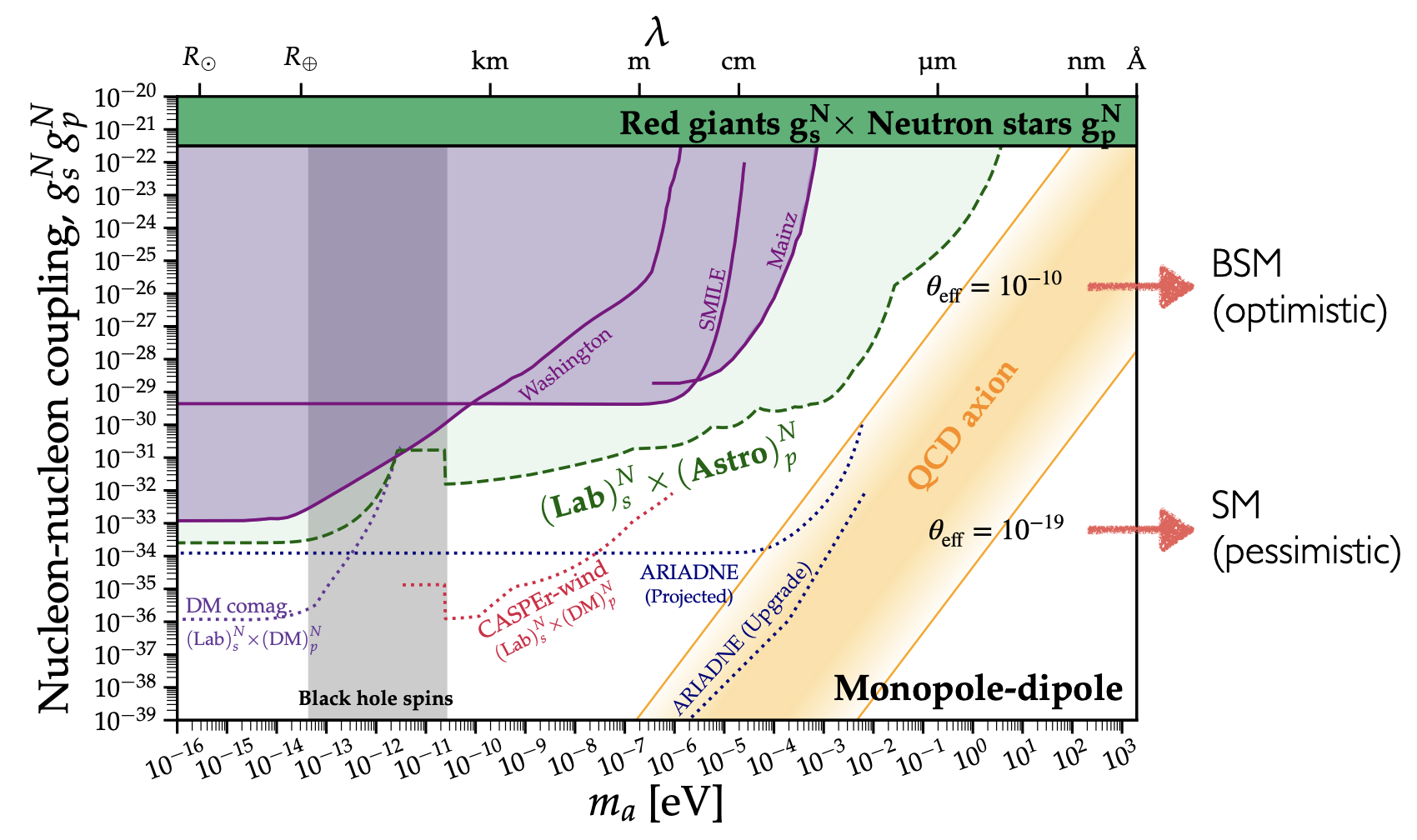
Figure 1: Parameter space of axion-mediated monopole-dipole forces. Figure adapted from Ref. ⁸⁸.

The sweet spot is given by monopole-dipole searches which, as shown in Fig. 1, will enter into the QCD axion region. In this case, the axion-mediated potential between nucleons and a spin sample of fermions of type $f$ is given by ⁷⁷

$$V(r)=g^{S}_{aN}g^{P}_{af}\frac{\hat{\sigma}\cdot\hat{r}}{8\pi M_{f}}\left(\frac{m_{a}}{r}+\frac{1}{r^{2}}\right)e^{-m_{a}r}~{},$$ (24)

which implies that for $m_{a}r\lesssim 1$, so that the potential is not exponentially suppressed, $V(r)$ falls like $1/r^{2}$. A new detection concept by the ARIADNE collaboration ^{12, 13} plans to use nuclear magnetic resonance techniques to probe the axion field sourced by an unpolarized material via a sample of nucleon spins. Note that the yellow QCD axion band in Fig. 1 is obtained by employing Eq. (21) for the scalar axion-nucleon coupling, with the value of $\theta_{\rm eff}$ spanning from the SM estimate $\theta_{\rm eff}\sim 10^{-19}$ (lower side) to the limit imposed by the nEDM $\theta_{\rm eff}\simeq 10^{-10}$ (upper side). However, as argued in Sect. 2.2, the relation between $g^{S}_{aN}$ and $d_{n}$ is model dependent and hence, given a specific source of CP-violation, it should be assessed case by case in order to properly determine the parameter space region that is allowed by the nEDM bound (for a comprehensive analysis, see Ref. ⁸⁶).

In order to have a testable signal in monopole-dipole axion searches a sizeable source of CP violation beyond the SM is hence required. As a reference value in terms of $\theta_{\rm eff}$ (using Eq. (21) for $g^{S}_{aN}$) one would need at least $\theta_{\rm eff}\gtrsim 10^{-13}$, in order for this effect to be testable at the ultimate phase of ARIADNE (cf. Fig. 1). While the SM prediction, $\theta_{\rm eff}\sim 10^{-19}$, is far from being testable, new sources of CP violation beyond the CKM phase are needed to explain the matter-antimatter asymmetry of the universe. Even if they are decoupled at very high-energy scales, these CP-violating sources might contribute sizeably to $\theta_{\rm eff}$, as shown by the estimate in Eq. (11), and could become accessible in axion-mediated force experiments.

Future improvements of EDM limits will also play a crucial role in disentangling different sources of CP violation coupled to QCD, also in the presence of a light axion field (see e.g. ^{90, 91}). From this perspective, the interplay of low-energy CP-violating phenomena involving the axion field, such as axion-mediated forces and EDMs, offers a new window for testing high-energy sources of CP-violation.

2.4 Cosmological signatures of CP-violating axions

Today, CP-violating axion potentials are significantly limited by the nEDM constraint, making them strongly subdominant compared to the axion potential from QCD. However, the potential generated by QCD in the form of the topological susceptibility $K(T)$, defined in Eq. (6), becomes strongly suppressed at temperatures above the QCD crossover. Lattice QCD determinations of $K(T)$, such as ⁶¹, can be approximately fitted with the analytical expression

$$\frac{K(T)}{f_{a}^{2}}=m_{a}^{2}(T)=m_{a}^{2}\,\max\left[\left(\frac{T}{T_{c}}\right)^{-2b},\ 1\right]~{},$$ (25)

where $T_{c}=150$ MeV and $b=3.92$. At early times, the QCD axion potential is subdominant to Hubble friction and the field remains frozen at a constant value. Later, once the temperature $T_{\rm osc}$ is reached where the condition $m_{a}(T_{\rm osc})\approx 3H(T_{\rm osc})$ is satisfied, the field starts oscillating and the evolution can be described in the WKB approximation as $a\approx m_{a}^{-1/2}(T)\ R^{-3/2}$, where $R$ denotes the cosmological scale factor. For an axion with no other significant potential, this leads to a dark matter relic density of the form

$$\rho_{a,\,\rm today}\simeq\frac{1}{2}m_{a}^{2}f_{a}^{2}\delta^{2}\frac{m_{a}(T_{\rm osc})}{m_{a}}\frac{g_{*s}(T_{\rm today})}{g_{*s}(T_{\rm osc})}\left(\frac{T_{\rm today}}{T_{\rm osc}}\right)^{3}~{},$$ (26)

where we neglected any anharmonic effects, which contribute an $\mathcal{O}(1)$ factor unless $\delta$ is tuned to $\pi$, and made the simplifying assumption that the field can be immediately described by the WKB approximation once $m_{a}(T)\approx 3H(T)$ is satisfied. Here, $\delta\in[-\pi,\pi]$ is the initial misalignment angle, which we generically expect to be $\mathcal{O}(1).$ To reproduce a fraction $r\equiv\rho_{a,\,\rm today}/\rho_{\rm DM,\,today}$, this corresponds to an oscillation temperature of

$$T_{\rm osc}\simeq 900\text{ MeV }\times r^{-1/7}\delta^{2/7}~{},$$ (27)

where we approximated $b=4$ to simplify the functional form. This implies that the CP-preserving potential is suppressed relative to the present-day value by

$$\frac{K(T_{\rm osc})}{K}\simeq 5\times 10^{-7}\times r^{8/7}\delta^{-16/7}~{}.$$ (28)

Assuming an $\mathcal{O}(1)$ misalignment angle and that the axion makes up the whole dark matter density thus implies that the CP-preserving potential $\propto K(T)$ is suppressed by a factor of more than $10^{6}$ relative to the present day value. Therefore, although any CP-violating potential must be subdominant today, it is conceivable that it played a relevant role at temperatures at or above the QCD crossover.

The possibility for a CP-violating potential to affect the standard misalignment mechanism crucially depends on the potential’s variation with temperature. If the CP-violating effect is sourced by an effective operator, $\mathcal{O}_{\rm CPV}$, coupled to QCD, as in Eq. (7), then we expect $K^{\prime}$ to be power-suppressed at $T\gtrsim T_{c}$ in a similar way as for the topological susceptibility. However, if the CP-violating potential does not depend on the temperature, as in the case of a UV source of PQ-breaking exemplified by Eq. (12), then it may become competitive with the topological susceptibility at temperatures relevant for misalignment.

In general, a CP-violating potential, parameterized by $K^{\prime}$ (see Eq. (5)), dominates the misalignment dynamics if $K^{\prime}(T)\gtrsim K(T)$. Today, this hierarchy is limited by the nEDM to be $K^{\prime}/K\lesssim 10^{-10}$. If $K^{\prime}$ is constant with temperature, then $K^{\prime}\gtrsim K(T_{\rm osc})$ requires

$$\frac{K(T_{\rm osc})}{K}\lesssim 10^{-10}~{}.$$ (29)

From Eq. (28) we observe that the assumptions of an $\mathcal{O(1)}$ misalignment angle and $r=1$, i.e. that axions make up all of the dark matter, implies that the CP-violating potential remains subdominant at $T_{\rm osc}$. However, in the regime where the axion makes up only a sub-fraction of dark matter, $K^{\prime}\gtrsim K(T_{\rm osc})$ can be achieved for $r\lesssim 5\times 10^{-4}$. This implies that CP-violating potentials significantly impact misalignment for axions with

$$m_{a}\gtrsim 5\times 10^{-3}\text{ eV}~{},$$ (30)

where we still assumed $\delta_{\theta}=\mathcal{O}(1)$. We arrived at this conclusion by starting with the assumption that the CP-preserving potential dominates misalignment, so a more careful analysis is required in the regime where the CP-violating potential is dominant.

The regime in which the CP-violating potential significantly modifies the relic abundance was studied in Ref. ⁹². In their work, the authors considered how the evolution generated by the temperature-dependent axion mass, given by the fit in Eq. (25), is modified by the presence of a constant-temperature CP-violating potential similar to Eq. (13). For such a potential, there are two regimes with distinct phenomenology, which depend on the phase of the CP-violating potential $\delta_{\theta}$ and the misalignment angle of the axion $\delta$:

$$\text{Smooth shift regime:}\qquad|\delta-\delta_{\theta}| <\pi/n~{},$$

$$\text{Trapping regime:}\qquad|\delta-\delta_{\theta}| >\pi/n~{},$$

where $n$ denotes the number of minima of the axion potential, see Eq. (13). In either case, the axion initially rolls towards the nearest minimum of the CP-violating potential before the time when it would have started oscillations around the CP-preserving minimum. Eventually, the axion will transition to the CP-preserving minimum as this becomes dominant. The crucial distinction is whether the transition between these minima is adiabatic (smooth shift) or if it takes place abruptly (trapping). The smooth shift will take place if the axion initially oscillates in a CP-violating minimum neighbouring the CP-preserving one. In this case, oscillations start in the CP-violating minimum and continue to decay according to the conventional WKB evolution throughout the transition. The effect is then to decrease the relic abundance by triggering earlier oscillations and thus increasing the redshift.

Alternatively, if the axion initially starts oscillating in a CP-violating minima that does not neighbour the CP-preserving one, then there will be a potential barrier preventing the transition from taking place in an adiabatic way. Instead, at the transition the axion will be suddenly released from the higher CP-violating minimum and new oscillations will be triggered with an amplitude set by the misalignment between the false and true minima. This mechanism, known in the literature as trapped misalignment, has been discussed in different contexts, see e.g. ^{93, 94, 95, 96}. Interestingly, in this limit, the axion abundance becomes approximately independent of $m_{a}$ (up to changes in $g_{*s}$), and the present-day relic is controlled entirely by the position of the trapped minimum and the amplitude of the CP-violating potential. Thus, the dark matter abundance can either be increased or decreased by the CP-violating potential. However, as argued above, if there is no tuning then the CP-violating potential can only become significant in the regime in which misalignment under-produces axion dark matter, cf. Eq. (30). The most optimistic scenario is thus that the CP-violating potential could enhance the fraction of dark matter that the axion can make up in the $m_{a}\gtrsim 10^{-3}$ eV regime. Since the axion abundance is approximately independent of $m_{a}$, the net effect is that the misalignment relic produced at larger $m_{a}$ would be similar to the one at the transition point.

The reason why the CP-violating potential cannot generically modify the axion dark matter relic density is because of the nEDM constraint. However, if the phase of the CP-violating potential $\delta_{\theta}$ is tuned towards zero, then the nEDM constraint can be relaxed circumventing the limitations above. Ref. ⁹² finds that with sufficient tuning, the CP-violating potential in Eq. (13) can reproduce the observed dark matter from misalignment for any $m_{a}$ compatible with observational constraints. For $m_{a}\gg 10^{-5}$ eV, which conventionally under-produces axion dark matter, the axion abundance can be enhanced through trapping. For $m_{a}\ll 10^{-5}$ eV, which conventionally over-produces axion dark matter for $\delta\sim\mathcal{O}(1)$ misalignment angles, the axion relic can be diluted if the axion starts in the smooth shift regime. In the latter scenario, tuning in $\delta_{\theta}$ replaces tuning in $\delta$.

3 CP-violating ALPs

The ALP, hereafter denoted by $\phi$, is a popular generalization of the QCD axion discussed in Sect. 2, with the most prominent difference being that its mass ($m_{\phi}$) and couplings to SM particles are arbitrary parameters to be determined or bounded by experiments. Here, we only require that $m_{\phi}\ll\Lambda$, where $\Lambda$ is a UV scale related to the origin of the ALP field. In the following, we report on some recent results from Refs. ^{97, 98} regarding the construction of the most general CP-violating ALP interactions and related contributions to different types of EDMs. The treatment differs depending on whether the ALP mass is above the GeV scale ⁹⁷, as detailed in Sect. 3.1, or below it ⁹⁸, as further discussed in Sect. 3.2.

3.1 CP-violating ALP Lagrangian: $m_{\phi}\gtrsim 1$ GeV

Let us start by considering the case $m_{\phi}\gtrsim\rm few~{}$GeV, so that QCD can be treated perturbatively. Moreover, although we take $\Lambda\gtrsim 1$ TeV, we focus only on electromagnetic and strong interactions, since weak interactions play a subleading role in our analysis.

The standard ALP effective Lagrangian ²⁹ can be generalised to include also CP-violating interactions. The most general $SU(3)_{c}\times U(1)_{\rm em}$ invariant $d=5$ effective Lagrangian below the electroweak scale, accounting for CP-violating ALP interactions with photons, gluons and SM fermions, reads ⁹⁷

$$\mathcal{L}_{\phi} \supset e^{2}\frac{\tilde{C}_{\gamma}}{\Lambda}\phi F\tilde{F}+g^{2}_{s}\frac{\tilde{C}_{g}}{\Lambda}\phi G\tilde{G}+i\frac{v}{\Lambda}y^{ij}_{P}\phi\overline{f}_{i}\gamma_{5}f_{j}$$

$$+e^{2}\frac{C_{\gamma}}{\Lambda}\phi FF+g^{2}_{s}\frac{C_{g}}{\Lambda}\phi GG+\frac{v}{\Lambda}y^{ij}_{S}\phi\overline{f}_{i}f_{j}~{},$$ (31)

where $f\in(e,u,d)$ denotes SM fermions in the mass basis, $i,j$ are flavor indices, and $y_{S}$ and $y_{P}$ are hermitian matrices. $F$ and $G$ stand for the QED and QCD field strength tensors, respectively, while $\tilde{F}$ and $\tilde{G}$ are their duals. Contractions in Lorentz space are implicitly assumed. Note that the interactions in the first line of Eq. (3.1) can be understood to be invariant under the $\phi$ shift symmetry, as long as non-perturbative effects related to boundary terms can be neglected in the case of QCD. In fact, both $F\tilde{F}$ and $G\tilde{G}$ are total derivatives, while pseudo-scalar interactions can be understood as the linear expansion of an exponential parametrization of the ALP field. The latter interaction can be rewritten in a shift-symmetric way through the $d=5$ operator $\frac{\partial_{\mu}\phi}{\Lambda}\overline{f}_{i}\gamma^{\mu}\gamma_{5}f_{j}$, upon an anomalous ALP-dependent field redefinition on the fermion fields, which also redefines the couplings $\tilde{C}_{\gamma}$ and $\tilde{C}_{g}$. Instead, the interactions in the second line of Eq. (3.1) break explicitly the ALP shift symmetry. In particular, scalar interactions can be written, in the unbroken SM phase, in terms of the $d=5$ operator $\phi H\overline{f}_{L(R)}f_{R(L)}$ thus justifying the normalization factor $v/\Lambda$, with $v=246$ GeV. Notice that $(\tilde{C}_{\gamma},\tilde{C}_{g},y_{P})$ and $(C_{\gamma},C_{g},y_{S})$ could have very different sizes as they stem from the shift-symmetry invariant and breaking sectors, respectively. For a detailed account of the shift-breaking orders in the ALP effective Lagrangian, see Ref. ⁹⁹. Possible UV completion of the CP-violating ALP effective Lagrangian in Eq. (3.1) will be discussed in Sect. 3.3.

Since both the operators $XX$ and $X\tilde{X}$ ($X=F,G$), and scalar and pseudo-scalar operators have opposite CP transformation properties, $\mathcal{L}_{\phi}$ necessarily violates CP irrespectively of the CP-even or CP-odd nature of $\phi$. CP-violating phenomena are commonly described by means of Jarlskog invariants, i.e. rephasing-invariant parameters which provide a measure of CP violation ⁵⁷. In our ALP scenario, the full set of Jarlskog invariants is given by

$$C_{a}\tilde{C}_{b}~{},\quad y^{ii}_{S}\,{\tilde{C}_{a}}~{},\quad y^{ii}_{P}\,C_{a}\,,\quad y^{ii}_{S}\,y^{jj}_{P}\,,\quad y^{ik}_{S}\,y^{kk}_{\rm SM}\,y^{ki}_{P}\,,$$ (32)

where $a,b=\gamma,g$ and $y^{kk}_{\rm SM}$ denotes a SM Yukawa coupling in the diagonal basis. Notice that only the last invariant of Eq. (32) is sensitive to flavor-violating effects.

3.1.1 ALP contribution to EDMs

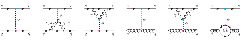
Figure 2: Leading contributions to the semi-leptonic nucleon-electron operators. The combination of light-blue and purple blobs refer to CP-violating effective interaction vertices. Figure from Ref. ⁹⁷.

The effective Lagrangian $\mathcal{L}_{\phi}$ defined in Eq. (3.1) at the scale $\Lambda$ is renormalized at lower energies by QED and QCD interactions. In the leading logarithmic approximation, the solution of the renormalization-group equations for the leptonic (pseudo)scalar couplings $y^{\ell\ell}_{S,P}$ gives ⁹⁷

$$y^{\ell\ell}_{S} \simeq y^{\ell\ell}_{S}(\Lambda)+\frac{6\alpha}{\pi}\frac{m_{\ell}}{v}e^{2}C_{\gamma}\log\frac{\Lambda}{\mu}~{},$$ (33)

$$y^{\ell\ell}_{P} \simeq y^{\ell\ell}_{P}(\Lambda)-\frac{6\alpha}{\pi}\frac{m_{\ell}}{v}e^{2}{\tilde{C}}_{\gamma}\log\frac{\Lambda}{\mu}~{},$$ (34)

where $\mu$ is the renormalization scale. Instead, in the quark sector, we obtain ⁹⁷

$$\!\!y^{qq}_{S}\simeq ~{}~{}y^{qq}_{S}(\Lambda)\!+\!\frac{m_{q}}{v}\!\left(\frac{6\alpha}{\pi}Q^{2}_{q}e^{2}C_{\gamma}\!+\!\frac{8\alpha_{s}}{\pi}g_{s}^{2}C_{g}\right)\!\log\frac{\Lambda}{\mu}~{},$$ (35)

$$\!y^{qq}_{P}\simeq ~{}~{}y^{qq}_{P}(\Lambda)\!-\!\frac{m_{q}}{v}\!\left(\frac{6\alpha}{\pi}Q^{2}_{q}e^{2}{\tilde{C}}_{\gamma}\!+\!\frac{8\alpha_{s}}{\pi}g_{s}^{2}{\tilde{C}}_{g}\right)\!\log\frac{\Lambda}{\mu}~{}.$$ (36)

Since in Eq. (3.1) we factored out the gauge couplings $e^{2}$ and $g^{2}_{s}$, the coefficients $C_{\gamma,g}$ and $\tilde{C}_{\gamma,g}$ are scale-invariant at one-loop order. Top and bottom contributions are taken into account by the QCD trace anomaly in the gluon-gluon-ALP vertex after they have been integrated out (see Fig. 2), yielding

$$g_{s}^{2}C_{g} \simeq g_{s}^{2}C_{g}(\Lambda)+\frac{\alpha_{s}}{12\pi}\sum_{q=t,b}\frac{vy^{qq}_{S}}{m_{q}}~{},$$ (37)

$$g_{s}^{2}\tilde{C}_{g} \simeq g_{s}^{2}\tilde{C}_{g}(\Lambda)-\frac{\alpha_{s}}{8\pi}\sum_{q=t,b}\frac{vy^{qq}_{P}}{m_{q}}~{},$$ (38)

valid in the limit $m_{q}\gg m_{\phi}$, in agreement with Higgs low-energy theorems ¹⁰¹.

Among the most stringent constraints on the CP-violating ALP interactions stemming from Eq. (3.1), EDMs emerge as the most powerful probes. From the experimental side, there is an outstanding program to improve the current limits on permanent EDMs of molecules, atoms, nuclei and nucleons by several orders of magnitude (see e.g. ¹⁰²). It is therefore mandatory to provide a general framework to systematically account for CP-violating ALP contributions to EDMs, which was missing until recently (see however ^{103, 104, 105}).

The leading low-energy CP-violating Lagrangian relevant for EDMs of molecules, atoms, nuclei and nucleons reads ¹⁰⁶

$$\mathcal{L}_{\rm CPV} =\sum_{i,j=u,d,e}\!\!\!C_{ij}(\overline{f}_{i}f_{i})(\overline{f}_{j}i\gamma_{5}f_{j})+\alpha_{s}C_{Ge}\,GG\,\overline{e}i\gamma_{5}e+\alpha_{s}C_{\tilde{G}e}\,G\tilde{G}\,\overline{e}e$$ (39)

$$-\frac{i}{2}\!\sum_{i=u,d,e}d_{i}\overline{f}_{i}(F\!\cdot\!\sigma)\gamma_{5}f_{i}-\frac{i}{2}\!\sum_{i=u,d}g_{s}d^{C}_{i}\overline{f}_{i}(G\!\cdot\!\sigma)\gamma_{5}f_{i}+\frac{d_{G}}{3}f^{abc}G^{a}\tilde{G}^{b}G^{c}~{},$$

where we omitted color-octet 4-quark operators (as they emerge only at one-loop level in the ALP framework) and the dim-4 $G\tilde{G}$ operator. The latter is assumed to be absent thanks to a UV mechanism addressing the strong CP problem.

Within our EFT approach, $C_{ij}$, $C_{Ge}$ and $C_{\tilde{G}e}$ are generated by the Feynman diagrams of Fig. 2 and read

$$C_{ij}\simeq\frac{v^{2}}{\Lambda^{2}}\frac{y^{ii}_{S}y^{jj}_{P}}{m^{2}_{\phi}}~{},\qquad C_{Ge}=\frac{4\pi}{m^{2}_{\phi}}\frac{v}{\Lambda^{2}}C_{g}y^{ee}_{P}~{},\qquad C_{\tilde{G}e}=\frac{4\pi}{m^{2}_{\phi}}\frac{v}{\Lambda^{2}}\tilde{C}_{g}y^{ee}_{S}~{}.$$ (40)

The last term of Eq. (39) represents the Weinberg operator which is generated by the representative diagrams shown in Fig. 3. The related Wilson coefficient $d_{G}$ reads ⁹⁷

$$d_{G} \simeq\frac{g_{s}\alpha_{s}}{(4\pi)^{3}}\sum_{i=t,b}\!\frac{v^{2}}{\Lambda^{2}}\frac{y^{ii}_{S}y^{ii}_{P}}{4m^{2}_{i}}+\frac{3g_{s}}{\pi^{2}}\frac{g_{s}^{4}C_{g}\tilde{C}_{g}}{\Lambda^{2}}\log\frac{\Lambda}{m_{\phi}}~{},$$ (41)

where the first term refers to the two-loop diagram and holds for $m_{q}\gg m_{\phi}$. Instead, the second term of Eq. (41) arises from the one-loop diagrams of Fig. 3.

Figure 3: Leading contributions to the Weinberg operator. Figure from Ref. ⁹⁷.

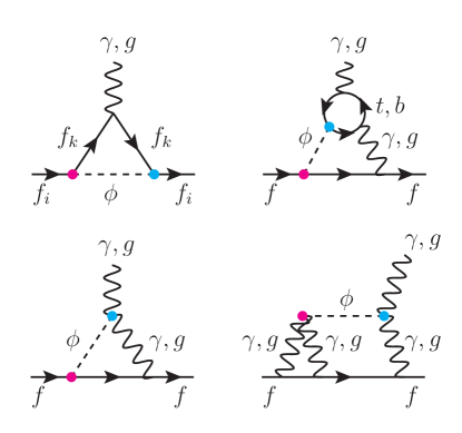
Figure 4: Leading contributions to the fermionic (C)EDMs. Figure from Ref. ⁹⁷.

Finally, we analyse the fermionic (C)EDMs induced by ALP interactions. The leading contributions stem from the Feynman diagrams reported in Fig. 4 and read ^{103, 97}

$$\frac{d_{i}}{e}\simeq -\sum_{k}\frac{Q_{k}}{16\pi^{2}}\frac{m_{k}}{m^{2}_{\phi}}\frac{v^{2}}{\Lambda^{2}}\mbox{Re}\,(y^{ik}_{S}y^{ki}_{P})\,\ell(x_{k})$$

$$-\sum_{k}\frac{N_{c}\,\alpha\,Q_{i}\,Q^{2}_{k}}{8\pi^{3}\,m_{k}}\frac{v^{2}}{\Lambda^{2}}\left(y^{ii}_{P}y^{kk}_{S}f(x_{k})+y^{ii}_{S}y^{kk}_{P}g(x_{k})\right)$$

$$-\frac{Q_{i}}{2\pi^{2}}\frac{v}{\Lambda^{2}}e^{2}(y^{ii}_{S}{\tilde{C}}_{\gamma}-C_{\gamma}y^{ii}_{P})\log\frac{\Lambda}{m_{\phi}}$$

$$-\frac{3\,\alpha\,Q^{3}_{i}}{\pi^{3}}\frac{m_{i}}{\Lambda^{2}}e^{4}C_{\gamma}{\tilde{C}}_{\gamma}\log^{2}\frac{\Lambda}{m_{\phi}}$$

$$-\delta_{qi}\frac{2\,\alpha_{s}\,Q_{i}}{\pi^{3}}\frac{m_{i}}{\Lambda^{2}}e^{2}g^{2}_{s}(C_{\gamma}{\tilde{C}}_{g}+C_{g}{\tilde{C}}_{\gamma})\log^{2}\frac{\Lambda}{m_{\phi}}\,,$$ (42)

in the EDMs case (where $i=e,u,d$, $q=u,d$, and $N_{c}=3$) and

$$d^{C}_{i}\simeq -\sum_{k}\frac{1}{16\pi^{2}}\frac{m_{k}}{m^{2}_{\phi}}\frac{v^{2}}{\Lambda^{2}}\mbox{Re}\,(y^{ik}_{S}y^{ki}_{P})\,\ell(x_{k})$$

$$-\sum_{k}\frac{\alpha_{s}}{16\pi^{3}\,m_{k}}\frac{v^{2}}{\Lambda^{2}}\left(y^{ii}_{P}y^{kk}_{S}f(x_{k})+y^{ii}_{S}y^{kk}_{P}g(x_{k})\right)$$

$$-\frac{1}{2\pi^{2}}\frac{v}{\Lambda^{2}}g_{s}^{2}(y^{ii}_{S}{\tilde{C}}_{g}-C_{g}y^{ii}_{P})\log\frac{\Lambda}{m_{\phi}}$$

$$-\frac{4\,\alpha_{s}}{\pi^{3}}\frac{m_{i}}{\Lambda^{2}}g_{s}^{4}C_{g}{\tilde{C}}_{g}\log^{2}\frac{\Lambda}{m_{\phi}}$$

$$-\frac{3\,\alpha\,Q^{2}_{i}}{2\pi^{3}}\frac{m_{i}}{\Lambda^{2}}e^{2}g_{s}^{2}(C_{\gamma}{\tilde{C}}_{g}+C_{g}{\tilde{C}}_{\gamma})\log^{2}\frac{\Lambda}{m_{\phi}}\,,$$ (43)

for the CEDMs (where $i=u,d$). The loop functions are $\ell(x)=(3\!-\!4x\!+\!x^{2}\!+\!2\log x)/(1-x)^{3}$ where $x_{k}=m^{2}_{k}/m^{2}_{\phi}$ and, in the limit $x\gg 1$, $f(x)\approx(6\log x+13)/18$ and $g(x)\approx(\log x+2)/2$. The first diagram of Fig. 4 accounts for flavour-violating effects (for flavour-diagonal effects, see ¹⁰⁷) while the second diagram refers to Barr-Zee two-loop contributions.

The above expressions have been obtained employing a hard cutoff as a UV regulator and assuming no significant cancellations with finite terms. Although Eqs. (33)-(3.1.1) include only leading-order short-distance effects, the bounds of Table 1 have been derived accounting also for one-loop QCD running effects (improved with a two-loop running of $\alpha_{s}$ and quark masses) from $\Lambda=1$ TeV to $m_{\phi}=5\,$GeV and the running of $\mathcal{L}_{\rm CPV}$ from $m_{\phi}$ to the hadronic scale $\mu_{\rm had}=1$ GeV ¹⁰⁸.

Constraints on $d_{e}$, $C_{ij}$ and $C_{Ge}$ in Eq. (39), are obtained by using the polar molecule ThO. Indeed, the electron spin-precession frequency $\omega_{\text{ThO}}$ is affected by both $d_{e}$ and CP-odd electron–nucleon ($N$) interactions ¹⁰⁹

$$\omega_{\text{ThO}}=1.2\,\mathrm{mrad}/\mathrm{s}\left(\frac{d_{e}}{10^{-29}\,e\,\mathrm{cm}}\right)+1.8\,\mathrm{mrad}/\mathrm{s}\left(\frac{C_{S}}{10^{-9}}\right)~{},$$

where the theoretical error is within a few percent while the experimental limit $\omega_{\text{ThO}}<1.3\,\mathrm{mrad}/\mathrm{s}$ ($90\%$ C.L.) ¹¹⁰. The coefficient $C_{S}$ stemming from the interaction $\mathcal{L}\supset-\frac{G_{F}}{\sqrt{2}}C_{S}\overline{N}N\overline{e}i\gamma_{5}e$ ¹⁰⁹ is related to $C_{ij}$ and $C_{Ge}$ as $C_{S}/v^{2}\simeq-17(C_{ue}+C_{de})+4.7\,\text{GeV}\,C_{Ge}$. The neutron EDM receives contributions from quark (C)EDMs, the Weinberg operator and 4-quark operators ^{111, 112, 82}

$$d_{n} =0.784(28)\,d_{u}-0.204(11)\,d_{d}-0.55(28)\,e\,d^{C}_{u}-1.10(55)\,e\,d^{C}_{d}$$

$$+50(40)\,{\rm MeV}\,e\,d_{G}+30(20)\,{\rm MeV}\,e\,(C_{ud}-C_{du})~{},$$ (44)

and the current experimental bound is $d_{n}<1.8\cdot 10^{-26}\,e~{}$cm ($90\%$ C.L.) ^{50, 51}. Finally, the EDM of the diamagnetic atom ¹⁹⁹Hg is generated by both nuclear and leptonic CP-odd interactions ^{109, 112}

$$d_{\rm Hg}\simeq 4.0\cdot 10^{-4}d_{n}-[2.8\,C_{S}-2.1\,C_{P}]\,10^{-22}\,e\,{\rm cm}~{},$$ (45)

with $C_{P}\simeq C^{(0)}_{P}-C^{(1)}_{P}$ defined through the Lagrangian $\mathcal{L}\supset-\frac{G_{F}}{\sqrt{2}}\overline{N}(C^{(0)}_{P}+\tau_{3}C^{(1)}_{P})i\gamma_{5}N\overline{e}e$. Our bounds are set by employing $C_{P}/v^{2}=350(C_{eu}+C_{ed})+1.1\,\text{GeV}\,C_{\tilde{G}e}$ and the experimental limit $d_{\rm Hg}<6\cdot 10^{-30}e~{}$cm ($90\%$ C.L.) ¹¹³.

CP-violating invariant	Bound	Observable
$|C_{\gamma}{\tilde{C}}_{\gamma}|$	$6.2\times 10^{-3}$	$\omega_{\rm ThO}(d_{e})$
$|C_{g}{\tilde{C}}_{g}|$	$1.4\times 10^{-6}$	$d_{n}(d_{G})$
$|C_{\gamma}{\tilde{C}}_{g}|$	$0.40$	$d_{\rm Hg}(C_{P},C_{S})$
$|C_{g}\tilde{C}_{\gamma}|$	$2.3\times 10^{-3}$	$\omega_{\rm ThO}(C_{S})$
$|y^{ee}_{S}{\tilde{C}}_{\gamma}-y^{ee}_{P}C_{\gamma}|$	$6.9\times 10^{-11}$	$\omega_{\rm ThO}(d_{e})$
$|y^{uu}_{S}{\tilde{C}}_{g}-y^{uu}_{P}C_{g}|$	$8.1\times 10^{-9}$	$d_{n}(d^{C}_{u})$
$|y^{dd}_{S}{\tilde{C}}_{g}-y^{dd}_{P}C_{g}|$	$6.5\times 10^{-9}$	$d_{n}(d^{C}_{d})$
$|y^{ee}_{P}C_{g}|$	$2.1\times 10^{-11}$	$\omega_{\rm ThO}(C_{S})$
$|y^{ee}_{S}\tilde{C}_{g}|$	$7.3\times 10^{-9}$	$d_{\rm Hg}(C_{P})$
$|y^{uu}_{S}y^{dd}_{P}-y^{dd}_{S}y^{uu}_{P}|$	$5.6\times 10^{-9}$	$d_{\rm Hg}(C_{ud}-C_{du})$
$|y^{ee}_{S}y^{uu}_{P}|$, $|y^{ee}_{S}y^{dd}_{P}|$	$4.2\times 10^{-13}$	$d_{\rm Hg}(C_{P})$
$|y^{uu}_{S}y^{ee}_{P}|$, $|y^{dd}_{S}y^{ee}_{P}|$	$2.1\times 10^{-13}$	$\omega_{\rm ThO}(C_{S})$
$|y^{tt}_{S}y^{ee}_{P}|$	$6.8\times 10^{-9}$	$\omega_{\rm ThO}(C_{S})$
$|y^{bb}_{S}y^{ee}_{P}|$	$1.7\times 10^{-10}$	$\omega_{\rm ThO}(C_{S})$
$|y^{ee}_{S}y^{tt}_{P}|$	$8.8\times 10^{-9}$	$\omega_{\rm ThO}(d_{e})$
$|y^{ee}_{S}y^{bb}_{P}|$	$3.9\times 10^{-9}$	$d_{\rm Hg}(C_{P})$
$|y^{tt}_{S}y^{tt}_{P}|$	$0.10$	$d_{n}(d_{G})$
$|y^{bb}_{S}y^{bb}_{P}|$	$5.9\times 10^{-5}$	$d_{n}(d_{G})$
$|y^{ee}_{S}\,y^{ee}_{P}|$	$1.0\times 10^{-10}$	$\omega_{\rm ThO}(d_{e})$
$|y^{e\mu}_{S}\,y^{\mu e}_{P}|$	$2.2\times 10^{-12}$	$\omega_{\rm ThO}(d_{e})$
$|y^{e\tau}_{S}\,y^{\tau e}_{P}|$	$3.1\times 10^{-12}$	$\omega_{\rm ThO}(d_{e})$
$|y^{uu}_{S}\,y^{uu}_{P}|$	$3.9\times 10^{-8}$	$d_{n}(d^{C}_{u})$
$|y^{uc}_{S}\,y^{cu}_{P}|$	$3.2\times 10^{-9}$	$d_{n}(d^{C}_{u})$
$|y^{ut}_{S}\,y^{tu}_{P}|$	$3.2\times 10^{-7}$	$d_{n}(d^{C}_{u})$
$|y^{dd}_{S}\,y^{dd}_{P}|$	$4.6\times 10^{-8}$	$d_{n}(d^{C}_{d})$
$|y^{ds}_{S}\,y^{sd}_{P}|$	$6.4\times 10^{-9}$	$d_{n}(d^{C}_{d})$
$|y^{db}_{S}\,y^{bd}_{P}|$	$1.7\times 10^{-8}$	$d_{n}(d^{C}_{d})$

Table 1: Bounds on CP-violating invariants for $\Lambda=1$ TeV and $m_{\phi}=5$ GeV. In the 3rd column we specify the observable and the leading operator setting the bound (in brackets).

The EDM’s sensitivity to the CP-violating invariants defined in Eq. (32) are reported in Table 1 for $m_{\phi}=5$ GeV. As we can see, 4-fermion operators set the strongest bounds on several CP invariants. Moreover, the Weinberg operator is particularly effective in constraining ALP couplings to top and bottom quarks as well as to gluons. Interestingly, EDMs put severe bounds also to flavor-violating sources of CP violation that are competitive with those stemming from flavour-changing neutral current processes. Even if the relative impact of the above contributions on the EDMs will depend on the specific ALP model, it is instructive to consider a realistic example where $y^{ii}_{S,P}\propto\frac{m_{i}}{v}$, $C_{\gamma(g)}$ and $\tilde{C}_{\gamma(g)}\propto\frac{1}{16\pi^{2}}$. In this case, 4-fermion operators are the best probes of CP violation followed by the electron EDM and the Weinberg operator which show similar sensitivities. Let us also remark that the electron EDM bounds are always stronger than the limits from the anomalous magnetic moment of the electron, unless CP-violating phases are smaller than about $10^{-4}$ ¹¹⁴. Future experimental projections are particularly promising. The experimental bound on the neutron EDM measurement should reach the level of $d_{n}\lesssim 10^{-28}e~{}$cm ¹⁰². There are also plans to measure the proton and deuteron EDMs in electromagnetic storage rings at the level of $d_{p,D}\lesssim 10^{-29}e~{}$cm ¹⁰². Furthermore, we expect also one order of magnitude improvement on the current measurement of molecular systems, e.g. the polar molecule ThO, which currently sets the most powerful bounds on the electron EDM and electron-nucleon couplings. If the above forecasts are respected, the limits on $d_{G}$ and quark (C)EDMs will improve by roughly three orders of magnitude while the constraints on electron EDM and 4-fermion contributions will be strengthened by one order of magnitude.

3.2 CP-violating ALP Lagrangian: $m_{\phi}\lesssim 1$ GeV

In this section, we are going to extend the previous analysis to ALP masses in the sub-GeV region, where non-perturbative methods, such as chiral perturbation theory ($\chi$pt), have to be employed. The construction of the effective chiral Lagrangian for an ALP interacting with photons and light pseudoscalar mesons has been already discussed at length in the literature for the case of a CP-odd ALP (see Refs. ^{29, 115, 116, 117}, as well as ^{118, 119, 120, 121, 122} for analyses beyond leading order in $\chi\text{pt}$). The development of the chiral Lagrangian for CP-even scalar interactions was elaborated instead in Ref. ¹²³. While we refer to Ref. ⁹⁸ for the construction of the most general chiral Lagrangian at $\mathcal{O}(p^{2})$ describing CP-violating interactions of a light ALP with mesons and baryons, we report here the main results needed to estimate the ALP contribution to the EDMs.

To match the notation of Ref. ⁹⁸ we start from a slightly different version of the ALP effective Lagrangian, compared to the one in Eq. (3.1), featuring a derivative ALP coupling to the quark axial current, namely

$$\mathcal{L}_{\phi}^{\text{QCD}} =e^{2}\frac{\tilde{C}_{\gamma}}{\Lambda}\phi F\tilde{F}+g_{s}^{2}\frac{\tilde{C}_{g}}{\Lambda}\phi G\tilde{G}+\frac{\partial_{\mu}\phi}{\Lambda}\overline{q}\,\gamma^{\mu}Y_{P}\gamma_{5}\,q$$

$$+e^{2}\frac{C_{\gamma}}{\Lambda}\phi FF+g_{s}^{2}\frac{C_{g}}{\Lambda}\phi GG+\frac{v}{\Lambda}\,\phi\,\overline{q}\,y_{S}\,q~{},$$ (46)

that is valid above the GeV scale. Here, $q^{T}=(u,d)$, while $Y_{P}$ and $y_{S}$ are hermitian matrices.

Upon taking into account hadronization effects, following a chiral representation of the ALP interactions with quarks and gluons, Ref. ⁹⁸ obtained a low-energy effective Lagrangian describing the interaction of the ALP with light particles: photons, leptons, pions and nucleons. The ALP effective Lagrangian can be cast in two contributions displaying opposite CP transformation properties, given respectively by (in the case of two active flavours, $N_{f}=2$) ⁹⁸

$$\mathcal{L}_{\phi,\text{\,CP-even}}^{\chi\text{pt}} =e^{2}\frac{c_{\gamma}}{\Lambda}\,\phi\,FF+\frac{v}{\Lambda}y_{\ell,S}^{ij}\,\phi\,\overline{\ell}_{i}\ell_{j}+\kappa\,\frac{\phi}{\Lambda}\,\left[\partial^{\mu}\pi_{0}\partial_{\mu}\pi_{0}+2\partial^{\mu}\pi^{+}\partial_{\mu}\pi^{-}\right]$$

$$+\frac{\phi}{\Lambda}\,(\pi_{0}^{2}+2\pi^{+}\pi^{-})m_{\pi}^{2}\left[\frac{v}{2}\frac{\mathcal{Z}_{u}+\mathcal{Z}_{d}}{m_{u}+m_{d}}-2\,\kappa\right]+\frac{\phi}{\Lambda}C_{\phi\text{NN}}\overline{N}N$$ (47)

and

$$\mathcal{L}_{\phi,\text{\,CP-odd}}^{\chi\text{pt}} =e^{2}\frac{\tilde{c}_{\gamma}}{\Lambda}\,\phi\,F\tilde{F}+i\frac{v}{\Lambda}y_{\ell,P}^{ij}\,\phi\,\overline{\ell}_{i}\gamma_{5}\ell_{j}+\frac{\phi}{\Lambda}\,\pi_{0}(\pi_{0}^{2}+2\pi^{+}\pi^{-})\left[\frac{m_{\pi}^{2}m_{\phi}^{2}}{m_{\pi}^{2}-m_{\phi}^{2}}\frac{\Delta^{A}_{ud}}{6f_{\pi}\Lambda}\right]$$

$$+\frac{2}{3}\frac{\Delta^{A}_{ud}}{f_{\pi}\Lambda}\frac{m_{\pi}^{2}}{m_{\pi}^{2}-m_{\phi}^{2}}\,\partial^{\mu}\phi\,(\pi_{0}\pi^{-}\partial_{\mu}\pi^{+}+\pi_{0}\pi^{+}\partial_{\mu}\pi^{-}-2\pi^{+}\pi^{-}\partial_{\mu}\pi^{0})$$

$$+\frac{\partial_{\mu}\phi}{\Lambda}\overline{N}\tilde{C}_{\phi\text{N}}\gamma^{\mu}\gamma_{5}N~{},$$ (48)

where explicit expressions for the parameters appearing in the above Lagrangians in terms of the short-distance parameters of Eq. (3.2) are reported below in Eq. (3.2). In particular, the physical ALP mass after diagonalization of the ALP-pion system reads ⁹⁸

$$m^{2}_{\phi}=M_{\phi}^{2}+m_{\pi}^{2}(\lambda_{g})^{2}\frac{m_{u}m_{d}}{(m_{u}+m_{d})^{2}}\frac{f_{\pi}^{2}}{\Lambda^{2}}+m_{\pi}^{2}\frac{M_{\phi}^{4}}{(m_{\pi}^{2}-M_{\phi}^{2})^{2}}(\Delta^{A}_{ud})^{2}\frac{f_{\pi}^{2}}{\Lambda^{2}}~{},$$ (49)

where $M_{\phi}$ is the bare ALP mass and $\lambda_{g}=32\pi^{2}\tilde{C}_{g}$.

	$c_{\gamma}$	$y_{\ell,S}$	$\kappa$	$\mathcal{Z}$	$C_{\phi\text{NN}}$
$\tilde{c}_{\gamma}$	$\tilde{c}_{\gamma}\,c_{\gamma}$	$\tilde{c}_{\gamma}\,y_{\ell,S}$	$\tilde{c}_{\gamma}\,\kappa$	$\tilde{c}_{\gamma}\,\mathcal{Z}$	$\tilde{c}_{\gamma}\,C_{\phi\text{NN}}$
$y_{\ell,P}$	$y_{\ell,P}\,c_{\gamma}$	$y_{\ell,P}\,y_{\ell,S}$	$y_{\ell,P}\,\kappa$	$y_{\ell,P}\,\mathcal{Z}$	$y_{\ell,P}\,C_{\phi\text{NN}}$
$\Delta_{ud}^{A}$	$\Delta_{ud}^{A}\,c_{\gamma}$	$\Delta_{ud}^{A}\,y_{\ell,S}$	$\Delta_{ud}^{A}\,\kappa$	$\Delta_{ud}^{A}\,\mathcal{Z}$	$\Delta_{ud}^{A}\,C_{\phi\text{NN}}$
$\tilde{C}_{\phi\text{N}}$	$\tilde{C}_{\phi\text{N}}\,c_{\gamma}$	$\tilde{C}_{\phi\text{N}}\,y_{\ell,S}$	$\tilde{C}_{\phi\text{N}}\,\kappa$	$\tilde{C}_{\phi\text{N}}\,\mathcal{Z}$	$\tilde{C}_{\phi\text{N}}\,C_{\phi\text{NN}}$

Table 2: Jarlskog invariants emerging from the interactions in Eq. (3.2) and (3.2).

Note that, independently of the scalar or pseudo-scalar nature of the ALP field, CP violation is unavoidable as long as at least one CP-even and one CP-odd couplings from Eq. (3.2) and (3.2) are simultaneously non-vanishing. CP-violating effects can be described in terms of low-energy Jarlsokg invariants, which are reported in Table 2. In particular, the coefficients appearing in Table 2 are related to the microscopic parameters of Eq. (3.2) via the following relations ⁹⁸

$$c_{\gamma} =C_{\gamma}-\frac{\beta^{0}_{\text{QED}}}{\beta^{0}_{\text{QCD}}}C_{g}~{},\qquad\tilde{c}_{\gamma}=\,\tilde{C}_{\gamma}-4N_{c}\text{ tr }(Q_{A}Q_{q}^{2})\tilde{C}_{g}~{},\qquad\kappa=\frac{8\pi}{\alpha_{s}}\frac{g_{s}^{2}C_{g}}{\beta^{0}_{\text{QCD}}}~{},$$

$$\mathcal{Z} =y_{S}+\frac{g_{s}^{2}C_{g}}{\beta^{0}_{\text{QCD}}}\frac{8\pi}{\alpha_{s}}\frac{M_{q}}{v}~{},\qquad\Delta^{A}_{ud}=Y_{P}^{u}-Y_{P}^{d}-16\pi^{2}\tilde{C}_{g}\frac{m_{d}-m_{u}}{m_{d}+m_{u}}~{},$$

$$\tilde{C}_{\phi\text{p}} =Y_{P}^{u}\Delta_{u}+Y_{P}^{d}\Delta_{d}-16\pi^{2}\tilde{C}_{g}\left[\frac{m_{u}\Delta_{d}}{m_{u}+m_{d}}+\frac{m_{d}\Delta_{u}}{m_{u}+m_{d}}-\frac{m_{\phi}^{2}\Delta^{A}_{ud}}{m_{\pi}^{2}-m_{\phi}^{2}}\frac{\Delta_{u}-\Delta_{d}}{32\pi^{2}\tilde{C}_{g}}\right]~{},$$

$$\tilde{C}_{\phi\text{n}} =Y_{P}^{u}\Delta_{d}-Y_{P}^{d}\Delta_{u}-16\pi^{2}\tilde{C}_{g}\left[\frac{m_{u}\Delta_{u}}{m_{u}+m_{d}}+\frac{m_{d}\Delta_{d}}{m_{u}+m_{d}}+\frac{m_{\phi}^{2}\Delta^{A}_{ud}}{m_{\pi}^{2}-m_{\phi}^{2}}\frac{\Delta_{u}-\Delta_{d}}{32\pi^{2}\tilde{C}_{g}}\right]~{},$$

$$C_{\phi\text{pp}} =\frac{y_{q,S}^{u}\,v}{m_{u}}\,\sigma_{u}+\frac{y_{q,S}^{d}\,v}{m_{d}}\,\sigma_{d}+\frac{y_{q,S}^{s}\,v}{m_{s}}\,\sigma_{s}-\frac{32\pi^{2}C_{g}}{9}\,(m_{p}-\sigma_{u}-\sigma_{d}-\sigma_{s})~{},$$

$$C_{\phi\text{nn}} =\frac{y_{q,S}^{u}\,v}{m_{d}}\,\sigma_{d}+\frac{y_{q,S}^{d}\,v}{m_{u}}\,\sigma_{u}+\frac{y_{q,S}^{s}\,v}{m_{s}}\,\sigma_{s}-\frac{32\pi^{2}C_{g}}{9}\,(m_{p}-\sigma_{u}-\sigma_{d}-\sigma_{s})~{},$$ (50)

with the low-energy QCD matrix elements given by $\Delta_{u}=0.858(22)$ and $\Delta_{d}=-0.418(22)$ ^{124, 125}, while the values of $\sigma_{u}$, $\sigma_{d}$ and $\sigma_{s}$ can be found e.g. in Ref. ¹²⁶.

3.2.1 ALP contribution to EDMs

The effective Lagrangian provided in Eqs. (3.2)–(3.2) readily allows one to compute the contributions of a light ALP to the proton EDM, with the relevant topologies displayed in Fig. 5. Following the standard definition of the EDM of a fermion given in Eq. (39), one finds ⁹⁸

$$d_{p} \simeq-\frac{e\,Q_{p}}{4\pi^{2}\Lambda^{2}}\left[C_{\phi\text{pp}}\tilde{C}_{\phi\text{p}}+e^{2}m_{p}c_{\gamma}\tilde{C}_{\phi\text{p}}\left(6+2\ln\frac{\Lambda_{\text{ren}}^{2}}{m_{p}^{2}}\right)+e^{2}\tilde{c}_{\gamma}C_{\phi\text{pp}}\left(2+\ln\frac{\Lambda_{\text{ren}}^{2}}{m_{p}^{2}}\right)\right.$$

$$\left.+3\frac{Q_{p}^{2}}{\pi^{2}}m_{p}e^{6}c_{\gamma}\tilde{c}_{\gamma}\ln^{2}\frac{\Lambda_{\text{ren}}}{m_{\phi}}\right]~{},$$ (51)

in the limit $m_{\phi}\ll m_{p}$ and setting the renormalization scale $\Lambda_{\rm ren}\simeq m_{p}$.

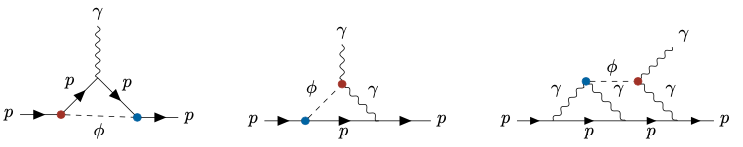
Figure 5: Feynman diagrams contributing to the ALP-mediated effects to the proton EDM, $d_{p}$. Figure from Ref. ⁹⁸.

Due to their lack of a minimal coupling to the electromagnetic field-strength tensor, neutrons cannot develop an EDM at leading order in $\chi$pt. However, they do display non-minimal couplings to photons at next-to-leading order in $\chi$pt ^{127, 128} which can eventually induce a non-zero value for $d_{n}$. In the $N_{f}=2$ case, the relevant relativistic Lagrangian reads

$$\mathcal{L}_{\gamma\text{N}}^{\text{NLO}}=\frac{F_{\mu\nu}}{4m_{N}}\left[\,\mathcal{C}_{p}\,\overline{p}\sigma^{\mu\nu}p+\mathcal{C}_{n}\,\overline{n}\sigma^{\mu\nu}n\,\right]~{},$$ (52)

where $\mathcal{C}_{p}\simeq 1.79$ ¹²⁵ and $\mathcal{C}_{n}\simeq 1.91$ ¹²⁵ are measured low-energy constants. Given these interactions, one can then compute the corresponding contribution to $d_{n}$, whose Feynman diagrams are the same as for the proton case, finding the following order of magnitude estimate ⁹⁸

$$d_{n}\sim-\frac{e\,\mathcal{C}_{n}}{4\pi^{2}\Lambda^{2}}\left[-\frac{3}{8}C_{\phi\text{nn}}\tilde{C}_{\phi\text{n}}\frac{\Lambda_{\text{ren}}^{2}}{m_{n}^{2}}+e^{2}(2m_{n}c_{\gamma}\tilde{C}_{\phi\text{n}}+3\tilde{c}_{\gamma}C_{\phi\text{nn}})\ln\frac{\Lambda_{\text{ren}}^{2}}{m_{n}^{2}}\right]~{}.$$ (53)

Note that $d_{p}$ and $d_{n}$ have a comparable size while their current experimental bounds read $d_{p}<2.1\times 10^{-25}\,e$ cm ¹²⁹ and $d_{n}<1.8\times 10^{-26}\,e$ cm (90% C.L.) ^{50, 51}.

Constraints on the low-energy Jarlskog invariants are obtained by imposing the existing bounds on $d_{p}$ and $d_{n}$. Turning on just two couplings at a time, one finds the limits displayed in Table 3.

	$y_{S}^{u}$	$y_{S}^{d}$	$C_{\gamma}$	$C_{g}$
$y_{P}^{u}$	$2.8\times 10^{-12}$	$1.8\times 10^{-12}$	$8.0\times 10^{-8}$	$1.1\times 10^{-10}$
$y_{P}^{d}$	$9.9\times 10^{-12}$	$6.4\times 10^{-12}$	$1.1\times 10^{-7}$	$3.8\times 10^{-10}$
$\tilde{C}_{\gamma}$	$1.2\times 10^{-6}$	$1.8\times 10^{-6}$	$4.8\times 10^{-3}$	$7.1\times 10^{-5}$
$\tilde{C}_{g}$	$1.1\times 10^{-9}$	$7.4\times 10^{-10}$	$2.4\times 10^{-5}$	$4.4\times 10^{-8}$

Table 3: Upper limits on Jarlskog invariants obtained from the bounds on the neutron and proton EDMs assuming $\Lambda=1$ TeV ⁹⁸. To make contact with the notation in Eq. (3.1) here we have defined $y_{P}^{q}=-2\frac{m_{q}}{v}Y_{P}^{q}$.

3.3 Towards a UV completion for the CP-violating ALP

It is interesting to speculate on the possible origin of the CP-violating ALP effective Lagrangian in Eq. (3.1). The underlying UV dynamics can be naturally conceived in the framework of strongly-coupled theories. A paradigmatic example is given by the SM itself, when considering the effective interactions of the neutral pion $\pi^{0}$ below the GeV scale (see e.g. ¹³⁰). In this setup, the role of the ALP is played by $\pi^{0}$, quark masses induce the breaking of the shift symmetry while the QCD $\theta$ term provides the necessary CP-violating source. Finally, electromagnetic interactions act as mediators from the strong sector to the $\pi^{0}$. CP-odd pion interactions include the terms

$$A_{1}\frac{\pi^{0}}{f_{\pi}}F\tilde{F}+A_{2}\frac{\partial_{\mu}\pi^{0}}{f_{\pi}}\overline{e}\gamma^{\mu}\gamma_{5}e~{},\\$$ (54)

where $A_{1}=\frac{\alpha}{4\pi}$ is the Wess-Zumino-Witten term and $A_{2}$ is radiatively induced by $A_{1}$ via electromagnetic interactions, so that $A_{2}\sim(\frac{\alpha}{4\pi})^{2}$. CP-even pion interactions

$$C_{1}\frac{\pi^{0}}{f_{\pi}}FF+C_{2}m_{e}\frac{\pi^{0}}{f_{\pi}}\overline{e}e~{},$$ (55)

are instead sourced by the QCD $\theta$ term. In particular, $C_{1}$ emerges from integrating out heavy charged-baryon loops. The CP-even Yukawa-like couplings between pions and baryons appearing in such triangle loops naturally emerge from the baryonic Lagrangian upon including the $\theta$ term in the phase of the quark mass matrix. $C_{2}$ is in turn generated radiatively from $C_{1}$ via electromagnetic interactions and thus scales as $C_{2}\sim\theta\frac{\alpha}{4\pi}$. Strongly coupled new physics scenarios emerging at the scale $\Lambda\gtrsim 1$ TeV, that mimic the pion dynamics of the SM, can hence be conceived in analogy.

Other interesting scenarios motivating the study of a CP-violating ALP are provided by relaxion models ¹³¹, aiming at solving the hierarchy problem through an ALP field, the relaxion, which scans the Higgs boson mass in the early Universe from a very high-energy scale $\mu\gg 1$ TeV down to the final value of $\mathcal{O}(v)$. The presence of both the relaxion-Higgs mixing and the relaxion-photon/gluon couplings does violate CP. As an explicit example let us consider the following relaxion Lagrangian

$$\mathcal{L}_{\text{Relax}} =\frac{1}{2}\partial^{\mu}\Phi\partial_{\mu}\Phi-\frac{\Phi}{\Lambda}\left(\tilde{\mathcal{C}}_{g}\,g_{s}^{2}\,G\tilde{G}+\tilde{\mathcal{C}}_{W}\,g^{2}\,W\tilde{W}+\tilde{\mathcal{C}}_{B}\,g^{\prime 2}\,B\tilde{B}\right)$$

$$+\frac{\partial^{\mu}\Phi}{\Lambda}\sum_{f}\overline{\psi}_{f}\gamma_{\mu}\tilde{X}_{f}\psi_{f}-V(H,\Phi)~{},$$ (56)

where $\Phi$ is the relaxion field and $f=\left\{\ell_{L},q_{L},u_{R},d_{R},e_{R}\right\}$ are the chiral SM fermions, and the relaxion-Higgs potential is given by (see e.g. ^{131, 132, 133, 134})

$$V(H,\Phi) =\left[-\mu^{2}+\tilde{g}\mu\Phi\right]|H^{\dagger}H|-M^{2}|H^{\dagger}H|\cos\left(\frac{\Phi}{\Lambda}\right)$$

$$+\lambda\,|H^{\dagger}H|^{2}+r\tilde{g}\mu^{3}\Phi+(m_{\phi}^{0})^{2}\Phi^{2}+\dots~{}.$$ (57)

Of these terms, the linear one in $\Phi$ prompts the cosmological evolution of the relaxion field, which allows for scanning of the Higgs VEV via the relaxion-dependent Higgs mass parameter. The cosine term acts instead as a backreaction, producing the potential barrier that eventually halts the evolution of the relaxion field around the Higgs VEV. Expanding both the Higgs and relaxion fields around their VEV,

$$\Phi=\phi_{0}+\phi^{\prime}\qquad\text{and}\qquad H=\frac{1}{\sqrt{2}}\begin{pmatrix}0\\ v+h^{\prime}\end{pmatrix}~{},$$ (58)

generates in turn a mixing between the Higgs and the relaxion fields, with the mass eigenstates, $\phi=c_{\theta}\phi^{\prime}+s_{\theta}h^{\prime}$ and $h=c_{\theta}h^{\prime}-s_{\theta}\phi^{\prime}$, given in terms of the mixing angle $s_{\theta}\simeq\frac{1}{2\lambda}\frac{M^{2}}{v^{2}}\frac{v}{\Lambda}\sin\frac{\phi_{0}}{\Lambda}\ll 1$. The resulting interaction Lagrangian in the mass eigenbasis at $\mathcal{O}(1/\Lambda)$ is given by

$$\mathcal{L}_{\text{Relax}} \supset c_{\theta}\frac{\partial_{\mu}\phi}{\Lambda}\sum_{f}\overline{f}\,\gamma^{\mu}(X_{f}^{V}+X_{f}^{A}\gamma_{5})f-s_{\theta}\frac{\phi}{v}\sum_{f}\frac{m_{f}}{v}\overline{f}f$$

$$-c_{\theta}\frac{\phi}{\Lambda}\Bigg{[}\tilde{\mathcal{C}}_{g}\,g_{s}^{2}\,G\tilde{G}+e^{2}\Big{(}\tilde{\mathcal{C}}_{\gamma}F\tilde{F}+2\frac{\tilde{\mathcal{C}}_{\gamma Z}}{s_{w}c_{w}}F\tilde{Z}+\frac{\tilde{\mathcal{C}}_{Z}}{s_{w}^{2}c_{w}^{2}}Z\tilde{Z}\Big{)}$$

$$+\,\tilde{\mathcal{C}}_{W}\,g^{2}\,\left(W^{+\mu\nu}\tilde{W}^{-}_{\mu\nu}-2ig(s_{w}A_{\nu}+c_{w}Z_{\nu})W_{\mu}^{+}\tilde{W}^{-\mu\nu}\right.$$

$$\left.+2igW_{\mu}^{+}W_{\nu}^{-}(c_{w}\tilde{F}^{\mu\nu}+s_{w}\tilde{Z}^{\mu\nu})+\text{h.c.}\right)\Bigg{]}+s_{\theta}\frac{\phi}{v}\left(\frac{2}{3}\mathcal{C}_{g}\,g_{s}^{2}\,GG+2\mathcal{C}_{\gamma}e^{2}FF\right)$$

$$-\left(\varphi^{+}\varphi^{-}+\frac{\varphi_{Z}^{2}}{2}\right)\left[c_{\theta}\frac{\phi}{\Lambda}M^{2}\sin\frac{\phi_{0}}{\Lambda}+2s_{\theta}\lambda\phi v+2c_{\theta}s_{\theta}\phi h\right]$$

$$+2s_{\theta}\frac{\phi}{v}\left(\!m_{W}^{2}W^{+}_{\mu}W^{-\mu}\!+\frac{m_{Z}^{2}}{2}Z_{\mu}Z^{\mu}\right)\!+2s_{\theta}c_{\theta}\frac{\phi h}{v^{2}}\left(\!m_{W}^{2}W_{\mu}^{+}W^{-\mu}\!+\frac{m_{Z}^{2}}{2}Z_{\mu}Z^{\mu}\right)$$

$$-3\lambda c_{\theta}^{2}s_{\theta}h^{2}\phi-\lambda c_{\theta}^{3}s_{\theta}h^{3}\phi-c_{\theta}^{3}\frac{\phi h^{2}}{\Lambda}M^{2}\sin\frac{\phi_{0}}{\Lambda}+\mathcal{L}_{\text{Higgs}}^{\text{kin}}(c_{\theta}h\rightarrow s_{\theta}\phi)~{},$$ (59)

where $\mathcal{L}_{\text{Higgs}}^{\text{kin}}$ is the Lagrangian piece containing all the interactions between the Higgs boson, the electroweak gauge bosons and the respective Goldstones that stem from the Higgs kinetic term. Moreover, we have defined $2X_{V/A}^{f}=(K_{f}^{\dagger}\tilde{X}_{R}^{f}K_{f}\,\pm\,U_{f}^{\dagger}\tilde{X}_{L}^{f}U_{f})$, where $K_{f}$ and $U_{f}$ are the right-handed and left-handed fermion rotation matrices needed to go from the interaction basis to the mass basis.

The Lagrangian in Eq. (3.3) has then to be evolved down to the QCD scale. This procedure includes both integrating out heavy particle states and the running of Wilson coefficients ¹⁰⁰. Finally, the resulting Lagrangian can be matched onto the effective one in Eq. (3.2), yielding

$$C_{\gamma} =2\,s_{\theta}\,\mathcal{C}_{\gamma}\frac{\Lambda}{v}~{},\qquad C_{g}=\frac{2}{3}\,s_{\theta}\,\mathcal{C}_{g}\frac{\Lambda}{v}~{},$$ (60)

$$\tilde{C}_{\gamma} =-2\,c_{\theta}\,\tilde{\mathcal{C}}_{\gamma}~{},\qquad\,\tilde{C}_{g}=-\,c_{\theta}\,\tilde{\mathcal{C}}_{g}~{},$$ (61)

$$y_{s} =-s_{\theta}\,\frac{M_{q}}{v}\frac{\Lambda}{v}~{},\quad\,Y_{P}=c_{\theta}\,\frac{K_{f}^{\dagger}\tilde{X}_{R}^{f}K_{f}-U_{f}^{\dagger}\tilde{X}_{L}^{f}U_{f}}{2}~{}.$$ (62)

4 Conclusions

In this review, we explored the theoretical landscape of CP-violating axions, delving into both the well-established framework of QCD axions and the broader setup of ALPs. Our discussion centred around two main themes: the implications of CP violation for axion-mediated forces in the context of QCD axions and the effective interactions of CP-violating ALPs, emphasizing their contributions to EDMs.

The structural sensitivity of the QCD axion to high-energy sources of CP violation, as shown by the estimate in Eq. (11), suggests rethinking the role of the axion, to be considered not just as a “laundry soap” of CP violation in strong interactions, but rather as a low-energy portal to high-energy sources of CP violation, thus turning the “strong CP problem” into the “strong CP opportunity”. In particular, axion-mediated forces, which are enhanced by the presence of a CP-violating axion coupling to nucleons, provide an extra experimental handle for probing UV sources of CP violation in the quark sector, with projected sensitivities that are stronger (in a given range of axion masses, cf. Fig. 1) than current EDM limits. Moreover, if the origin of CP-violating axion couplings does not stem from QCD-coupled physics, like e.g. in the presence of PQ-breaking operators, the CP-violating axion potential is unsuppressed above the temperatures of the QCD crossover, and the relative enhancement compared to the CP-preserving QCD potential might lead to sizeable deviations in the axion relic abundance from the misalignment mechanism. However, as discussed in Sect. 2.4, the relative enhancement is only sufficient to achieve such deviation in the regime in which the axion provides a sub-fraction of dark matter, unless tuning is invoked to relax the nEDM constraint.

In the second part, we reviewed the contribution of CP-violating ALP interactions to EDMs of nucleons, nuclei, atoms and molecules, following two recent works ^{97, 98}, respectively for the case of ALP masses above and below the GeV scale. In the latter case, we employed a chiral Lagrangian approach to parametrize the general CP-violating interactions of the ALP with pions and nucleons.

The analysis of CP-violating ALPs could be expanded in several directions. For instance, it could be worth to construct explicit UV completions of the CP-violating ALP effective Lagrangian, which were briefly sketched in Sect. 3.3. Another interesting path would be to investigate whether a successful baryogenesis mechanism can be driven by an ALP field ^{135, 136, 137, 138, 139}, thus providing a rationale for exploring CP-violating ALP interactions.

References

• Peccei and Quinn 1977 R. D. Peccei and H. R. Quinn, Phys. Rev. Lett., 1977, 38, 1440–1443.
• Peccei and Quinn 1977 R. D. Peccei and H. R. Quinn, Phys. Rev. D, 1977, 16, 1791–1797.
• Weinberg 1978 S. Weinberg, Phys. Rev. Lett., 1978, 40, 223–226.
• Wilczek 1978 F. Wilczek, Phys. Rev. Lett., 1978, 40, 279–282.
• Preskill et al. 1983 J. Preskill, M. B. Wise and F. Wilczek, Phys. Lett., 1983, 120B, 127–132.
• Abbott and Sikivie 1983 L. F. Abbott and P. Sikivie, Phys. Lett., 1983, 120B, 133–136.
• Dine and Fischler 1983 M. Dine and W. Fischler, Phys. Lett., 1983, 120B, 137–141.
• Irastorza and Redondo 2018 I. G. Irastorza and J. Redondo, Prog. Part. Nucl. Phys., 2018, 102, 89–159.
• Sikivie 2021 P. Sikivie, Rev. Mod. Phys., 2021, 93, 015004.
• Graham and Rajendran 2013 P. W. Graham and S. Rajendran, Phys. Rev. D, 2013, 88, 035023.
• Budker et al. 2014 D. Budker, P. W. Graham, M. Ledbetter, S. Rajendran and A. Sushkov, Phys. Rev. X, 2014, 4, 021030.
• Arvanitaki and Geraci 2014 A. Arvanitaki and A. A. Geraci, Phys. Rev. Lett., 2014, 113, 161801.
• Geraci et al. 2018 A. A. Geraci et al., Springer Proc. Phys., 2018, 211, 151–161.
• Di Luzio et al. 2022 L. Di Luzio et al., Eur. Phys. J. C, 2022, 82, 120.
• Barbieri et al. 2017 R. Barbieri, C. Braggio, G. Carugno, C. S. Gallo, A. Lombardi, A. Ortolan, R. Pengo, G. Ruoso and C. C. Speake, Phys. Dark Univ., 2017, 15, 135–141.
• Crescini et al. 2017 N. Crescini, C. Braggio, G. Carugno, P. Falferi, A. Ortolan and G. Ruoso, Nucl. Instrum. Meth., 2017, A842, 109–113.
• Crescini et al. 2017 N. Crescini, C. Braggio, G. Carugno, P. Falferi, A. Ortolan and G. Ruoso, Phys. Lett., 2017, B773, 677–680.
• Crescini et al. 2020 N. Crescini et al., Phys. Rev. Lett., 2020, 124, 171801.
• Kim 1979 J. E. Kim, Phys. Rev. Lett., 1979, 43, 103.
• Shifman et al. 1980 M. A. Shifman, A. I. Vainshtein and V. I. Zakharov, Nucl. Phys., 1980, B166, 493.
• Zhitnitsky 1980 A. R. Zhitnitsky, Sov. J. Nucl. Phys., 1980, 31, 260.
• Dine et al. 1981 M. Dine, W. Fischler and M. Srednicki, Phys. Lett., 1981, B104, 199–202.
• Davidson and Wali 1982 A. Davidson and K. C. Wali, Phys. Rev. Lett., 1982, 48, 11.
• Wilczek 1982 F. Wilczek, Phys. Rev. Lett., 1982, 49, 1549–1552.
• Berezhiani 1983 Z. G. Berezhiani, Phys. Lett. B, 1983, 129, 99–102.
• Ema et al. 2017 Y. Ema, K. Hamaguchi, T. Moroi and K. Nakayama, JHEP, 2017, 01, 096.
• Calibbi et al. 2017 L. Calibbi, F. Goertz, D. Redigolo, R. Ziegler and J. Zupan, Phys. Rev. D, 2017, 95, 095009.
• Björkeroth et al. 2019 F. Björkeroth, L. Di Luzio, F. Mescia and E. Nardi, JHEP, 2019, 02, 133.
• Georgi et al. 1986 H. Georgi, D. B. Kaplan and L. Randall, Phys. Lett. B, 1986, 169, 73–78.
• Mimasu and Sanz 2015 K. Mimasu and V. Sanz, JHEP, 2015, 06, 173.
• Jaeckel and Spannowsky 2016 J. Jaeckel and M. Spannowsky, Phys. Lett. B, 2016, 753, 482–487.
• Knapen et al. 2017 S. Knapen, T. Lin, H. K. Lou and T. Melia, Phys. Rev. Lett., 2017, 118, 171801.
• Brivio et al. 2017 I. Brivio, M. B. Gavela, L. Merlo, K. Mimasu, J. M. No, R. del Rey and V. Sanz, Eur. Phys. J. C, 2017, 77, 572.
• Bauer et al. 2017 M. Bauer, M. Neubert and A. Thamm, Phys. Rev. Lett., 2017, 119, 031802.
• Bauer et al. 2017 M. Bauer, M. Neubert and A. Thamm, JHEP, 2017, 12, 044.
• Mariotti et al. 2018 A. Mariotti, D. Redigolo, F. Sala and K. Tobioka, Phys. Lett. B, 2018, 783, 13–18.
• Bauer et al. 2019 M. Bauer, M. Heiles, M. Neubert and A. Thamm, Eur. Phys. J. C, 2019, 79, 74.
• Aloni et al. 2019 D. Aloni, Y. Soreq and M. Williams, Phys. Rev. Lett., 2019, 123, 031803.
• Merlo et al. 2019 L. Merlo, F. Pobbe, S. Rigolin and O. Sumensari, JHEP, 2019, 06, 091.
• Batell et al. 2011 B. Batell, M. Pospelov and A. Ritz, Phys. Rev. D, 2011, 83, 054005.
• Gavela et al. 2019 M. B. Gavela, R. Houtz, P. Quilez, R. Del Rey and O. Sumensari, Eur. Phys. J. C, 2019, 79, 369.
• Martin Camalich et al. 2020 J. Martin Camalich, M. Pospelov, P. N. H. Vuong, R. Ziegler and J. Zupan, Phys. Rev. D, 2020, 102, 015023.
• Guerrera and Rigolin 2022 A. W. M. Guerrera and S. Rigolin, Eur. Phys. J. C, 2022, 82, 192.
• Bauer et al. 2022 M. Bauer, M. Neubert, S. Renner, M. Schnubel and A. Thamm, JHEP, 2022, 09, 056.
• Di Luzio et al. 2023 L. Di Luzio, A. W. M. Guerrera, X. P. Díaz and S. Rigolin, JHEP, 2023, 06, 046.
• Cornella et al. arXiv:2308.16903 C. Cornella, A. M. Galda, M. Neubert and D. Wyler, arXiv:2308.16903.
• Bauer et al. 2020 M. Bauer, M. Neubert, S. Renner, M. Schnubel and A. Thamm, Phys. Rev. Lett., 2020, 124, 211803.
• Cornella et al. 2020 C. Cornella, P. Paradisi and O. Sumensari, JHEP, 2020, 01, 158.
• Calibbi et al. 2021 L. Calibbi, D. Redigolo, R. Ziegler and J. Zupan, JHEP, 2021, 09, 173.
• Abel et al. 2020 C. Abel et al., Phys. Rev. Lett., 2020, 124, 081803.
• Pendlebury et al. 2015 J. M. Pendlebury et al., Phys. Rev. D, 2015, 92, 092003.
• Vafa and Witten 1984 C. Vafa and E. Witten, Phys. Rev. Lett., 1984, 53, 535.
• Coleman 1985 S. Coleman, Aspects of Symmetry: Selected Erice Lectures, Cambridge University Press, Cambridge, U.K., 1985.
• Vafa and Witten 1984 C. Vafa and E. Witten, Nucl. Phys. B, 1984, 234, 173–188.
• Pospelov 1998 M. Pospelov, Phys. Rev., 1998, D58, 097703.
• Georgi and Randall 1986 H. Georgi and L. Randall, Nucl. Phys., 1986, B276, 241–252.
• Jarlskog 1985 C. Jarlskog, Phys. Rev. Lett., 1985, 55, 1039.
• Manohar and Georgi 1984 A. Manohar and H. Georgi, Nucl. Phys., 1984, B234, 189–212.
• Barbieri et al. 1996 R. Barbieri, A. Romanino and A. Strumia, Phys. Lett. B, 1996, 387, 310–314.
• Grilli di Cortona et al. 2016 G. Grilli di Cortona, E. Hardy, J. Pardo Vega and G. Villadoro, JHEP, 2016, 01, 034.
• Borsanyi et al. 2016 S. Borsanyi et al., Nature, 2016, 539, 69–71.
• Kallosh et al. 1995 R. Kallosh, A. D. Linde, D. A. Linde and L. Susskind, Phys. Rev. D, 1995, 52, 912–935.
• Barr and Seckel 1992 S. M. Barr and D. Seckel, Phys. Rev., 1992, D46, 539–549.
• Holman et al. 1992 R. Holman, S. D. H. Hsu, T. W. Kephart, E. W. Kolb, R. Watkins and L. M. Widrow, Phys. Lett., 1992, B282, 132–136.
• Kamionkowski and March-Russell 1992 M. Kamionkowski and J. March-Russell, Phys. Lett., 1992, B282, 137–141.
• Randall 1992 L. Randall, Phys. Lett. B, 1992, 284, 77–80.
• Dobrescu 1997 B. A. Dobrescu, Phys. Rev. D, 1997, 55, 5826–5833.
• Redi and Sato 2016 M. Redi and R. Sato, JHEP, 2016, 05, 104.
• Fukuda et al. 2017 H. Fukuda, M. Ibe, M. Suzuki and T. T. Yanagida, Phys. Lett. B, 2017, 771, 327–331.
• Di Luzio et al. 2017 L. Di Luzio, E. Nardi and L. Ubaldi, Phys. Rev. Lett., 2017, 119, 011801.
• Bonnefoy et al. 2019 Q. Bonnefoy, E. Dudas and S. Pokorski, Eur. Phys. J. C, 2019, 79, 31.
• Gavela et al. 2019 M. B. Gavela, M. Ibe, P. Quilez and T. T. Yanagida, Eur. Phys. J. C, 2019, 79, 542.
• Ardu et al. 2020 M. Ardu, L. Di Luzio, G. Landini, A. Strumia, D. Teresi and J.-W. Wang, JHEP, 2020, 11, 090.
• Di Luzio 2020 L. Di Luzio, JHEP, 2020, 11, 074.
• Vecchi 2021 L. Vecchi, Eur. Phys. J. C, 2021, 81, 938.
• Contino et al. 2022 R. Contino, A. Podo and F. Revello, JHEP, 2022, 04, 180.
• Moody and Wilczek 1984 J. E. Moody and F. Wilczek, Phys. Rev., 1984, D30, 130.
• Hoferichter et al. 2015 M. Hoferichter, J. Ruiz de Elvira, B. Kubis and U.-G. Meißner, Phys. Rev. Lett., 2015, 115, 092301.
• Bertolini et al. 2021 S. Bertolini, L. Di Luzio and F. Nesti, Phys. Rev. Lett., 2021, 126, 081801.
• Pich and de Rafael 1991 A. Pich and E. de Rafael, Nucl. Phys., 1991, B367, 313–333.
• Cirigliano et al. 2017 V. Cirigliano, W. Dekens, J. de Vries and E. Mereghetti, Phys. Lett. B, 2017, 767, 1–9.
• Bertolini et al. 2020 S. Bertolini, A. Maiezza and F. Nesti, Phys. Rev. D, 2020, 101, 035036.
• Senjanovic 1979 G. Senjanovic, Nucl. Phys., 1979, B153, 334–364.
• Mohapatra and Senjanovic 1980 R. N. Mohapatra and G. Senjanovic, Phys. Rev. Lett., 1980, 44, 912.
• Okawa et al. 2022 S. Okawa, M. Pospelov and A. Ritz, Phys. Rev. D, 2022, 105, 075003.
• Dekens et al. 2022 W. Dekens, J. de Vries and S. Shain, JHEP, 2022, 07, 014.
• Di Luzio et al. 2020 L. Di Luzio, M. Giannotti, E. Nardi and L. Visinelli, Phys. Rept., 2020, 870, 1–117.
• O’Hare and Vitagliano 2020 C. A. J. O’Hare and E. Vitagliano, Phys. Rev. D, 2020, 102, 115026.
• Raffelt 2012 G. Raffelt, Phys. Rev., 2012, D86, 015001.
• de Vries et al. 2021 J. de Vries, P. Draper, K. Fuyuto, J. Kozaczuk and B. Lillard, Phys. Rev. D, 2021, 104, 055039.
• Choi et al. 2023 K. Choi, S. H. Im and K. Jodłowski, 2023.
• Jeong et al. 2022 K. S. Jeong, K. Matsukawa, S. Nakagawa and F. Takahashi, JCAP, 2022, 03, 026.
• Higaki et al. 2016 T. Higaki, K. S. Jeong, N. Kitajima and F. Takahashi, JHEP, 2016, 06, 150.
• Kawasaki et al. 2018 M. Kawasaki, F. Takahashi and M. Yamada, JHEP, 2018, 01, 053.
• Nakagawa et al. 2021 S. Nakagawa, F. Takahashi and M. Yamada, JCAP, 2021, 05, 062.
• Di Luzio et al. 2021 L. Di Luzio, B. Gavela, P. Quilez and A. Ringwald, JCAP, 2021, 10, 001.
• Di Luzio et al. 2021 L. Di Luzio, R. Gröber and P. Paradisi, Phys. Rev. D, 2021, 104, 095027.
• Di Luzio et al. arXiv:2311.12158 L. Di Luzio, G. Levati and P. Paradisi, arXiv:2311.12158.
• Bonnefoy et al. 2023 Q. Bonnefoy, C. Grojean and J. Kley, Phys. Rev. Lett., 2023, 130, 111803.
• Das Bakshi et al. 2023 S. Das Bakshi, J. Machado-Rodríguez and M. Ramos, JHEP, 2023, 11, 133.
• Shifman et al. 1978 M. A. Shifman, A. I. Vainshtein and V. I. Zakharov, Phys. Lett. B, 1978, 78, 443–446.
• Chupp et al. 2019 T. Chupp, P. Fierlinger, M. Ramsey-Musolf and J. Singh, Rev. Mod. Phys., 2019, 91, 015001.
• Marciano et al. 2016 W. J. Marciano, A. Masiero, P. Paradisi and M. Passera, Phys. Rev. D, 2016, 94, 115033.
• Stadnik et al. 2018 Y. V. Stadnik, V. A. Dzuba and V. V. Flambaum, Phys. Rev. Lett., 2018, 120, 013202.
• Dzuba et al. 2018 V. A. Dzuba, V. V. Flambaum, I. B. Samsonov and Y. V. Stadnik, Phys. Rev. D, 2018, 98, 035048.
• Pospelov and Ritz 2005 M. Pospelov and A. Ritz, Annals Phys., 2005, 318, 119–169.
• Chen et al. 2016 C.-Y. Chen, H. Davoudiasl, W. J. Marciano and C. Zhang, Phys. Rev. D, 2016, 93, 035006.
• Degrassi et al. 2005 G. Degrassi, E. Franco, S. Marchetti and L. Silvestrini, JHEP, 2005, 11, 044.
• Dekens et al. 2019 W. Dekens, J. de Vries, M. Jung and K. K. Vos, JHEP, 2019, 01, 069.
• Andreev et al. 2018 V. Andreev et al., Nature, 2018, 562, 355–360.
• Hisano et al. 2012 J. Hisano, K. Tsumura and M. J. S. Yang, Phys. Lett., 2012, B713, 473–480.
• Cirigliano et al. 2019 V. Cirigliano, A. Crivellin, W. Dekens, J. de Vries, M. Hoferichter and E. Mereghetti, Phys. Rev. Lett., 2019, 123, 051801.
• Graner et al. 2016 B. Graner, Y. Chen, E. G. Lindahl and B. R. Heckel, Phys. Rev. Lett., 2016, 116, 161601.
• Giudice et al. 2012 G. F. Giudice, P. Paradisi and M. Passera, JHEP, 2012, 11, 113.
• Bauer et al. 2021 M. Bauer, M. Neubert, S. Renner, M. Schnubel and A. Thamm, JHEP, 2021, 04, 063.
• Bauer et al. 2021 M. Bauer, M. Neubert, S. Renner, M. Schnubel and A. Thamm, Phys. Rev. Lett., 2021, 127, 081803.
• Bandyopadhyay et al. 2022 T. Bandyopadhyay, S. Ghosh and T. S. Roy, Phys. Rev. D, 2022, 105, 115039.
• Grilli di Cortona et al. 2016 G. Grilli di Cortona, E. Hardy, J. Pardo Vega and G. Villadoro, JHEP, 2016, 01, 034.
• Vonk et al. 2020 T. Vonk, F.-K. Guo and U.-G. Meißner, JHEP, 2020, 03, 138.
• Vonk et al. 2021 T. Vonk, F.-K. Guo and U.-G. Meißner, JHEP, 2021, 08, 024.
• Di Luzio et al. 2021 L. Di Luzio, G. Martinelli and G. Piazza, Phys. Rev. Lett., 2021, 126, 241801.
• Di Luzio and Piazza 2022 L. Di Luzio and G. Piazza, JHEP, 2022, 12, 041.
• Leutwyler and Shifman 1989 H. Leutwyler and M. A. Shifman, Phys. Lett. B, 1989, 221, 384–388.
• Di Luzio et al. 2023 L. Di Luzio, M. Giannotti, F. Mescia, E. Nardi, S. Okawa and G. Piazza, Phys. Rev. D, 2023, 108, 115004.
• Workman et al. 2022 R. L. Workman et al., PTEP, 2022, 2022, 083C01.
• Cheng and Chiang 2012 H.-Y. Cheng and C.-W. Chiang, JHEP, 2012, 07, 009.
• Fettes et al. 1998 N. Fettes, U.-G. Meissner and S. Steininger, Nucl. Phys. A, 1998, 640, 199–234.
• Oller et al. 2006 J. A. Oller, M. Verbeni and J. Prades, JHEP, 2006, 09, 079.
• Sahoo 2017 B. K. Sahoo, Phys. Rev. D, 2017, 95, 013002.
• Choi and Hong 1991 K. Choi and J.-y. Hong, Phys. Lett. B, 1991, 259, 340–344.
• Graham et al. 2015 P. W. Graham, D. E. Kaplan and S. Rajendran, Phys. Rev. Lett., 2015, 115, 221801.
• Espinosa et al. 2015 J. R. Espinosa, C. Grojean, G. Panico, A. Pomarol, O. Pujolàs and G. Servant, Phys. Rev. Lett., 2015, 115, 251803.
• Choi and Im 2016 K. Choi and S. H. Im, JHEP, 2016, 12, 093.
• Flacke et al. 2017 T. Flacke, C. Frugiuele, E. Fuchs, R. S. Gupta and G. Perez, JHEP, 2017, 06, 050.
• Jeong et al. 2019 K. S. Jeong, T. H. Jung and C. S. Shin, Phys. Lett. B, 2019, 790, 326–331.
• Jeong et al. 2020 K. S. Jeong, T. H. Jung and C. S. Shin, Phys. Rev. D, 2020, 101, 035009.
• Domcke et al. 2020 V. Domcke, Y. Ema, K. Mukaida and M. Yamada, JHEP, 2020, 08, 096.
• Im et al. 2022 S. H. Im, K. S. Jeong and Y. Lee, Phys. Rev. D, 2022, 105, 035028.
• Harigaya and Wang arXiv:2309.00587 K. Harigaya and I. R. Wang, arXiv:2309.00587.