Quantum circuits with multiterminal Josephson-Andreev junctions

Abstract

We explore superconducting quantum circuits where several leads are simultaneously connected beyond the tunneling regime, such that the fermionic structure of Andreev bound states in the resulting multiterminal Josephson junction influences the states of the full circuit. Using a simple model of single channel contacts and a single level in the middle region, we discuss different circuit configurations where the leads are islands with finite capacitance and/or form loops with finite inductance. We find situations of practical interest where the circuits can be used to define noise protected qubits, which map to the bifluxon and $0{-}\pi$ qubits in the tunneling regime. We also point out the subtleties of the gauge choice for a proper description of these quantum circuits dynamics.

I Introduction

Josephson junctions are essential ingredients for turning quantum circuits into artificial atoms [1, 2]. When the degrees of freedom describing the circuit are quantized, the non-linear non-dissipative Josephson element introduces the anharmonicity in the potential energy that is required to isolate a set of levels for their use as a computational basis. A conventional tunnel junction is characterized by its charging and Josephson energies, determined respectively by its capacitance and its critical current, which depend on the tunnel barrier and the junction geometry. This description of the junction as a non-linear inductive lumped element is justified when the energy corresponding to the fermionic excitations of the junction itself is large compared to the lowest circuit levels and, thus, only bosonic excitations are considered.

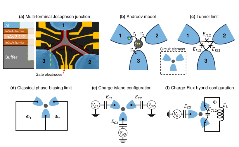
Figure 1: (a) Possible implementation of the trijunction in a hybrid superconductor/semiconductor heterostructure. An aluminium film epitaxially grown on top of a 2DEG (pale orange) induce superconductivity by proximity. The 2DEG can be patterned by a defining a mesa and the junctions are created by etching the Al in some regions (indicated with red lines). The gate electrodes confine the electrons of the 2DEG in the center and control the coupling with each lead. (b,c) Models describing the trijunction. The circuit element indicated with dashed line represents both limits in (d-f). In (b), the middle region is relevant to describe how electrons move between leads. In this work, we use a single level quantum dot in the infinite gap regime at even parity, such that the relevant processes involve the exchange of Cooper pairs between the dot and the leads. In (c), the system is described by effective tunneling processes of single Cooper pairs between the leads -equivalent to 3 tunnel Josephson junctions forming a triangle-, and may reproduce the model in (b) under certain limits. (d-f) Three circuits we consider with the trijunction element. In (d), the phase is externally fixed by the external fluxes $\Phi_{1,2}$. In (e), the trijunction connects three superconducting islands with charging energies $E_{C\nu}$. In (f), two leads form a loop with finite inductance $L$, threaded by flux $\Phi$, and the third lead is a superconducting island.

More generally, from a mesoscopic perspective, a tunnel junction is just a particular case of a weak link between two superconductors [3]. The coupling being weak, bound states with phase-dependent energies form to accommodate the phase difference between both terminals [4, 5, 6]. Solving the energy spectrum of the so-called Andreev states of this SXS device means the diagonalization of the Bogoliubov-deGennes (BdG) Hamiltonian, i.e. a fermionic problem which requires a microscopic model for the X region. In this BdG description, the phase is a parameter determined by the circuit where the weak link is embedded, an approach justified when the phase fluctuations are small and the energy corresponding to the circuit levels is large compared to the Andreev states.

The hybrid situation involving a mesoscopic junction where the phase has to be considered as an operator associated with the transfer of charge has acquired interest with the recent realizations of quantum circuits containing Josephson junctions made out of InAs-nanowires and 2DEGs [7, 8, 9, 10, 11]. These junctions may operate away from the tunneling regime and are better described in terms of high transmission conduction channels or with a quantum dot model. The number of channels, the barriers and chemical potentials can be tuned using gates, thus enabling the realization of devices where the control of the junction parameters is critical. Previous works have already considered this Josephson-Andreev regime at different degrees of approximation, both in the situation with topological leads, where the fermionic levels correspond to Majorana states [12, 13, 14, 15, 16, 17, 18], and with trivial Andreev states [19, 15, 20, 21, 22].

These devices open up the possibility to design hybrid modes combining the fermionic structure of the weak link with the bosonic excitations associated to the electromagnetic collective modes. This is in line with nowadays efforts towards the physical realization of protected qubits, based on the concept of a disjoint support of the qubit wavefunction, which enjoy protection against decoherence from one or more noise sources [23, 24, 25, 26]. Such strategy has been pursued using multimode circuits with conventional junctions [27, 28, 29, 30, 31, 32, 33, 34, 35, 36, 37], mesoscopic junctions where the effect of the Andreev structure is approximated with a modified Josephson potential [38, 39, 40, 41, 42, 43, 44, 45], and mesoscopic junctions where the treatment of the full Andreev structure is essential, as is the case of a quantum-dot with a level in resonance with the Fermi level of the superconducting leads [7, 10, 20, 21, 22].

In this work we explore the properties of multiterminal Josephson-Andreev junctions when immersed in different kinds of quantum circuits (see Fig. 1). These are unique mesoscopic components where the weak-link connects several superconducting leads that have become experimentally accessible in proximitized 2D structures [46]. Since there are several phase difference variables which mimic the k-space in a solid, there has been considerable interest in multiterminal Josephson devices driven by the possibility of engineering topologically protected singularities in their spectrum [47, 48, 49, 50, 51, 52, 53, 54, 55, 56, 57, 58] and, broadly, other applications that arise from the introduction of additional leads [59, 60, 61, 62, 63, 64, 46, 65, 66, 67, 68, 69, 70, 71, 72, 73]. We find that, just at the level of a triterminal junction (Fig. 1a), the presence of a third lead introduces an additional degree of freedom that allows to define protected qubits.

At a more fundamental level, quantum circuits with Josephson-Andreev junctions pose basic questions on the proper quantization rules that determine the system Hamiltonian in a general, time dependent situation. For instance, if an external flux constrains the phases of some circuit elements, the phase drop distribution between and within these elements is not a gauge freedom as in the static situation. The actual drop has to be determined by the electromagnetic field established in the circuit, which depends on its structure and geometry [74, 75, 76, 77, 78] and on the currents spatial distribution [79, 80, 81, 82, 83, 84]. In addition, the circuit variables bear a different nature depending on the configuration of the circuit, leading to continuous or discrete charge variables [85, 86, 87, 88, 89, 90, 91, 92, 93, 94, 95]. In the present work we analyze this problem for different circuit configurations and show its impact on the relaxation rates.

The work is organized as follows: in Section II, we introduce possible experimental implementations and discuss the modelling of the junction with a single level between the leads (Fig. 1b), its embedding in a phase biased configuration (Fig. 1d) and the effect of the phase drop distribution on the relaxation rates. In Section III, we consider a circuit where the leads are superconducting islands (Fig. 1e) and discuss a transmon-like regime that hosts two almost degenerate states. In section IV, we connect two leads in a loop with finite inductance with a third one which is an island (Fig. 1f) and discuss a regime simultaneously protected against charge and flux noise. Lastly, in section V, we describe the tunnel limit of a multiterminal junction (Fig. 1c) and its connection to protected multimode circuits designed with several conventional elements.

II Modelling, phase biased configuration and gauge choice

The basic element that we consider as a building block for quantum circuits is the Josephson-Andreev trijunction. As illustrated in Fig. 1(a), it consists of a normal central region coupled to three superconducting leads. Such a device can be implemented on a proximitized two-dimensional electron gas (2DEG) defined, for instance, on a Al/InAs heterostructure [96, 11, 97, 98, 99]. We assume that the charge density in the normal region can be controlled by gates and that a situation where a few or just one conduction channel on each terminal can be reached. In such situation the Josephson coupling between the leads is mediated by a few Andreev bound states, sensitive to the phase on each superconducting contact. Notice that in the configuration of Fig. 1(d) two well defined phase differences between the leads can be controlled by external fluxes $\Phi_{1,2}$ through the corresponding loops, as indicated in the figure. Within this section, we assume ideal phase biasing, i.e. loops without inductance and negligible charging energy.

As commented in the introduction, determining the Andreev spectrum for such geometry requires solving the BdG equations with the corresponding boundary conditions for the superconducting phases. This is, in general, a formidable task that can be undertaken using different models and numerical techniques. For the purpose of the present work, however, we adopt several simplifying assumptions that enable a tractable but still realistic description of the device.

Assuming a single channel per lead and that the dimensions of the normal region are short compared to the superconducting coherence length, we describe it in terms of a single level model. We denote by $d^{\dagger}_{\sigma}$ the operator creating an electron with spin $\sigma$ in that level. In addition, we describe the leads in the so-called infinite-gap limit, which allows us to include their effect in the normal region as a frequency independent pairing self-energy [100, 101, 102]. The effective Hamiltonian for the trijunction is given by (see Appendix A)

$$H^{\rm eff}=\sum_{\sigma}\epsilon n_{\sigma}+Un_{\uparrow}n_{\downarrow}+\sum_{\nu=1}^{3}\left[\Gamma_{\nu}e^{-i\phi_{\nu}}d^{\dagger}_{\uparrow}d^{\dagger}_{\downarrow}+\mbox{h.c.}\right]\;,$$ (1)

where $\epsilon$ is the position of the central level referred to the leads chemical potential, $U$ is its charging energy, and $\Gamma_{\nu}$ is the tunneling rate to the lead $\nu$, which has a phase $\phi_{\nu}$.

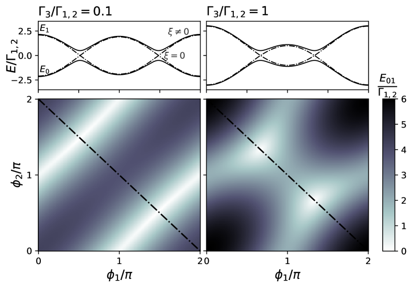
Figure 2: Bottom: Transition energy $E_{01}$ versus the phase differences $\phi_{1,2}$ for $\Gamma_{1}{=}\Gamma_{2}$ and different $\Gamma_{3}$. At low coupling $\Gamma_{3}$ (left), the system roughly behaves as a junction between $1$ and $2$, and depends on the phase difference $\phi_{1}-\phi_{2}$ between them. At comparable couplings $\Gamma_{1,2,3}$ (right), the transition landscape has a set of local minima. The level position is placed at the symmetry point $\epsilon{=}-U/2$, meaning $\xi{=}0$. Top: energies $E_{0,1}$ (up to a shift) of the Andreev states along the trajectories highlighted in the maps, with solid (dash-dotted) lines for $\xi{=}0.5$ ($\xi{=}0$).

Such model is characterized by a phase diagram with alternating even and odd parity ground states as a function of the model parameters [102, 103, 104, 50, 105, 58]. However, as in the present work we focus on the case of widely open channels with significant Josephson coupling, we assume that the trijunction remains always within the even sector, where $H^{\textrm{eff}}$ is projected as

$$H^{\textrm{eff}}_{\textrm{even}}=-\xi\tau_{z}+\xi+\sum_{\nu}\Gamma_{\nu}(\cos{\phi_{\nu}}\tau_{x}-\sin{\phi_{\nu}}\tau_{y}),$$ (2)

with $\xi=\epsilon+U/2$ and $\tau_{i}$ the Pauli matrices acting on the space $\{\ket{0}_{d},\ket{\uparrow\downarrow}_{d}\}$. The ground and excited states have energies

$$E_{0,1}(\{\phi_{\nu}\})=-\xi\mp\sqrt{\xi^{2}+\bigg{|}\sum_{\nu}\Gamma_{\nu}e^{-i\phi_{\nu}}\bigg{|}^{2}}\;.$$ (3)

Let us note that, while $H^{\rm eff}$ in Eq. (1) does depend on the phase gauge choice, its spectrum (3) is only sensitive to the phase differences so for simplicity we take $\phi_{3}=0$. The transition energy $E_{01}=E_{1}{-}E_{0}$ is shown in Fig. 2 (bottom) for $\Gamma_{1}=\Gamma_{2}$ and different ratios $\Gamma_{3}/\Gamma_{1,2}$. When the lead $3$ is weakly coupled (left panel), the energy depends mainly on the phase difference between the two strongly coupled leads, $\phi_{2}{-}\phi_{1}$, which at $\pi$ corresponds to a minimum in $E_{01}$. When the three leads are equally coupled (right panel), the landscape reveals a discrete set of extrema and saddle points. In the regime $\Gamma_{3}\gg\Gamma_{1,2}$, the phase dependence is weaker and there is a minimum in $E_{01}$ at $\phi_{1,2}\approx\pi$. On the top of Fig. 2, the Andreev energies $E_{0,1}$ corresponding to the trajectories in the $(\phi_{1},\phi_{2})$ plane indicated in the bottom panels are shown in dash-dotted (solid lines) for $\xi=0$ ($\xi=0.5$), that is, in (out of) resonance with the dot level. These energies are plotted with a $-\xi$ shift.

This two-level system would be an instance of an Andreev level qubit [106, 107], a kind of qubit defined with two Andreev states of a junction [108, 109, 110], and the choice of its operating point should consider aspects such as its sensitivity to noise. The noise in some parameter $\lambda$ produces decoherence through two mechanisms, pure dephasing and depolarization [111]. On the one hand, pure dephasing relates with the change in the qubit energy, blurring the access to the phase of superpositions of the type $c_{0}\ket{0}+c_{1}e^{i\varphi}\ket{1}$, $c_{0,1}{\in}\mathbb{R}$. For small noise amplitudes, the associated rate $T^{-1}_{\varphi}(\lambda)$ is proportional to $|\partial E_{01}/\partial\lambda|^{2}$. On the other hand, depolarization relates to the relaxation from $\ket{1}$ to $\ket{0}$, and at small amplitudes the associated rate $T^{-1}_{1}(\lambda)$ is proportional to $|\bra{0}\partial H/\partial\lambda\ket{1}|^{2}$. Several strategies aim at reducing the effect of the noise: reducing its amplitude, correcting errors, or designing the qubit such that it acquires an inherent protection [23]. The latter approach can be explored when introducing different hardware configurations, attempting to reduce the dephasing and the depolarization rates simultaneously. This is not a straightforward task and it must be noticed that simultaneous protection against noise in all parameters is impossible. In conventional qubits the noise in the charge offset and the external flux are the dominant ones and the noise in the Josephson coupling in a transmon is much lower [112, 111, 113]). In the circuits we consider here, the couplings can be controlled by gate voltages, so the associated noise may not be negligible. However, for simplicity and to illustrate the principle, throughout this work we focus on the noise in the external flux, in the energy of the dot level and in the charge offset of the superconducting islands introduced in Sec. III.

II.1 Noise protection of the Andreev qubit

The general challenge for the simultaneous reduction of dephasing and depolarization produced by noise in one parameter can be illustrated in the phase biased configuration of the present section. For example, the noise in $\xi$ has a dephasing sweet spot at $\xi=0$, where $E_{01}(\xi)$ is locally quadratic. However, at this spot the hybridization between the bare central level states $\ket{0}_{d}$ and $\ket{\uparrow\downarrow}_{d}$ is enhanced, so the relaxation rate increases (note that $\partial H^{\textrm{eff}}/\partial\xi\propto\tau_{z}$ and the states are $\propto\ket{0}_{d}\pm\ket{\uparrow\downarrow}_{d}$). The same occurs with the noise in the external flux, which has dephasing sweet spots where two states which were degenerate become hybridized. In the two terminal case, it occurs in the configuration of perfect transmission ($\xi{=}0$ and $\Gamma_{1}{=}\Gamma_{2}$ [20], see top panels of Fig. 2) at phase difference $\phi_{e}=\pi$, where the two degenerate states carry maximal and opposite supercurrents. There, a deviation in the energy level position or in the coupling symmetry hybridizes these states while flattening the transition energy at the same time. As will be discussed next, this analysis on the effect of flux noise must be extended to take into account the effect of the phase drop distribution.

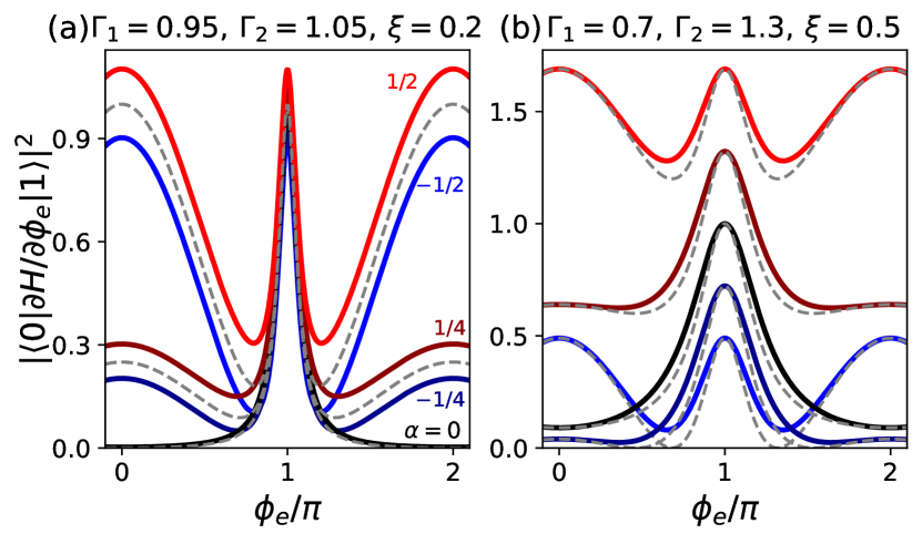
Figure 3: Phase dependence of the transition matrix elements for different phase drop distributions in a junction with two leads: symmetrically over the couplings ($\alpha{=}0$), on $\Gamma_{1}$ ($\alpha{=}-1/2$), on $\Gamma_{2}$ ($\alpha{=}1/2$) and halfway ($\alpha{=}\mp 1/4$). (a) Situation close to resonance. Low but finite deviation from $\xi{\neq}0$ and $\Gamma_{1}{\neq}\Gamma_{2}$ produces the high peak at $\delta{=}\pi$ due to the anticrossing between $E_{0}$ and $E_{1}$ (see Fig. 2 top). The slight asymmetry in the couplings produces asymmetry over the sign of $\alpha$ (grey dashed lines show the results for $\Gamma_{1,2}{=}1$). (b) Situation with larger coupling asymmetry, producing a large asymmetry over the sign of $\alpha$; dashed lines show the results for $\xi{=}0$.

In a static situation, the phases in Eq. (2) have a gauge freedom which manifests through the transformation $U{=}e^{if\tau_{z}/2}$, where the phase $f$ redistributes the phase drop over the couplings. In fact, note that the coupling term of $H^{\textrm{eff}}_{\textrm{even}}$ in Eq. (2) can be written as $\sum_{\nu}\Gamma_{\nu}e^{i\phi_{\nu}\tau_{z}/2}\tau_{x}e^{-i\phi_{\nu}\tau_{z}/2}$, so the transformed coupling term in $UH^{\textrm{eff}}_{\textrm{even}}U^{\dagger}$ corresponds to a shift $\phi_{\nu}\rightarrow\phi_{\nu}+f$. However, if the external fluxes depend on time, such as in a situation with noise, the transformation adds to the new Hamiltonian the term $-i\hbar U(U^{-1})^{\prime}=-\hbar f^{\prime}\tau_{z}/2$, where the prime indicates time derivative and $f$ might depend on the internal and external parameters of the circuit. This non-equivalence means that a Hamiltonian with no term $\propto f^{\prime}\tau_{z}$ would only be correct at a certain gauge choice [74, 75]. Classically, the magnetic vector potential $\vec{A}$ –which determines the quantum phase drop through a Peierls substitution– may be shifted by the gradient of a scalar function $F$ without altering the magnetic field, but if $F$ is time dependent, the complete gauge transformation must subtract $\partial_{t}F$ from the scalar potential $V$ –which determines a voltage profile– so that the electric field $\vec{E}=-\vec{\nabla}V-\partial_{t}\vec{A}$ is not modified.

The simplest way to notice this effect is in the flux noise matrix element of a junction with two leads. In this case, the general form of the coupling term in $H^{\rm eff}_{\rm even}$ is

$$(\Gamma_{1}\cos{(-\phi_{e}/2{+}f)}+\Gamma_{2}\cos{(\phi_{e}/2{+}f)})\tau_{x}$$

$$-(\Gamma_{1}\sin{(-\phi_{e}/2{+}f)}+\Gamma_{2}\sin{(\phi_{e}/2{+}f)})\tau_{y},$$

where $f$ determines how asymmetrically this phase drops on the couplings between the leads and the dot. Supposing that this asymmetry is proportional to the phase drop, i.e. $f=\alpha\phi_{e}$, which would include terms $\propto\phi_{e}^{\prime}\tau_{z}$ in the Hamiltonian for a general gauge, the squared matrix element $|\bra{0}\partial H/\partial\phi_{e}\ket{1}|^{2}$ is

$$\frac{(\Gamma_{1}^{2}{+}\Gamma_{2}^{2}{+}\xi^{2})^{2}{-}4\Gamma_{1}^{2}\Gamma_{2}^{2}}{E_{01}^{2}}{-}\frac{\xi^{2}}{4}{+}\alpha(\Gamma_{2}^{2}{-}\Gamma_{1}^{2}){+}\alpha^{2}\left(\frac{E_{01}^{2}}{4}{-}\xi^{2}\right),$$

which is illustrated in Fig. 3. In panel (a), the couplings are almost symmetric and the matrix element depends slightly on the sign of $\alpha$ (the grey dashed lines correspond to the limit of $\Gamma_{1}{=}\Gamma_{2}$). In panel (b), the couplings are less symmetric and the sign of $\alpha$ has a strong effect reducing or boosting the relaxation (the grey dashed lines correspond to the limit of $\xi{=}0$). The matrix element at $\phi_{e}{=}\pi$ vanishes at $\alpha_{0}=(\Gamma_{1}{+}\Gamma_{2})/2(\Gamma_{1}{-}\Gamma_{2})$, a regime approached in the fully asymmetric phase-drop distribution $\alpha{=}{\pm}1/2$ at large coupling asymmetry. However, the value $\absolutevalue{\alpha_{0}}{\geq}1/2$ requires that the phase drop winds more than once, an unlikely situation in a superconducting loop where vortices would appear to accommodate the next flux quantum whenever the phase surpasses $2\pi$ [114, 115, 116]. The value at $\phi_{e}{=}\pi$ becomes a local minimum at $\alpha_{m}$, with $2\alpha_{m}^{2}=(\xi^{2}{+}(\Gamma_{1}{+}\Gamma_{2})^{2})/(\xi^{2}{+}(\Gamma_{1}{-}\Gamma_{2})^{2})$, with $\absolutevalue{\alpha_{m}}\geq 1/2$ too.

The calculation of the particular $f$ value appropriate for each configuration requires to know the electromagnetic field distribution in the circuit [74, 75, 76], which is out of the scope of the present work. Our aim here is to identify the main features that determine it: the shape of the field in the central part of the junction depends on the geometry and properties of the circuit in which it is immersed [77], though in the situation we consider here we expect little variation in the field profile as the central region is small compared to a typical field wavelength and presumably homogeneous, i.e. we expect a symmetric drop of the phase difference. However, the state of the junction might carry a supercurrent, which modifies the field. A calculation in the lines of [79] (see Appendix A), which imposes electroneutrality in the electrodes, produces a deviation from the symmetric drop with $f{=}-\sum_{\nu}\Gamma_{\nu}\phi_{\nu}/\Delta$, where $\Delta$ is the superconducting gap. In the two terminals setup, it gives $\alpha=(\Gamma_{1}-\Gamma_{2})/\Delta$, which vanishes in the limit of large gap.

In the setup with three leads (Fig. 1d), the coupling term (Eq. (2)) is

$$\Big{[}\Gamma_{1}\cos{(-\phi_{e1}/2{+}f)}+\Gamma_{2}\cos{(\phi_{e2}/2{+}f)}+$$

$$\Gamma_{3}\cos{(\phi_{e1}/2{-}\phi_{e2}/2{+}f)}\Big{]}\tau_{x}-\Big{[}\cos{\rightarrow}\sin]\tau_{y},$$

which in the limit $\Gamma_{3}{\rightarrow}0$ is not equivalent to the two leads case: if the fluxes have the same source and obey $\phi_{1,2e}=\eta_{1,2}\phi_{e}$, then $f=(\Gamma_{1}\eta_{1}-\Gamma_{2}\eta_{2})\phi_{e}/2$. For $\eta_{1,2}=1$, we have the same Hamiltonian as in the two leads case, but now the phase drops $-\phi_{e}/2{+}(\Gamma_{1}{-}\Gamma_{2})\phi_{e}/2$ and $\phi_{e}/2+(\Gamma_{1}-\Gamma_{2})\phi_{e}/2$ (which involve the couplings between the leads that form loops) can go up to $2\pi$, therefore becoming able of achieving the relaxation free point $\alpha_{0}$ for parameters where $1/2\leq\absolutevalue{\alpha_{0}}\leq 1$.

We note that there are other transformations $U_{n}{=}e^{if_{n}\tau_{n}}$ ($n{\neq}z)$ that generate the time dependent terms $-\hbar f_{n}^{\prime}\tau_{n}/2$. The case $n{=}0$ ($\tau_{0}{=}\mathbbm{1}$) refers to a global energy shift and introduces a global time dependent phase with no effects. The cases $n{=}x,y$ have no apparent physical interpretation, but the time dependent term must be kept if the transformation has been made for example to facilitate calculations.

As argued in the previous paragraphs, the phase drop distribution is very important for the relaxation rates. In addition, from a broader perspective, its effect is pervasive on other observable quantities that depend on the matrix elements, such as the shift of a resonator coupled to the circuit or the transition rates between the states in the junction [117, 118, 119, 120, 121, 122, 123, 124].

II.2 Topological properties

This model of the trijunction in a perfect phase-biasing configuration can be linked with the topological singularities predicted in general multiterminal junctions [47], since there are certain configurations where $E_{01}$ reaches $0$, forming a Weyl point. In our case (see Eq. (3)), these points appear when the parameter $\xi$ and the sum $\Gamma_{T}=\sum_{\nu}\Gamma_{\nu}e^{i\phi_{\nu}}$ vanish, so topological protection in this model against variations in $\xi$ is not possible, though it is on the $\Gamma_{\nu}$. It is convenient to interpret $\Gamma_{T}$ as a vector in the complex plane, formed by the addition of the constituent numbers of magnitude $\Gamma_{\nu}$ and direction $e^{i\phi_{\nu}}$. In the case of two terminals, the only possibility is $\Gamma_{1}=\Gamma_{2}$ with a phase difference of $\pi$. However, with three terminals, if the $\Gamma_{\nu}$ satisfy the triangle inequality (each side is smaller than the sum of all the other sides) there is a set of phase differences that produce a Weyl point – a similar argument has been recently used to map a general model of a multiterminal quantum dot Josephson junction into a two terminal one [58]. In this case, the Weyl points would be protected against variations on the $\Gamma_{\nu}$, as long as they continue satisfying the triangular equality. If the number of terminals is increased to $\mathcal{N}$, the generation of Weyl points becomes more probable since there are more ways of closing a polygon with $\mathcal{N}$ sides, and they live in a phase space of $\mathcal{N}-1$ dimensions.

This configuration can be compared to a multiterminal junction in the tunnel limit, with $H=\Re{\sum_{\mu>\nu}E_{J_{\mu\nu}}e^{i(\phi_{\mu}-\phi_{\nu})}}$. In this case there is only one “band” but the points where $H=0$ are interesting as they correspond to a maximum supercurrent, and the $E_{J_{\mu\nu}}$ play a role similar to that of the $\Gamma_{\nu}$ for defining these points.

III Charge islands configuration

In this section we consider the situation in which the central region is connected to isolated superconducting islands (Fig. 1e). In this configuration the number of Cooper pairs in each island $N_{\nu}$ is a discrete variable and the total number of pairs $N_{T}=\sum_{\nu}N_{\nu}+n_{d}$ is conserved, where $2n_{d}$ is the number electrons in the central region. This conservation constrains the accessible states in the basis $\ket{\{N_{\nu}\},n^{\alpha}_{d}}$ for a given value of $N_{T}$, where the $\ket{n^{\alpha}_{d}}$ are the states in the central region. In our model, we only consider $\ket{0}_{d}$ ($n_{d}{=}0$) and $\ket{\uparrow\downarrow}_{d}$ ($n_{d}{=}1$), with $\hat{n}_{d}=\sum_{\sigma}d^{\dagger}_{\sigma}d_{\sigma}/2$, so the label $\alpha$ will be dropped from now on. As a result of the constraint, an instance of $N_{T}$ can be described with a smaller basis, i.e. one lead variable can be removed using $\hat{N}_{\mu}=N_{T}-\sum_{\nu\neq\mu}\hat{N}_{\nu}-\hat{n}_{d}$.

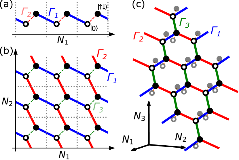
Figure 4: Lattice representation of the island configuration. The island charge variables $N_{\nu}$ define the dimensions of the crystal and the fermionic states are the atoms in the unit cell, with hollow (full) circles for $\ket{0}$ ($\ket{\uparrow\downarrow}$). The sets of connected states for an instance of total charge $N_{T}$ are the blue dimers (a), the blue-red chains in (b) and the blue-red-green grid in (c) for the setups of 1, 2 and 3 leads, respectively. The dashed lines represent the projection of a single instance in a space with lower dimension, where the projected variable is determined by the conservation of $N_{T}$, e.g. a blue-red chain in (a), where $N_{2}=N_{T}-N_{1}-n_{d}$. The pale circles in (c) represent sites of adjacent $N_{T}$ grids, which would be connected in the presence of a fourth lead.

The charging effects in and between the islands are described by a capacitance matrix $\mathcal{C}$ such that the associated Hamiltonian is $H_{C}=(\vec{N}-\vec{n}_{g})^{T}\mathcal{C}^{-1}(\vec{N}-\vec{n}_{g})$, where $\vec{N}=(\hat{N}_{1},\hat{N}_{2},...,\hat{N}_{\mathcal{N}})$ is the vector of the number operators in each of the $\mathcal{N}$ islands and $\vec{n}_{g}$ includes the corresponding effective charge offsets, which indicate the charge configuration in a situation of electrostatic equilibrium. In general, $H_{C}$ can be interpreted as a confining potential in the charge basis, and it could also include capacitive couplings between the leads and the central region by increasing its size and including $\hat{n}_{d}$ in $\vec{N}$. The particular values of $\mathcal{C}$ depend on how the electromagnetic field accommodates into the geometry and materials of the device. We consider the regime where the absolute charge offsets are large enough so that the eigenspectrum of the $\hat{N}_{\nu}$’s can be extended to $N_{\nu}\in\mathbb{Z}$ (the $n_{g_{\nu}}$’s are shifted to denote deviations from the integer set closest to equilibrium).

As discussed in [20], deep inside the gap and restricted to the even parity sector, the main tunneling process is the effective interchange of Cooper pairs between the leads and the central level, though microscopically the electrons actually tunnel one by one [15]. Thus, in the infinite gap limit discussed in the previous section, the coupling Hamiltonian is $H_{c}=\sum_{\nu}\Gamma_{\nu}e^{-i\hat{\phi}_{\nu}}d^{\dagger}_{\uparrow}d^{\dagger}_{\downarrow}+h.c.$, where $e^{-i\hat{\phi}_{\nu}}$ decreases $N_{\nu}$ by $1$ (now the phase is the generator of the charge translations with $[\hat{\phi}_{\mu},\hat{N}_{\nu}]=i\delta_{\mu\nu}$), and $d^{\dagger}_{\uparrow}d^{\dagger}_{\downarrow}$ introduces both electrons of the pair in the dot. The $N_{T}$ constraint in the Hilbert space $\ket{\{N_{\nu}\},n_{d}}$, which can be described by a gauge symmetry in the phase space [20, 14], may be noticed by the fact that the states $\ket{\{N_{\nu}\},0}$ and $\ket{\{N_{\nu}\},\uparrow\downarrow}$ are not connected in any way – for the coupling conserves the total charge. However, these states are hybridized when an additional island is introduced – this is the main feature explored in this section.

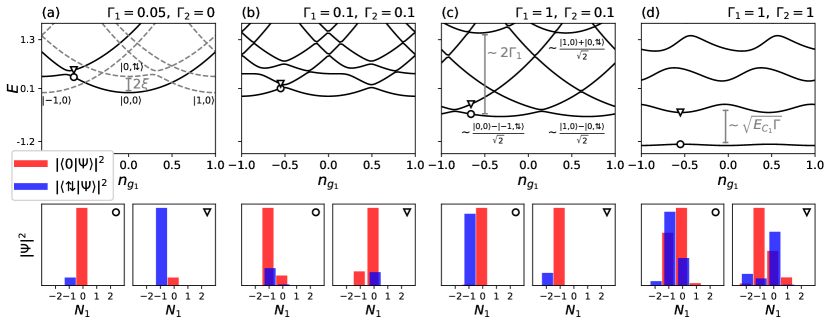
Figure 5: Energy dispersion over the charge offset $n_{g_{1}}$ in the configurations with 1 and 2 terminals ($E_{C_{1}}=1$, $E_{C_{2}}=0$, $\xi=0.2$), and wavefunctions indicated with markers (bottom panels). (a) Small coupling of the central level with island $1$: the instance $N_{T}{=}0$ is in solid lines, and other instances in dashed; some bare $\ket{N_{1},n_{d}}$ states are indicated close to the bottom of their charging parabolas. (b) Small couplings with islands $1$ and $2$: finite $\Gamma_{1}$ and $\Gamma_{2}$ connect all states in (a). (c) Large (small) coupling with terminal $1$ ($2$): $\Gamma_{1}$ dominates the formation of symmetric and antisymmetric combinations. (d) Large couplings (similar to a transmon except that the junction is close to resonance, not in the tunnel regime).

If the basis is portrayed as a lattice in the $\{N_{\nu}\}$ space with a unit cell comprising the fermionic levels, each $N_{T}\in\mathbb{Z}$ constitutes an independent set disjoint from the others (see Fig. 4). Starting with one island and the central level, these sets are the groups of two sites fulfilling $N_{1}+n_{d}=N_{T}$ (the dimers connected with blue lines in Fig. 4a). Then, when the second island is coupled, the sets are 1D chains defined by $N_{1}+N_{2}+n_{d}=N_{T}$ (the blue and red chains in Fig. 4b). One of these instances of $N_{T}$ is projected on panel (a), where the dashed red lines represent the coupling $\Gamma_{2}$ and $N_{2}=N_{T}-N_{1}-n_{d}$. When a third lead is connected, the chains connect between themselves through $\Gamma_{3}$ and form a 2D grid fulfilling $N_{1}+N_{2}+N_{3}+n_{d}=N_{T}$, depicted in Fig. 4c and projected to $N_{1,2}$ in panel (b). Similarly, these grids may be connected when a 4th lead is included, and so on. In the following subsections, this kind of circuits is progressively explored along with some applications for the definition of protected qubits.

III.1 One terminal

We consider first a single superconducting island with $H_{C}=E_{C_{1}}(\hat{N}_{1}{-}n_{g_{1}})^{2}$ connected to the central region. The relevant states $\ket{N_{1},n_{d}}$ are

$$\ket{0,0}\rightarrow E =E_{C_{1}}n_{g_{1}}^{2}$$

$$\ket{-1,\uparrow\downarrow}\rightarrow E =E_{C_{1}}(-1-n_{g_{1}})^{2}+2\xi,$$ (4)

where a translation in $N_{1}{=}N_{T}$ would refer to other instances of total charge (blue dimers in Fig. 4a). The energies of the $N_{T}{=}0$ instance ($n_{g_{1}}$ is shifted so that it refers to the lowest energy instance) are the solid black parabolas in Fig. 5a, hybridized by the tunneling $\Gamma_{1}$, which opens an anticrossing at $n_{g_{1}}{=}-1/2-\xi/E_{C_{1}}$ (close to the symbols that indicate the wavefunctions in the lower panels). The dashed lines in Fig. 5a represent other instances of $N_{T}$, which are in principle uncoupled sub-spaces.

As indicated in the lower panels, the two-level system in the limit $\Gamma_{1}\ll E_{C}$ is similar to a charge qubit with a steep $n_{g}$ dependence that would be detrimental for coherence in the presence of noise. In the opposite limit $\Gamma_{1}\gg E_{C}$, the eigenstates are the symmetric and antisymmetric combinations $\ket{N_{1}^{\prime},\pm}{=}(\ket{N_{1},0}{\pm}\ket{N_{1}{-}1,\uparrow\downarrow})/\sqrt{2}$, for a larger range in $n_{g}$, with a transition energy $\sim 2\Gamma_{1}$. The dispersion of $E_{01}$ over $n_{g}$ is reduced (${\sim}E_{C_{1}}n_{g_{1}}^{2}/\Gamma_{1}$), but now the relaxation produced by the noise in $n_{g}$ is larger as $\partial H/\partial n_{g_{1}}$ is non-diagonal in the qubit basis. When compared with the transmon, this setup does not suffer the problem of reduced anharmonicity, but we note that the single level model of Eq. (1) would not be valid at arbitrary $\Gamma_{1}$ because $\ket{0}$ and $\ket{1}$ could approach other levels in the central region.

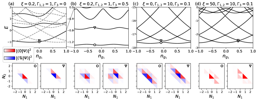
Figure 6: Energy dispersion over the charge offset $n_{g_{1}}$ in the configurations with 2 and 3 terminals when two of them are islands with charging energy $E_{C_{1}}=1=E_{C_{2}}$ (setting $n_{g_{2}}=0$) and wavefunctions indicated with markers, represented in a $N_{1}$-$N_{2}$ space where each cell is divided into a lower and an upper triangle for the level states $\ket{0}$ and $\ket{\uparrow\downarrow}$, respectively (bottom panels) (a) Only two terminals as in Fig. 5d but now the terminal $2$ has finite charging energy, which renders the spectrum aperiodic and non-equivalent between instances ($N_{T}{=}0$ in solid lines, others in dashed). (b) Introducing the coupling $\Gamma_{3}$ with the third terminal, which connects the different instances (chains) in (a). (c) Large couplings $\Gamma_{1,2}$ (transmon regime in the $N_{1}{-}N_{2}$ direction) and small coupling $\Gamma_{3}$ (Cooper pair box regime in the orthogonal direction), central level close to resonance. (d) Same with central far from resonance (tunneling regime).

III.2 Two terminals

When a second terminal is connected to the central region, the constraint $N_{1}+N_{2}+n_{d}=N_{T}$ produces independent sets with an infinite number of states, the blue and red chains in Fig. 4b. In the extended basis $\ket{N_{1},N_{2},n_{d}}$, the coupling $\Gamma_{2}$ (red) connects $\ket{0,0,0}$ with $\ket{0,-1,\uparrow\downarrow}$, which in the projected basis $\ket{N_{1},n_{d}}$ appears as a coupling between $\ket{0,0}$ with $\ket{0,\uparrow\downarrow}$ (red dashed lines in Fig. 4a). To illustrate this we start by considering that the second terminal is floating and very large so there is no additional charging energy.

In this situation, we have $H_{C}=E_{C_{1}}(\hat{N}_{1}{-}n_{g_{1}})^{2}$, and in the limit $\Gamma_{1,2}\ll E_{C_{1}}$, the states (in the reduced basis) $\ket{0,0}$ and $\ket{-1,\uparrow\downarrow}$ maintain the anticrossing given by $2\Gamma_{1}$ as in the previous subsection. The coupling $\Gamma_{2}$ does not directly open anticrossings between $\ket{N_{1},0}$ and $\ket{N_{1},\uparrow\downarrow}$, because their energies never coincide. However, at $n_{g_{1}}{=}{-1/2}$ (indicated by symbols in Fig. 5b) both couplings combine to hybridize $\ket{N_{1}{-}1,n_{d}}$ with $\ket{N_{1},n_{d}}$ through an intermediate state with opposite central level occupation. For finite $\absolutevalue{\xi}\gg\Gamma_{1,2}$ the gap opening is $\sim(\Gamma_{1}^{2}+\Gamma_{2}^{2})/\xi$. The states $\ket{N_{1}{-}1,0}$ and $\ket{-1,\uparrow\downarrow}$ also hybridize through two intermediate states at $n_{g_{1}}{\approx}-1/2+\xi/E_{C_{1}}$, with an even smaller anticrossing (the size decreases with the number of intermediate states needed for the indirect coupling). In the lower panels we show the different states $|N_{1}\rangle$ contributing to the ground and the first excited eigenstates. As we discuss next, more and more charge states contribute as the coupling is increased.

In the limit $\Gamma_{1}{\gg}E_{C_{1}}{\gg}\Gamma_{2}$ (corresponding qualitatively to Fig. 5c), the lowest energy states ${\sim}\ket{N_{1}^{\prime},-}$ and ${\sim}\ket{N_{1}^{\prime}{+}1,-}$ anticross close to $n_{g_{1}}{=}N_{1}$ opening a gap ${\sim}\Gamma_{2}$. Note that these two levels are completely disjoint at $\Gamma_{2}{=}0$, defining a qubit protected against relaxation. However, as discussed in the previous subsection, the decoherence produced by the noise in $n_{g_{1}}$ may be important for feasible values of $\Gamma_{1}$.

We address now the regime $\Gamma_{1,2}{\gg}E_{C_{1}}$ in which the wavefunctions extend broadly over the charge states (Fig. 5d), thereby decreasing the modulation produced by the offset charge $n_{g_{1}}$, just like in the transmon [113]. The Josephson-Andreev junction should recover the typical tunnel junction transmon when the central level is far from resonance. In this case there is an exponential suppression of the charge dispersion with $E_{J}^{\textrm{eff}}/E_{C_{1}}$, where $E_{J}^{\textrm{eff}}$ is the effective amplitude of Cooper pair tunneling between the leads [113]. In the resonant limit, the Josephson-Andreev transmon (JAmon) dispersion is even more suppressed and becomes dominated by the tunneling of pairs of Cooper pairs [20]. In either case, the dispersion is a non-perturbative effect.

In order to estimate the levels energies, we may disregard this dispersion and use an adiabatic approximation in the phase space, which consists in using the phase dependence $E_{0}(\phi_{e})$ (Eq. (3)) of the Andreev lowest state as the effective potential in the phase variable $\phi_{e}\rightarrow\hat{\phi}_{1}$. Then, in the transmon-like limit of localized phase, it is expanded up to $\textrm{4}^{\textrm{th}}$ order at $\phi_{e}{=}0$ to get the harmonic separation $\omega\approx E_{01}$ between states and the anharmonicity $\alpha{=}E_{12}{-}E_{01}$ at lowest order. In the tunnel limit $\xi{\gg}\Gamma_{1,2}$, $\omega\approx 2\sqrt{E_{C_{1}}\Gamma_{1}\Gamma_{2}/2\xi}$, and in the resonant limit $\delta\Gamma{=}0{=}\xi$, with $\Gamma,\delta\Gamma{=}\Gamma_{1}{\pm}\Gamma_{2}$, $\omega\approx 2\sqrt{E_{C_{1}}\Gamma}$. More details are provided in Appendix B.

Two charge islands

In the situation we have analysed so far, where there is charging energy only in one island, the spectrum is periodic in $n_{g_{1}}$, as a charge translation in $N_{1}$ equals to a charge translation in the charge offset. Moreover, all instances $N_{T}$ are equivalent, because a charge translation in $N_{1}$ also corresponds to a translation in $N_{T}$. This also occurs in the situation where the charging energy only depends on the imbalance between the two islands, with $H_{C}=E_{C_{12}}(\hat{N}_{1}{-}\hat{N}_{2}{-}n_{g_{12}})^{2}$, which has been thoroughly analysed in [20]. However, this is not true in general when the two leads are islands with finite charging energies.

In this case, the additional charging term in the reduced basis,

$$E_{C_{2}}(\hat{N}_{2}{-}n_{g_{2}})^{2}=E_{C_{2}}(N_{T}{-}\hat{N}_{1}{-}\hat{n}_{d}{-}n_{g_{2}})^{2},$$

removes the periodicity in the offset charges and the equivalence between $N_{T}$ instances. This is shown in Fig. 6a, which uses same parameters as in Fig. 5d except for the introduction of $E_{C_{2}}=E_{C_{1}}$ and is similar to the crossover between the one and two leads cases in Fig. 5a, where the solid lines indicate a particular instance (not periodic in $n_{g_{1}}$ now) and the dashed lines indicate different, uncoupled ones.

III.3 Three terminals

When a third terminal is connected to the central region, there are two independent charge variables – we may use for example the projected basis $\ket{N_{1},N_{2},n_{d}}$ where $\hat{N}_{3}=N_{T}{-}\hat{N}_{1}{-}\hat{N}_{2}{-}\hat{n}_{d}$. In this situation, if the charging potential is flat in one direction, the wavefunctions are not constrained and a continuous band is formed in that direction. Considering the charging terms as a quadratic form in the charge variables, then the previous condition occurs when one of its principal axes has a $0$ eigenvalue. Therefore, in order to have a discrete set of states, we consider a fully confining potential. In particular, we select the potential for the situation where two terminals are islands with finite charging energies $E_{C_{1}}$ and $E_{C_{2}}$ (used in the last part of the previous subsection), and the third terminal has no charging energy.

In this case, a finite coupling $\Gamma_{3}$ connects the chains that were independent instances in the case with two terminals (Fig. 6a,b), and the wavefunctions extend in the number space according to the charging potential and the couplings $\Gamma_{\nu}$. When the wavefunctions are broadly extended in charge ($E_{C_{\nu}}\textrm{'s}\ll\Gamma_{\nu}\textrm{'s}$) the system can be thought as a set of coupled harmonic oscillators, a limit which is analyzed in the tunneling regime in Sec. V. Here, we focus in the limit of small $\Gamma_{3}$ compared with the charging energy in the transverse direction of the chains, which suggests the definition of a qubit formed by two adjacent chains (Fig. 6c,d). This limit is better understood in a number basis where one degree of freedom refers to the extension of the wavefunction on the direction of a chain ($N_{1}{-}N_{2}=:N_{12}$, the diagonal in the wavefunction plots in Fig. 6) and the other one refers to the specific chain ($N_{1}{+}N_{2}{+}n_{d}=N_{T}{-}N_{3}$, the antidiagonal). The offset charge does not affect in the chain direction, but in the orthogonal one it produces charge parabolas. In the case $E_{C_{2}}{=}E_{C_{1}}$, illustrated in Fig. 6, the charging potential in that orthogonal direction is $\sim E_{C_{1}}(N_{3}{+}n_{d}{+}N_{T}{+}n_{g_{1}}{+}n_{g_{2}})^{2}/2$. Due to the structure of the wavefunctions in the resonant and tunneling (large $\xi$) limits, where $\langle n_{d}\rangle\approx 0,\,1/2$, respectively (panels c and d), the spectrum has minima in $n_{g_{1}}$ at $\mathbb{Z}{+}1/2$ and $\mathbb{Z}$ when setting $n_{g_{2}}{=}0$. The structure of the wavefunctions also determines the size of the anticrossings, which is $\sim 2\Gamma_{3}$ in the resonant and $\sim\Gamma_{3}^{2}/\xi$ in the tunneling limit.

III.4 Discussion

The lattice picture used in this section of charge islands allows us to relate these systems with the definition of protected qubits that use states of disjoint support. As argued in a recent work that addresses the protection enabled by the resonant regime of a quantum-dot junction in a loop [22] (see Sec. IV.1), the idea of this protection can be represented in a general manner by a 1D lattice where the nearest neighbour couplings vanish. In that situation, if only next-nearest neighbour couplings are present, the lattice disconnects into two separate chains, which become the hosts of the disjoint states that define the qubit. In our case, the lattice for the Josephson-Andreev junction with 3 leads, where one of them profits from a controllable coupling with the central level (Fig. 4b,c), enjoys a similar interpretation. Here, two adjacent chains formed by the arrangement of two leads host the disjoint qubit states. The difference is that the coupling between the chains, mediated by the coupling $\Gamma_{3}$ with the third lead, is not completely equivalent to the reassembling of a single chain but skips alternate nearest neighbour couplings and may also involve other chains. Additionally, in this system the only parameter that controls the coupling between chains is $\Gamma_{3}$, a property that seems to be model independent because no matter the particular Andreev structure, the conservation of the total charge forbids interchain coupling if the third lead is disconnected. This includes the introduction of more central levels in the modeling, quasiparticle states in the leads, or direct tunneling between the leads (probably relevant for the implementation of Fig. 1a).

The problem with this kind of protected Hamiltonian structures is that the parameter region where the disjointness takes place is small: the resonant regime of the quantum-dot fluxonium requires vanishing $\xi$ and $\delta\Gamma$ [22], and the multiterminal island configuration with two independent chains requires vanishing $\Gamma_{3}$ for the disconnection and fine tuning of the charge offsets for the degeneracy. These parameters are also a source of dephasing, because the transition energy varies linearly from the anticrossing. In particular, the charge noise in the $n_{g}$ values might be quite harmful as the chains are charge states like those in a Cooper pair box with a tunable Josephson coupling determined by $\Gamma_{3}$.

Finally, as a curious property, we point out that our microscopic model of the junction bestows a polyatomic unit cell to the number lattice. For instance, in the case with two leads the Hamiltonian equals a Su–Schrieffer–Heeger (Rice-Mele) model for $\xi{=}(\neq)0$ (Fig. 4a) when there are no charging energies [125, 126]. Increasing the number of states describing the microscopic part of the junction would increase the number of sites in the unit cell, implementing different kinds of crystal Hamiltonians of $\mathcal{N}{-}1$ dimensions, where $\mathcal{N}$ is the number of leads. However, getting evidence of edge states in a topological phase, would require the use of a charging potential able to provide a steep barrier in the number coordinate while maintaining a flat potential in the interior of the well.

IV Loop configuration

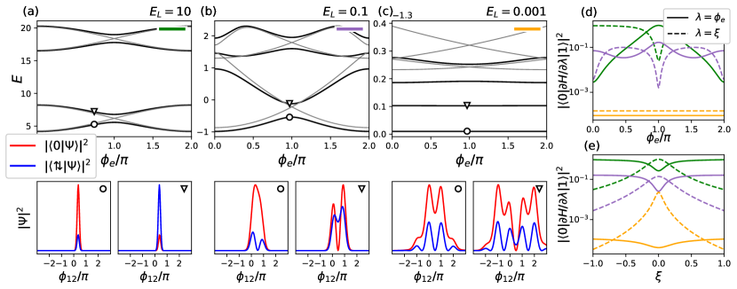
Figure 7: (a-c): Energy dispersion over the external phase $\phi_{e}$ for decreasing values of $E_{L}$ in the loop configuration with two leads, and wavefunctions indicated with markers (bottom panels – they are centered over $\phi_{12}\sim\phi_{e}/2$ because of the form of the inductive term $E_{L}(2\phi_{12}-\phi_{e})^{2}$). Grey lines indicate the resonant case with $E_{C_{12}}=1$, $\Gamma_{1,2}=1$ and $\xi=0$, and black lines indicate the case $\Gamma_{1}=0.95$, $\Gamma_{2}=1.05$ and $\xi=0.6$ (with a shift of $-\xi$). (d,e): Matrix elements associated to noise in $\phi_{e}$ and $\xi$ for the non-resonant parameters in a-c (setting $\phi_{e}=0.95\pi$ in e) and $\alpha{=}0$, indicating each case with the colours in the a-c corners.

We now consider the case where two leads are connected forming a loop (Fig. 1f), for which a different, more macroscopic model is required. We use the variable of tunneled pairs between the leads of the loop $\hat{N}_{12}{=}\hat{N}_{1}{-}\hat{N}_{2}$, conjugate to $\hat{\phi}_{12}$, with charging energy $E_{C_{12}}\hat{N}_{12}^{2}$. This model without the separate islands 1 and 2 is qualitatively different from the one derived in the previous section, because the loop disables the island nature of these leads, rendering the charge difference continuous [85] and allowing the presence of high energy persistent current states [127]. The charge in the remaining island $3$ remains discrete, and the total Hamiltonian is the combination $H_{12}+H_{3}+H_{d}+H_{c}$:

$$H_{12} =E_{C_{12}}\hat{N}_{12}^{2}+E_{L}(2\hat{\phi}_{12}-\phi_{e})^{2}$$

$$H_{3} =E_{C_{3}}(\hat{N}_{3}-n_{g_{3}})^{2}$$

$$H_{d} =\epsilon\sum_{\sigma}d^{\dagger}_{\sigma}d_{\sigma}+ud^{\dagger}_{\uparrow}d_{\uparrow}d^{\dagger}_{\downarrow}d_{\downarrow}$$

$$H_{c} =\left(\Gamma_{1}e^{-i\hat{\phi}_{12}}+\Gamma_{2}e^{i\hat{\phi}_{12}}+\Gamma_{3}e^{-i\hat{\phi}_{3}}\right)d^{\dagger}_{\uparrow}d^{\dagger}_{\uparrow}+h.c.\,,$$ (5)

where the Josephson processes that couple the dot with the leads in $H_{c}$ take into account that a tunneling of a pair from $\nu{=}1(2)$ to the dot level produces a shift in $N_{1}-N_{2}$ by $\mp 1$ (translation $e^{\mp i\hat{\phi}_{12}}$) and that a tunneling from $\nu=3$ to the dot level produces a change in $N_{3}$ (translation $e^{i\hat{\phi}_{3}}$). The Hamiltonian can be solved in the $\ket{\phi_{12},N_{3},n_{d}}$ basis with $\hat{N}_{12}=-i\partial_{\phi_{12}}$.

The phase drop $\phi_{e}=\Phi/\Phi_{0}$ is to be distributed among the inductance and the couplings $\Gamma_{1,2}$. In a dynamical situation, the correct description for a tunnel junction without Andreev structure corresponds to the phase dropping completely on the inductance [74, 76] (in absence of additional time dependent terms). However, in our case, a freedom in the drop distribution within the junction is still present ($\Gamma_{1,2}\rightarrow e^{if}\Gamma_{1,2}$ in $H_{c}$, Eq. (5)). We note that the inductive potential $E_{L}(2\hat{\phi}_{12}-\phi_{e})^{2}$ includes a factor of $2$ as the complete transfer of a pair from lead $1$ to lead $2$ requires two tunneling events. In the limit $L{\rightarrow}0$ ($E_{L}{\rightarrow}\infty$), the phase becomes localized at $\hat{\phi}_{12}{\rightarrow}\phi_{e}/2$, recovering the model in section II.

From a circuit perspective, the loop-island Hamiltonian contains two modes, one flux-like and one charge-like, which may be harnessed to devise protected qubits. These qubits would be similar in nature to the ones conceived in multimode circuits where several conventional elements generate the different modes [23]. In the remaining of this section, we explore the full Josephson-Andreev Hamiltonian, first in a one loop configuration, and then introducing a third floating lead. In section V, we focus on the cotunneling limit, which allows a straight-forward correspondence with the protected multi-element circuits.

IV.1 Two terminals forming one loop

This configuration is similar to a flux qubit when the Josephson-Andreev junction is in the tunneling regime [128, 129, 130, 131]. Otherwise, when the Andreev structure is close to resonance ($\Gamma_{1}{=}\Gamma_{2}$, $\xi{=}0$), it has been recently identified as a prospective protected qubit based on two disconnected states [21, 22].

In Fig. 7, we review the main features of the energy spectrum of this system, along with the corresponding wavefunctions. When $E_{L}$ is large compared with $E_{C}$ (Fig. 7a), the phase is localized and we recover the Andreev states of the central level from Section II. We note that the fermionic structure already provides a difference with the flux qubits, as the first excited level is an Andreev state. The associated wavefunctions (lower panels) are hybridizations between $\ket{0}$ and $\ket{\uparrow\downarrow}$ at a localized phase. In contrast, the excited states of the flux qubit are bosonic in nature, being harmonic oscillator-like wavefunctions with finite phase fluctuations enabled by the charging term, which acts as a kinetic energy in the phase representation. This kind of states correspond to Andreev replicas such as the higher doublet in Fig. 7a.

When $E_{L}$ is lowered, there is a competition between the inductive energy, a parabolic potential in phase representation, and the potential produced by the charge transfer terms. In the tunneling regime this potential is simply $-E_{J}\cos\hat{\phi}_{12}$, and the wavefunction may extend over two minima when $\phi_{e}=\pi$ and $E_{J}\sim E_{L}$, or several of the minima when $E_{L}\ll E_{J}$. In the latter case, if the kinetic energy $E_{C}$ is large compared to $E_{J}$, the wavefunction exceeds the maxima of the cosine and the phase delocalizes broadly; otherwise, the wavefunction localizes at several of the phase potential minima, and represents a superposition of discrete current states encircling the loop. In the junction with internal structure, the Andreev level introduces an additional degree of freedom. The limit $|\xi|\gg\Gamma$ recovers the previous tunneling regime where the states involve mainly just the lower energy Andreev state and the higher one is just virtually occupied to allow the flow of charge. However, in the resonant limit, both Andreev states participate. They are always degenerate at $\phi_{e}{=}\pi$ and if $E_{L}$ is lowered, their phase dependence decreases, providing a disjoint basis for a protected qubit insensitive to fluctuations in $\phi_{e}$ [21, 22]. The evolution with decreasing $E_{L}$ is shown in Fig. 7a,b,c where the black lines refer to a situation a bit out of resonance and the grey lines to a situation of full resonance, which maintain the Andreev degeneracy for any value of $E_{L}$.

In Fig. 7d,e we show the matrix elements $|\bra{0}\partial H/\partial\lambda\ket{1}|^{2}$ associated to noise in $\lambda{=}\phi_{e}$ ($\lambda{=}\xi$) between the two lowest energy states with solid (dashed) lines for the parameters in the panels a to c. There is a reduction in the matrix elements magnitude with the decrease of $E_{L}$ as the states spread over $\phi_{12}$ and become less sensitive to the Andreev degrees of freedom. In general, the protection against $\phi_{e}$ noise is enhanced when approaching resonance as the states share their structure in $\phi_{12}$ but are orthogonal in the Andreev sectors. On the contrary, the noise on the parameters $\xi,\delta\Gamma$ that move away from resonance is more harmful in that regime as it produces dephasing due to the linear splitting of the energy levels. Finally, there is the issue of the phase drop distribution. In Fig. 7d,e we have used a symmetric drop in the couplings with the central level ($\alpha=0$), as expected in an homogeneous field situation with almost symmetric coupling strengths $\Gamma_{1,2}$. However, a finite $\alpha$ would boost the effect of the $\phi_{e}$ noise because the pair tunneling terms would start to contribute to $\partial H/\partial\phi_{e}$.

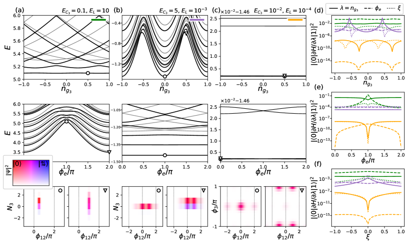
Figure 8: (a-c): Energy dispersion over the charge offset $n_{g_{3}}$ (top panels) and the external phase $\phi_{e}$ (middle panels) in the loop configuration where a third terminal is a charge island, and wavefunctions indicated with markers (bottom panels – the coloured inset is a legend that represents the participation of the central level in the wavefunction). Grey lines indicate the resonant case and black ones a situation a bit out of resonance. In panel (a), the island is in the transmon regime (delocalized $\hat{N}_{3}$) and the loop is close to a phase biased regime (well localized phase, parameters of Fig. 7a and $\Gamma_{3}{=}1$). In panel (b), the island is in the Cooper pair box regime (localized $\hat{N}_{3}$, with only two states participating in the global wavefunctions), and the loop in a fluxonium regime (delocalized phase, parameters of Fig. 7b and $\Gamma_{3}{=}1$). This is similar to a bifluxon. In panel (c), the island has delocalized charge and loop has delocalized phase (the resonant condition has a similar spectrum and it is not shown). This is similar to a 0-$\pi$ qubit – the wavefunction is displayed in the $\ket{\phi_{12},\phi_{3}}$ basis to show that the wavefunctions of the two lowest states are disjoint. Parameters: $E_{C_{12}}{=}1$, $\Gamma_{1}{=}0.4$, $\Gamma_{2}{=}0.6$, $\Gamma_{3}{=}1$ and $\xi{=}0.6$. (d-f): Matrix elements associated to noise in $n_{g_{3}}$, $\phi_{e}$ and $\xi$ for the non-resonant parameters in (a-c) in the circle markers, and indicating each case with the colours in the (a-c) corners.

IV.2 Three terminals: one loop and one island

In the previous subsection we have seen that a low inductive potential favours the insensitivity to dephasing produced by $\phi_{e}$ noise. However, in order to achieve the protection against decoherence it is necessary to have two states which are disjoint over a different degree of freedom, such that $\partial H/\partial\phi_{e}$ does not connect them. These two states were provided by the fermionic structure of the junction in the resonant limit, which fulfils this purpose but introduces new sources of noise [21, 22]. We explore now the situation where a third terminal with charging energy is introduced (Eq. (5)), and how it can provide disjoint states of a different origin.

We begin in Fig. 8a by connecting the loop with two terminals in the phase localized regime of Fig. 7a to an island in the transmon regime (delocalized charge). In the phase biased limit we have $E_{L}{\rightarrow}\infty$, $\hat{\phi}_{12}{\rightarrow}\phi_{e}/2$ and the configuration is similar to the one in Sec. III.2, where the central region is connected to one charge island and to one terminal without charging energy. In this analogy, $\Gamma_{3}$ is the coupling that shifts the occupation number of the island, and the term $\Gamma_{12}(\phi_{e})=\Gamma_{1}e^{-i\phi_{e}/2}+\Gamma_{2}e^{i\phi_{e}/2}$ is the coupling that connects the central level states at a fixed island occupation, which is now tunable by $\phi_{e}$. This arrangement connects all sites in the resulting $\ket{N_{3},n_{d}}$ chain and, as a result, the occupation of the island is determined by the combination of all the couplings, not only $\Gamma_{3}$. For instance, the wavefunction marked with a circle in Fig. 8a has a lower charge dispersion that the one with a triangle because at $\phi_{e}=\pi$ the effective coupling $\Gamma_{12}(\phi_{e})$ is reduced.

In Fig. 8b we combine the phase extended regime of Fig. 7c in the loop with the island in the Cooper pair box limit (strongly localized charge, thus, it can be described with the two number states of lower energy). This situation benefits of the $\phi_{e}$ insensitivity already discussed in the previous subsection, but now the central region and the island hybridize into essentially $4$ levels. The phase potential they generate can produce disjoint states in the limit where only one level in the island (central region) contributes, and thus the central region (island) may be set at resonance. The first case is similar to the configuration of the previous subsection, and the second one describes the tunneling regime in the central region while two island states play the role of an effective resonant dot (discussed in next section and in Appendix D). The protection of this configuration is analogous to that of a bifluxon qubit [32].

In Fig. 8c, we set the protected regime in each degree of freedom. The wavefunctions are delocalized over $\hat{\phi}_{12}$ and $\hat{N}_{3}$ (fluxonium and transmon-like), producing flat transition energies over the parameters $n_{g_{3}}$ and $\phi_{e}$, so the qubit states are protected against dephasing by the associated charge and flux noise. The protection against relaxation occurs because the states have disjoint wavefunctions (see lower panels for the wavefunctions and panels d to f for the matrix elements associated to noise on $n_{g_{3}}$, $\phi_{e}$ and $\xi$ for the settings in panels a to c). This disjointness is only observed in the space $\ket{\phi_{12},\phi_{3}}$, but the fact that the wavefunctions overlap in the space $\ket{\phi_{12},N_{3}}$ does not mean that it is not protected against noise on $n_{g_{3}}$, as the associated operator $\hat{N}_{3}=-i\partial_{\phi_{3}}$ is local in the phase coordinate. The same applies to a possible charge noise in the loop with $\hat{N}_{12}\rightarrow\hat{N}_{12}{-}n_{g_{12}}$. Thus, the protection of this configuration is analogous to that of a $0-\pi$ qubit [31]. This and the previous connection with protected qubits designed in multimode circuits made out from several traditional elements will be more easily discussed in the next section when focusing on the tunneling regime.

V Cotunneling limit

At certain limits, a non-tunnel Josephson junction embedded in a circuit can be described as a lumped element, i.e., an effective tunnel junction (Fig. 1c, Sec. III.2 and Appendix B), which is characterized by the phase dispersion of the lowest energy Andreev state. This adiabatic approximation in a multiterminal situation provides an interpretation in terms of processes that distribute pairs between the leads, i.e. a combination of lumped junctions between each terminal. For example, in a 3-terminal configuration with time reversal symmetry (e.g. in Fig. 2), the ground state can be written as

$$E_{0}(\phi_{1},\phi_{2})=\sum_{n_{1},n_{2}\in\mathbb{Z}}A_{n_{1},n_{2}}\cos\left(n_{1}\phi_{1}{+}n_{2}\phi_{2}\right),$$

where the form ${\propto}\cos\left(n_{1}\phi_{1}{+}n_{2}\phi_{2}\right)$ can be associated to processes where several Cooper pairs from one lead split into the other two. This association may be done by defining the phase variables in correspondence with their operator counterparts in Sec. III. There, by using the reduced basis $\ket{N_{1},N_{2}}$, a tunneling from terminals $1\rightarrow 3$ ($2\rightarrow 3$) is produced by the traslation operator $e^{-i\hat{\phi}_{1}}$ ($e^{-i\hat{\phi}_{2}}$), and from $1\rightarrow 2$ by $e^{-i\hat{\phi}_{1}+i\hat{\phi}_{2}}$. In this way, the phase variables recover their operator nature conjugate to charge-like variables in the resulting effective Hamiltonian $H^{\textrm{eff}}_{J}(\hat{\phi}_{1},\hat{\phi}_{2})$ .

In particular, if we only consider single pair tunneling processes, the effective tunneling Hamiltonian is

$$H^{\textrm{eff}}_{J}=-E_{J_{13}}\cos\hat{\phi}_{1}-E_{J_{23}}\cos\hat{\phi}_{2}-E_{J_{12}}\cos{(\hat{\phi}_{1}{-}\hat{\phi}_{2})},$$

with $E_{J_{13}}{=}A_{1,0}$, $E_{J_{23}}{=}A_{0,1}$ and $E_{J_{12}}{=}A_{1,-1}$. We use this case to analyse the following limits.

Trijunction in an island configuration

In the harmonic limit of an island configuration (all $E_{C}\ll$ all $E_{J}$), the wavefunctions localize in phase so we can approximate $H_{J}^{\textrm{eff}}\approx(E_{J_{13}}+E_{J_{12}})\hat{\phi}_{1}^{2}/2+(E_{J_{23}}+E_{J_{12}})\hat{\phi}_{2}^{2}/2-E_{J_{12}}\hat{\phi}_{1}\hat{\phi}_{2}$. The charge offsets $n_{g}$ have no effect in this limit (the charge becomes continuous and the $n_{g}$ a gauge freedom [85]) and we can write $H^{\textrm{eff}}_{\textrm{harm}}=\vec{N}^{T}\mathbb{C}\vec{N}+\vec{\phi}^{T}\mathbb{J}\vec{\phi}$ where $\vec{N}=(\hat{N}_{1},\hat{N}_{2})^{T}$, $\vec{\phi}=(\hat{\phi}_{1},\hat{\phi}_{2})^{T}$ and

$$\mathbb{C}{=}\begin{pmatrix}E_{C_{1}}{+}E_{C_{3}}&E_{C_{3}}\\ E_{C_{3}}&E_{C_{2}}{+}E_{C_{3}}\end{pmatrix}, \mathbb{J}{=}\frac{1}{2}\begin{pmatrix}E_{J_{13}}{+}E_{J_{12}}&{-}E_{J_{12}}\\ {-}E_{J_{12}}&E_{J_{23}}{+}E_{J_{12}}\end{pmatrix},$$ (6)

such that the Hamiltonian can be diagonalized into two harmonic modes $H^{\textrm{eff}}_{\textrm{harm}}=\sum_{\nu}\omega_{\nu}(a^{\dagger}_{\nu}a_{\nu}+1/2)$ (see details and extensions provided in Appendix C).

In the limit where one island is in a Cooper pair box regime (e.g. $E_{C_{3}}\gg E_{J_{13}},E_{J_{23}}$), that island can be described with a two level model, one for each of the lowest energy number $N_{3}$ occupations. As elaborated in Appendix D, it maps to the model of the Josephson-Andreev junction with two terminals in Sec. III when $E_{J_{12}}=0$ (the terminal $3$ would play the role of the central level).

Trijunction with two terminals in a loop
and one island configuration

If two terminals close themselves forming a loop, the model is similar to the one in Sec. IV, where the variables are the tunneled pairs between the leads of the loop $\hat{N}_{12}$ and the number of pairs $\hat{N}_{3}$ in the island. The effective Hamiltonian is $H_{12}+H_{3}+H_{c}$, where

$$H_{12}=E_{C_{12}}\hat{N}_{12}^{2}+E_{J_{12}}\cos 2\hat{\phi}_{12}+E_{L}(2\hat{\phi}_{12}-\phi_{e})^{2}$$

$$H_{3}=E_{C_{3}}(\hat{N}_{3}-n_{g_{3}})^{2}$$

$$H_{c}=E_{J_{13}}\cos{(\hat{\phi}_{12}+\hat{\phi}_{3})}+E_{J_{23}}\cos{(\hat{\phi}_{12}-\hat{\phi}_{3})}\,,$$ (7)

and the operator $e^{i2\hat{\phi}_{12}}$ transfers a pair from $1\rightarrow 2$, $e^{i\hat{\phi}_{12}+i\hat{\phi}_{3}}$ from $1\rightarrow 3$ and $e^{i\hat{\phi}_{12}-i\hat{\phi}_{3}}$ from $2\rightarrow 3$. The Hamiltonian can be solved in the basis $\ket{\phi_{12},N_{3}}$, and contains two modes which can be harnessed to devise protected qubits similarly to multimode circuits designed with SIS tunnel junctions [23]. Two conventional limits are the following.

On the one hand, if $E_{J_{12}}\gg E_{J_{13}},\,E_{J_{23}}$, the Hamiltonian is similar to a “$\cos 2\varphi$” qubit as the potential in $\hat{\phi}_{12}$ is almost $\pi$ periodic [35, 38]. Physically, the situation with only $E_{J_{12}}$ tunneling conserves the parity of tunneled pairs, generating two disconnected sets of states.

On the other hand, if $E_{J_{12}}=0$ and $E_{J_{13}}=E_{J_{23}}:=E_{J}^{\prime}$, the coupling becomes

$$H_{c}=E_{J}^{\prime}\cos{\hat{\phi}_{12}}\cos{\hat{\phi}_{3}},$$

recovering the typical expression for multimode circuits, such as the bifluxon or the $0{-}\pi$ qubit, at the corresponding parameter regime [23].

VI Conclusions

Mesoscopic Josephson junctions host localized states with phase-dependent energy which can be probed in spectroscopy and manipulated coherently using microwave pulses. The number of these states, their spin texture and their energy are sensitive to internal as well as control parameters such as electric fields applied with a gate voltage, magnetic fields or strain. Compared to standard tunnel junctions, the energy of the fermionic excitations may become of the same order as the collective bosonic modes of quantum circuits that include capacitors and inductors. This “mesoscopic embbeding” constitutes a promising experimental and theoretical research topic with opportunities to develop hybrid fermionic-bosonic devices more immune to decoherence and relaxation than conventional ones. Additionally, on a fundamental level, these devices raise questions on the proper modelling and on the correct quantum circuit rules for their combination. In this work we have addressed these questions taking a three-terminal junction connected in different configurations as a model system.

While exploring the energy spectrum and the wavefunctions of these Josephson-Andreev junctions for different circuit configurations we have identified regimes of charge and/or flux noise protection against dephasing and/or relaxation. We have discussed different limiting cases for each configuration to recover known results, and for the multiterminal configurations we have shown their connection with other kinds of protected qubits such as the bifluxon or the $0{-}\pi$ qubits obtained using standard tunnel junctions arrays. This fact highlights how the multi-mode character of these circuits can be emulated thanks to the connectivity of the multiterminal ones, with the additional value of their higher degree of tunability.

Regarding the modelling, the nuance of the gauge choice for time dependent situations, which includes the considerations about the noise, emerges as an important issue to care about. Though we provide some orientation for this choice in our problem, its strong effect suggests that experimental guidance would be required for more conclusive estimations. Additionally, several open issues remain to be investigated, such as the robustness with respect to quasiparticle poisoning, which requires a more elaborate model for the superconducting leads, or the design of suitable operation protocols. We expect that the present work could motivate further experimental and theoretical efforts along these lines of research.

Appendix A Effective Hamiltonian
in phase biased conditions

Our starting point is a single-level model coupled to superconducting leads, described by a Hamiltonian of the form

$$H=\sum_{\sigma}\epsilon d^{\dagger}_{\sigma}d_{\sigma}+H_{T}+\sum_{\nu}H_{\nu}\;,$$

where $H_{\nu}$ correspond to the different terminals ($\nu$ ranging from 1 to 3 in the trijunction case) and

$$H_{T}=\sum_{\nu,\sigma,k}t_{\nu}e^{-i\phi_{\nu}/2}d^{\dagger}_{\sigma}c_{\nu,k\sigma}+\mbox{h.c.}$$

where $\phi_{\nu}$ is the superconducting phase on each lead.

Using conventional field theoretical methods one can integrate out the leads, leading to an effective action on the dot

$$S_{\text{eff}}=\int dtdt^{\prime}\bar{\psi}_{d}(t)\left[i\delta(t-t^{\prime})\left(\partial_{t}-\epsilon\tau_{z}\right)-\hat{\Sigma}(t,t^{\prime})\right]\psi_{d}(t^{\prime})\;$$ (8)

where $\psi_{d}$ is the Grassman field associated with the dot Nambu spinor $(d_{\uparrow}\;d^{\dagger}_{\downarrow})^{T}$, and $\hat{\Sigma}(t,t^{\prime})$ denotes the leads self-energy given by

$$\hat{\Sigma}(t,t^{\prime})=\sum_{\nu}t^{2}_{\nu}e^{-i\phi_{\nu}(t)\tau_{z}/2}\hat{g}(t-t^{\prime})e^{i\phi_{\nu}(t^{\prime})\tau_{z}/2}\;.$$

For the uncoupled leads Green functions $\hat{g}(t-t^{\prime})$ we can use the BCS model in the wide band approximation, i.e.

$$\hat{g}(t-t^{\prime})=\int\frac{d\omega}{2\pi}e^{i\omega(t-t^{\prime})}\left[\frac{-\omega\tau_{0}+\Delta\tau_{x}}{W\sqrt{\Delta^{2}-\omega^{2}}}\right]\;,$$

where $W$ denotes the bandwidth. In the static case and in the absence of phase fluctuations (constant $\phi_{\nu}$) Eq. 8 can be written as

$$S_{\text{eff}}=\int d\omega\bar{\psi}_{d}(\omega)\Biggl{[}\omega-\epsilon\tau_{z}-\\ \left.\sum_{\nu}\Gamma_{\nu}\left(\frac{-\omega\tau_{0}+\Delta\left(\tau_{x}\cos\phi_{\nu}-\tau_{y}\sin\phi_{\nu}\right)}{\sqrt{\Delta^{2}-\omega^{2}}}\right)\right]\psi_{d}(\omega)\;,$$

where $\Gamma_{\nu}=t^{2}_{\nu}/W$. In the large gap limit, i.e. $\omega\ll\Delta$ the model is characterized by bound states at

$$E_{A}(\left\{\phi_{\nu}\right\})=\sqrt{\epsilon^{2}+|\sum_{\nu}\Gamma_{\nu}e^{-i\phi_{\nu}}|^{2}}\,.$$

On the other hand, in the presence of phase fluctuations Eq. 8 can be simplified following the lines of [79]. For that purpose we approximate $\hat{g}(t-t^{\prime})$ as

$$\hat{g}(t-t^{\prime})\simeq\delta(t-t^{\prime})\frac{-i\partial_{t}\tau_{0}+\Delta\tau_{x}}{W\Delta}\;,$$

which leads to

$$S_{\text{eff}}=\int dt\bar{\psi}_{d}(t)\Biggl{[}i\partial_{t}-\epsilon\tau_{z}-\\ \left.\sum_{\nu}\Gamma_{\nu}\left(\tau_{x}\cos\phi_{\nu}(t)-\tau_{y}\sin\phi_{\nu}(t)-\tau_{z}\frac{\dot{\phi}_{\nu}(t)}{2\Delta}\right)\right]\psi_{d}(t)\;.$$

To remove the $\dot{\phi}_{\nu}$ terms we redefine $\psi_{d}(t)\rightarrow e^{-i\sum_{\nu}\tilde{\Gamma}_{\nu}\phi_{\nu}\sigma_{z}}\psi_{d}(t)$, where $\tilde{\Gamma}_{\nu}=\frac{\Gamma_{\nu}}{2\Delta}$, so that

$$S_{\text{eff}}=\int dt\bar{\psi}_{d}(t)\left[i\partial_{t}-\hat{H}_{\text{eff}}\right]\psi_{d}(t)\;,$$

where

$$\hat{H}_{\text{eff}}=e^{-i\sum_{\nu}\tilde{\Gamma}_{\nu}\phi_{\nu}\tau_{z}}\Biggl{[}\epsilon\tau_{z}+\\ \left.\sum_{\nu}\Gamma_{\nu}\left(\tau_{x}\cos\phi_{\nu}-\tau_{y}\sin\phi_{\nu}\right)\right]e^{i\sum_{\nu}\tilde{\Gamma}_{\nu}\phi_{\nu}\tau_{z}}\;.$$ (9)

This last expression can be used as the effective Hamiltonian for the multi-terminal quantum dot junction. In practice only two out of the three phases $\left\{\phi_{\nu}\right\}$ can be considered independent. In particular, in the infinite gap limit one can disregard the phase prefactors in Eq. 9.

Appendix B Adiabatic approximation

When transforming from the number space to the phase space (for simplicity in a 2-terminal configuration with one degree of freedom), it is convenient to interpret the latter as a discrete grid, that arises when the number space is truncated to an arbitrarily large interval $N{\in}[-N^{M},N^{M}]$ with periodic boundary conditions, defining $\ket{\phi_{n}}=N_{\#}^{-1/2}\sum_{N}e^{iN\phi_{n}}\ket{N}$, with $N_{\#}=2N^{M}{+}1$ and $\phi_{n}{=}2\pi n/N_{\#}$. This is justified because at finite charging energy the wavefunction has no infinite extension in $N$. Then, the operator $\hat{N}$ can be thought as a translation in the $\ket{\phi_{n}}$’s, with $\hat{N}^{2}\approx 2N_{\#}^{2}(1-\cos\hat{N}/N_{\#})$. In the continuum limit this converts into the second derivative ${-}\partial_{\phi}^{2}$.

At each point $\phi$, the potential Hamiltonian $H_{A}(\phi)$ is equivalent to the one describing the phase biased configuration (Eq. 2), up to a gauge transformation. The Andreev transformation $U(\phi)H_{A}(\phi)U^{\dagger}(\phi)=\mathbb{E}_{A}$ diagonalizes the states at each phase point, but then the kinetic term $\sim E_{C}\hat{N}^{2}$ becomes non-diagonal in the neighbouring phase hoppings:

$$\hat{N}^{2}\rightarrow\hat{N}^{2}-i\anticommutator{U(\phi)U^{\prime\dagger}(\phi)}{\hat{N}}-(U(\phi)U^{\prime\dagger}(\phi))^{2},$$

where $U^{\prime}(\phi)=\partial_{\phi}U(\phi)$, and it has been used that $\partial_{\phi}(U(\phi)U^{\dagger}(\phi))=0$. The adiabatic approximation consists in truncating the Andreev sector to its ground state (with energy equal to $\min{\{\mathbb{E}_{A}\}}$) and keeping the main kinetic term, which is the one with $\hat{N}^{2}$ since in the transmon-like regime the wavefunction is strongly delocalized in charge. We note that the Andreev transformation has distorted the number translation and that there is a gauge dependence similar to the one in Sec. II, that arises from the choice of the reduced number basis (the complete charging term would also depend on it). When restricted to the truncated Andreev sector, it has a similar role to a phase dependent charge offset and a phase potential, which becomes less noticeable as the charge delocalizes.

In this limit, the phase localizes and we can expand the effective potential into an anharmonic oscillator

$$H^{\textrm{eff}}_{\text{osc}}=E_{C}\hat{N}^{2}+E^{\textrm{eff}_{2}}_{J}\hat{\phi}^{2}+E^{\textrm{eff}_{4}}_{J}\hat{\phi}^{4},$$

with $E_{J}^{\textrm{eff}_{n}}=\partial^{n}_{\phi}E_{0}(\phi)\bigr{\rvert}_{\phi{=}0}/n!$, which in the harmonic basis $\ket{m}{=}(a^{\dagger})^{m}\ket{0}/\sqrt{m!}$, with $a^{(\dagger)}=(E_{J}^{\textrm{eff}_{2}}/4E_{C})^{1/4}\hat{\phi}_{1}\mp i(E_{C}/4E_{J}^{\textrm{eff}_{2}})^{1/4}\hat{N}$ (see Appendix C), produces states with energies $E_{m}$

$$2\sqrt{E_{C}E_{J}^{\textrm{eff}_{2}}}\left(m+1/2\right)+\frac{E_{C}E_{J}^{\textrm{eff}_{4}}}{4E_{J}^{\textrm{eff}_{2}}}\left(6m^{2}+6m+3\right),$$

up to $\textrm{1}^{\textrm{st}}$ order perturbation theory. This yields a transition $E_{01}$ equal to the prefactors on $m$ (the one with the square root is referred with $\omega$ in the main text) and an anharmonicity $\alpha_{h}:=E_{12}{-}E_{01}$ equal to twice the prefactors on $m^{2}$. Within the model of Sec. II, $E_{J}^{\textrm{eff}_{2}}=(\Gamma^{2}{-}\delta\Gamma^{2})/8\sqrt{\Gamma^{2}{+}\xi^{2}}$ and $\alpha=E_{C}\left({-}1/4+3(\Gamma^{2}{-}\delta\Gamma^{2})/16(\Gamma^{2}{+}\xi^{2})\right)$.

Appendix C Simultaneous diagonalization
in the tunnel limit

The matrix $\mathbb{C}$ in Eq. 6 is positive definite, hence it can be written [132]

$$\mathbb{C}=(v_{C})D_{C}(v_{C})^{T}=\left[(v_{C})\sqrt{D_{C}}\right]\left[(v_{C})\sqrt{D_{C}}\right]^{T}:=R^{T}R,$$ (10)

where $v_{C}$ is the matrix made of the orthonormal vectors that diagonalize $\mathbb{C}$ into $D_{C}$. Note that if we define $C_{N}{=}R^{-1}U$, with any unitary $U^{T}{=}U^{-1}$, we have $C_{N}^{T}\mathbb{C}C_{N}=\mathbbm{1}$. Now, consider that there is $C_{\phi}$ such that $C_{\phi}^{T}\mathbb{J}C_{\phi}=D_{J}$ with diagonal $D_{J}$, and that $C_{\phi}^{T}=C_{N}^{-1}$ for reasons that will be clear afterwards – it is allowed because in a Hamiltonian formulation the conjugate variables are independent [133]. Then the previous equation for $D_{J}$ can be written as the diagonalization $U^{T}(R\mathbb{J}R^{T})U=D_{J}\leftrightarrow R\mathbb{J}R^{T}U=UD_{J}$, showing that $U=(u_{1},u_{2},...)$ is made of the eigenvectors from that diagonalization, which is possible because the matrix product between parenthesis is symmetric. Multiplying by $R^{-1}$ it is equivalent to

$$\mathbb{J}R^{T}U=R^{-1}UD_{J}=R^{-1}R^{-1T}VD_{J}=\mathbb{C}VD_{J},$$ (11)

where $V:=R^{T}U$ shows the structure of a generalized diagonalization into the columns of $V=(v_{1},v_{2},...)$, with eigenvalues $\lambda$ satisfying $\textrm{det}(\mathbb{J}-\mathbb{C}\lambda)=0$. Note that $v_{n}^{T}\mathbb{C}^{-1}v_{m}=v_{n}^{T}R^{-1}R^{-1T}v_{m}=u_{n}^{T}u_{m}=\delta_{nm}$.

Then we can write $H^{\textrm{eff}}_{\textrm{harm}}{=}\vec{N}^{\prime T}\vec{N}^{\prime}{+}\vec{\phi}^{\prime T}D_{J}\vec{\phi}^{\prime}$, with $\vec{N}^{\prime}{=}C_{N}^{-1}\vec{N}$ and $\vec{\phi}^{\prime}{=}C_{\phi}^{-1}\vec{\phi}$. Each transformed pair $(\hat{N}^{\prime}_{\nu},\hat{\phi}^{\prime}_{\nu})$ is uncoupled from the others, and we have $\commutator{\hat{\phi}^{\prime}_{\mu}}{\hat{\phi}^{\prime}_{\nu}}{=}0$, $\commutator{\hat{N}^{\prime}_{\mu}}{\hat{N}^{\prime}_{\nu}}{=}0$ and $\commutator{\hat{\phi}^{\prime}_{\mu}}{\hat{N}^{\prime}_{\nu}}{=}i\sum_{\alpha}(C^{-1}_{\phi})_{\mu\alpha}(C^{-1}_{N})_{\nu\alpha}{=}i(C^{-1}_{\phi}C^{-1T}_{N})_{\mu\nu}{=}i\delta_{\mu\nu}$, where the choice in the previous paragraph allows to conserve the commuting properties in the transformed operators.

Now, defining $a_{\nu}^{(\dagger)}=c_{1\nu}^{(*)}\hat{N}^{\prime}_{\nu}+c_{2\nu}^{(*)}\hat{\phi}^{\prime}_{\nu}$, the commutation relations $\commutator{a_{\mu}}{a_{\nu}^{\dagger}}=\delta_{\mu\nu}$ constrain $c_{1\nu}c_{2\nu}{=}{-}1/2$. Then, $H^{\textrm{eff}}_{\textrm{harm}}$ can be made diagonal with the choice $c_{1,2\nu}{=}(D_{J})_{\nu}^{\pm 1/4}i^{-1/2\pm 1/2}/\sqrt{2}$. Finally, $H^{\textrm{eff}}_{\textrm{harm}}=\sum_{\nu}2\sqrt{D_{J_{\nu}}}(a^{\dagger}_{\nu}a_{\nu}+1/2)$, where $(D_{J})_{\nu}=\left(b\pm\sqrt{b^{2}-4c}\right)/4$, with

$$b=\sum_{\alpha=1}^{3}E_{C_{\alpha}}\left(E_{J_{\alpha,\alpha-1}}+E_{J_{\alpha,\alpha+1}}\right)$$

$$c=\left(\sum_{\alpha=1}^{3}E_{C_{\alpha}}E_{C_{\alpha+1}}\right)\left(\sum_{\alpha=1}^{3}E_{J_{\alpha-1,\alpha}}E_{J_{\alpha,\alpha+1}}\right),$$

where the indexes values $0$ and $4$ refer to the indexes $3$ and $1$, respectively, and $E_{J_{\mu\nu}}{=}E_{J_{\nu\mu}}$. Some particular cases are $2D_{J_{\nu}}{=}\{0,\,(E_{C_{1}}{+}E_{C_{2}})E_{J_{12}}\}$ for $E_{J_{13}}{=}0{=}E_{J_{23}}$, and $2D_{J_{\nu}}{=}\{E_{C_{1}}E_{J_{13}},\,E_{C_{2}}E_{J_{23}}\}$ for $E_{J_{12}}{=}0{=}E_{C_{3}}$.

Appendix D Two level island limit

In the limit $E_{C_{3}}\gg E_{J_{13}},E_{J_{23}}$, we can describe island $3$ with its two lowest energy levels corresponding to certain $N_{3}$ and $N_{3}+1$, with an energy difference of $2(n_{g3}-1/2)$. In this case it is useful to describe the other two terminals with $\hat{N}_{12}=\hat{N}_{1}-\hat{N}_{2}$ (note that a third variable is not necessary - the charge conservation imposes the value of the remaining $\hat{N}_{1}+\hat{N}_{2}$). The tunneling processes between $1$ and $2$ create an imbalance of $2$ pairs in $N_{12}$ ($-E_{J_{12}}e^{-i2\hat{\phi}_{12}}+h.c.$), while the tunneling from $1$ to the island and from the island to $3$ creates an imbalance of $1$ pair ($-E_{J_{13}}e^{-i\hat{\phi}_{12}}\ket{N_{3}+1}\bra{N_{3}}+h.c.$ and $-E_{J_{23}}e^{-i\hat{\phi}_{12}}\ket{N_{3}}\bra{N_{3}+1}+h.c.$, respectively). Thus, in the basis $\{\ket{N_{3}},\,\ket{N_{3}+1}\}$,

$$H^{\textrm{eff}}_{\textrm{2lvs}}=H_{C}-E_{J_{12}}\cos{2\hat{\phi}_{12}}\,+\\ \begin{pmatrix}-(n_{g_{3}}-1/2)&-E_{J_{13}}e^{i\hat{\phi}_{12}}-E_{J_{23}}e^{-i\hat{\phi}_{12}}\\ -E_{J_{13}}e^{-i\hat{\phi}_{12}}-E_{J_{23}}e^{i\hat{\phi}_{12}}&n_{g_{3}}-1/2\end{pmatrix},$$ (12)

where the correspondence with the 2-terminals junction with a central level is given by $\xi=n_{g_{3}}{-}1/2$ and $\Gamma_{1,2}=-E_{J_{13,23}}$ (at $E_{J_{12}}{=}0$). From a different perspective, in the case of $E_{J_{12}}\gg E_{C_{12}}$, this tunneling term can be diagonalized with the charging term into an oscillator coupled to the 2-level structure. This is similar to what occurs when coupling a circuit with a reference transmon [104].

References

- Clarke et al. [1988] J. Clarke, A. N. Cleland, M. H. Devoret, D. Esteve, and J. M. Martinis, Quantum Mechanics of a Macroscopic Variable: The Phase Difference of a Josephson Junction, Science 239, 992 (1988).
- Blais et al. [2021] A. Blais, A. L. Grimsmo, S. M. Girvin, and A. Wallraff, Circuit quantum electrodynamics, Rev. Mod. Phys. 93, 025005 (2021).
- Nazarov and Blanter [2009] Y. V. Nazarov and Y. M. Blanter, Quantum Transport: Introduction to Nanoscience (Cambridge University Press, 2009).
- Kulik [1969] I. O. Kulik, Macroscopic quantization and the proximity effect in S-N-S junctions, Pis’ma Zh. Eksp. Teor. Fiz [ [Sov. Phys. JETP 30, 944 (1970)] 57 (1969).
- Furusaki et al. [1991] A. Furusaki, H. Takayanagi, and M. Tsukada, Theory of quantum conduction of supercurrent through a constriction, Physical Review Letters 67, 132 (1991).
- Beenakker and van Houten [1991] C. W. J. Beenakker and H. van Houten, Josephson current through a superconducting quantum point contact shorter than the coherence length, Physical Review Letters 66, 3056 (1991).
- Bargerbos et al. [2020] A. Bargerbos, W. Uilhoorn, C.-K. Yang, P. Krogstrup, L. P. Kouwenhoven, G. de Lange, B. van Heck, and A. Kou, Observation of Vanishing Charge Dispersion of a Nearly Open Superconducting Island, Phys. Rev. Lett. 124, 246802 (2020).
- Pita-Vidal et al. [2022] M. Pita-Vidal, A. Bargerbos, R. Žitko, L. J. Splitthoff, L. Grünhaupt, J. J. Wesdorp, Y. Liu, L. P. Kouwenhoven, R. Aguado, B. van Heck, A. Kou, and C. K. Andersen, Direct manipulation of a superconducting spin qubit strongly coupled to a transmon qubit (2022).
- Kringhøj et al. [2018] A. Kringhøj, L. Casparis, M. Hell, T. W. Larsen, F. Kuemmeth, M. Leijnse, K. Flensberg, P. Krogstrup, J. Nygård, K. D. Petersson, and C. M. Marcus, Anharmonicity of a superconducting qubit with a few-mode Josephson junction, Phys. Rev. B 97, 060508 (2018).
- Kringhøj et al. [2020] A. Kringhøj, B. van Heck, T. W. Larsen, O. Erlandsson, D. Sabonis, P. Krogstrup, L. Casparis, K. D. Petersson, and C. M. Marcus, Suppressed Charge Dispersion via Resonant Tunneling in a Single-Channel Transmon, Phys. Rev. Lett. 124, 246803 (2020).
- Coraiola et al. [2023a] M. Coraiola, D. Z. Haxell, D. Sabonis, M. Hinderling, S. C. t. Kate, E. Cheah, F. Krizek, R. Schott, W. Wegscheider, and F. Nichele, Spin-degeneracy breaking and parity transitions in three-terminal Josephson junctions (2023a).
- Fu [2010] L. Fu, Electron Teleportation via Majorana Bound States in a Mesoscopic Superconductor, Physical Review Letters 104, 10.1103/physrevlett.104.056402 (2010).
- van Heck et al. [2011] B. van Heck, F. Hassler, A. R. Akhmerov, and C. W. J. Beenakker, Coulomb stability of the 4-periodic Josephson effect of Majorana fermions, Physical Review B 84, 10.1103/physrevb.84.180502 (2011).
- Karki et al. [2023] D. B. Karki, K. A. Matveev, and I. Martin, Physics of the Majorana-superconducting qubit hybrids (2023).
- Keselman et al. [2019] A. Keselman, C. Murthy, B. van Heck, and B. Bauer, Spectral response of Josephson junctions with low-energy quasiparticles, SciPost Physics 7, 10.21468/scipostphys.7.4.050 (2019).
- Ávila et al. [2020] J. Ávila, E. Prada, P. San-Jose, and R. Aguado, Superconducting islands with topological Josephson junctions based on semiconductor nanowires, Physical Review B 102, 10.1103/physrevb.102.094518 (2020).
- Ávila et al. [2020] J. Ávila, E. Prada, P. San-Jose, and R. Aguado, Majorana oscillations and parity crossings in semiconductor nanowire-based transmon qubits, Phys. Rev. Res. 2, 033493 (2020).
- Pino et al. [2023] D. M. Pino, R. S. Souto, and R. Aguado, Minimal Kitaev-transmon qubit based on double quantum dots (2023).
- Bretheau et al. [2014] L. Bretheau, Ç. O. Girit, M. Houzet, H. Pothier, D. Esteve, and C. Urbina, Theory of microwave spectroscopy of Andreev bound states with a Josephson junction, Phys. Rev. B 90, 134506 (2014).
- Vakhtel and van Heck [2023] T. Vakhtel and B. van Heck, Quantum phase slips in a resonant Josephson junction, Phys. Rev. B 107, 195405 (2023).
- Caceres [2022] J. J. Caceres, Qubit protegido contra errores y compuertas cuánticas rápidas basadas en la transición Landau-Zener-Stuckelberg, Master’s thesis, Centro Atómico Bariloche, Instituto Balseiro (2022).
- Vakhtel et al. [2023] T. Vakhtel, P. D. Kurilovich, M. Pita-Vidal, A. Bargerbos, V. Fatemi, and B. van Heck, Tunneling of fluxons via a Josephson resonant level (2023).
- Gyenis et al. [2021a] A. Gyenis, A. Di Paolo, J. Koch, A. Blais, A. A. Houck, and D. I. Schuster, Moving beyond the Transmon: Noise-Protected Superconducting Quantum Circuits, PRX Quantum 2, 030101 (2021a).
- Calzona and Carrega [2022] A. Calzona and M. Carrega, Multi-mode architectures for noise-resilient superconducting qubits, Superconductor Science and Technology 36, 023001 (2022).
- Danon et al. [2021] J. Danon, A. Chatterjee, A. Gyenis, and F. Kuemmeth, Protected solid-state qubits, Applied Physics Letters 119, 260502 (2021).
- Douçot and Ioffe [2012] B. Douçot and L. B. Ioffe, Physical implementation of protected qubits, Reports on Progress in Physics 75, 072001 (2012).
- Brooks et al. [2013] P. Brooks, A. Kitaev, and J. Preskill, Protected gates for superconducting qubits, Phys. Rev. A 87, 052306 (2013).
- Dempster et al. [2014] J. M. Dempster, B. Fu, D. G. Ferguson, D. I. Schuster, and J. Koch, Understanding degenerate ground states of a protected quantum circuit in the presence of disorder, Phys. Rev. B 90, 094518 (2014).
- Groszkowski et al. [2018] P. Groszkowski, A. D. Paolo, A. L. Grimsmo, A. Blais, D. I. Schuster, A. A. Houck, and J. Koch, Coherence properties of the 0- qubit, New Journal of Physics 20, 043053 (2018).
- Paolo et al. [2019] A. D. Paolo, A. L. Grimsmo, P. Groszkowski, J. Koch, and A. Blais, Control and coherence time enhancement of the 0- qubit, New Journal of Physics 21, 043002 (2019).
- Gyenis et al. [2021b] A. Gyenis, P. S. Mundada, A. Di Paolo, T. M. Hazard, X. You, D. I. Schuster, J. Koch, A. Blais, and A. A. Houck, Experimental Realization of a Protected Superconducting Circuit Derived from the – Qubit, PRX Quantum 2, 010339 (2021b).
- Kalashnikov et al. [2020] K. Kalashnikov, W. T. Hsieh, W. Zhang, W.-S. Lu, P. Kamenov, A. Di Paolo, A. Blais, M. E. Gershenson, and M. Bell, Bifluxon: Fluxon-Parity-Protected Superconducting Qubit, PRX Quantum 1, 010307 (2020).
- Bell et al. [2016] M. T. Bell, W. Zhang, L. B. Ioffe, and M. E. Gershenson, Spectroscopic Evidence of the Aharonov-Casher Effect in a Cooper Pair Box, Phys. Rev. Lett. 116, 107002 (2016).
- Douçot and Vidal [2002] B. Douçot and J. Vidal, Pairing of Cooper Pairs in a Fully Frustrated Josephson-Junction Chain, Phys. Rev. Lett. 88, 227005 (2002).
- Smith et al. [2020] W. C. Smith, A. Kou, X. Xiao, U. Vool, and M. H. Devoret, Superconducting circuit protected by two-Cooper-pair tunneling, npj Quantum Information 6, 10.1038/s41534-019-0231-2 (2020).
- Protopopov and Feigel’man [2004] I. V. Protopopov and M. V. Feigel’man, Anomalous periodicity of supercurrent in long frustrated Josephson-junction rhombi chains, Phys. Rev. B 70, 184519 (2004).
- Protopopov and Feigel’man [2006] I. V. Protopopov and M. V. Feigel’man, Coherent transport in Josephson-junction rhombi chain with quenched disorder, Phys. Rev. B 74, 064516 (2006).
- Larsen et al. [2020] T. W. Larsen, M. E. Gershenson, L. Casparis, A. Kringhøj, N. J. Pearson, R. P. G. McNeil, F. Kuemmeth, P. Krogstrup, K. D. Petersson, and C. M. Marcus, Parity-Protected Superconductor-Semiconductor Qubit, Phys. Rev. Lett. 125, 056801 (2020).
- Aguado [2020] R. Aguado, A perspective on semiconductor-based superconducting qubits, Applied Physics Letters 117, 240501 (2020).
- Casparis et al. [2018] L. Casparis, M. R. Connolly, M. Kjaergaard, N. J. Pearson, A. Kringhøj, T. W. Larsen, F. Kuemmeth, T. Wang, C. Thomas, S. Gronin, G. C. Gardner, M. J. Manfra, C. M. Marcus, and K. D. Petersson, Superconducting gatemon qubit based on a proximitized two-dimensional electron gas, Nature Nanotechnology 13, 915 (2018).
- Chirolli and Moore [2021] L. Chirolli and J. E. Moore, Enhanced Coherence in Superconducting Circuits via Band Engineering, Physical Review Letters 126, 10.1103/physrevlett.126.187701 (2021).
- Maiani et al. [2022] A. Maiani, M. Kjaergaard, and C. Schrade, Entangling Transmons with Low-Frequency Protected Superconducting Qubits, PRX Quantum 3, 030329 (2022).
- Schrade et al. [2022] C. Schrade, C. M. Marcus, and A. Gyenis, Protected Hybrid Superconducting Qubit in an Array of Gate-Tunable Josephson Interferometers, PRX Quantum 3, 030303 (2022).
- Guo et al. [2023] G.-L. Guo, H.-B. Leng, and X. Liu, Parity-protected superconducting qubit based on topological insulators (2023).
- Patel et al. [2023] H. Patel, V. Pathak, O. Can, A. C. Potter, and M. Franz, -mon: transmon with strong anharmonicity (2023).
- Pankratova et al. [2020] N. Pankratova, H. Lee, R. Kuzmin, K. Wickramasinghe, W. Mayer, J. Yuan, M. G. Vavilov, J. Shabani, and V. E. Manucharyan, Multiterminal Josephson Effect, Phys. Rev. X 10, 031051 (2020).
- Riwar et al. [2016] R.-P. Riwar, M. Houzet, J. S. Meyer, and Y. V. Nazarov, Multi-terminal Josephson junctions as topological matter, Nature Communications 7, 11167 (2016).
- Fatemi et al. [2021] V. Fatemi, A. R. Akhmerov, and L. Bretheau, Weyl Josephson circuits, Phys. Rev. Res. 3, 013288 (2021).
- Gavensky et al. [2023] L. P. Gavensky, G. Usaj, and C. A. Balseiro, Multi-terminal Josephson junctions: A road to topological flux networks, Europhysics Letters 141, 36001 (2023).
- Teshler et al. [2023] L. Teshler, H. Weisbrich, J. Sturm, R. L. Klees, G. Rastelli, and W. Belzig, Ground state topology of a four-terminal superconducting double quantum dot (2023).
- Klees et al. [2020] R. L. Klees, G. Rastelli, J. C. Cuevas, and W. Belzig, Microwave Spectroscopy Reveals the Quantum Geometric Tensor of Topological Josephson Matter, Phys. Rev. Lett. 124, 197002 (2020).
- Klees et al. [2021] R. L. Klees, J. C. Cuevas, W. Belzig, and G. Rastelli, Ground-state quantum geometry in superconductor–quantum dot chains, Phys. Rev. B 103, 014516 (2021).
- Yokoyama and Nazarov [2015] T. Yokoyama and Y. V. Nazarov, Singularities in the Andreev spectrum of a multiterminal Josephson junction, Phys. Rev. B 92, 155437 (2015).
- van Heck et al. [2014] B. van Heck, S. Mi, and A. R. Akhmerov, Single fermion manipulation via superconducting phase differences in multiterminal Josephson junctions, Phys. Rev. B 90, 155450 (2014).
- Meyer and Houzet [2017] J. S. Meyer and M. Houzet, Nontrivial Chern Numbers in Three-Terminal Josephson Junctions, Phys. Rev. Lett. 119, 136807 (2017).
- Peyruchat et al. [2021] L. Peyruchat, J. Griesmar, J.-D. Pillet, and Ç. O. Girit, Transconductance quantization in a topological Josephson tunnel junction circuit, Phys. Rev. Res. 3, 013289 (2021).
- Mukhopadhyay et al. [2023] A. Mukhopadhyay, U. Khanna, and S. Das, Anomalous topology and synthetic flat band in multi-terminal Josephson Junctions (2023).
- Zalom et al. [2023] P. Zalom, M. Žonda, and T. Novotný, Hidden symmetry in interacting-quantum-dot-based multi-terminal Josephson junctions (2023).
- Mélin et al. [2017] R. Mélin, J.-G. Caputo, K. Yang, and B. Douçot, Simple Floquet-Wannier-Stark-Andreev viewpoint and emergence of low-energy scales in a voltage-biased three-terminal Josephson junction, Phys. Rev. B 95, 085415 (2017).
- Deb et al. [2018] O. Deb, K. Sengupta, and D. Sen, Josephson junctions of multiple superconducting wires, Phys. Rev. B 97, 174518 (2018).
- Mélin [2021] R. Mélin, Ultralong-distance quantum correlations in three-terminal Josephson junctions, Phys. Rev. B 104, 075402 (2021).
- Melo et al. [2022] A. Melo, V. Fatemi, and A. R. Akhmerov, Multiplet supercurrent in Josephson tunneling circuits, SciPost Phys. 12, 017 (2022).
- Mélin and Feinberg [2023] R. Mélin and D. Feinberg, Quantum interferometer for quartets in superconducting three-terminal Josephson junctions, Phys. Rev. B 107, L161405 (2023).
- Cayao et al. [2023] J. Cayao, P. Burset, and Y. Tanaka, Controllable odd-frequency Cooper pairs in multi-superconductor Josephson junctions (2023).
- Padurariu et al. [2015] C. Padurariu, T. Jonckheere, J. Rech, R. Mélin, D. Feinberg, T. Martin, and Y. V. Nazarov, Closing the proximity gap in a metallic Josephson junction between three superconductors, Phys. Rev. B 92, 205409 (2015).
- Zazunov et al. [2017] A. Zazunov, R. Egger, M. Alvarado, and A. L. Yeyati, Josephson effect in multiterminal topological junctions, Phys. Rev. B 96, 024516 (2017).
- Amin et al. [2001] M. H. S. Amin, A. N. Omelyanchouk, and A. M. Zagoskin, Mesoscopic multiterminal Josephson structures. I. Effects of nonlocal weak coupling, Low Temperature Physics 27, 616 (2001).
- Amin et al. [2002] M. Amin, A. Omelyanchouk, A. Blais, A. M. van den Brink, G. Rose, T. Duty, and A. Zagoskin, Multi-terminal superconducting phase qubit, Physica C: Superconductivity 368, 310 (2002).
- Mélin et al. [2023] R. Mélin, C. B. Winkelmann, and R. Danneau, Magneto-interferometry of multiterminal Josephson junctions (2023).
- Prosko et al. [2023] C. G. Prosko, W. D. Huisman, I. Kulesh, D. Xiao, C. Thomas, M. J. Manfra, and S. Goswami, Flux-tunable Josephson Effect in a Four-Terminal Junction (2023).
- Day et al. [2023] I. A. Day, K. Vilkelis, A. L. R. Manesco, A. M. Bozkurt, V. Fatemi, and A. R. Akhmerov, Chiral adiabatic transmission protected by Fermi surface topology (2023).
- Ohnmacht et al. [2023] D. C. Ohnmacht, M. Coraiola, J. J. García-Esteban, D. Sabonis, F. Nichele, W. Belzig, and J. C. Cuevas, Quartet Tomography in Multiterminal Josephson Junctions (2023).
- Coraiola et al. [2023b] M. Coraiola, A. E. Svetogorov, D. Z. Haxell, D. Sabonis, M. Hinderling, S. C. t. Kate, E. Cheah, F. Krizek, R. Schott, W. Wegscheider, J. C. Cuevas, W. Belzig, and F. Nichele, Flux-Tunable Josephson Diode Effect in a Hybrid Four-Terminal Josephson Junction (2023b).
- You et al. [2019] X. You, J. A. Sauls, and J. Koch, Circuit quantization in the presence of time-dependent external flux, Physical Review B 99, 10.1103/physrevb.99.174512 (2019).
- Riwar and DiVincenzo [2022] R.-P. Riwar and D. P. DiVincenzo, Circuit quantization with time-dependent magnetic fields for realistic geometries, npj Quantum Information 8, 10.1038/s41534-022-00539-x (2022).
- Bryon et al. [2023] J. Bryon, D. Weiss, X. You, S. Sussman, X. Croot, Z. Huang, J. Koch, and A. A. Houck, Time-Dependent Magnetic Flux in Devices for Circuit Quantum Electrodynamics, Physical Review Applied 19, 10.1103/physrevapplied.19.034031 (2023).
- Kenawy et al. [2022] A. Kenawy, F. Hassler, and R.-P. Riwar, Electromotive force in driven topological quantum circuits, Physical Review B 106, 10.1103/physrevb.106.035430 (2022).
- Kenawy et al. [2023] A. Kenawy, F. Hassler, and R.-P. Riwar, Time-dependent driving and topological protection in the fractional Josephson effect (2023).
- Zazunov et al. [2005] A. Zazunov, V. S. Shumeiko, G. Wendin, and E. N. Bratus’, Dynamics and phonon-induced decoherence of Andreev level qubit, Physical Review B 71, 10.1103/physrevb.71.214505 (2005).
- Ivanov and Feigel’man [1999] D. A. Ivanov and M. V. Feigel’man, Two-level Hamiltonian of a superconducting quantum point contact, Phys. Rev. B 59, 8444 (1999).
- Ambegaokar et al. [1982] V. Ambegaokar, U. Eckern, and G. Schön, Quantum Dynamics of Tunneling between Superconductors, Physical Review Letters 48, 1745 (1982).
- Eckern et al. [1984] U. Eckern, G. Schön, and V. Ambegaokar, Quantum dynamics of a superconducting tunnel junction, Physical Review B 30, 6419 (1984).
- Pham et al. [2023] D. N. Pham, W. Fan, M. G. Scheer, and H. E. Türeci, Flux-based three-dimensional electrodynamic modeling approach to superconducting circuits and materials, Physical Review A 107, 10.1103/physreva.107.053704 (2023).
- Grankin et al. [2023] A. Grankin, A. J. Kollár, and M. Hafezi, Extended Josephson junction qubit system (2023).
- Devoret [2021] M. H. Devoret, Does Brian Josephson’s Gauge-Invariant Phase Difference Live on a Line or a Circle?, Journal of Superconductivity and Novel Magnetism 34, 1633 (2021).
- Sonin [2022] E. B. Sonin, Quantum rotator and Josephson junction: Compact vs. extended phase and dissipative quantum phase transition, Low Temperature Physics 48, 400 (2022).
- Osborne et al. [2023] A. Osborne, T. Larson, S. Jones, R. W. Simmonds, A. Gyenis, and A. Lucas, Symplectic geometry and circuit quantization (2023).
- Crescini et al. [2023] N. Crescini, S. Cailleaux, W. Guichard, C. Naud, O. Buisson, K. W. Murch, and N. Roch, Evidence of dual Shapiro steps in a Josephson junction array, Nature Physics 19, 851 (2023).
- Murani et al. [2020] A. Murani, N. Bourlet, H. le Sueur, F. Portier, C. Altimiras, D. Esteve, H. Grabert, J. Stockburger, J. Ankerhold, and P. Joyez, Absence of a Dissipative Quantum Phase Transition in Josephson Junctions, Physical Review X 10, 10.1103/physrevx.10.021003 (2020).
- Schön and Zaikin [1988] G. Schön and A. Zaikin, Distinguishing phases in Josephson junctions and the choice of states, Physica B: Condensed Matter 152, 203 (1988).
- Apenko [1989] S. Apenko, Environment-induced decompactification of phase in Josephson junctions, Physics Letters A 142, 277 (1989).
- Schön and Zaikin [1990] G. Schön and A. Zaikin, Quantum coherent effects, phase transitions, and the dissipative dynamics of ultra small tunnel junctions, Physics Reports 198, 237 (1990).
- Riwar [2021] R.-P. Riwar, Charge quantization and detector resolution, SciPost Phys. 10, 093 (2021).
- Koliofoti and Riwar [2022] C. Koliofoti and R.-P. Riwar, Compact description of quantum phase slip junctions (2022).
- Herrig et al. [2023] T. Herrig, J. H. Pixley, E. J. König, and R.-P. Riwar, Quasiperiodic circuit quantum electrodynamics, npj Quantum Information 9, 10.1038/s41534-023-00786-6 (2023).
- Shabani et al. [2016] J. Shabani, M. Kjaergaard, H. J. Suominen, Y. Kim, F. Nichele, K. Pakrouski, T. Stankevic, R. M. Lutchyn, P. Krogstrup, R. Feidenhans’l, S. Kraemer, C. Nayak, M. Troyer, C. M. Marcus, and C. J. Palmstrøm, Two-dimensional epitaxial superconductor-semiconductor heterostructures: A platform for topological superconducting networks, Phys. Rev. B 93, 155402 (2016).
- Baumgartner et al. [2021a] C. Baumgartner, L. Fuchs, L. Frész, S. Reinhardt, S. Gronin, G. C. Gardner, M. J. Manfra, N. Paradiso, and C. Strunk, Josephson Inductance as a Probe for Highly Ballistic Semiconductor-Superconductor Weak Links, Phys. Rev. Lett. 126, 037001 (2021a).
- Baumgartner et al. [2021b] C. Baumgartner, L. Fuchs, A. Costa, S. Reinhardt, S. Gronin, G. C. Gardner, T. Lindemann, M. J. Manfra, P. E. Faria Junior, D. Kochan, J. Fabian, N. Paradiso, and C. Strunk, Supercurrent rectification and magnetochiral effects in symmetric Josephson junctions, Nature Nanotechnology 17, 39–44 (2021b).
- Costa et al. [2023] A. Costa, C. Baumgartner, S. Reinhardt, J. Berger, S. Gronin, G. C. Gardner, T. Lindemann, M. J. Manfra, J. Fabian, D. Kochan, N. Paradiso, and C. Strunk, Sign reversal of the Josephson inductance magnetochiral anisotropy and 0–-like transitions in supercurrent diodes, Nature Nanotechnology 18, 1266–1272 (2023).
- Affleck et al. [2000] I. Affleck, J.-S. Caux, and A. M. Zagoskin, Andreev scattering and Josephson current in a one-dimensional electron liquid, Phys. Rev. B 62, 1433 (2000).
- Meng et al. [2009] T. Meng, S. Florens, and P. Simon, Self-consistent description of Andreev bound states in Josephson quantum dot devices, Phys. Rev. B 79, 224521 (2009).
- Martín-Rodero and Yeyati [2011] A. Martín-Rodero and A. L. Yeyati, Josephson and Andreev transport through quantum dots, Advances in Physics 60, 899 (2011).
- Fatemi et al. [2022] V. Fatemi, P. D. Kurilovich, M. Hays, D. Bouman, T. Connolly, S. Diamond, N. E. Frattini, V. D. Kurilovich, P. Krogstrup, J. Nygård, A. Geresdi, L. I. Glazman, and M. H. Devoret, Microwave Susceptibility Observation of Interacting Many-Body Andreev States, Phys. Rev. Lett. 129, 227701 (2022).
- Bargerbos et al. [2022] A. Bargerbos, M. Pita-Vidal, R. Žitko, J. Ávila, L. J. Splitthoff, L. Grünhaupt, J. J. Wesdorp, C. K. Andersen, Y. Liu, L. P. Kouwenhoven, R. Aguado, A. Kou, and B. van Heck, Singlet-Doublet Transitions of a Quantum Dot Josephson Junction Detected in a Transmon Circuit, PRX Quantum 3, 030311 (2022).
- Baran et al. [2023] V. V. Baran, E. J. P. Frost, and J. Paaske, Surrogate model solver for impurity-induced superconducting subgap states (2023).
- Despósito and Levy Yeyati [2001] M. A. Despósito and A. Levy Yeyati, Controlled dephasing of Andreev states in superconducting quantum point contacts, Phys. Rev. B 64, 140511 (2001).
- Zazunov et al. [2003] A. Zazunov, V. S. Shumeiko, E. N. Bratus’, J. Lantz, and G. Wendin, Andreev Level Qubit, Phys. Rev. Lett. 90, 087003 (2003).
- Janvier et al. [2015] C. Janvier, L. Tosi, L. Bretheau, Ç. O. Girit, M. Stern, P. Bertet, P. Joyez, D. Vion, D. Esteve, M. F. Goffman, H. Pothier, and C. Urbina, Coherent manipulation of Andreev states in superconducting atomic contacts, Science 349, 1199 (2015).
- Tosi et al. [2019] L. Tosi, C. Metzger, M. F. Goffman, C. Urbina, H. Pothier, S. Park, A. L. Yeyati, J. Nygård, and P. Krogstrup, Spin-Orbit Splitting of Andreev States Revealed by Microwave Spectroscopy, Phys. Rev. X 9, 011010 (2019).
- Hays et al. [2021] M. Hays, V. Fatemi, D. Bouman, J. Cerrillo, S. Diamond, K. Serniak, T. Connolly, P. Krogstrup, J. Nygård, A. L. Yeyati, A. Geresdi, and M. H. Devoret, Coherent manipulation of an Andreev spin qubit, Science 373, 430 (2021).
- Ithier et al. [2005] G. Ithier, E. Collin, P. Joyez, P. J. Meeson, D. Vion, D. Esteve, F. Chiarello, A. Shnirman, Y. Makhlin, J. Schriefl, and G. Schön, Decoherence in a superconducting quantum bit circuit, Phys. Rev. B 72, 134519 (2005).
- Van Harlingen et al. [2004] D. J. Van Harlingen, T. L. Robertson, B. L. T. Plourde, P. A. Reichardt, T. A. Crane, and J. Clarke, Decoherence in Josephson-junction qubits due to critical-current fluctuations, Phys. Rev. B 70, 064517 (2004).
- Koch et al. [2007] J. Koch, T. M. Yu, J. Gambetta, A. A. Houck, D. I. Schuster, J. Majer, A. Blais, M. H. Devoret, S. M. Girvin, and R. J. Schoelkopf, Charge-insensitive qubit design derived from the Cooper pair box, Phys. Rev. A 76, 042319 (2007).
- Deaver and Fairbank [1961] B. S. Deaver and W. M. Fairbank, Experimental Evidence for Quantized Flux in Superconducting Cylinders, Phys. Rev. Lett. 7, 43 (1961).
- Doll and Näbauer [1961] R. Doll and M. Näbauer, Experimental Proof of Magnetic Flux Quantization in a Superconducting Ring, Phys. Rev. Lett. 7, 51 (1961).
- Kenawy et al. [2017] A. Kenawy, W. Magnus, and B. Sorée, Flux Quantization and Aharonov-Bohm Effect in Superconducting Rings, Journal of Superconductivity and Novel Magnetism 31, 1351 (2017).
- Olivares et al. [2014] D. G. Olivares, A. L. Yeyati, L. Bretheau, i. m. c. O. Girit, H. Pothier, and C. Urbina, Dynamics of quasiparticle trapping in Andreev levels, Phys. Rev. B 89, 104504 (2014).
- Park and Yeyati [2017] S. Park and A. L. Yeyati, Andreev spin qubits in multichannel Rashba nanowires, Phys. Rev. B 96, 125416 (2017).
- Trif et al. [2018] M. Trif, O. Dmytruk, H. Bouchiat, R. Aguado, and P. Simon, Dynamic current susceptibility as a probe of Majorana bound states in nanowire-based Josephson junctions, Phys. Rev. B 97, 041415 (2018).
- Park et al. [2020] S. Park, C. Metzger, L. Tosi, M. F. Goffman, C. Urbina, H. Pothier, and A. L. Yeyati, From Adiabatic to Dispersive Readout of Quantum Circuits, Phys. Rev. Lett. 125, 077701 (2020).
- Metzger et al. [2021] C. Metzger, S. Park, L. Tosi, C. Janvier, A. A. Reynoso, M. F. Goffman, C. Urbina, A. Levy Yeyati, and H. Pothier, Circuit-QED with phase-biased Josephson weak links, Phys. Rev. Res. 3, 013036 (2021).
- Hermansen et al. [2022] C. Hermansen, A. L. Yeyati, and J. Paaske, Inductive microwave response of Yu-Shiba-Rusinov states, Phys. Rev. B 105, 054503 (2022).
- Ackermann et al. [2023] N. Ackermann, A. Zazunov, S. Park, R. Egger, and A. L. Yeyati, Dynamical parity selection in superconducting weak links, Phys. Rev. B 107, 214515 (2023).
- Fauvel et al. [2023] Y. Fauvel, J. S. Meyer, and M. Houzet, Opportunities for the direct manipulation of a phase-driven Andreev spin qubit (2023), arXiv:2312.14865 .
- Su et al. [1979] W. P. Su, J. R. Schrieffer, and A. J. Heeger, Solitons in Polyacetylene, Phys. Rev. Lett. 42, 1698 (1979).
- Rice and Mele [1982] M. J. Rice and E. J. Mele, Elementary Excitations of a Linearly Conjugated Diatomic Polymer, Phys. Rev. Lett. 49, 1455 (1982).
- Koch et al. [2009] J. Koch, V. Manucharyan, M. H. Devoret, and L. I. Glazman, Charging Effects in the Inductively Shunted Josephson Junction, Phys. Rev. Lett. 103, 217004 (2009).
- Orlando et al. [1999] T. P. Orlando, J. E. Mooij, L. Tian, C. H. van der Wal, L. S. Levitov, S. Lloyd, and J. J. Mazo, Superconducting persistent-current qubit, Phys. Rev. B 60, 15398 (1999).
- van der Wal et al. [2000] C. H. van der Wal, A. C. J. ter Haar, F. K. Wilhelm, R. N. Schouten, C. J. P. M. Harmans, T. P. Orlando, S. Lloyd, and J. E. Mooij, Quantum Superposition of Macroscopic Persistent-Current States, Science 290, 773 (2000).
- Friedman et al. [2000] J. R. Friedman, V. Patel, W. Chen, S. K. Tolpygo, and J. E. Lukens, Quantum superposition of distinct macroscopic states, Nature 406, 43–46 (2000).
- Manucharyan et al. [2009] V. E. Manucharyan, J. Koch, L. I. Glazman, and M. H. Devoret, Fluxonium: Single Cooper-Pair Circuit Free of Charge Offsets, Science 326, 113–116 (2009).
- Eremenko [2019] A. Eremenko, Simultaneous diagonalization of two quadratic forms and a generalized eigenvalue problem (2019).
- Han et al. [1999] D. Han, Y. S. Kim, and M. E. Noz, Illustrative example of Feynman’s rest of the universe, American Journal of Physics 67, 61 (1999).