Observational constraints and cosmographic analysis of $f({T},{T}_{{G}})$ gravity and cosmology

Abstract

We perform observational confrontation and cosmographic analysis of $f(T,T_{G})$ gravity and cosmology. This higher-order torsional gravity is based on both the torsion scalar, as well as on the teleparallel equivalent of the Gauss-Bonnet combination, and gives rise to an effective dark-energy sector which depends on the extra torsion contributions. We employ observational data from the Hubble function and Supernova Type Ia Pantheon datasets, applying a Markov Chain Monte Carlo sampling technique, and we provide the iso-likelihood contours, as well as the best-fit values for the parameters of the power-law model. Additionally, we reconstruct the effective dark-energy equation-of-state parameter, which exhibits a quintessence-like behavior, while in the future the Universe enters into the phantom regime, before it tends asymptotically to the cosmological constant value. Furthermore, we perform a detailed cosmographic analysis, examining the deceleration, jerk, snap and lerk parameters, showing that the transition to acceleration occurs in the redshift range $0.52\leq z_{tr}\leq 0.89$, as well as the preference of the scenario for quintessence-like behavior. Finally, we apply the Om diagnostic analysis, as a cross-verification of the obtained behavior.

I Introduction

In order to describe the two phases of acceleration in the universe’s history, one at early and one at late times, one can follow two main directions. The first is to maintain general relativity as the underlying gravitational theory, and introduce the dark-energy sector [1, 2] and/or the inflaton field [3]. The second is to construct gravitational modifications [4, 5], which possess general relativity as a particular limit but in general provide the extra degrees of freedom that can lead to richer behavior. Note that the second direction can also alleviate the various cosmological tensions [6], as well as bring the gravitational theory closer to a quantum description [7].

One first class of modified gravity theories is obtained starting from the Einstein-Hilbert Lagrangian and adding new terms, yielding $f(R)$ gravity [8, 9], $f(G)$ gravity [10, 11], $f(P)$ gravity [12], Lovelock gravity [13], etc. Nevertheless, one could proceed beyond the standard, curvature-based formulation of gravity and use other geometrical quantities, such as torsion and non-metricity. In particular, one may start from the so called teleparallel equivalent of general relativity [14, 15], which uses the torsion scalar $T$ as a Lagrangian, and extend it to $f(T)$ gravity [16, 17]. Alternatively, one can be based on the symmetric teleparallel theory, which uses the non-metricity scalar as the Lagrangian [18], and extend it to $f(Q)$ gravity [19, 20]. All these classes of gravitational modification have been shown to lead to very rich cosmological behavior, and thus have attracted the interest of the community [33, 22, 23, 29, 21, 24, 25, 26, 27, 28, 50, 52, 53, 30, 47, 38, 39, 48, 62, 63, 64, 51, 58, 56, 57, 61, 65, 49, 54, 55, 31, 59, 60, 34, 35, 32, 36, 40, 41, 42, 43, 44, 45, 46, 37]. Finally, it is interesting to mention that one can also add boundary terms in the above formulations, resulting to $f(T,B)$ gravity [66], and to $f(Q,C)$ gravity [67].

Since in curvature gravity one can use higher-order invariants in the Lagrangian, an interesting question is whether one can use such invariants in torsional gravity too. Indeed, as it was shown in [68], within the teleparallel formulation of gravity it is also possible to incorporate higher-order corrections. In particular, one can construct the teleparallel equivalent of the Gauss-Bonnet term, namely ${T}_{{G}}$, and then use it to formulate the general class of $f({T},{T}_{{G}})$ gravity [68, 69], which is also known to have very interesting cosmological applications [69, 70, 77, 71, 72, 73, 74, 75, 76, 78, 79, 80, 81].

In all classes of modified gravity that include an unknown function $f$, the main task is exactly to determine the form of this function, as well as to constrain the range of the involved parameters. To achieve this one may use theoretical considerations, such as imposing the validity of various symmetries [82, 83], however, the most powerful tool is to leave the involved function free and use observational data to extract observational constraints. Hence, in this work, we are interested in performing such observational analysis in the case of $f({T},{T}_{{G}})$ gravity and cosmology. In particular, we use data from Hubble constant measurements from cosmic chronometers (CC), from Supernova Type Ia (SNIa Pantheon dataset) observations, as well as from Baryon Acoustic Oscillations (BAO) observations. Additionally, we study the evolution of various cosmographic parameters, and we perform the Om diagnostic.

The plan of the work is the following. In Sec. II we review $f({T},{T}_{{G}})$ gravity and we apply it in a cosmological framework. In Sec. III, we present the observational datasets, and we perform the observational confrontation, providing the corresponding contour plots. In Section IV we perform a cosmographic analysis and we apply the $Om(z)$ diagnostic. Finally, we summarize our findings and conclusions in Section V.

II $f({T},{T}_{{G}})$ gravity and cosmology

In this section we review briefly $f(T,T_{G})$ gravity and then we apply it in a cosmological framework.

II.1 $f({T},{T}_{{G}})$ gravity

In torsional formulation of gravity one uses the vierbein field $e_{a}(x^{\mu})$ as the dynamical variable, expressed in terms of coordinate components as $e_{a}=e^{\,\,\,\mu}_{a}\partial_{\mu}$ (Greek indices run over the coordinate spacetime and Latin indices run over the tangent space). Additionally, one uses the Weitzenböck connection 1-form, that defines the parallel transportation, which in all coordinate frames is written as $\omega_{\,\,\,\mu\nu}^{\lambda}=e_{a}^{\,\,\,\lambda}e^{a}_{\,\,\,\mu,\nu}$. Moreover, we mention that its tangent-space components are $\omega_{\,\,\,bc}^{a}=0$, assuring the property of zero non-metricity. For an orthonormal vierbein the metric is expressed as

$$g_{\mu\nu}=\eta_{ab}\,e^{a}_{\,\,\,\mu}\,e^{b}_{\,\,\,\nu},$$ (1)

with $\eta_{ab}=\text{diag}(-1,1,1,1)$ ($a,b,...$ indices are raised/lowered using $\eta_{ab}$).

The torsion tensor is defined as [14, 15]

$$T^{\lambda}_{\,\,\,\mu\nu}=e_{a}^{\,\,\,\lambda}\left(\partial_{\nu}e^{a}_{\,\,\,\mu}-\partial_{\mu}e^{a}_{\,\,\,\nu}\right),$$ (2)

while the contorsion tensor, which equals the difference between the Weitzenböck and Levi-Civita connections, is $\mathcal{K}^{\mu\nu}_{\>\>\>\>\rho}=-\frac{1}{2}\Big{(}T^{\mu\nu}_{\>\>\>\>\rho}-T^{\nu\mu}_{\>\>\>\>\>\rho}-T_{\rho}^{\>\>\mu\nu}\Big{)}$. Hence, one can define the torsion scalar as

$$T = \frac{1}{4}T^{\mu\nu\lambda}T_{\mu\nu\lambda}+\frac{1}{2}T^{\mu\nu\lambda}T_{\lambda\nu\mu}-T_{\nu}^{\,\,\,\nu\mu}T^{\lambda}_{\,\,\,\lambda\mu},$$ (3)

which is then used to construct the action of the theory as

$$S=-\frac{1}{2\kappa^{2}}\int d^{4}x\,e\,T\,,$$ (4)

with $e=\det{(e^{a}_{\,\,\,\mu})}=\sqrt{|g|}$ and $\kappa^{2}\equiv 8\pi G$ is the gravitational constant. The above theory is called the Teleparallel Equivalent of General Relativity, since variation in terms of the vierbein gives rise to the same equations with general relativity. Finally, upgrading $T$ to an arbitrary function $f(T)$, namely writing the action [17]

$$S=\frac{1}{2\kappa^{2}}\int d^{4}x\,e\,f(T)\,,$$ (5)

gives rise to the simplest torsional modified gravity, i.e. $f(T)$ gravity.

Similarly to the fact that one can use the Riemann tensor in order to build higher-order curvature invariants such as the Gauss-Bonnet term $G=R^{2}-4R_{\mu\nu}R^{\mu\nu}+R_{\mu\nu\kappa\lambda}R^{\mu\nu\kappa\lambda}$, one can use the torsion tensor to build higher-order torsion invariants. Specifically, one can construct [68]

$$\!\!\!\!\!\!\!\!\!\!\!\!\!T_{G}=\left(\mathcal{K}^{\kappa}_{\,\,\,\varphi\pi}\mathcal{K}^{\varphi\lambda}_{\,\,\,\,\,\,\,\rho}\mathcal{K}^{\mu}_{\,\,\,\,\chi\sigma}\mathcal{K}^{\chi\nu}_{\,\,\,\,\,\,\,\tau}-2\mathcal{K}^{\kappa\!\lambda}_{\,\,\,\,\,\,\pi}\mathcal{K}^{\mu}_{\,\,\,\varphi\rho}\mathcal{K}^{\varphi}_{\,\,\,\chi\sigma}\mathcal{K}^{\chi\nu}_{\,\,\,\,\,\,\tau}\right.$$

$$\left.\!\!\!\!\!\!\!\!\!\!\!\!\!+2\mathcal{K}^{\kappa\!\lambda}_{\,\,\,\,\,\,\pi}\mathcal{K}^{\mu}_{\,\,\,\,\varphi\rho}\mathcal{K}^{\varphi\nu}_{\,\,\,\,\,\,\chi}\mathcal{K}^{\chi}_{\,\,\,\,\sigma\tau}+2\mathcal{K}^{\kappa\!\lambda}_{\,\,\,\,\,\,\pi}\mathcal{K}^{\mu}_{\,\,\,\,\varphi\rho}\mathcal{K}^{\varphi\nu}_{\,\,\,\,\,\,\,\sigma,\tau}\right)\delta^{\pi\rho\sigma\tau}_{\kappa\lambda\mu\nu},$$ (6)

where the generalized $\delta^{\pi\rho\sigma\tau}_{\kappa\lambda\mu\nu}$ is the determinant of the Kronecker deltas. The above term is the Teleparallel Equivalent of the Gauss-Bonnet combination, since $T_{G}$ and $G$ differ only by a boundary term. Thus, although using $T_{G}$ as a Lagrangian will give the same field equations using $G$ in curvature gravity (zero in four dimensions since both terms are topological invariants), $f(T_{G})$ will lead to different equations than $f(G)$. In summary, one can construct the general theory of $f(T,T_{G})$ gravity, writing the action [68]

$$S=\frac{1}{2\kappa^{2}}\!\int d^{4}x\,e\,f(T,T_{G})\,.$$ (7)

Such a theory is different from $f(R,G)$ gravity [10, 84, 85] as expected.

II.2 $f(T,T_{G})$ cosmology

Let us now apply $f(T,T_{G})$ gravity in a cosmological framework. We consider a spatially flat Friedmann-Robertson-Walker (FRW) metric of the form

$$ds^{2}=-dt^{2}+a^{2}(t)\delta_{\hat{i}\hat{j}}dx^{\hat{i}}dx^{\hat{j}}\,,$$ (8)

with $a(t)$ the scale factor, which can arise from the diagonal vierbein

$$e^{a}_{\,\,\,\mu}=\text{diag}(1,a(t),a(t),a(t))$$ (9)

through (1). Therefore, inserting (9) into (3) and (6) we acquire

$$T=6H^{2}$$ (11)

$$T_{G}=24H^{2}\big{(}\dot{H}+H^{2}\big{)},$$

where $H=\frac{\dot{a}}{a}$ is the Hubble function and with dots denoting differentiation with respect to $t$. Lastly, we add the standard matter $S_{m}$, corresponding to a perfect fluid of energy density $\rho_{m}$ and pressure $p_{m}$.

Variation of the total action $S+S_{m}$ leads to the following Friedmann equations [68],

$$f-12H^{2}f_{T}-T_{G}f_{T_{G}}+24H^{3}\dot{f_{T_{G}}}=2\kappa^{2}\rho_{m}$$ (12)

$$\!f-4\big{(}3H^{2}+\dot{H}\big{)}f_{T}-4H\dot{f_{T}}-T_{G}f_{T_{G}}$$

$$\ \ +\frac{2}{3H}T_{G}\dot{f_{T_{G}}}+8H^{2}\ddot{f_{T_{G}}}=-2\kappa^{2}p_{m}\,,$$ (13)

where $\dot{f_{T}}=f_{TT}\dot{T}+f_{TT_{G}}\dot{T}_{G}$, $\dot{f_{T_{G}}}=f_{TT_{G}}\dot{T}+f_{T_{G}T_{G}}\dot{T}_{G}$, $\ddot{f_{T_{G}}}=f_{TTT_{G}}\dot{T}^{2}+2f_{TT_{G}T_{G}}\dot{T}\dot{T}_{G}+f_{T_{G}T_{G}T_{G}}\dot{T}_{G}^{\,\,2}+f_{TT_{G}}\ddot{T}+f_{T_{G}T_{G}}\ddot{T}_{G}$, with $f_{TT}$, $f_{TT_{G}}$,… denoting partial differentiation of $f$ with respect to $T$, $T_{G}$. Moreover, note that the various time-derivatives of $\dot{T}$, $\ddot{T}$, $\dot{T}_{G}$, $\ddot{T}_{G}$ are obtained using (11), (11). Furthermore, one can rewrite the Friedmann equations (12) and (13) as

$$H^{2} = \frac{\kappa^{2}}{3}\left(\rho_{m}+\rho_{DE}\right)$$ (14)

$$\dot{H} = -\frac{\kappa^{2}}{2}\left(\rho_{m}+p_{m}+\rho_{DE}+p_{DE}\right),$$ (15)

having introduced an effective dark energy sector with energy density and pressure of the form

$$\rho_{DE}\equiv\frac{1}{2\kappa^{2}}\left(6H^{2}-f+12H^{2}f_{T}+T_{G}f_{T_{G}}-24H^{3}\dot{f_{T_{G}}}\right)$$ (16)

$$\!\!\!\!\!\!\!\!\!\!\!\!\!\!\!\!\!p_{DE}\equiv\frac{1}{2\kappa^{2}}\Big{[}-2(2\dot{H}+3H^{2})+f-4\big{(}\dot{H}+3H^{2}\big{)}f_{T}$$

$$\ \ -4H\dot{f_{T}}-T_{G}f_{T_{G}}+\frac{2}{3H}T_{G}\dot{f_{T_{G}}}+8H^{2}\ddot{f_{T_{G}}}\Big{]},$$ (17)

and thus the dark-energy equation-of-state parameter is defined as

$$w_{DE}\equiv\frac{p_{DE}}{\rho_{DE}}.$$ (18)

Finally, note that the equations close by considering the matter conservation equation

$$\dot{\rho}_{m}+3H(\rho_{m}+p_{m})=0,$$ (19)

which inserting into the first Friedmann equation (14) and substituting into the second one (15) leads to the dark energy conservation, namely

$$\dot{\rho}_{DE}+3H(\rho_{DE}+p_{DE})=0.$$ (20)

Lastly, as usual, we introduce the density parameters

$$\Omega_{m}\equiv\frac{\kappa^{2}\rho_{m}}{3H^{2}}$$ (21)

$$\Omega_{DE}\equiv\frac{\kappa^{2}\rho_{DE}}{3H^{2}}.$$ (22)

The above equations determine the Universe’s evolution in the framework of $f(T,T_{G})$ cosmology. In this work, we are interested in confronting them with observational data and extracting constraints for the involved parameters. This will be performed in the following sections.

III Observational constraints

We are interested in extracting observational constraints in the scenario of $f(T,T_{G})$ gravity and cosmology. Firstly, we present the datasets that we will employ in our investigation, as well as the corresponding methodology, and then we will perform the analysis for a specific $f(T,T_{G})$ model.

III.1 Datasets and analysis

We explore the parameter space using a Markov Chain Monte Carlo (MCMC) sampling technique and predominantly rely on the emcee library in Python [86]. In the following, we employ the newly published Pantheon dataset, comprising 1048 observations of Supernova Type Ia (SNeIa) events gathered from various surveys, including Low-z, SDSS, SNLS, Pan-STARRS1(PS1) Medium Deep Survey, and HST [87]. The dataset covers a redshift range of $z\in(0.01,2.26)$. To focus on the evidence of the expansion history of the universe, particularly the connection between distance and redshift, two distinct observational datasets are utilized to constrain the model being examined. Notably, recent research exploring the significance of $H(z)$ and SNeIa (Type Ia Supernovae) data in cosmological constraints has revealed their ability to limit cosmic parameters.

Dataset	$\Omega_{m0}$	$\alpha$	$\beta$	$\eta$
$H(z)$	$0.233^{+0.018}_{-0.015}$	$-9.01^{+0.61}_{-0.61}$	$-5.50^{+0.26}_{-0.26}$	$0.99^{+0.56}_{-0.56}$
$Pantheon$	$0.297^{+0.064}_{-0.064}$	$-9.00^{+0.54}_{-0.54}$	$-5.52^{+0.27}_{-0.27}$	$1.03^{+0.57}_{-0.57}$
H(z)+Pantheon	$0.257^{+0.011}_{-0.011}$	$-8.9986^{+0.0096}_{-0.0087}$	$-4.997^{+0.011}_{-0.015}$	$1.0028^{+0.0084}_{-0.011}$

Table 1: Observational constraints on $f(T,T_{G})$ cosmology using $Hubble$, $Pantheon$ and the joint analysis $Hubble+Pantheon$ datasets.

III.1.1 $Pantheon$ SNeIa Dataset

The Pantheon probe includes a sample of 1048 Type Ia Supernovae (SNeIa), and the $\chi^{2}_{Pan}$ function is defined as [87]

$$\chi_{Pan}^{2}=\sum\limits_{i=1}^{1048}\left[\frac{\mu_{th}(\mu_{0},z_{i})-\mu_{obs}(z_{i})}{\sigma_{i}}\right]^{2}.$$ (23)

Furthermore, the symbol $\sigma_{i}$ denotes the standard error associated with the actual value of $H$. The theoretical distance modulus $\mu_{th}$ is defined as $\mu_{th}^{i}=\mu(D_{l})=m-M=5log_{10}D_{l}(z)+\mu_{0}$, where the apparent magnitude is represented by $m$, the absolute magnitude by $M$, and the nuisance parameter $\mu_{0}$ is defined as $\mu_{0}=5log\frac{H_{0}^{-1}}{Mpc}+25$. Additionally, the luminosity distance $D_{l}(z)$ is defined as $D_{l}(z)=(1+z)H_{0}\int\frac{1}{H(z^{\prime})}dz^{\prime}$. Finally, to approximate the limited series, the $H(z)$ series is truncated at the tenth term and integrated to obtain the luminosity distance.

III.1.2 $Hubble$ Dataset

To determine the expansion rate of the Universe at a specific redshift $z$, we employ the commonly used differential age (DA) method, the Baryon Acoustic Oscillations (BAO) method, and other methods in the redshift range $0.07\leq z\leq 2.42$ [88, 89]. This approach allows us to estimate $H(z)$ by utilizing the equation $(1+z)H(z)=-\frac{dz}{dt}$. The average values of the model parameters, as well as of the present value of the matter density parameter $\Omega_{m0}$, are obtained by minimizing the chi-square value. The chi-square function based on Hubble data is expressed as

$$\chi^{2}_{H}=\sum_{i}^{55}\frac{[H_{th}(z_{i})-H_{obs}(z_{i})]^{2}}{\sigma_{i}^{2}},$$ (24)

where the standard error associated with the experimental values of the Hubble function is represented by $\sigma_{i}$. The terms $H_{th}(z_{i})$ and $H_{obs}(z_{i})$ correspond to the theoretical and observed values of the Hubble parameter, respectively.

III.1.3 $Hubble+Pantheon$ Dataset

We employ the total likelihood function to obtain combined constraints for the model parameters by utilizing data from both the Hubble and Pantheon samples. As a result, the relevant chi-square function for this analysis is given by

$$\chi_{joint}^{2}=\chi_{H}^{2}+\chi_{Pan}^{2}.$$ (25)

III.2 Results

We have now all the material needed, to perform the observational confrontation of $f(T,T_{G})$ gravity and cosmology. To proceed we need to impose a specific ansatz. One form that is quite general in describing the $f(T,T_{G})$ corrections on the teleparallel equivalent of general relativity, and thus on general relativity itself, is the power-law one $f({T},{T}_{{G}})=-{T}+\alpha{T}_{{G}}^{\beta}{T}^{\eta}$ [68, 69, 71], where $\alpha$, $\beta$ and $\eta$ are arbitrary constants. In this case, the Friedmann equations (14) and (15) respectively become

$$\!\!\!\!\!\!\!\!2\kappa^{2}\rho_{m}\!=\!\alpha{T}^{\eta}{T}_{{G}}^{\beta}-{T}-12H^{2}(\alpha\eta{T}^{\eta-1}{T}_{{G}}^{\beta}\!-\!1)-\alpha\beta{T}^{\eta}{T}_{{G}}^{\beta}$$

$$\!\!\!\!\!\!+24H^{3}\left[\eta\alpha\beta{T}^{\eta-1}{T}_{{G}}^{\beta-1}\dot{{T}}+\alpha\beta(\beta-1){T}^{\eta}{T}_{{G}}^{\beta-2}\dot{{T}_{{G}}}\right],$$ (26)

$$\!\!\!\!\!\!\!2\kappa^{2}p_{m}=(12H^{2}+4\dot{H})(\eta\alpha{T}^{\eta-1}{T}_{{G}}^{\beta}-1)+{T}-\alpha{T}^{\eta}{T}_{{G}}^{\beta}$$

$$+8\alpha H({T}_{{G}}^{\beta}\dot{{T}}+\beta{T}\dot{{T}_{{G}}}{T}_{{G}}^{\beta-1})+\alpha\beta{T}^{\eta}{T}_{{G}}^{\beta}$$

$$-\frac{2}{3H}{T}_{{G}}\left[\eta\alpha\beta{T}^{\eta-1}{T}_{{G}}^{\beta-1}\dot{{T}}+\alpha\beta(\beta-1){T}^{\eta-1}{T}_{{G}}^{\beta-2}\dot{{T}_{{G}}}\right]$$

$$-8H^{2}\Big{[}2\alpha\beta{T}_{{G}}^{\beta-1}\dot{{T}}^{2}+2\eta\alpha\beta(\beta-1){T}^{\eta-1}{T}_{{G}}^{\beta-2}\dot{{T}}\dot{{T}_{{G}}}$$

$$\ \ \ \ \ \ \ \ +\alpha\beta(\beta-1)(\beta-2){T}^{\eta}{T}_{{G}}^{\beta-2}\dot{{T}}^{2}$$

$$\ \ \ \ \ \ \ \ +\eta\alpha\beta{T}^{\eta-1}\ddot{{T}}{T}_{{G}}^{\beta-1}+\alpha\beta(\beta-1){T}^{\eta}\Big{]}{T}_{{G}}^{\beta-2}\ddot{{T}_{{G}}}.$$ (27)

For convenience relating to observational confrontation, we use the redshift $z=-1+\frac{a_{0}}{a}$ as the independent variable, setting additionally the current scale factor to $a_{0}=1$. Thus, to calculate the expansion rate $(1+z)H(z)=-\frac{dz}{dt}$, we express ${T}$ and ${T}_{{G}}$ as functions of the redshift parameter $z$ as

$$\!\!\!\!\!\!\!\!\!\!{T}=6H_{0}^{2}E(z),$$

$$\!\!\!\!\!\!\!\!\!\!{T}_{{G}}=24H_{0}^{2}E(z)\Big{[}-\frac{H_{0}^{2}(1+z)E^{\prime}(z)}{2}+H_{0}^{2}E(z)\Big{]},$$ (28)

where $E^{2}(z)=H^{2}(z)/H_{0}^{2}$ is the normalized squared Hubble function, with $H_{0}$ the Hubble parameter at present time, and primes indicate the derivative with respect to the redshift. Furthermore, note that the condition $E(z=0)=1$ imposes a constraint between the three model parameters and $\Omega_{m0}$.

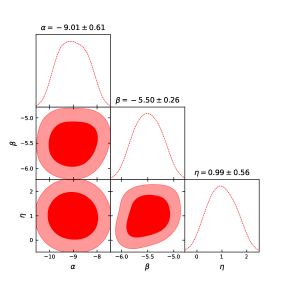
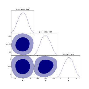
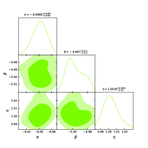
Figure 1: The $1\sigma$ and $2\sigma$ iso-likelihood contours for power-law $f(T,T_{G})$ cosmology, for the various two-dimensional subsets of the parameter space, for various datasets. The upper graph corresponds to the $Hubble$ dataset, the middle right corresponds to the $Pantheon$ dataset, and the lower graph corresponds to the joint analysis $Hubble+Pantheon$.

We perform the observational analysis described in the previous sections, and in Table 1 we provide the obtained results. Additionally, in Fig. 1 we depict the $1-\sigma$ and $2-\sigma$ confidence regions in various two-dimensional projections, obtained through contour analyses of $\chi^{2}$ in the parameter space [90].

Furthermore, in the upper graph of Fig. 2 we draw the Hubble parameter $H(z)$ in terms of the redshift $z$, using various datasets, while for completeness we add the corresponding curve for $\Lambda$CDM paradigm. The error bars depicted in the figure represent the uncertainties associated with the 55 data points utilized to construct the Hubble datasets. Similarly, the lower graph of Fig. 2 depicts the distance modulus $\mu(z)$ as a function of the redshift $z$, for the scenario at hand as well as $\Lambda$CDM cosmology, where the error bars represent the uncertainties associated with the Union 2.1 compilation.

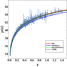
Figure 2: Upper graph: The Hubble parameter $H(z)$ in terms of the redshift $z$, using various datasets, where the error bars represent the uncertainties associated with the 55 data points utilized to construct the Hubble datasets. Lower graph: the distance modulus $\mu(z)$ as a function of the redshift $z$, where the error bars represent the uncertainties associated with the Union 2.1 compilation. For completeness, in both graphs we have added the corresponding curves for $\Lambda$CDM paradigm.

Finally, in Fig. 3 we present the reconstructed dark-energy equation of state given by (18). As we observe, $w_{DE}$ lies in the quintessence regime up to the present time, while in the future it experiences the phantom divide crossing. This capability was expected according to the form of (18), and it was discussed in [69].

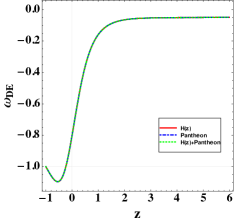
Figure 3: The evolution of the dark-energy equation-of-state parameter $w_{DE}$ given by (18), as a function of the redshift $z$, for the best-fit parameter obtained from various datasets.

IV Cosmographic analysis

In this section we perform a cosmographic analysis for $f({T},{T}_{{G}})$ cosmology. In particular, the dynamics of the late-time universe are examined through the utilization of the Hubble parameter, deceleration parameter, and jerk, snap, and lerk parameters [21]. Additionally, important information can be extracted by applying the $Om(z)$ Diagnostic [91]. In the following subsections, we investigate them in detail.

IV.1 Cosmographic parameters

The deceleration parameter is defined as

$$q=-1+(1+z)\frac{H^{\prime}}{H},$$ (29)

where primes denote derivatives with respect to redshift $z$, and it provides information about the acceleration rate of the universe, being positive during deceleration and negative during acceleration. Moreover, the jerk parameter is defined as [92, 93, 94],

$$j(z)=1-2(1+z)\frac{H^{\prime}}{H}+(1+z)^{2}\frac{H^{\prime 2}}{H^{2}}+(1+z)^{2}\frac{H^{\prime\prime}}{H}.$$ (30)

The sign of the jerk parameter $j$ determines how the dynamics of the universe change, with a positive value indicating the presence of a transition period during which the universe modifies its expansion. Additionally, the snap parameter is defined as [94]

$$\!\!\!\!\!\!\!\!\!\!\!\!\!\!\!\!\!\!s(z)=1-3(1\!+\!z)\frac{H^{\prime}}{H}+3(1\!+\!z)^{2}\frac{H^{\prime 2}}{H^{2}}+(1\!+\!z)^{3}\frac{H^{\prime 3}}{H^{3}}$$

$$\!-4(1\!+\!z)^{3}\frac{H^{\prime}H^{\prime\prime}}{H^{2}}+(1\!+\!z)^{2}\frac{H^{\prime\prime}}{H}-(1\!+\!z)^{3}\frac{H^{\prime\prime\prime}}{H},$$ (31)

while the lerk parameter as

$$\!\!\!\!\!\!\!\!\!\!\!\!l(z)=1-4(1\!+z\!)\frac{H^{\prime}}{H}+6(1\!+z\!)^{2}\frac{H^{\prime 2}}{H^{2}}-4(1\!+z\!)^{3}\frac{H^{\prime 3}}{H^{3}}$$

$$+(1\!+z\!)^{4}\frac{H^{\prime 4}}{H^{4}}-(1\!+z\!)^{3}\frac{H^{\prime}H^{\prime\prime}}{H^{2}}+7(1\!+z\!)^{4}\frac{H^{\prime}H^{\prime\prime\prime}}{H^{2}}$$

$$+11(1\!+z\!)^{4}\frac{H^{\prime 2}H^{\prime\prime}}{H^{3}}+2(1\!+z\!)^{2}\frac{H^{\prime\prime}}{H}+4(1\!+z\!)^{4}\frac{H^{\prime\prime 2}}{H^{2}}$$

$$+(1\!+z\!)^{3}\frac{H^{\prime\prime\prime}}{H}+(1\!+z\!)^{4}\frac{H^{\prime\prime\prime\prime}}{H},$$ (32)

both providing information on the higher-order derivatives of the Universe acceleration, offering insights into the transitions between different epochs. Notably, the snap parameter determines the extent to which the Universe evolution deviates from the one predicted by the $\Lambda$CDM model.

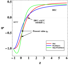
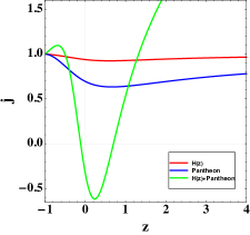
Figure 4: Upper graph: The evolution of the deceleration parameter as a function of the redshift. Lower graph: The evolution of the jerk parameter as a function of the redshift. In both graphs, we have used the best-fit parameter values obtained from various datasets.

In the upper panel of Fig. 4 we depict the evolution of the deceleration parameter $q$ as a function of the redshift $z$, for the model parameter values obtained from the observational analysis of the previous section. As we observe, we obtain a transition from deceleration to acceleration at late times, in the interval $0.52\leq z_{tr}\leq 0.89$, as expected. Concerning the present-time value $q_{0}$ it is found to be approximately $-0.60$ and $-0.68$ using the Hubble and Pantheon dataset, respectively, values that are consistent with the range of $q_{0}$ determined through recent observations [95, 96, 97, 98, 99].

The lower graph of Fig. 4 depicts the evolution of the jerk parameter. As we see, the current value of $j$ is approximated to be $j_{0}=0.93$ and $0.69$ using Hubble and Pantheon datasets respectively, aligning with recent analyses that establish constraints on the cosmographic coefficients [100, 101, 102], while in the far future $j$ approaches 1.

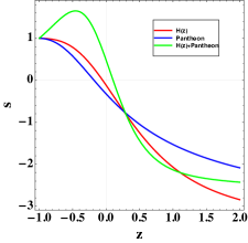
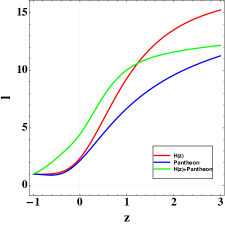
Figure 5: Upper graph: The evolution of the snap parameter as a function of the redshift. Lower graph: The evolution of the lerk parameter as a function of the redshift. In both graphs, we have used the best-fit parameter values obtained from various datasets.

Additionally, in the upper graph of Fig. 5 we present the evolution of the snap parameter $s(z)$, in which we observe a transition from a negative value to a positive value in the late stages. This behavior aligns with the preference of the scenario for quintessence-like behavior, indicated by $j\leq 1$ and $s>0$. Finally, in the lower graph of Fig. 5 we depict the lerk parameter as a function of the redshift. Notably, the lerk parameter rapidly decreases and stabilizes around $\simeq 1$. It is worth noting that, all the geometric parameters lie within the limits of cosmographic coefficients determined by late-time Universe analysis [21].

IV.2 $Om(z)$ Diagnostic

The $Om(z)$ geometrical diagnostic introduces an alternative way to differentiate the $\Lambda$CDM model from other dark energy models, bypassing the direct utilization of the equation of state [91]. In particular, it relies on the Hubble function and redshift, and it is written as

$$Om(z)=\frac{\left[\frac{H(z)}{H_{0}(z)}\right]^{2}-1}{z(z^{2}+3z+3)}.$$ (33)

When the slope of the $Om(z)$ trajectory is negative, it indicates that the dark energy behaves akin to quintessence. Conversely, a positive slope suggests that the dark energy exhibits phantom-like behavior. A zero slope, indicating a constant behavior of $Om(z)$, signifies that the dark energy corresponds to a cosmological constant ($\Lambda$CDM) [91]. In Fig. 6 we depict the evolution of $Om(z)$ as a function of the redshift. As we observe, the scenario of $f({T},{T}_{{G}})$ cosmology exhibits a quintessence-like behavior, in agreement with the previous results. Nevertheless, note that in the case of the Hubble function dataset, the behavior of the model is closer to that of the $\Lambda$CDM scenario.

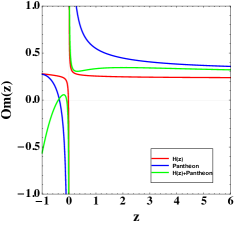
Figure 6: The evolution of the $Om(z)$ geometrical diagnostic as a function of the redshift, using the best-fit parameter values obtained from various datasets.

V Conclusions

We performed the observational confrontation and cosmographic analysis of $f({T},{T}_{{G}})$ gravity and cosmology. This higher-order torsional gravity is based on both the torsion scalar, as well as on the teleparallel equivalent of the Gauss-Bonnet combination, in its Lagrangian. Such a gravitational modification is different from both $f(R)$ and $F(G)$ curvature gravities, as well as from $f(T)$ torsional gravity, and it is known to have interesting cosmological applications. In particular, one obtains an effective dark-energy sector which depends on the extra torsion contributions.

Firstly, we employed the most recent observational data obtained from the Hubble function and SNeIa Pantheon datasets, in order to extract constraints on the free parameter space of power-law $f({T},{T}_{{G}})$ gravity. In particular, we applied a Markov Chain Monte Carlo sampling technique and we provided the $1\sigma$ and $2\sigma$ iso-likelihood contours, as well as the best-fit values for the parameters. As we saw, the scenario at hand is in agreement with observations. Additionally, we presented the variations of the Hubble parameter and the distance modulus the, acquired from the $H(z)$ dataset and the $1048$ data points of Pantheon respectively, where we showed that the variations of $H(z)$ and joint datasets are closer to $\Lambda$CDM cosmology, than the Pantheon one. Finally, drawing the effective dark-energy equation-of-state parameter we saw that we obtained a quintessence-like behavior, while in the future the Universe enters into the phantom regime, before it tends asymptotically to the cosmological constant value.

As a next step, we performed a detailed cosmographic analysis. From the behavior of the deceleration parameter, we showed that the transition from deceleration to acceleration occurs in the redshift range $0.52\leq z_{tr}\leq 0.89$. Additionally, the evolution of the jerk, snap, and lerk parameters showed the preference of the scenario at hand for a quintessence-like behavior. Finally, we applied the $Om(z)$ diagnostic analysis, and we observed that our model behaves like a quintessence model at late times, however in the case of the Hubble dataset the behavior of the model is closer to that of $\Lambda$CDM cosmology.

The above features reveal the capabilities of $f({T},{T}_{{G}})$ gravity and cosmology. Nevertheless, many tests need to be done before the scenario can be considered a good candidate for the description of nature. A necessary investigation is the detailed examination of the perturbations, and the study of the matter over density growth, since this will allow us to compare the scenario with data from Large-scale Structure, such as $f\sigma_{8}$ ones, and other perturbation-related probes. Furthermore, one should investigate the constraints on the theory from Solar-System experiments, since they are known to be very restrictive. These studies lie beyond the scope of the present work and are left for future projects.

- [1] E. J. Copeland, M. Sami and S. Tsujikawa, Int. J. Mod. Phys. D 15, 1753 (2006).
- [2] Y. F. Cai, E. N. Saridakis, M. R. Setare and J. Q. Xia, Phys. Rept. 493, 1 (2010).
- [3] B. A. Bassett, S. Tsujikawa and D. Wands, Rev. Mod. Phys. 78, 537-589 (2006)
- [4] E. N. Saridakis et al. [CANTATA], Springer, 2021, [arXiv:2105.12582 [gr-qc]].
- [5] S. Capozziello and M. De Laurentis, Phys. Rept. 509, 167 (2011).
- [6] E. Abdalla, G. Franco Abellán, A. Aboubrahim, A. Agnello, O. Akarsu, Y. Akrami, G. Alestas, D. Aloni, L. Amendola and L. A. Anchordoqui, et al. JHEAp 34, 49-211 (2022).
- [7] R. Alves Batista, G. Amelino-Camelia, D. Boncioli, J. M. Carmona, A. di Matteo, G. Gubitosi, I. Lobo, N. E. Mavromatos, C. Pfeifer and D. Rubiera-Garcia, et al. [arXiv:2312.00409 [gr-qc]].
- [8] A. A. Starobinsky, Phys. Lett. B 91, 99 (1980).
- [9] A. De Felice and S. Tsujikawa, Living Rev. Rel. 13, 3 (2010).
- [10] S. Nojiri and S. D. Odintsov, Phys. Lett. B 631, 1 (2005).
- [11] A. De Felice and S. Tsujikawa, Phys. Rev. D 80, 063516 (2009).
- [12] C. Erices, E. Papantonopoulos and E. N. Saridakis, Phys. Rev. D 99, no.12, 123527 (2019).
- [13] D. Lovelock, J. Math. Phys. 12, 498 (1971).
- [14] R. Aldrovandi and J. G. Pereira, Teleparallel Gravity, vol. 173. Springer Science+Business Media Dordrecht, 2013.
- [15] J. W. Maluf, Annalen Phys. 525, 339-357 (2013).
- [16] G. R. Bengochea and R. Ferraro, Phys. Rev. D 79, 124019 (2009).
- [17] Y. F. Cai, S. Capozziello, M. De Laurentis and E. N. Saridakis, Rept. Prog. Phys. 79, no.10, 106901 (2016).
- [18] J. M. Nester and H. J. Yo, Chin. J. Phys. 37, 113 (1999).
- [19] J. Beltrán Jiménez, L. Heisenberg and T. Koivisto, Phys. Rev. D 98, no.4, 044048 (2018).
- [20] L. Heisenberg,
- [21] K. Bamba, S. Capozziello, S. Nojiri and S. D. Odintsov, Astrophys. Space Sci. 342, 155-228 (2012).
- [22] S. Nojiri and S. D. Odintsov, Phys. Rept. 505, 59-144 (2011).
- [23] A. de la Cruz-Dombriz and D. Saez-Gomez, Class. Quant. Grav. 29, 245014 (2012).
- [24] T. Clifton, P. G. Ferreira, A. Padilla and C. Skordis, Phys. Rept. 513, 1-189 (2012).
- [25] S. Capozziello, F. S. N. Lobo and J. P. Mimoso, Phys. Lett. B 730, 280-283 (2014).
- [26] M. A. Skugoreva, E. N. Saridakis and A. V. Toporensky, Phys. Rev. D 91, 044023 (2015).
- [27] J. Gleyzes, D. Langlois, F. Piazza and F. Vernizzi, JCAP 02, 018 (2015).
- [28] S. Arai and A. Nishizawa, Phys. Rev. D 97, no.10, 104038 (2018).
- [29] T. Harko, F. S. N. Lobo, S. Nojiri and S. D. Odintsov, Phys. Rev. D 84, 024020 (2011).
- [30] J. K. Singh and R. Nagpal, Eur. Phys. J. C 80 (2020) no.4, 295.
- [31] J. K. Singh, Shaily and K. Bamba, Chin. J. Phys. 84 (2023), 371-380.
- [32] H. Shabani, A. De, T. H. Loo and E. N. Saridakis, [arXiv:2306.13324 [gr-qc]].
- [33] G. Cognola, E. Elizalde, S. Nojiri, S. D. Odintsov and S. Zerbini, Phys. Rev. D 73, 084007 (2006).
- [34] J. K. Singh, H. Balhara, K. Bamba and J. Jena, JHEP 03 (2023), 191 [erratum: JHEP 04 (2023), 049].
- [35] N. Chatzifotis, P. Dorlis, N. E. Mavromatos and E. Papantonopoulos, Phys. Rev. D 105, no.8, 084051 (2022).
- [36] J. K. Singh, Shaily, R. Myrzakulov and H. Balhara, New Astron. 104 (2023), 102070.
- [37] J. K. Singh, Shaily, A. Singh, A. Beesham and H. Shabani, Annals Phys. 455 (2023), 169382.
- [38] R. Lazkoz, F. S. N. Lobo, M. Ortiz-Baños and V. Salzano, Phys. Rev. D 100, no.10, 104027 (2019).
- [39] S. F. Yan, P. Zhang, J. W. Chen, X. Z. Zhang, Y. F. Cai and E. N. Saridakis, Phys. Rev. D 101, no.12, 121301 (2020)
- [40] S. Capozziello and R. D’Agostino, Phys. Lett. B 832, 137229 (2022).
- [41] N. Chatzifotis, P. Dorlis, N. E. Mavromatos and E. Papantonopoulos, Phys. Rev. D 107, no.8, 084053 (2023)
- [42] M. Koussour, S. Arora, D. J. Gogoi, M. Bennai and P. K. Sahoo, Nucl. Phys. B 990, 116158 (2023).
- [43] T. Karakasis, N. E. Mavromatos and E. Papantonopoulos, Phys. Rev. D 108, no.2, 024001 (2023).
- [44] S. Basilakos, D. V. Nanopoulos, T. Papanikolaou, E. N. Saridakis and C. Tzerefos, [arXiv:2307.08601 [hep-th]].
- [45] A. Bakopoulos, N. Chatzifotis, C. Erices and E. Papantonopoulos, JCAP 11, 055 (2023).
- [46] C. G. Boehmer, E. Jensko and R. Lazkoz, Universe 9, no.4, 166 (2023).
- [47] J. Beltrán Jiménez, L. Heisenberg, T. S. Koivisto and S. Pekar, Phys. Rev. D 101, no.10, 103507 (2020).
- [48] I. Ayuso, R. Lazkoz and V. Salzano, Phys. Rev. D 103, no.6, 063505 (2021).
- [49] F. Esposito, S. Carloni, R. Cianci and S. Vignolo, Phys. Rev. D 105, no.8, 084061 (2022).
- [50] M. Hohmann, C. Pfeifer, J. Levi Said and U. Ualikhanova, Phys. Rev. D 99, no.2, 024009 (2019).
- [51] M. Hohmann, Phys. Rev. D 104, no.12, 124077 (2021).
- [52] J. Beltrán Jiménez, L. Heisenberg and T. S. Koivisto, JCAP 08, 039 (2018).
- [53] J. Lu, X. Zhao and G. Chee, Eur. Phys. J. C 79, no.6, 530 (2019).
- [54] F. D’Ambrosio, L. Heisenberg and S. Kuhn, Class. Quant. Grav. 39 (2022) no.2, 025013.
- [55] A. R. P. Moreira, J. E. G. Silva, F. C. E. Lima and C. A. S. Almeida, Phys. Rev. D 103, no.6, 064046 (2021).
- [56] F. K. Anagnostopoulos, S. Basilakos and E. N. Saridakis, Phys. Lett. B 822, 136634 (2021).
- [57] L. Atayde and N. Frusciante, Phys. Rev. D 104, no.6, 6 (2021).
- [58] F. D’Ambrosio, S. D. B. Fell, L. Heisenberg and S. Kuhn, Phys. Rev. D 105, no.2, 024042 (2022).
- [59] D. Zhao, Eur. Phys. J. C 82, no.4, 303 (2022).
- [60] A. De and L. T. How, Phys. Rev. D 106, no.4, 048501 (2022).
- [61] R. H. Lin and X. H. Zhai, Phys. Rev. D 103, no.12, 124001 (2021) [erratum: Phys. Rev. D 106, no.6, 069902 (2022)].
- [62] B. J. Barros, T. Barreiro, T. Koivisto and N. J. Nunes, Phys. Dark Univ. 30, 100616 (2020).
- [63] Á. D. Kovács and H. S. Reall, Phys. Rev. D 101, no.12, 124003 (2020).
- [64] M. Caruana, G. Farrugia and J. Levi Said, Eur. Phys. J. C 80, no.7, 640 (2020).
- [65] W. Khyllep, A. Paliathanasis and J. Dutta, Phys. Rev. D 103, no.10, 103521 (2021).
- [66] S. Bahamonde, C. G. Böhmer and M. Wright, Phys. Rev. D 92, no.10, 104042 (2015).
- [67] A. De, T. H. Loo and E. N. Saridakis, [arXiv:2308.00652 [gr-qc]].
- [68] G. Kofinas and E. N. Saridakis, Phys. Rev. D 90, 084044 (2014).
- [69] G. Kofinas and E. N. Saridakis, Phys. Rev. D 90, 084045 (2014).
- [70] S. Capozziello, M. De Laurentis and K. F. Dialektopoulos, Eur. Phys. J. C 76, no.11, 629 (2016).
- [71] Á. de la Cruz-Dombriz, G. Farrugia, J. L. Said and D. Sáez-Chillón Gómez, Phys. Rev. D 97, no.10, 104040 (2018).
- [72] S. Chattopadhyay, A. Jawad, D. Momeni and R. Myrzakulov, Astrophys. Space Sci. 353, no.1, 279-292 (2014).
- [73] M. Zubair and A. Jawad, Astrophys. Space Sci. 360, 11 (2015).
- [74] M. Sharif and K. Nazir, Mod. Phys. Lett. A 32, no.13, 1750083 (2017).
- [75] G. Mustafa, G. Abbas and T. Xia, Chin. J. Phys. 60, 362-378 (2019).
- [76] P. Asimakis, S. Basilakos, N. E. Mavromatos and E. N. Saridakis, Phys. Rev. D 105, no.8, 084010 (2022).
- [77] Á. de la Cruz-Dombriz, G. Farrugia, J. L. Said and D. Saez-Gomez, Class. Quant. Grav. 34, no.23, 235011 (2017).
- [78] S. V. Lohakare, B. Mishra, S. K. Maurya and K. N. Singh, Phys. Dark Univ. 39, 101164 (2023).
- [79] S. Bahamonde and C. G. Böhmer, Eur. Phys. J. C 76, no.10, 578 (2016).
- [80] S. Bahamonde, K. F. Dialektopoulos, C. Escamilla-Rivera, G. Farrugia, V. Gakis, M. Hendry, M. Hohmann, J. Levi Said, J. Mifsud and E. Di Valentino, Rept. Prog. Phys. 86 (2023) no.2, 026901.
- [81] S. A. Kadam, B. Mishra and J. Levi Said, Phys. Scripta 98, no.4, 045017 (2023).
- [82] S. Capozziello, A. Stabile and A. Troisi, Class. Quant. Grav. 24, 2153-2166 (2007).
- [83] A. Paliathanasis, S. Basilakos, E. N. Saridakis, S. Capozziello, K. Atazadeh, F. Darabi and M. Tsamparlis, Phys. Rev. D 89, 104042 (2014).
- [84] A. De Felice and S. Tsujikawa, Phys. Lett. B 675, 1-8 (2009).
- [85] A. Jawad, S. Chattopadhyay and A. Pasqua, Eur. Phys. J. Plus 128, 88 (2013).
- [86] D. Foreman-Mackey, D. W. Hogg, D. Lang and J. Goodman, Publ. Astron. Soc. Pac. 125, 306-312 (2013).
- [87] D. M. Scolnic et al. [Pan-STARRS1], Astrophys. J. 859, no.2, 101 (2018).
- [88] G. S. Sharov and V. O. Vasiliev, Math. Model. Geom. 6 (2018), 1-20.
- [89] L. Chimento and M. I. Forte, Phys. Lett. B 666 (2008), 205-211.
- [90] J. K. Singh, Shaily, S. Ram, J. R. L. Santos and J. A. S. Fortunato, Int. J. Mod. Phys. D 32 (2023) no.07, 2350040.
- [91] V. Sahni, A. Shafieloo and A. A. Starobinsky, Phys. Rev. D 78, 103502 (2008).
- [92] M. Visser, Gen. Rel. Grav. 37, 1541-1548 (2005).
- [93] D. Rapetti, S. W. Allen, M. A. Amin and R. D. Blandford, Mon. Not. Roy. Astron. Soc. 375, 1510-1520 (2007).
- [94] J. Liu, L. Qiao, B. Chang and L. Xu, Eur. Phys. J. C 83, no.5, 374 (2023).
- [95] N. G. Busca, T. Delubac, J. Rich, S. Bailey, A. Font-Ribera, D. Kirkby, J. M. Le Goff, M. M. Pieri, A. Slosar and E. Aubourg, et al. Astron. Astrophys. 552 (2013), A96.
- [96] O. Farooq and B. Ratra, Astrophys. J. Lett. 766, L7 (2013).
- [97] S. Capozziello, O. Farooq, O. Luongo and B. Ratra, Phys. Rev. D 90, no.4, 044016 (2014).
- [98] C. Gruber and O. Luongo, Phys. Rev. D 89, no.10, 103506 (2014).
- [99] Y. Yang and Y. Gong, JCAP 06, 059 (2020).
- [100] A. Aviles, C. Gruber, O. Luongo and H. Quevedo, Phys. Rev. D 86 (2012), 123516.
- [101] A. Aviles, A. Bravetti, S. Capozziello and O. Luongo, Phys. Rev. D 90 (2014) no.4, 043531.
- [102] S. Capozziello, O. Luongo and E. N. Saridakis, Phys. Rev. D, 91 (2015) no.12, 124037.