Transformer-Based Multi-Object Smoothing with Decoupled Data Association and Smoothing

Abstract

Multi-object tracking (MOT) is the task of estimating the state trajectories of an unknown and time-varying number of objects over a certain time window. Several algorithms have been proposed to tackle the multi-object smoothing task, where object detections can be conditioned on all the measurements in the time window. However, the best-performing methods suffer from intractable computational complexity and require approximations, performing suboptimally in complex settings. Deep learning based algorithms are a possible venue for tackling this issue but have not been applied extensively in settings where accurate multi-object models are available and measurements are low-dimensional. We propose a novel DL architecture specifically tailored for this setting that decouples the data association task from the smoothing task. We compare the performance of the proposed smoother to the state-of-the-art in different tasks of varying difficulty and provide, to the best of our knowledge, the first comparison between traditional Bayesian trackers and DL trackers in the smoothing problem setting.

Multi-object smoothing, Deep Learning, Transformers, Random Finite Sets.

1 INTRODUCTION

The objective of multi-object tracking (MOT) is to estimate the state trajectories of an unknown and time-varying number of objects based on a sequence of noisy sensor measurements. The objects can enter and leave the field-of-view (FOV) at any time, there might be missed detections, and there might be false measurements originating from sensor noise and/or clutter. Being able to achieve high performance in this task is of high importance and has applications in many different contexts, such as pedestrian tracking [1], autonomous driving [2], sports players tracking [3], defense systems [4], animal tracking [5, 6], and more.

For some applications, the set of trajectories is to be estimated using only measurements available until the most recent time, which can then be used by real-time decision systems downstream (e.g., autonomous driving, defense systems) [7]. In other applications, all of the measurements in a time window are available when estimating the trajectories (e.g., examining animal behavior recorded in the past, analysis of autonomous driving accidents), and algorithms can condition the estimated trajectories to all of the measurements available, yielding (smoothed) estimates of superior quality [8]. This latter formulation will henceforth be referred to as multi-object smoothing.

Several algorithms have been proposed to tackle the multi-object smoothing task. Two important classes are trackers based on approximations of the multi-object density, such as the trajectory Probability Hypothesis Density (PHD) smoothing and trajectory cardinalized PHD smoothing [9], and trackers based on multi-object conjugate priors, such as the generalized labeled multi-Bernoulli [10], and the multi-scan trajectory Poisson multi-Bernoulli mixture (TPMBM) [11, 12, 13]. Trackers based on multi-object conjugate priors provide closed-form solutions to the task for certain classes of multi-object models. However, due to the unknown measurement-object associations, these approaches suffer from a computational complexity that is super-exponential in the number of time-steps being processed [7]. This drawback requires them to resort to heuristics such as pruning or merging to maintain computational tractability, which negatively impact performance in challenging scenarios. In addition, if the multi-object models contain nonlinearities, such methods must employ sequential Monte Carlo methods or Gaussian approximations to be able to function, which may further impair tracking quality [14].

One appealing direction to improve these methods’ shortcomings is using deep learning (DL). DL-based algorithms are able to leverage vast amounts of data to learn a variety of complex input-output mappings, such as classifying images [15], translating text [16], super-human level of play in classic games [17], and even generating realistic images from text prompts [18], so it is plausible that such approaches would be helpful in the MOT context too. Indeed, deep learning has been increasingly applied to the field of MOT, resulting in breakthroughs in state-of-the-art performance [19, 20, 21, 22]. Initially, DL was used mostly as an aid to solving certain subtasks, such as associating new measurements to existing tracks [23], managing track initialization/termination [24], and predicting motion models [25], to name a few. More recent approaches use DL to solve the entire (or almost the entire) MOT task, with architectures based on object detector extensions [26], convolutional neural networks [27, 28, 29, 30, 31], graph neural networks [32, 33, 34] or, more recently, the transformer network [35, 36, 37, 38, 39, 40].

Although such approaches have seen success and widespread adoption in contexts where the measurements are high-dimensional and the multi-object models are too complicated to be modeled accurately (e.g., tracking with video sequences), a setting henceforth referred to as model-free, the same cannot be said about the counterpart situation when there are accurate multi-object models available, and the measurements are low-dimensional (e.g., radar tracking of aircraft). In this setting, which we will refer to as the model-based setting, random finite sets (RFS) methods based on conjugate priors have been shown to present excellent tracking performance [11], but with few exceptions [41], there have been no comparisons between the performance of such methods and DL methods based on recent advancements such as the transformer [42] architecture, especially for the smoothing task.

This paper proposes a novel DL multi-object tracker specifically tailored for the model-based setting, named Deep Decoupled Data Association and Smoothing (D3AS). Its architecture tackles the smoothing problem formulation by leveraging the recent transformer neural network structure [42] for efficient use of the entire measurement sequence when performing predictions. Importantly, it decouples the data association task (reasoning about the unknown association between measurements and objects) from the filtering/smoothing task (predicting trajectories given associations), which reduces training time and model size, and results in more interpretable predictions. We compare the performance of the proposed tracker to TPMBM [12, 11], which presents state-of-the-art smoothing performance [13, Section VIII], in tasks of varying difficulty. To the best of our knowledge, we provide the first results indicating that a deep-learning smoother can outperform model-based Bayesian trackers such as TPMBM in complex tasks. Our specific contributions are:

• Propose a novel transformer-based module for the data association task, and the loss formulation for training it independently from the smoothing task.

• Propose a novel transformer-based module for the smoothing task, based on recent advancements of large language models [43]. In specific, this model takes as input a sequence of measurements and corresponding confidences and predicts a smoothed trajectory.

• Perform a thorough comparison between the proposed deep learning smoother and the state-of-the-art smoother TPMBM in various settings of different complexity, reporting that DL methods can outperform traditional model-based models in challenging scenarios.

Notations

In this paper we use the following notations: Scalars are denoted by lowercase or uppercase letters with no special typesetting ($x$), vectors by boldface lowercase letters ($\mathbf{x}$), sets by blackboard-bold uppercase letter ($\mathbb{X}$), and matrices by boldface uppercase letters ($\mathbf{X}$). The element in the $i$-th row and $j$-th column of a matrix $\mathbf{A}$ is denoted $\mathbf{A}_{i,j}$. Sequences are indicated by adding subscripts denoting their ranges to the typesetting that matches their elements (e.g., $\mathbf{x}_{1:k}$ is a sequence of vectors, $\mathbb{X}_{1:j}$ of sets). The number of elements in a set $\mathbb{X}$ is denoted $|\mathbb{X}|$, and we further define $\mathbb{N}_{a}\triangleq\{i~{}:~{}i\leq a~{},~{}i\in\mathbb{N}\}$.

2 MULTI-OBJECT MODELS AND PROBLEM FORMULATION

2.1 Multi-Object Models

The state vector for an object at time-step $t$ is denoted $\mathbf{x}_{t}\in\mathbb{R}^{d_{x}}$, and its trajectory is represented by a tuple $\bm{\tau}=(t_{s},\mathbf{x}_{t_{s}:t_{s}+l})$, where $t_{s}$ is the initial time in which the object entered the FOV, and $l$ is the number of time-steps it was present for. We use superscripts to specify a certain object $i$, such as $\mathbf{x}_{t}^{i}$ for its state at time $t$. The set of trajectories of all objects inside the FOV at any time-step between $0$ and $T$ is denoted $\mathbb{T}_{T}$. We use the standard multi-object dynamic models [44, Chap.5]. The birth model is a Poisson point process (PPP) with state-dependent intensity function $\lambda_{b}(\mathbf{x})$, and object death is modeled as independent and identically distributed (i.i.d.) Markovian processes with survival probability $p_{s}(\mathbf{x})$. Object motion is also modeled as i.i.d. Markovian, where the single-object transition model is denoted $f(\mathbf{x}_{t+1}|\mathbf{x}_{t})$.

We also use the standard measurement models, with the point-object assumption [44, Chap.5]. Measurements originating from objects are generated independently for each object, where each object can generate at most one measurement per time-step with probability of detection $p_{d}(\mathbf{x})$, and each measurement $\mathbf{z}_{t}\in\mathbb{R}^{d_{z}}$ originates from at most one object. We denote the single-object measurement likelihood as $g(\mathbf{z}_{t}|\mathbf{x}_{t})$, and model clutter as a PPP with constant intensity function $\lambda_{c}(\cdot)$ over the field of view (FOV). The set of all measurements generated at time-step $t$ is denoted $\mathbb{Z}_{t}$.

2.2 Problem Formulation

We focus on the problem of multi-object smoothing for a window of $T$ time-steps. We are given a tuple of measurement sets $(\mathbb{Z}_{1},\cdots,\mathbb{Z}_{T})$ with arbitrary length $T$, and are tasked with estimating the set of object trajectories $\mathbb{T}_{T}$. As an example, the tuple of measurement sets could be generated from a radar or LIDAR sensor mounted on top of a vehicle, and $\mathbb{T}_{T}$ represents the trajectories of, e.g., pedestrians, cars, and cyclists.

To train a DL solution, we first approximate the multi-object posterior density of $\mathbb{T}_{T}$ given $(\mathbb{Z}_{1},\cdots,\mathbb{Z}_{T})$ as a $B$-component multi-Bernoulli RFS density, where each Bernoulli component $i$ has an existence probability $\bar{p}^{i}$ and corresponds to one (potential) trajectory. The trajectory for Bernoulli component $i$ is parameterized as a tuple of the form $(\hat{\mathbf{x}}_{1:T}^{i},p_{1:T}^{i})$, where $\hat{\mathbf{x}}_{1:T}^{i}\in\mathbb{R}^{d_{x}\times T}$ is a state sequence of length $T$, and $p_{1:T}^{i}\in[0,1]^{T}$ are per-time-step existence probabilities.

Then, we create the set $\mathbb{Z}_{\Omega}$, containing the measurements from all time-steps, together with their times-of-arrival

$$\mathbb{Z}_{\Omega}=\bigcup_{t=1}^{T}\big{\{}(\mathbf{z},t):\mathbf{z}\in\mathbb{Z}_{t}\big{\}}~{},$$ (1)

and learn models that take as input $\mathbb{Z}_{\Omega}$ and output the parameters $\{\hat{\mathbf{x}}_{1:T}^{i},p_{1:T}^{i},\bar{p}^{i}\}_{i=1}^{B}$ describing the multi-Bernoulli density. In effect, this casts the multi-object smoothing task as a set-to-set prediction task. We also note that the use of existence probabilities $\bar{p}$ allows the models to predict a variable number of trajectories (no larger than $B$), since excess trajectories can have their corresponding $\bar{p}$ set to zero. At the same time, the per-time-step existence probabilities $p_{1:T}$ allow for variable-length trajectories since excess time-steps can have their corresponding $p_{t}$ set to zero. For example, if $p_{t}^{i}=0$ only for $t>t_{\text{end}}$, then trajectory $i$ is considered to end at time-step $t_{\text{end}}$, and is only $t_{\text{end}}$ time-steps long (instead of $T$). In this case, $\hat{\mathbf{x}}_{t_{\text{end}}+1:T}$ can be arbitrary vectors not considered part of the trajectory.

3 BACKGROUND ON TRANSFORMERS

This section reviews the transformer encoder architecture used in both the data association and the smoothing modules of D3AS to process sequences of measurements. The transformer model is a popular and successful neural network architecture specifically tailored for sequence-to-sequence learning tasks. Originally proposed in [42], its structure is comprised of an encoder and a decoder, but in this paper only the encoder will be reviewed, as this is the only part used in D3AS. The transformer encoder is in charge of processing an input sequence $\mathbf{a}_{1:n}$, into a new representation $\mathbf{e}_{1:n}$, referred to as the embeddings of the input sequence, where both $\mathbf{a}_{i},\mathbf{e}_{i}\in\mathbb{R}^{d}$ for $i\in\mathbb{N}_{n}$. After training, the encoder generates embeddings such that each $\mathbf{e}_{i}$ encodes the value of the corresponding $\mathbf{a}_{i}$ and its relationship to all other elements of the input sequence. Once the embeddings have been computed by the encoder, they can be used by downstream modules that require a global understanding of all elements $\mathbf{a}_{1:n}$ and their relationships.

3.1 Multihead Self-attention

The main building block behind the power of transformer architectures is the self-attention layer. This layer processes a sequence $\mathbf{a}_{1:n}$ into a sequence $\mathbf{b}_{1:n}$ ($\mathbf{a}_{i},\mathbf{b}_{i}\in\mathbb{R}^{d}$ for $i\in\mathbb{N}_{n}$), and is stacked multiple times inside a transformer encoder. The processing of a self-attention layer starts with the computation of three different linear combinations of the input, namely

$$\mathbf{Q}=\mathbf{W}_{Q}\mathbf{A},~{}\mathbf{K}=\mathbf{W}_{K}\mathbf{A},~{}\mathbf{V}=\mathbf{W}_{V}\mathbf{A},$$ (2)

where $\mathbf{A}=\begin{bmatrix}\mathbf{a}_{1},\cdots,\mathbf{a}_{n}\end{bmatrix}\in\mathbb{R}^{d\times n}$, and the matrices $\mathbf{Q},\mathbf{K},\mathbf{V}$ are referred to as queries, keys, and values, respectively. The matrices $\mathbf{W}_{Q},\mathbf{W}_{K},\mathbf{W}_{V}\in\mathbb{R}^{d\times d}$ are the learnable parameters of the self-attention layer. Then, the output is computed as

$$\mathbf{B}=\mathbf{V}~{}\text{Softmax-c}\left(\frac{\mathbf{K}^{\top}\mathbf{Q}}{\sqrt{d}}\right)~{},$$ (3)

where $\mathbf{B}=\begin{bmatrix}\mathbf{b}_{1},\cdots,\mathbf{b}_{n}\end{bmatrix}\in\mathbb{R}^{d\times n}$ and Softmax-c is the column-wise application of the Softmax function to a matrix, defined as

$$[\text{Softmax-c}(\mathbf{M})]_{i,j}=\frac{e^{m_{i,j}}}{\sum_{k=1}^{d}e^{m_{k,j}}};\quad i,j\in\mathbb{N}_{n}$$

for a matrix $\mathbf{M}\in\mathbb{R}^{n\times n}$, where $c_{i,j}$ is the element of $\mathbf{M}$ on row $i$, column $j$.

Additionally, most transformer-based models (including D3AS) use several self-attention layers in parallel and combine the results, referring to the combined computation as a multihead self-attention layer. Concretely, $\mathbf{A}$ is fed to $n_{h}$ different self-attention layers with separate learnable parameters, generating $n_{h}$ different outputs $\mathbf{B}_{1},\cdots,\mathbf{B}_{n_{h}}$.The final output $\mathbf{B}$ is then computed by vertically stacking the results and applying a linear transformation to reduce the dimensionality back to $\mathbb{R}^{d\times n}$:

$$\mathbf{B} =\mathbf{W}^{0}\begin{bmatrix}\mathbf{B}_{1}\\ \vdots\\ \mathbf{B}_{n_{h}}\end{bmatrix}~{},$$ (4)

where $\mathbf{W}^{0}\in\mathbb{R}^{d\times dn_{n}}$ is a learnable parameter of the multi-head self-attention layer.

3.2 Transformer Encoder

Figure 1: The structure of the transformer encoder proposed in [45], where $N$ encoder blocks are connected in series. The components of each encoder block are shown on the right.

Stacking several layers of multiheaded self-attention allows models to learn complicated long-term dependencies in input sequence. The transformer encoder does exactly this, interleaving multiheaded self-attention layers with other types of nonlinearities. In this paper, we use a slightly modified version of the encoder, proposed in [45], as shown in Fig. 1. The overall encoder is built by stacking $N$ “encoder blocks”, where the output from one block is fed to the next. The computation for encoder block $l\in\mathbb{N}_{N}$ can be described as

$$\tilde{\mathbf{a}}_{1:n}^{(l-1)}=\mathbf{a}_{1:n}^{(l-1)}+\mathbf{q}_{1:n}$$ (5)

$$\mathbf{b}^{(l)}_{1:n}=\mathrm{MultiHeadAttention}(\tilde{\mathbf{a}}_{1:n}^{(l-1)})$$ (6)

$$\tilde{\mathbf{b}}^{(l)}_{1:n}=\mathrm{LayerNorm}(\tilde{\mathbf{a}}_{1:n}^{(l-1)}+\mathbf{b}^{(l)}_{1:n})$$ (7)

$$\mathbf{a}_{1:n}^{(l)}=\mathrm{LayerNorm}(\tilde{\mathbf{b}}^{(l)}_{1:n}+\text{FFN}(\tilde{\mathbf{b}}^{(l)}_{1:n}))~{},$$ (8)

where MultiHeadAttention is a multi-head self-attention layer, FFN is a fully-connected feedforward neural network applied to each element of the input sequence separately, and LayerNorm is a Layer Normalization layer [46]. We use the notation $\mathbf{a}_{1:n}^{(l)}$ to denote the input sequence after being processed by $l$ encoder blocks. For instance, $\mathbf{a}_{1:n}^{(0)}$ is the original input sequence $\mathbf{a}_{1:n}$, and $\mathbf{a}_{1:n}^{(N)}$ is the output of the encoder module, also denoted $\mathbf{e}_{1:n}$. Additionally, at the start of every encoder block, the sequence $\mathbf{z}_{1:n}^{(l)}$ is added with a vector $\mathbf{q}_{1:n}$, referred to as the positional encoding, which can be either fixed (usually with sinusoidal components) [42] or learnable [45]. Without this addition, the encoder would become permutation-equivariant, which is undesirable in many contexts that rely on the relative position of the elements $\mathbf{a}_{i}$ in $\mathbf{a}_{1:n}$ to convey important information.

4 METHOD

This section describes D3AS, the proposed method for performing multi-object smoothing in the model-based context. It is divided into two modules: the Deep Data Associator (DDA) and the Deep Smoother (DS).

4.1 Overview of DDA and DS modules

Figure 2 shows an example of the method processing a measurement sequence into trajectories. On the left of the image, a measurement sequence $\mathbf{z}_{1:n}$ with eight measurements is shown, which is fed to the DDA module. This module attends to all measurements simultaneously and predicts the data association matrix $\mathbf{A}\in\mathbb{R}^{n\times B}$, where each row corresponds to one probability mass function (pmf) over $B$ possible tracks. Each column of the matrix corresponds to one track, where $B=4$ in this example. This matrix can be interpreted as a soft, trainable association between measurements and tracks. Connecting the DDA’s module output to the next module’s input is a partitioning step, which uses the predicted data association matrix to partition the measurements into $B$ different tracks. This step also discards tracks that do not have any associated measurements (e.g., track 4 in Fig. 2).Each remaining track is then individually fed to the DS module, shown in green on the right, which processes the measurements in each track into the corresponding parameters $(\hat{\mathbf{x}}_{1:T},p_{1:T},\bar{p})$ of its predicted trajectory.

Decoupling the data association from the smoothing task brings many benefits. Evidently, it increases the interpretability of the model by providing access to the data associations used, allowing users to better understand the predictions and diagnose, e.g., if a bad prediction was due to incorrect data associations or because the smoothing process was not able to provide reasonable estimates. However, added interpretability is not the only advantage. Many transformer-based multi-object trackers rely on the transformer decoder to produce estimates, but the involved cross-attention and object query training have been associated with slow convergence [47, 48, 49, 50, 51]. By decoupling the data association from smoothing, D3AS sidesteps the need for a decoder, which reduces training time, inference time, and model size.

Figure 2: Overview of the DDA+DS method. A scene containing a sequence of measurements is processed by the DDA, which produces a data association matrix. This is then used for partitioning (represented by the box P) the measurement sequence, and each partition is individually fed to the deep smoother module for predicting a track.

4.2 Deep Data Association Module

The high-level functioning of the DDA module is shown in Fig. 3. First, the measurements in the set $\mathbb{Z}_{\Omega}$ are put in arbitrary order in a sequence $\mathbf{z}_{1:n}$, and the corresponding times-of-arrival in the same order are put into another sequence $t_{1:n}$. Then, we project each element of the sequence $\mathbf{z}_{i}$ into a higher-dimensional representation $\mathbf{z}^{\prime}_{i}\in\mathbb{R}^{d^{\prime}}$ with the help of an FFN layer, and use a transformer encoder to process this new measurement sequence into embeddings $\mathbf{e}_{1:n}$.

For the encoder to know when each measurement was obtained, we use positional encodings based on the time-of-arrival of the measurements, as introduced in (1). In specific, the positional encoding $\mathbf{q}_{i}$ used by the DDA’s encoder for element $i$ of the input sequence is based on the time-of-arrival for that measurement: $\mathbf{q}_{i}=f(t_{i})$, where $f$ is a learnable lookup table trained jointly with the other DDA’s learnable parameters.

Using a transformer encoder allows the DDA to efficiently learn complex temporal dependencies between all the measurements, enabling powerful data association predictions conditioned on the entire set $\mathbb{Z}_{\Omega}$. After the encoder, each embedding is individually fed to a feedforward neural network (FFN) and a Softmax (SM) layer, resulting in a pmf $\mathbf{y}_{i}$ for each measurement $\mathbf{z}_{i}$, which are used to form the rows of $\mathbf{A}$, i.e., $\mathbf{A}=\begin{bmatrix}\mathbf{y}_{1}^{\top}&\cdots&\mathbf{y}_{n}^{\top}\end{bmatrix}^{\top}$. The DDA module is fully trainable, and we propose a novel loss to allow supervised training of the prediction $\mathbf{A}$, described in subsection 4.5.

Figure 3: Structure of the Deep Data Associator module. A sequence of measurements $\mathbf{z}_{1:n}$ is processed by a transformer encoder that uses temporal encodings, followed by an individual application of FFN and Softmax layers to the computed embedding for each measurement.

4.3 Partitioning

The partitioning step in D3AS uses the predicted data association matrix to decide how to partition the measurement sequence $\mathbf{z}_{1:n}$ before feeding it to the DS module. We find that a simple greedy assignment performs reasonably well in the cases studied, compared to the model-based benchmark: each measurement is associated to the track corresponding to the mode of its predicted pmf, and tracks that end up without any measurements are discarded. To provide a proxy for how much the smoother should trust each measurement, we concatenate the maximum value of each measurement’s association pmf to the measurement vector. Further, by using the time-of-arrival information of each measurement, we sort them in arrival order into a sequence and add a dummy vector $\tilde{\mathbf{z}}$ to all the time-steps where a track does not have measurements. If multiple measurements with the same time-of-arrival end up in the same track, we remove all but one of them. These two steps enforce all tracks to have exactly $T$ elements, regardless of how many measurements that track contains.

A sample output of this process is illustrated in Fig. 2, showing the partitioning of the measurements into four different tracks. Time-steps with missing measurements (e.g., the first four time-steps for track 1) use a dummy $\tilde{\mathbf{z}}$ vector, and the DS module will be given the information that measurement $\mathbf{z}_{1}$ is less certain than the others (illustrated by making the box underneath it less opaque).

4.4 Deep Smoother Module

Figure 4: Structure of the Deep Smoother module. A sequence of measurements from a track is processed into a state trajectory $\hat{\mathbf{x}}_{1:T}$, existence probabilities $p_{1:T}$, and a global trajectory existence probability $\bar{p}$.

The DS module is in charge of processing each track of measurements into the parameters of the output multi-Bernoulli density of trajectories, i.e., $\{\hat{\mathbf{x}}_{1:T}^{i},p_{1:T}^{i},\bar{p}^{i}\}_{i=1}^{B}$. To achieve this, we use a transformer encoder for processing a track’s measurements, followed by nonlinearities applied to each time-step. Fig. 4 illustrates the application of the DS module to the track shown in the top-right of Fig. 2. The encoder generates an embedding sequence $\mathbf{e}_{1:T}$ ($T=5$ in the example), and each embedding is fed to a separate head for predicting the state $\hat{\mathbf{x}}_{t}$ and the auxiliary existence variable $p_{t}$ at each time-step $t$. The encoder uses its self-attention to efficiently attend to all measurements in a track when predicting $(\hat{\mathbf{x}}_{t},p_{t})$, $t\in\mathbb{N}_{T}$. To deal with time-steps with missing measurements, we draw inspiration from Masked Language Modeling [43] and feed a dummy vector $\tilde{\mathbf{z}}_{\text{DS}}$ to all such time-steps. Similar to the DDA module, the measurements (with confidences) are projected into a higher-dimensional representation with the help of an FFN before feeding them to the encoder (not shown in the figure to avoid clutter).

Besides predicting $\hat{\mathbf{x}}_{1:T}$ and $p_{1:T}$, the DS module also outputs the existence probability $\bar{p}$ for the track’s estimated trajectory. This is accomplished by concatenating all the track’s measurements (along with confidences) into a high-dimensional vector and feeding it to an FFN, as shown in Fig. 4. This allows the smoother to, for instance, decide if a track contains only false measurements and should be discarded.

4.5 Losses

This section describes the two losses used to train D3AS, one for specifically supervising the data association output and one for the parameters of the multi-Bernoulli density of trajectories.

4.5.1 Deep Data Associator Loss

In order to train the DDA module, we need a loss $\mathcal{L}_{\text{DDA}}$ that supervises the predicted association matrix $\mathbf{A}$ using the measurements $\mathbf{z}_{1:n}$ and the ground-truth information of which object each measurement came from. This loss should penalize associations where measurements from the same object are put into different tracks, as well as associations where measurements from different objects are put into the same track. At the same time, it should be invariant to the order of the columns in the association matrix $\mathbf{A}$, since such order is arbitrary from the point of view of the final predicted data associations. Lastly, it is also necessary that the loss is differentiable with respect to the model’s parameters, and desirable that it is easy and stable to optimize with algorithms like stochastic gradient descent.

During training, we assume we know which measurements originate from the same object. Based on this knowledge, we can formulate a ground-truth association matrix $\mathbf{A}^{*}$ where each column corresponds to a unique object and each row is a one-hot vector. Measurements from the same object have 1’s in the same column, and false measurements are treated as all coming from the same object (different from all the other objects). We can then use cross-entropy as a loss function for training $\mathbf{A}$:

$$\mathcal{L}_{\text{DDA}}(\mathbf{A},\mathbf{A}^{*})=-\frac{1}{N}\sum_{i=1}^{N}\sum_{j=1}^{B}\log(\mathbf{A}_{i,j})\cdot\mathbf{A}^{*}_{i,j}~{}.$$ (9)

To obtain a loss function that is invariant to how we order the columns in $\mathbf{A}$, we can select $\mathbf{A}^{*}$ by ordering its columns to match the tracks predicted by $\mathbf{A}$. This can be done by solving a minimum cost assignment between tracks and objects, where the cost of matching a track to an object is related to how much mass of measurements from that object the matrix $\mathbf{A}$ has put on that track.

Concretely, we first solve the following assignment between $B$ tracks and $|\mathbb{T}_{T}|$ objects:

$$\mathbf{S}^{*}=\arg\min_{\mathbf{S}} \sum_{j=1}^{B}\sum_{k=1}^{|\mathbb{T}_{T}|}\mathbf{S}_{j,k}\cdot\mathbf{C}_{j,k}~{},$$ (10)

where $\mathbf{S}$ is an assignment matrix subject to the constraints

$$\sum_{j=1}^{B}\mathbf{S}_{j,k}=1,\quad\mathbf{S}_{j,k}\in\{0,1\}~{},$$ (11)

for all $j\in\mathbb{N}_{B}$, and all $k\in\mathbb{N}_{|\mathbb{T}_{T}|}$. The cost matrix $\mathbf{C}$ is defined as

$$\mathbf{C}_{j,k}=-\sum_{i=1}^{n}\mathbf{A}_{i,j}\cdot\mathbb{I}(b_{i}=k)~{},$$ (12)

where $\mathbb{I}(\cdot)$ is an indicator function taking the value 1 if the argument is true, 0 otherwise. The symbol $b_{i}$ denotes the ground-truth object index for measurement $i$ (false measurements are all given the ground-truth object index $-1$). In essence, this linear program attempts to associate object $j$ to the track $i$ that contains most of the mass of the measurements coming from object $j$ (according to $\mathbf{A}$). Then, given $\mathbf{S}^{*}$, we compute $\mathbf{A}^{*}_{i,j}=\mathbb{I}(b_{i}=s^{*}_{j})$, where

$$s^{*}_{j}=\left\{\begin{matrix}\arg\underset{k}{\max}~{}\mathbf{S}^{*}_{j,k}~{},&\text{if }\underset{k}{\max}~{}\mathbf{S}_{j,k}=1\\ -1~{},&\text{otherwise.}\end{matrix}\right.$$ (13)

4.5.2 Deep Smoother Loss

We train the DS module on a loss $\mathcal{L}_{\text{DS}}$, defined as the negative log-likelihood of the ground-truth $\mathbb{T}_{T}$, given the predicted multi-Bernoulli RFS density parameters $\{\hat{\mathbf{x}}_{1:T}^{i},p_{1:T}^{i},\bar{p}^{i}\}_{i=1}^{B}$, as proposed in [52]. To maintain computational tractability, we approximate the NLL using only the most likely association between predictions and ground-truth, which in turn we approximate as the match given by $\mathbf{S}^{*}$ computed in (13). The loss becomes:

$$\mathcal{L}_{\text{DS}}\Big{(}\{\hat{\mathbf{x}}_{1:T}^{i},p_{1:T}^{i},\bar{p}^{i}\}_{i=1}^{B},\mathbb{T}_{T}\Big{)}=$$

$$\sum_{i=1}^{B} \left\{\begin{matrix}-\log(1-\bar{p}^{i})&\text{if }\mathbb{T}_{T}^{i}=\varnothing\\ -\log(\bar{p}^{i})+\mathcal{L}_{\text{nll}}(\hat{\mathbf{x}}_{1:T}^{i},p_{1:T}^{i},\mathbb{T}_{T}^{i})&\text{otherwise,}\end{matrix}\right.$$ (14)

where $\mathbb{T}_{T}^{i}$ denotes the ground-truth trajectory $(t_{s}^{i},\mathbf{x}_{t_{s}^{i}+l^{i}})$ in $\mathbb{T}_{T}$ matched to prediction $i$, according to $\mathbf{S}^{*}$. If no ground-truth trajectories are matched to prediction $i$, we define $\mathbb{T}_{T}^{i}=\varnothing$. The term $\mathcal{L}_{\text{nll}}(\hat{\mathbf{x}}_{1:T}^{i},p_{1:T}^{i},\mathbb{T}_{T}^{i})$ denotes the NLL of trajectory $\mathbb{T}_{T}^{i}$ given the parameters of the $i$-th prediction. To compute this, we interpret the predictions $(\hat{\mathbf{x}}_{t}^{i},p_{t}^{i})$ at each time-step $t$ as independent Bernoulli RFSs, each with existence probability $p_{t}^{i}$ and state density $\mathcal{N}(\hat{\mathbf{x}}_{t}^{i},\mathbf{I})$, where $\mathbf{I}$ denotes an identity matrix. Hence, we have that $\mathcal{L}_{\text{nll}}$ becomes:

$$\mathcal{L}_{\text{nll}}(\hat{\mathbf{x}}_{1:T}^{i},p_{1:T}^{i},\mathbb{T}_{T}^{i})=\sum_{t=1}^{T}f(\hat{\mathbf{x}}_{t}^{i},p_{t}^{i},\mathbb{T}_{T}^{i})~{},$$ (15)

where

$$f(\hat{\mathbf{x}}_{t}^{i},p_{t}^{i},\mathbb{T}_{T}^{i})=\left\{\begin{matrix}\|\hat{\mathbf{x}}_{t}^{i}-\mathbf{x}_{t}^{i}\|_{2}^{2}-\log(p_{t}^{i})&\text{if }t_{s}^{i}\leq t\leq t_{s}^{i}+l^{i}\\ -\log(1-p_{t}^{i})&\text{otherwise}.\end{matrix}\right.$$ (16)

5 EVALUATION SETTING

This section describes the evaluation protocol used, starting with a description of the tasks in which the evaluation takes place, followed by implementation details of each of the benchmarked algorithms, and closing with a mathematical description of the performance metrics used.

5.1 Task Description

In order to compare the performance of D3AS to the model-based Bayesian benchmark under a variety of different conditions, we create ten different tasks for the evaluations. All tasks have the same multi-object models, but certain parameters are changed to vary their challenge levels.

The motion model used in all tasks is the nearly constant velocity model, defined as:

$$f(\mathbf{x}^{t+1}|\mathbf{x}^{t})=\mathcal{N}\left(\mathbf{x}^{t+1};\begin{bmatrix}\mathbf{I}&\mathbf{I}\Delta_{t}\\ \mathbf{0}&\mathbf{I}\end{bmatrix}\mathbf{x}^{t}~{},~{}\sigma_{q}^{2}\begin{bmatrix}\mathbf{I}\frac{\Delta_{t}^{3}}{3}&\mathbf{I}\frac{\Delta_{t}^{2}}{2}\\ \mathbf{I}\frac{\Delta_{t}^{2}}{2}&\mathbf{I}\Delta_{t}\end{bmatrix}\right),$$ (17)

where $\mathbf{x}^{t},\in\mathbb{R}^{d_{x}}$, $d_{x}=4$ represents object position and velocity in 2D at time-step $t$, $\Delta_{t}=0.1$ is the sampling period, and $\sigma_{q}$ controls the magnitude of the process noise. New objects are sampled according to a Gaussian birth model which is a PPP, with Poisson rate $\bar{\lambda}_{0}=6$ and spatial distribution $\mathcal{N}(\bm{\mu}_{b},\bm{\Sigma}_{b})$,

$$\bm{\mu}_{b}=\begin{bmatrix}7\\ 0\\ 0\\ 0\end{bmatrix},\quad\bm{\Sigma}_{b}=\begin{bmatrix}10&0&0&0\\ 0&30&0&0\\ 0&0&16&0\\ 0&0&0&16\end{bmatrix},$$

with values chosen to have an object birth model that covers most of the field-of-view. The measurement model used is a non-linear Gaussian model simulating a radar system: $g(\mathbf{z}|\mathbf{x})=\mathcal{N}\big{(}\mathbf{z};H(\mathbf{x}),\bm{\Sigma}(\mathbf{x})\big{)},$ where $H$ transforms the 2D-position and velocity vector $\mathbf{x}$ into $(r,\dot{r},\theta)$, respectively the range, Doppler and bearing of each object. The covariance $\bm{\Sigma}(\mathbf{x})$ is state-dependent and modeled to provide less accurate measurements closer to the edges of the FOV, similar to the measurement noise in radar applications. To do so, we use quadratic functions on $r$ and $\theta$:

$$\bm{\Sigma}(\mathbf{x}) =\begin{bmatrix}f_{1}(r)&0&0\\ 0&f_{2}(\dot{r})&0\\ 0&0&f_{3}(\theta)\end{bmatrix}$$

$$f_{1}(r) =\frac{\sigma^{2}_{r,\text{max}}-\sigma^{2}_{r,\text{min}}}{14.5^{2}}(r-0.5)^{2}+\sigma^{2}_{r,\text{min}}$$

$$f_{2}(\dot{r}) =\sigma^{2}_{\dot{r}}$$

$$f_{3}(\theta) =\frac{\sigma^{2}_{\theta,\text{max}}-\sigma^{2}_{\theta,\text{min}}}{1.3^{2}}\theta^{2}+\sigma^{2}_{\theta,\text{min}}~{},$$ (18)

where $(r,\dot{r},\theta)=H(\mathbf{x})$, and the coefficients of these quadratic forms were chosen to make $\bm{\Sigma}$ have the value $\text{Diag}(\sigma^{2}_{r,\text{min}},\sigma^{2}_{\dot{r}},\sigma^{2}_{\theta,\text{min}})$ close to the sensor, and $\text{Diag}(\sigma^{2}_{r,\text{max}},\sigma^{2}_{\dot{r}},\sigma^{2}_{\theta,\text{max}})$ at the edges of the FOV. All tasks have $\sigma^{2}_{r,max}=\sigma^{2}_{\theta,max}=0.04$.

Lastly, all tasks have a measurement window of $T=10$ time-steps, and an FOV delimited by the intervals $(0.5,15),(0,8),(-1.3,1.3)$ for $r$ (m), $\dot{r}$ (m/s), and $\theta$ (radians), respectively. The probability of survival is constant inside the FOV with value $p_{s}(\mathbf{x})=0.98$. Both the probability of survival $p_{s}$ and the detection probability $p_{d}$ are zero outside the FOV.

The task-specific hyperparameters used to change the challenge level of the tasks are shown in Table 1. Tasks 1-4 all have relatively high probability of detection and become increasingly difficult in terms of the clutter rate $\lambda_{c}$ and their probability of detection $p_{d}$. Tasks 5-10 have lower $p_{d}$ and considerably higher process and/or measurement noise, depending on the tasks.

Table 1: Task-specific hyperparameters.

Task	$p_{d}$	$\sigma_{q}^{2}$	$\sigma^{2}_{r,\text{min}}$	$\sigma^{2}_{\dot{r}}$	$\sigma^{2}_{\theta,\text{min}}$	$\lambda_{c}$
1	$0.99$	$1.0$	$10^{-4}$	$0.01$	$10^{-4}$	$1.6\cdot 10^{-2}$
2	$0.99$	$1.0$	$10^{-4}$	$0.01$	$10^{-4}$	$3.2\cdot 10^{-2}$
3	$0.85$	$1.0$	$10^{-4}$	$0.01$	$10^{-4}$	$6.6\cdot 10^{-2}$
4	$0.99$	$1.0$	$10^{-4}$	$0.01$	$10^{-4}$	$1.3\cdot 10^{-1}$
5	$0.70$	$4.0$	$10^{-4}$	$0.01$	$10^{-4}$	$6.6\cdot 10^{-2}$
6	$0.70$	$2.0$	$10^{-3}$	$1.00$	$10^{-3}$	$6.6\cdot 10^{-2}$
7	$0.60$	$3.0$	$10^{-2}$	$1.00$	$10^{-2}$	$6.6\cdot 10^{-2}$
8	$0.70$	$3.0$	$10^{-4}$	$0.01$	$10^{-4}$	$1.3\cdot 10^{-1}$
9	$0.70$	$1.0$	$10^{-3}$	$1.00$	$10^{-3}$	$1.3\cdot 10^{-1}$
10	$0.60$	$3.0$	$10^{-2}$	$1.00$	$10^{-2}$	$1.3\cdot 10^{-1}$

5.2 Implementation Details

This section describes the implementation details for the deep-learning smoother D3AS and the model-based Bayesian benchmark TPMBM.

5.2.1 D3AS

In all the experiments, we increase the dimensionality of the measurements to $128$ for both modules using a linear projection and use $6$ encoder layers with $8$ attention heads. The FFNs in the encoders of both modules have 2048 hidden units and have a dropout rate of $0.1$. In the DDA module, the final FFN layer to project embeddings into measurement pmfs has 3 layers with 128 hidden units each, written as 3$\times$128 as a shorthand, and we use $B=20$ as the number of maximum possible tracks. In the DS module, we use two separate FFNs of size 3x128 each for predicting the position and velocity from the embeddings, one 2x64 for the existence probabilities $p_{1:T}$, and another 2x64 for the trajectory existence probability $\bar{p}$.

Instead of feeding the measurements $\mathbf{z}_{i}$ from each partition into the decoder, we first process each into $\tilde{\mathbf{z}}_{i}$, where

$$\tilde{\mathbf{z}}_{i}=(r\cos\theta,r\sin\theta,\dot{r})~{},$$ (19)

i.e., using the range and bearing dimensions of the measurements to compute the corresponding 2D Cartesian position and leaving the doppler component $\dot{r}$ untouched. Empirical results show that this accelerates learning (with negligible impact to final performance) because it frees the DS module from the additional burden of learning the nonlinear mapping from the measurement space to the state space.

The training of D3AS is done by first training the DDA module for $2\cdot 10^{6}$ gradient steps with a batch size of $32$. Then, the DS module uses the trained DDA’s associations and is trained for $2\cdot 10^{6}$ gradient steps (on the same samples), with a batch size of $16$. Both training procedures use AdamW [53] with a learning rate of $5\cdot 10^{-5}$. If the moving average of the loss signal (window of $2\cdot 10^{3}$ gradient steps) does not decrease for $10^{5}$ consecutive gradient steps, the learning rate is automatically reduced by a factor of 2. To create a set of trajectories from D3AS’s output, we only keep trajectories with $\bar{p}>0.5$, and only keep time-steps with $p_{t}>0.8$. The code is implemented in Python/Pytorch, and training is performed on a V100 GPU, taking approximately two days to complete for each module. All the code required to define, train, and evaluate the models is made publicly available at https://github.com/JulianoLagana/TBD.

5.2.2 TPMBM

We consider the TPMBM implementation for the set of all trajectories [12], which produces full trajectory estimates upon receipt of each new set of measurements. To achieve computational tractability of TPMBM, it is necessary to reduce the number of parameters used to describe the posterior densities. First, gating is used to remove unlikely measurement-to-object associations, by thresholding the squared Mahalanobis distance, where the gating size is 20. Second, we use Murty’s algorithm [54] to find up to 200 best global hypotheses and prune hypotheses with weight smaller than $10^{-4}$. Third, we prune Bernoulli components with probability of existence smaller than $10^{-5}$ and Gaussian components in the Poisson intensity for undetected objects with weight smaller than $10^{-5}$. Moreover, we do not update Bernoulli components with probability smaller than $10^{-4}$ of being alive at the current time-step.

TPMBM performs smoothing-while-filtering without $L$-scan approximation [55]. To handle the nonlinearity of the measurement model, the iterated posterior linearization filter (IPLF) [56] is incorporated in both PMBM and $\delta$-GLMB, see, e.g., [57]. The IPLF is implemented using sigma points with the fifth-order cubature rule [58] as suggested in [59] for radar tracking with range-bearing-Doppler measurements, and the number of iterations is 5. In IPLF, the state-dependent measurement noise covariance $\Sigma(\mathbf{x})$ is approximated as $\Sigma(\hat{\mathbf{x}})$ where $\hat{\mathbf{x}}$ is either the mean of the predicted state density or the mean of the state density at last iteration.

To extract trajectory estimates from the TPMBM posterior, we first select the global hypothesis with the highest weight, and then we report the starting times and means with most likely duration of the Bernoulli components whose probability of existence is greater than $0.5$. The TPMBM implementation was developed in MATLAB, adapted from the code available at https://github.com/Agarciafernandez/MTT/tree/master/TPMBM%20filter.

5.3 Performance Metrics

We use two performance metrics for evaluating the algorithms considered. The first one, TGOSPA, evaluates overall trajectory estimation performance, while the second one, top-1 association accuracy, evaluates the performance of the methods only on the data association subtask.

5.3.1 TGOSPA

The trajectory estimation performance is evaluated using Trajectory-GOSPA [60], which is an extension of the GOSPA metric [61] to sets of trajectories. Its values range from 0 to $\infty$, with lower values corresponding to better tracking performance. The trajectory-GOSPA metric penalizes localization costs for properly detected objects, misdetections, false detections, and track switches.

Let $\Pi_{\mathbf{X},\mathbf{Y}}$ be the set of all possible assignment vectors between the index sets $\{1.\dots,|\mathbf{X}|\}$ and $\{0,\dots,|\mathbf{Y}|\}$. An assignment vector $\pi^{k}=[\pi_{1}^{k},\dots,\pi^{k}_{|\mathbf{X}|}]^{\text{T}}$ at time-step $k$ is a vector $\pi^{k}\in\{0,\dots,|\mathbf{Y}|\}^{n_{\mathbf{X}}}$ such that its $i$th component $\pi_{i}^{k}=\pi^{k}_{i^{\prime}}=j>0$ implies that $i=i^{\prime}$. Here $\pi_{i}^{k}=j\neq 0$ implies that trajectory $i$ in $\mathbf{X}$ is assigned to trajectory $j$ in $\mathbf{Y}$ at time-step $k$ and $\pi_{i}^{k}=0$ implies that trajectory $i$ in $\mathbf{X}$ is unassigned at time-step $k$.

For $1\leq p<\infty$, cut-off parameter $c>0$, switching penalty $\gamma>0$ and a base metric $d_{b}(\cdot,\cdot)$ in the single object space $\mathfrak{X}$, the multidimensional assignment metric $d_{p}^{(c,\gamma)}(\mathbf{X},\mathbf{Y})$ between two sets $\mathbf{X}$ and $\mathbf{Y}$ of trajectories in time interval $1,\dots,T$ is

$$d_{p}^{(c,\gamma)}(\mathbf{X},\mathbf{Y})=\\ \min_{\pi^{k}\in\Pi_{\mathbf{X},\mathbf{Y}}}\Big{(}\sum_{k=1}^{T}d_{\mathbf{X},\mathbf{Y}}^{k}(\mathbf{X},\mathbf{Y},\pi^{k})^{p}+\sum^{T-1}_{k=1}s_{\mathbf{X},\mathbf{Y}}(\pi^{k},\pi^{k+1})^{p}\Big{)}^{\frac{1}{p}}~{},$$ (20)

where the costs (to the $p$-th power) for properly detected objects, misdetections, and false detections at time-step $k$ are

$$d_{\mathbf{X},\mathbf{Y}}^{k}\left(\mathbf{X},\mathbf{Y},\pi^{k}\right)^{p}=\sum_{(i,j)\in\theta^{k}\left(\pi^{k}\right)}d\left(\tau^{k}(X_{i}),\tau^{k}(Y_{j})\right)^{p}$$

$$+\frac{c^{p}}{2}\left(\left|\tau^{k}(\mathbf{X})\right|+\left|\tau^{k}(\mathbf{Y})\right|-2\left|\theta^{k}\left(\pi^{k}\right)\right|\right)~{},$$ (21)

with

$$\theta^{k}\left(\pi^{k}\right)=\left\{\left(i,\pi_{i}^{k}\right):i\in\left\{1,\ldots,n_{\mathbf{X}}\right\},\right.\\ \left.|\tau^{k}(X_{i})|=\big{|}\tau^{k}(Y_{\pi^{k}_{i}})\big{|}=1,d\big{(}\tau^{k}(X_{i}),\tau^{k}(Y_{\pi^{k}_{i}})\big{)}<c\right\}$$ (22)

and the switching cost (to the $p$-th power) from time-step $k$ to $k+1$ is given by

$$s_{\mathbf{X},\mathbf{Y}}(\pi^{k},\pi^{k+1})^{p}=\gamma^{p}\sum^{|\mathbf{X}|}_{i=1}s\left(\pi_{i}^{k},\pi_{i}^{k+1}\right)$$ (23)

$$s\left(\pi_{i}^{k},\pi_{i}^{k+1}\right)=\begin{cases}0&\text{if }\pi_{i}^{k}=\pi_{i}^{k+1}\\ 1&\text{if }\pi_{i}^{k}\neq\pi_{i}^{k+1},\pi_{i}^{k}\neq 0,\pi_{i}^{k+1}\neq 0\\ \frac{1}{2}&\text{otherwise.}\end{cases}.$$ (24)

It should be noted that for $(i,j)\in\theta^{k}$, $\tau^{k}(X_{i})$ and $\tau^{k}(Y_{\pi^{k}_{i}})$ contain precisely one element, and their distance is smaller than $c$, so $d\left(\tau^{k}(X_{i}),\tau^{k}(Y_{j})\right)$ coincides with $d_{b}(\cdot,\cdot)$ evaluated at the corresponding single object states, which corresponds to the localization error. Therefore, (5.3.1) represents the sum of the costs (to the $p$th power) that correspond to localization error for properly detected objects (indicated by the assignments in $\theta^{k}(\pi^{k})$), number of misdetections $(|\tau^{k}(\mathbf{X})|-|\theta^{k}(\pi^{k})|)$ and false detections $(|\tau^{k}(\mathbf{Y})|-|\theta^{k}(\pi^{k})|)$ at time-step $k$. Trajectory-GOSPA metric is implemented using linear programming, and the hyperparameters used in the experiments are: $p=1$, cut-off parameter $c=20$, switching penalty $\gamma>0$, and $L1$ norm as the base metric in the single object space.

5.3.2 Top-1 Association Accuracy

In order to separately evaluate the performance of each method on the data association task, we define the top-1 association accuracy (TAA) performance measure on a data association matrix $\mathbf{A}\in\mathbb{R}^{N\times B}$ associating $N$ measurements to $B$ tracks.

To do so, we first compute the optimal association between tracks and measurements according to the ground-truth associations between measurements and objects. This is done exactly as described in Sec. 4.5.1, i.e., solving the minimum assignment problem defined in (10). Let $s_{j}\in\mathbb{N}$ be the object index to which track $j$ is matched, and $b_{i}\in\mathbb{Z}$ the index of the object that originated measurement $i$ ($-1$ for false measurements). Then, TAA is defined as:

$$\text{TAA}(\mathbf{A}) =\frac{\sum_{i=1}^{N}\mathbb{I}(s_{j^{*}(i)}=b_{i})\mathbb{I}(b_{i}\neq-1)}{\sum_{i=1}^{N}\mathbb{I}(b_{i}\neq-1)}$$ (25)

$$j^{*}(i) =\arg\max_{j}\mathbf{A}_{i,j}~{}.$$ (26)

That is, for each measurement $i$, we find the top track it is associated to ($j^{*}(i)$) and compare the object matched to that track ($s_{j^{*}(i)}$) with the ground-truth object for measurement $i$ ($b_{i}$). The terms $\mathbb{I}(b_{i}\neq-1)$ are added to ignore the class of false measurements when computing accuracy. This is done because, in most tasks, the number of false measurements is considerably larger than the number of true measurements, skewing the accuracy results upwards and making them less informative. TAA ranges from 0 to 1, corresponding to a data association in which all measurements were associated incorrectly or correctly, respectively.

6 RESULTS

This section describes the experimental results obtained, comparing the deep-learning smoother with the model-based Bayesian counterpart.

6.1 Training the DDA module

The training curves for the DDA module in each task are shown in Fig. 5. Here we plot the data association loss $\mathcal{L}_{\text{DDA}}$, as defined in (9), versus the the number of gradient steps taken (in logarithmic scale). Loss curves have been smoothed with a Gaussian kernel ($\sigma=100$) to ease interpretation.

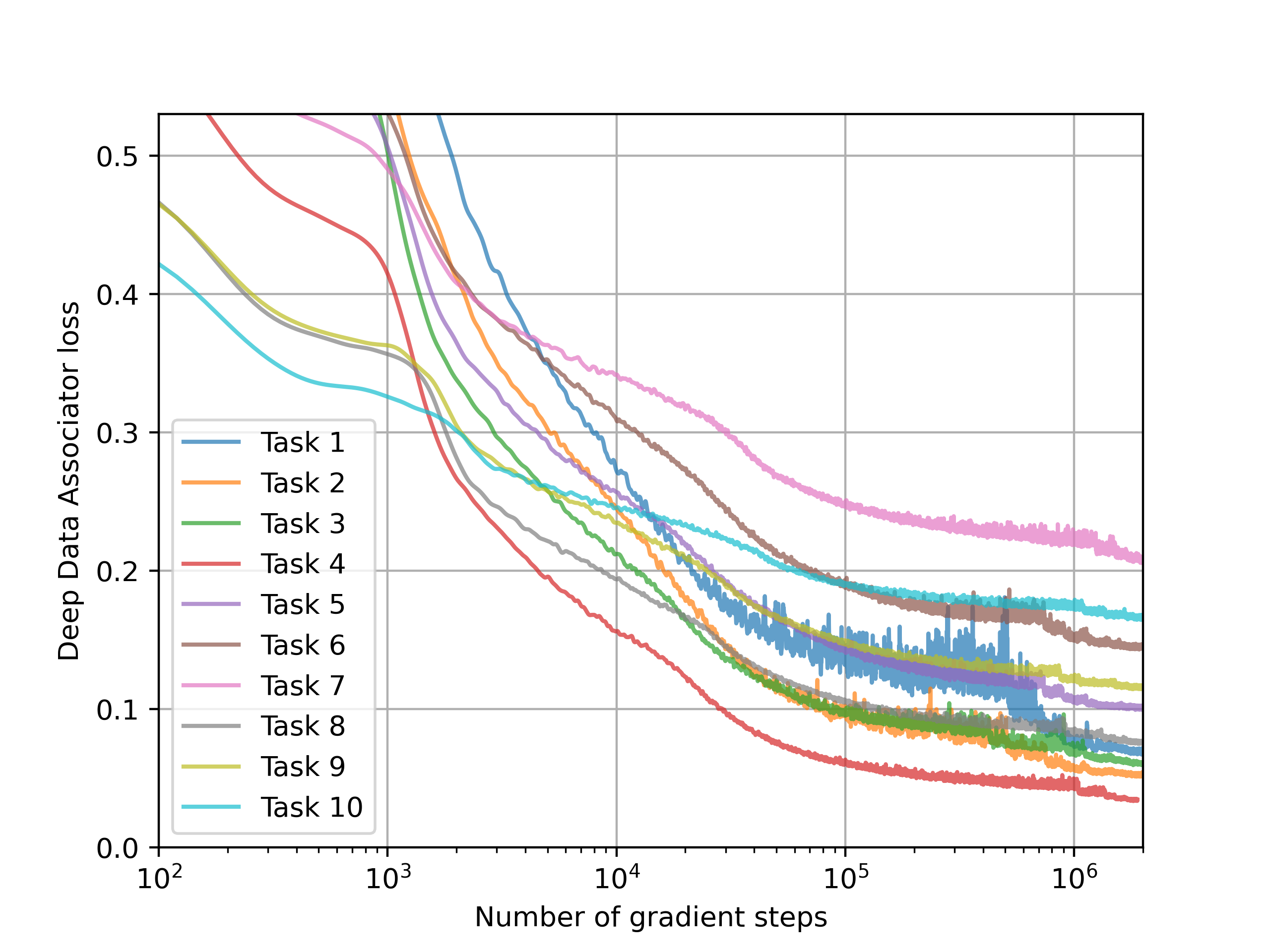
Figure 5: Data association loss $\mathcal{L}_{\text{DDA}}$ during training of the DDA module. Lower values indicate better data association performance.

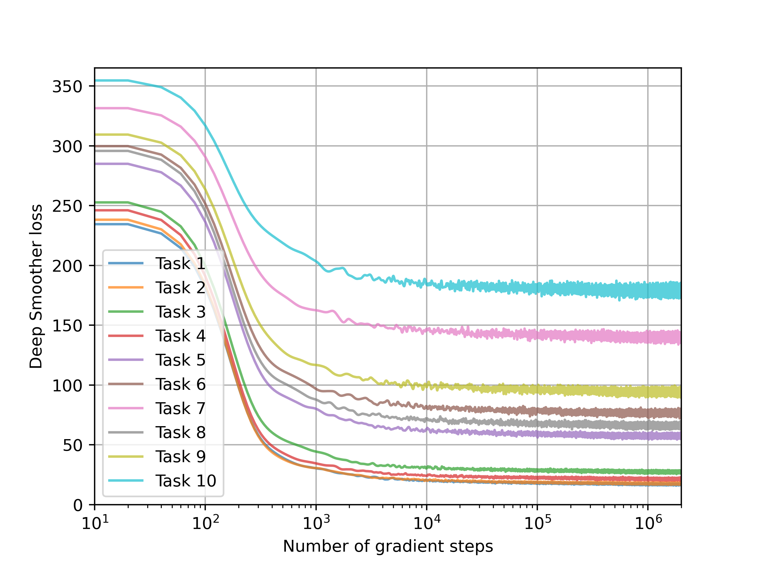
Figure 6: Deep Smoother loss $\mathcal{L}_{\text{DS}}$ values for D3AS in each task vs. number of gradient steps that the DS module was trained for. Lower values indicate better trajectory estimates.

The loss $\mathcal{L}_{\text{DDA}}$ drops sharply at the beginning of the training and starts to slow down for most of the tasks around $10^{5}$ gradient steps. The rate of decrease varies during the optimization, which we believe is due to the model learning different aspects of the task at different points in time. Visual inspection of the model’s output during training showed that it first learns to put almost all the measurements’ mass in the same track. This is due to the fact that, in most tasks, the most prevalent class are false measurements, which makes this a simple way to reduce the loss from a random initialization of the model’s weights. Importantly, the model does not get stuck in this initial state, and a bit later in the training, the DDA slowly starts to try separating true measurements from this track into different tracks, first with easier examples (trajectories with more measurements or in parts of the FOV with fewer false measurements) and later with harder ones.

The sudden decreases close to $10^{6}$ gradient steps are due to the automatic learning rate reduction (see Sec. 5.2.1). This reduction in learning rate is not essential when training the DDA, but in our experiments it improved final performance for all tasks. Furthermore, judging from the shape of the loss curves close to the end of the x-axis, we expect the DDA module to benefit from further training in all tasks, but all trials were restricted to $2\cdot 10^{6}$ gradient steps due to computational limits. We also note that the variance of $\mathcal{L}_{\text{DDA}}$ varies considerably depending on the task. This is most likely due to the different number of measurements in each task. We can interpret the loss defined in (9) as the Monte-Carlo estimate of the expected cross-entropy between $\mathbf{A}$ and $\mathbf{A}^{*}$, where increasing $N$ decreases the variance of this estimate.

Lastly, we observe that $\mathcal{L}_{\text{DDA}}$ is not comparable among tasks with different average number of false measurements, as increasing this number makes it easier for the models to achieve a lower cross-entropy, since most of the measurements will be from the same false measurement class. However, comparing tasks with the same clutter rate – i.e., tasks 3, 5, 6, and 7, or tasks 8, 9, and 10 – shows that indeed increasing measurement or process noise, or decreasing the detection probability makes training harder, and results in worse final data association performance, as expected.

6.2 Training the DS module

Once the DDA module is fully trained, its weights are kept fixed, and then the DS module is trained. The loss curves for this procedure are shown in Fig. 6, where we plot the smoothing loss $\mathcal{L}_{\text{DS}}$, as defined in (14), versus the number of gradient steps taken (in logarithm scale). In contrast to $\mathcal{L}_{\text{DDA}}$, most gains in $\mathcal{L}_{\text{DS}}$ come in the first $10^{4}$ gradient steps, and training beyond $2\cdot 10^{6}$ seems unlikely to yield any additional performance. This, together with the simple sigmoid shape of the loss curves, suggests that optimizing for $\mathcal{L}_{\text{DS}}$ is considerably easier than for $\mathcal{L}_{\text{DDA}}$, which agrees with the intuition that once the data association sub-task is solved, smoothing the individual trajectories is easier.

Furthermore, we note that the ordering of the loss curves is different from the ordering in Fig. 5. The relative challenge in training for each task now depends much less on the clutter rate, and more on the detection probability and measurement/motion noise. For instance, for tasks 1 and 2, which share most of the parameters in Table 1 except the clutter rate, which is doubled for task 2, have very similar loss curves (almost overlapping). This indicates that for these tasks, the DDA module is fairly good at removing false measurements from the DS’s input, effectively making them the same task from the DS’s perspective. On the other hand, more complicated tasks like tasks 7 and 10 have differing loss curves even though they share all parameters but the clutter rate, indicating that the DDA was not able to completely remove the effect of clutter in the DS’s input.

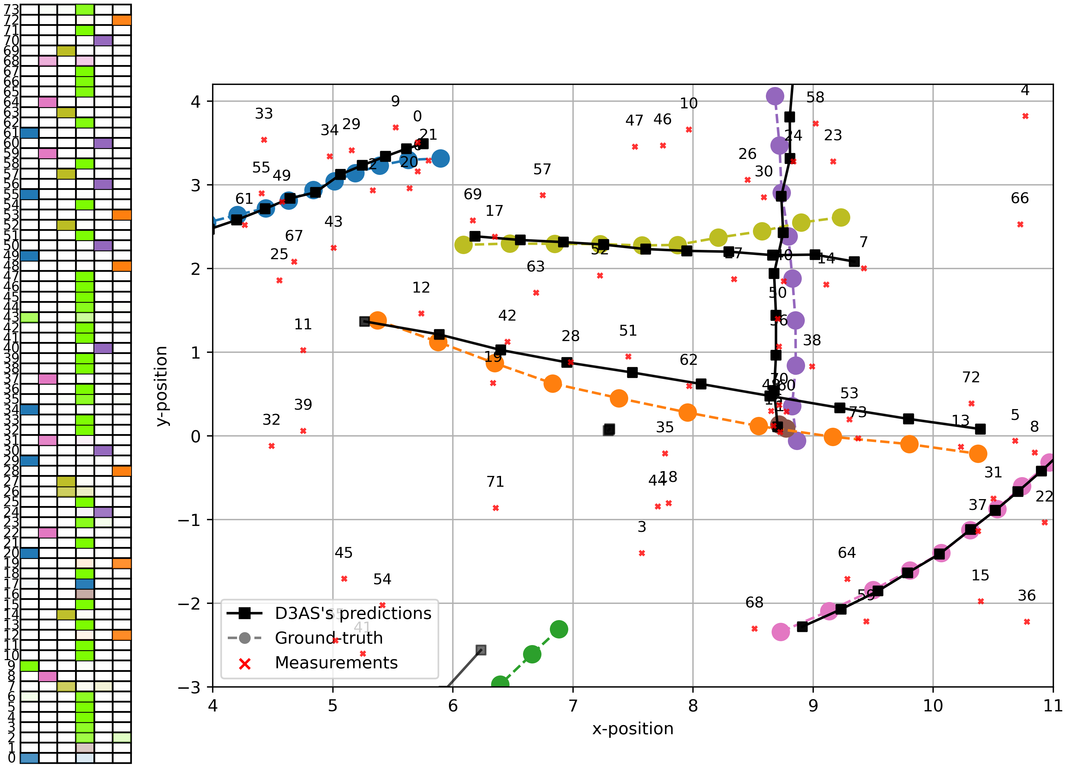
Figure 7: Sample output from D3AS in task 6. Left: data association matrix predicted by the DDA module (tracks with low mass for all measurements are not shown due to limited space). Right: Ground-truth and predicted trajectories by the DS module.

6.3 Visualization of the trained D3AS tracker

After both modules are trained, D3AS is able to leverage all the measurements available to predict reasonable trajectories in all the tasks. A sample output for task 6 is illustrated in Fig. 7. On the left, the data association matrix predicted by the DDA module is shown, and on the right a visualization of the DS’s module output. In the table corresponding to the left, each row corresponds to one measurement, and each column to one track . Each row is color-matched to the object that generated the corresponding measurement, and the transparency in each column depends on how much mass the pmf has in that track. For example, measurement 68 (the 6th row in the table, from top to bottom) has a pmf which has its mode in track number 2 (where the other measurements from this object also have their modes), but also some mass in track number 4 (where most of the false measurements have their modes), signaling that the DDA is uncertain as to whether this is a false measurement.

On the right, in the DS’s output visualization, we show the $xy$ position of all measurements, ground-truth trajectories, and predicted trajectories in the region with $x$ coordinate ranging from 4 to 11 and $y$ from -3 to 4.2 (velocity vectors are not included due to space limitations). All measurements are depicted with a number on top for correspondence with the DA matrix on the left. Ground-truth trajectories have their colors matched to the colors in the DA matrix.

Fig. 7 can give us a glimpse of how hard the tasks are. The only input the algorithms have are the measurements (xy shown as red crosses), and the desired output are the ground-truth trajectories shown. For most ground-truth trajectories, its measurement sequence is considerably noisy, and challenging to tell apart from the false measurements. Nevertheless, the DDA module is able to partition the measurements very well, with only a few true measurements being misclassified as false (measurements 16 and 17) and similarly only a few false measurements misclassified as true (measurements 9 and 43). The DDA module is also able to inform downstream tasks of uncertain associations, for example measurements that have their mode on a certain track but still considerable mass in others (e.g., measurements 19, 26, 68). This is important, for instance, in the smoothing task, where the DS module leverages this uncertainty to decide how much to trust each measurement.

The figure also shows how well the DS module can predict trajectories, given the associations computed by the DDA. Even though measurement noise is high, and the low probability of detection caused many trajectories to not have measurements in multiple time-steps (e.g., the orange trajectory only generated 6 measurements in its 10 time-steps), the DS module is still able to predict reasonable state estimates.

The sample shown in Fig. 7, although hand-picked to illustrate interesting behaviors of both modules compactly, is representative of the tracking quality of D3AS in task 6 and most of the other tasks. The next section provides a thorough evaluation over many samples, and a comparison to TPMBM in all tasks using the TGOSPA metric and the TAA performance measure.

6.4 Comparison to Model-based Bayesian Benchmark

In order to compare D3AS to TPMBM, we compute the average trajectory-GOSPA metric over $10^{3}$ samples from each task. Both algorithms are evaluated on the same samples for fairness and reduced variance, and all samples are drawn from the multi-object models defined in 5 using the task-specific hyperparameters shown in Table 1. The resulting trajectory-GOSPA scores (lower is better) and decompositions for all ten tasks, along with 95% confidence intervals for the means, are displayed in Table 2.

Table 2: Trajectory-GOSPA scores for all tasks.

Task	Alg.	TGOSPA	Loc	Miss	False	Switch
1	D3AS	106.41 ± 3.06	91.11	13.97	1.12	0.21
	TPMBM	117.82 ± 3.47	100.61	16.39	0.64	0.18
2	D3AS	110.54 ± 3.31	90.82	17.81	1.75	0.17
	TPMBM	124.90 ± 3.64	101.02	22.72	0.91	0.25
3	D3AS	154.02 ± 4.30	113.41	38.36	1.74	0.51
	TPMBM	171.12 ± 5.05	111.89	57.23	1.16	0.84
4	D3AS	122.40 ± 3.26	89.67	30.14	2.38	0.21
	TPMBM	152.29 ± 4.64	93.47	57.84	0.77	0.21
5	D3AS	232.27 ± 6.28	150.33	77.90	2.71	1.34
	TPMBM	261.30 $\pm$ 7.63	120.66	138.98	0.30	1.40
6	D3AS	272.17 ± 6.91	163.51	104.11	2.66	1.90
	TPMBM	334.73 $\pm$ 9.21	97.58	235.68	0.12	1.35
7	D3AS	367.31 ± 8.98	204.54	156.18	3.36	3.23
	TPMBM	462.71 $\pm$ 11.73	64.89	396.84	0.00	0.99
8	D3AS	254.13 ± 6.62	146.78	103.43	2.51	1.41
	TPMBM	322.05 $\pm$ 8.99	89.98	230.70	0.24	1.12
9	D3AS	302.53 ± 7.88	157.59	139.28	3.52	2.13
	TPMBM	416.98 ± 11.29	51.15	365.17	0.00	0.67
10	D3AS	418.08 ± 9.53	195.40	216.40	2.66	3.62
	TPMBM	540.06 ± 12.63	15.92	523.88	0.00	0.25

From the table, we can see that both algorithms perform similarly in tasks with low clutter intensity $\lambda_{c}$ and high detection probability $p_{d}$ (tasks 1-3), with D3AS being slightly better in terms of TGOSPA. The low clutter intensity reduces the number of total hypotheses that TPMBM has to keep track of, effectively making it easier for the tracker to estimate the multi-object posterior density. At the same time, the high detection probability decreases the number of hypotheses with non-negligible likelihood within the total hypothesis set, as misdetection associations become unlikely. This, in effect, makes the pruning used by TPMBM to maintain computational tractability not hurt its performance so much, as only a few hypotheses are actually needed to accurately represent the multi-object posterior density.

On the other hand, as we decrease the detection probability and/or increase the clutter intensity, the total number of hypotheses (and the number of these that have non-negligible likelihoods) increases sharply (tasks 4-10). Furthermore, increasing the measurement noise reduces the ability of the model to remove unlikely associations using gating. This increase also exacerbates the impact of the state dependency of the measurement model, making the Gaussian approximations made by TPMBM less accurate. These factors are reflected in a substantial degradation of tracking performance, with a clear trend of worsening as the tasks get more challenging.

In contrast, changing the detection probability and increasing clutter intensity do not have the same impact on the deep learning model, which seems better able to handle the added challenge. As opposed to TPMBM, D3AS does not rely on Gaussian approximations and requires no heuristics; its computational complexity is quadratic on the number of time-steps and independent of the multi-object model’s parameters. Although its TGOSPA performance does decrease as the tasks get more challenging, it does so at a slower rate than TPMBM, leading to an increasing performance gap between these algorithms.

Looking at the TGOSPA decompositions for each task, we observe that in all tasks, D3AS obtains a lower miss rate than TPMBM while not increasing the false rate by a similar amount. This indicates that D3AS is better able to find difficult trajectories than TPMBM, especially in the harder tasks. In fact, for certain samples in task 10, TPMBM was not able to predict any trajectories (all of the Bernoulli components had their existence probabilities below the extraction threshold). Moreover, TPMBM obtained considerably lower localization costs than D3AS for the harder tasks. However, we attribute this to TPMBM’s high missed rate: TGOSPA’s localization costs are only computed for trajectories that the tracker correctly detected, and results are not normalized by the number of detections. Normalizing by the number of detections does not change this, however, as TPMBM focused more on predictions for easier-to-identify trajectories in the harder tasks.

In addition to computing the TGOSPA scores on all tasks, we also analyze the performance in each subtask of data association and smoothing independently. We use the TAA performance measure, as defined in Sec. 5.3.2, to analyze the performance of D3AS and TPMBM in the data association subtask. TPMBM’s data association is extracted from the association histories of each track in the most likely global hypothesis, whereas D3AS’s data association comes directly from the output of the DDA module. The TAA for each task is shown at the top of Table 3 (higher values are better).

Table 3: Top-1 association accuracy and TGOSPA with ground-truth associations for all tasks.

Evaluation	Algorithm	Task 1	Task 2	Task 3	Task 4	Task 5	Task 6	Task 7	Task 8	Task 9	Task 10
Top-1 A.A.	DDA	0.971 ± 0.002	0.965 ± 0.003	0.931 ± 0.004	0.939 ± 0.003	0.867 ± 0.006	0.799 ± 0.007	0.661 ± 0.009	0.811 ± 0.008	0.717 ± 0.008	0.468 ± 0.010
	TPMBM	0.966 ± 0.003	0.951 ± 0.004	0.889 ± 0.006	0.884 ± 0.005	0.765 ± 0.009	0.605 ± 0.011	0.336 ± 0.012	0.617 ± 0.010	0.409 ± 0.011	0.102 ± 0.008
TGOSPA	DS	93.90 ± 2.58	94.84 ± 2.61	120.94 ± 3.17	99.08 ± 2.55	166.94 ± 4.53	180.88 ± 4.56	238.71 ± 6.14	166.44 ± 4.18	180.29 ± 4.87	257.86 ± 6.38
	TPMBM	133.60 ± 3.85	136.16 ± 4.00	172.19 ± 4.85	134.35 ± 3.89	201.17 ± 5.62	210.16 ± 5.55	263.62 ± 6.86	200.91 ± 5.35	204.61 ± 5.70	257.30 ± 6.67

The results show that both algorithms can produce near-perfect data associations for the simpler tasks, but association accuracy drops as the tasks get harder. We see a similar trend in this table, showing that the performance gap between the algorithms increases for harder tasks.

We can also evaluate performance on the smoothing task only. To do so, we feed both algorithms the ground-truth data associations for each measurement, which relieves them from needing to estimate the correct partitions for each track. Hence, all the tracks fed to the algorithms’ smoothing modules only contain the true measurements from ea ch object in the scene. Doing so transforms the MOT task into the single-object setting without any false measurements, effectively evaluating only the smoothing performance of D3AS and TPMBM. We evaluate both methods in this setting using the sum of TGOSPAs between each predicted trajectory and the ground-truth trajectory of its corresponding measurement sequence. The results are shown in the bottom of Table 3 (lower values are better).

Here we see that smoothing performance is superior for the DS module in almost all tasks. Upon closer inspection of individual samples, we found indication that TPMBM can estimate trajectories better than D3AS when they are close to the sensor but becomes considerably worse as trajectories get closer to the edges of the field-of-view (where the measurement model becomes more nonlinear). Among other failure modes, TPMBM incorrectly estimates the start/end times in many of the trajectories, incurring high costs in terms of TGOSPA.

Regarding the performance gap between algorithms, the situation is now different than for the TAA performance measure: as the tasks become more complicated, the performance gap between D3AS and TPMBM decreases. We see two main reasons for this behavior. First, increasing the measurement noise, in specific $\sigma_{r,\text{min}}^{2}$ and $\sigma_{\theta,\text{min}}^{2}$, has the added effect of making the measurement noise covariance $\bm{\Sigma}(\mathbf{x})$ less state-dependent, since $\sigma_{r,\text{max}}^{2}$ and $\sigma_{\theta,\text{max}}$ are kept fixed for all tasks, c.f. (18). Second, when feeding each measurement sequence (partitioned using ground-truth associations) to the DS module, the confidences for each measurement are set to $1$. This essentially evaluates the model under out-of-distribution samples, especially for the harder tasks where the DDA module rarely predicted measurements with high confidences. Ideally, the DS module should be retrained for this setting, but computational limits prevented us from doing so. Nevertheless, we provide these results as they show that in the harder tasks the main advantage of D3AS is being able to perform data association better, therefore validating the efficacy of the DDA module.

References

- [1] Y.-C. Yoon, D. Y. Kim, Y.-M. Song, K. Yoon, and M. Jeon, “Online multiple pedestrians tracking using deep temporal appearance matching association,” Information Sciences, vol. 561, pp. 326–351, 2021.
- [2] A. Rangesh and M. M. Trivedi, “No blind spots: Full-surround multi-object tracking for autonomous vehicles using cameras and lidars,” IEEE Transactions on Intelligent Vehicles, vol. 4, no. 4, pp. 588–599, 2019.
- [3] P. Nillius, J. Sullivan, and S. Carlsson, “Multi-target tracking-linking identities using bayesian network inference,” in 2006 IEEE Computer Society Conference on Computer Vision and Pattern Recognition (CVPR’06), vol. 2. IEEE, 2006, pp. 2187–2194.
- [4] C. J. Harris, A. Bailey, and T. Dodd, “Multi-sensor data fusion in defence and aerospace,” The Aeronautical Journal (1968), vol. 102, no. 1015, p. 229–244, 1998.
- [5] E. Itskovits, A. Levine, E. Cohen, and A. Zaslaver, “A multi-animal tracker for studying complex behaviors,” BMC Biology, vol. 15, no. 1, p. 29, Apr 2017.
- [6] C. Spampinato, Y.-H. Chen-Burger, G. Nadarajan, and R. B. Fisher, “Detecting, tracking and counting fish in low quality unconstrained underwater videos.” VISAPP (2), vol. 2008, no. 514-519, p. 1, 2008.
- [7] R. P. S. Mahler, Statistical Multisource-Multitarget Information Fusion. USA: Artech House, Inc., 2007.
- [8] A. C. Harvey, “Forecasting, structural time series models and the kalman filter,” 1990.
- [9] Á. F. García-Fernández and L. Svensson, “Trajectory phd and cphd filters,” IEEE Transactions on Signal Processing, vol. 67, no. 22, pp. 5702–5714, 2019.
- [10] B.-N. Vo and B.-T. Vo, “A multi-scan labeled random finite set model for multi-object state estimation,” IEEE Transactions on signal processing, vol. 67, no. 19, pp. 4948–4963, 2019.
- [11] Y. Xia, K. Granström, L. Svensson, Á. F. García-Fernández, and J. L. Williams, “Multi-scan implementation of the trajectory poisson multi-bernoulli mixture filter,” Journal of Advances in Information Fusion, vol. 14, no. 2, pp. 213–235, 2019.
- [12] K. Granström, L. Svensson, Y. Xia, J. Williams, and Á. F. García-Femández, “Poisson multi-Bernoulli mixture trackers: Continuity through random finite sets of trajectories,” in 2018 21st International Conference on Information Fusion (FUSION). IEEE, 2018, pp. 1–5.
- [13] K. Granström, L. Svensson, Y. Xia, J. Williams, and Á. F. García-Fernández, “Poisson multi-Bernoulli mixtures for sets of trajectories,” arXiv preprint arXiv:1912.08718, 2019.
- [14] S. Särkkä, Bayesian filtering and smoothing. Cambridge University Press, 2013, no. 3.
- [15] Z. Dai, H. Liu, Q. V. Le, and M. Tan, “Coatnet: Marrying convolution and attention for all data sizes,” Advances in Neural Information Processing Systems, vol. 34, pp. 3965–3977, 2021.
- [16] Q. Wang, B. Li, T. Xiao, J. Zhu, C. Li, D. F. Wong, and L. S. Chao, “Learning deep transformer models for machine translation,” in ACL (1). Association for Computational Linguistics, 2019, pp. 1810–1822.
- [17] D. Silver, T. Hubert, J. Schrittwieser, I. Antonoglou, M. Lai, A. Guez, M. Lanctot, L. Sifre, D. Kumaran, T. Graepel et al., “A general reinforcement learning algorithm that masters chess, shogi, and Go through self-play,” Science, vol. 362, no. 6419, pp. 1140–1144, 2018.
- [18] A. Ramesh, P. Dhariwal, A. Nichol, C. Chu, and M. Chen, “Hierarchical text-conditional image generation with CLIP latents,” CoRR, vol. abs/2204.06125, 2022.
- [19] P. Dendorfer, A. Osep, A. Milan, K. Schindler, D. Cremers, I. Reid, S. Roth, and L. Leal-Taixé, “MOTchallenge: A benchmark for single-camera multiple target tracking,” International Journal of Computer Vision, pp. 1–37, 2020.
- [20] G. Ciaparrone, F. L. Sánchez, S. Tabik, L. Troiano, R. Tagliaferri, and F. Herrera, “Deep learning in video multi-object tracking: A survey,” Neurocomputing, vol. 381, pp. 61–88, 2020.
- [21] Y. Xu, X. Zhou, S. Chen, and F. Li, “Deep learning for multiple object tracking: a survey,” IET Computer Vision, vol. 13, no. 4, pp. 355–368, 2019.
- [22] C.-Y. Chong, “An overview of machine learning methods for multiple target tracking,” in 2021 IEEE 24th International Conference on Information Fusion (FUSION), 2021, pp. 1–9.
- [23] J. Chen, H. Sheng, Y. Zhang, and Z. Xiong, “Enhancing detection model for multiple hypothesis tracking,” in Proceedings of the IEEE Conference on Computer Vision and Pattern Recognition Workshops, 2017, pp. 18–27.
- [24] A. Milan, S. H. Rezatofighi, A. Dick, I. Reid, and K. Schindler, “Online multi-target tracking using recurrent neural networks,” in Thirty-First AAAI Conference on Artificial Intelligence, 2017.
- [25] H. Zhou, W. Ouyang, J. Cheng, X. Wang, and H. Li, “Deep continuous conditional random fields with asymmetric inter-object constraints for online multi-object tracking,” IEEE Transactions on Circuits and Systems for Video Technology, vol. 29, no. 4, pp. 1011–1022, 2018.
- [26] P. Bergmann, T. Meinhardt, and L. Leal-Taixe, “Tracking without bells and whistles,” in Proceedings of the IEEE/CVF International Conference on Computer Vision, 2019, pp. 941–951.
- [27] S. Sun, N. Akhtar, X. Song, H. Song, A. Mian, and M. Shah, “Simultaneous detection and tracking with motion modelling for multiple object tracking,” in European Conference on Computer Vision. Springer, 2020, pp. 626–643.
- [28] S. Sun, N. Akhtar, H. Song, A. Mian, and M. Shah, “Deep affinity network for multiple object tracking,” IEEE Transactions on Pattern Analysis and Machine Intelligence, vol. 43, no. 1, pp. 104–119, 2019.
- [29] B. Pang, Y. Li, Y. Zhang, M. Li, and C. Lu, “Tubetk: Adopting tubes to track multi-object in a one-step training model,” in Proceedings of the IEEE/CVF Conference on Computer Vision and Pattern Recognition, 2020, pp. 6308–6318.
- [30] Y. Zhang, C. Wang, X. Wang, W. Zeng, and W. Liu, “Fairmot: On the fairness of detection and re-identification in multiple object tracking,” International Journal of Computer Vision, pp. 1–19, 2021.
- [31] P. Voigtlaender, M. Krause, A. Osep, J. Luiten, B. B. G. Sekar, A. Geiger, and B. Leibe, “MOTS: Multi-object tracking and segmentation,” in Proceedings of the IEEE/CVF Conference on Computer Vision and Pattern Recognition, June 2019.
- [32] X. Weng, Y. Wang, Y. Man, and K. M. Kitani, “Gnn3dmot: Graph neural network for 3d multi-object tracking with 2d-3d multi-feature learning,” in Proceedings of the IEEE/CVF Conference on Computer Vision and Pattern Recognition, 2020, pp. 6499–6508.
- [33] G. Brasó and L. Leal-Taixé, “Learning a neural solver for multiple object tracking,” in Proceedings of the IEEE/CVF Conference on Computer Vision and Pattern Recognition, 2020, pp. 6247–6257.
- [34] J. Li, X. Gao, and T. Jiang, “Graph networks for multiple object tracking,” in Proceedings of the IEEE/CVF Winter Conference on Applications of Computer Vision, 2020, pp. 719–728.
- [35] T. Meinhardt, A. Kirillov, L. Leal-Taixe, and C. Feichtenhofer, “Trackformer: Multi-object tracking with transformers,” in Proceedings of the IEEE/CVF Conference on Computer Vision and Pattern Recognition, 2022, pp. 8844–8854.
- [36] F. Zeng, B. Dong, Y. Zhang, T. Wang, X. Zhang, and Y. Wei, “Motr: End-to-end multiple-object tracking with transformer,” in European Conference on Computer Vision (ECCV), 2022.
- [37] P. Chu, J. Wang, Q. You, H. Ling, and Z. Liu, “TransMOT: Spatial-temporal graph transformer for multiple object tracking,” arXiv preprint arXiv:2104.00194, 2021.
- [38] P. Sun, Y. Jiang, R. Zhang, E. Xie, J. Cao, X. Hu, T. Kong, Z. Yuan, C. Wang, and P. Luo, “Transtrack: Multiple-object tracking with transformer,” arXiv preprint arXiv:2012.15460, 2020.
- [39] J. Cai, M. Xu, W. Li, Y. Xiong, W. Xia, Z. Tu, and S. Soatto, “Memot: Multi-object tracking with memory,” in Proceedings of the IEEE/CVF Conference on Computer Vision and Pattern Recognition (CVPR), June 2022, pp. 8090–8100.
- [40] Y. Liu, T. Bai, Y. Tian, Y. Wang, J. Wang, X. Wang, and F.-Y. Wang, “Segdq: Segmentation assisted multi-object tracking with dynamic query-based transformers,” Neurocomputing, vol. 481, pp. 91–101, 2022.
- [41] J. Pinto, G. Hess, W. Ljungbergh, Y. Xia, L. Svensson, and H. Wymeersch, “Next generation multitarget trackers: Random finite set methods vs transformer-based deep learning,” in 24th International Conference on Information Fusion (FUSION). IEEE, 2021, pp. 1–8.
- [42] A. Vaswani, N. Shazeer, N. Parmar, J. Uszkoreit, L. Jones, A. N. Gomez, Ł. Kaiser, and I. Polosukhin, “Attention is all you need,” Advances in Neural Information Processing Systems, vol. 30, pp. 5998–6008, 2017.
- [43] J. Devlin, M. Chang, K. Lee, and K. Toutanova, “BERT: pre-training of deep bidirectional transformers for language understanding,” in NAACL-HLT (1). Association for Computational Linguistics, 2019, pp. 4171–4186.
- [44] R. P. Mahler, Advances in statistical multisource-multitarget information fusion. Artech House, 2014.
- [45] N. Carion, F. Massa, G. Synnaeve, N. Usunier, A. Kirillov, and S. Zagoruyko, “End-to-end object detection with transformers,” in European Conference on Computer Vision, vol. 12346. Springer, 2020, pp. 213–229.
- [46] L. J. Ba, J. R. Kiros, and G. E. Hinton, “Layer normalization,” in Neural Information Processing Systems Deep Learning Symposium, 2016.
- [47] Z. Sun, S. Cao, Y. Yang, and K. M. Kitani, “Rethinking transformer-based set prediction for object detection,” in Proceedings of the IEEE/CVF international conference on computer vision, 2021, pp. 3611–3620.
- [48] F. Li, H. Zhang, S. Liu, J. Guo, L. M. Ni, and L. Zhang, “Dn-detr: Accelerate detr training by introducing query denoising,” in Proceedings of the IEEE/CVF Conference on Computer Vision and Pattern Recognition, 2022, pp. 13 619–13 627.
- [49] H. Zhang, F. Li, S. Liu, L. Zhang, H. Su, J. Zhu, L. M. Ni, and H.-Y. Shum, “Dino: Detr with improved denoising anchor boxes for end-to-end object detection,” arXiv preprint arXiv:2203.03605, 2022.
- [50] S. Liu, F. Li, H. Zhang, X. Yang, X. Qi, H. Su, J. Zhu, and L. Zhang, “DAB-DETR: dynamic anchor boxes are better queries for DETR,” in International Conference on Learning Representations (Poster), 2022.
- [51] X. Zhu, W. Su, L. Lu, B. Li, X. Wang, and J. Dai, “Deformable DETR: Deformable transformers for end-to-end object detection,” in International Conference on Learning Representations, 2021.
- [52] J. Pinto, Y. Xia, L. Svensson, and H. Wymeersch, “An uncertainty-aware performance measure for multi-object tracking,” IEEE Signal Processing Letters, vol. 28, no. 1689–1693, 2021.
- [53] I. Loshchilov and F. Hutter, “Decoupled weight decay regularization,” in International Conference on Learning Representations (Poster), 2019.
- [54] D. F. Crouse, “On implementing 2D rectangular assignment algorithms,” IEEE Transactions on Aerospace and Electronic Systems, vol. 52, no. 4, pp. 1679–1696, 2016.
- [55] Á. F. García-Fernández, L. Svensson, J. L. Williams, Y. Xia, and K. Granström, “Trajectory Poisson multi-Bernoulli filters,” IEEE Transactions on Signal Processing, vol. 68, pp. 4933–4945, 2020.
- [56] Á. F. García-Fernández, L. Svensson, M. R. Morelande, and S. Särkkä, “Posterior linearization filter: Principles and implementation using sigma points,” IEEE Transactions on Signal Processing, vol. 63, no. 20, pp. 5561–5573, 2015.
- [57] Á. F. García-Fernández, J. Ralph, P. Horridge, and S. Maskell, “A Gaussian filtering method for multitarget tracking with nonlinear/non-Gaussian measurements,” IEEE Transactions on Aerospace and Electronic Systems, vol. 57, no. 5, pp. 3539–3548, 2021.
- [58] I. Arasaratnam and S. Haykin, “Cubature kalman filters,” IEEE Transactions on Automatic Control, vol. 54, no. 6, pp. 1254–1269, 2009.
- [59] D. Crouse, “Basic tracking using nonlinear 3D monostatic and bistatic measurements,” IEEE Aerospace and Electronic Systems Magazine, vol. 29, no. 8, pp. 4–53, 2014.
- [60] Á. F. García-Fernández, A. S. Rahmathullah, and L. Svensson, “A metric on the space of finite sets of trajectories for evaluation of multi-target tracking algorithms,” IEEE Trans. Signal Process., vol. 68, pp. 3917–3928, 2020.
- [61] A. S. Rahmathullah, Á. F. García-Fernández, and L. Svensson, “Generalized optimal sub-pattern assignment metric,” in IEEE International Conference on Information Fusion (Fusion), 2017.