Dark matter freeze-in from non-equilibrium QFT: towards a consistent treatment of thermal effects

Abstract

We study thermal corrections to a model of real scalar dark matter interacting feebly with a SM fermion and a gauge-charged vector-like fermion. We employ the Closed-Time-Path (CTP) formalism for our calculation and go beyond previous works by including the full dependence on the relevant mass scales as opposed to using (non)relativistic approximations. In particular, we use 1PI-resummed propagators without relying on the Hard-Thermal-Loop approximation. We conduct our analysis at leading order in the loop expansion of the 2PI effective action and compare our findings to commonly used approximation schemes, including the aforementioned Hard-Thermal-Loop approximation and results obtained from solving Boltzmann equations using thermal masses as a regulator for $t$-channel divergences. We find that the Boltzmann approach deviates between $-10\%$ and $+30\%$ from our calculation, where the size and sign strongly depends on the mass splitting between the DM candidate and the gauge-charged parent. The HTL-approximated result is more precise for small gauge couplings and is percent level accurate for large mass splittings, whereas it overestimates the relic density up to $25\%$ for small mass splittings. Tree-level propagators lead to underabundant DM as they do not account for scattering contributions and can deviate up to $-100\%$ from the 1PI-resummed result.

1 Introduction

One of the most puzzling questions of physics is the origin and nature of Dark Matter (DM), a non-luminous, gravitationally interacting, and (preferably) non-relativistic substance permeating the Universe at every cosmological scale [1, 2]. If DM has a particle nature, it cannot be accommodated in the Standard Model (SM) of particle physics so that new physics beyond the Standard Model (BSM) needs to be involved. Among the various possibilities, one of the most studied scenarios is that of weakly interacting massive particles (WIMPs) in thermal equilibrium with the primordial thermal bath of SM species. As the temperature of the plasma decreases with the expanding Universe, the DM particles follow their equilibrium abundance until temperatures of order their mass, after which they thermally decouple because their interactions stop being efficient enough to keep them in chemical equilibrium. Eventually, these interactions effectively switch off and the DM abundance departs from its equilibrium value at temperatures smaller than the DM mass, $T\simeq M/25$, so that the DM particles are non-relativistic and thermal corrections are not expected to be very large. After this moment, the DM comoving number density freezes to a value that remains constant during the subsequent cosmic epochs. This is the well-known freeze-out mechanism.

One of the main advantages of this paradigm is that thermal equilibrium erases any information regarding the initial conditions prior to freeze-out so that one does not need to specify them and the DM relic abundance is completely set by couplings and masses of the particles involved in the production reactions. Moreover, WIMPs are phenomenologically motivated by the appealing abundance of potential signatures, ranging from production at colliders to direct detection of their collisions in terrestrial detectors and indirect detection with telescopes of the byproducts of their annihilations within and nearby the Galaxy. However, the lack of signatures relatable to such particles has put the vanilla WIMP paradigm into a corner [3, 4]. Even though this could be due to a less-trivial structure of the dark sector, perhaps involving a mass-compressed spectrum [5, 6], another possibility is that DM features very small interactions with the visible sector, rendering its detection more challenging.

This is the case for DM being a feebly interacting massive particle (FIMP) produced via the freeze-in mechanism [7, 8, 9]. In this framework, DM is assumed to have been created in the early universe from a negligible initial abundance via $1~{}\rightarrow~{}2$ decays or $2~{}\rightarrow~{}2$ annihilations possibly involving heavier dark mediators and SM particles. The crucial assumption is that DM interacts with these particles through very small couplings, in such a way that it can never reach thermal equilibrium. As a consequence, contrary to freeze-out, backreactions are negligible and the comoving number density of FIMP DM grows from zero until it freezes-in to the present-day value around $T\sim M$, when its production rate becomes inefficient in comparison to the expansion rate of the Universe. This means that the production dynamics are sensitive to the high-temperature regime in which DM is relativistic. In this regime, if the dark mediators are part of the thermal plasma, their physical properties get corrected by finite-temperature effects and, in return, the production of DM is also affected. This is in contrast to freeze-out, where the production dynamics peak in the non-relativistic regime.

Such corrections have recently received major attention. Firstly, accounting for the full relativistic quantum statistics (Fermi-Dirac or Bose-Einstein) in the freeze-in collision operators instead of Maxwell-Boltzmann distributions can lead up to $\mathcal{O}(10\%)$ differences in the DM abundance [10, 11, 12, 13]. Secondly, thermal corrections in the form of thermal masses have been included in decay and scattering processes in order to regulate infrared divergences affecting $t$-channel diagrams involving massless states. Depending on the model considered, thermal masses open up a broader range of kinematically-allowed regimes, allowing for decay and inverse decay processes that would be forbidden at zero temperature, and, moreover, they make the solution of the Boltzmann equation infrared-finite (see, for example, Refs. [14, 15, 16, 12, 17, 18, 13, 19]).

Despite the inclusion of relativistic statistics and thermal masses, the previous works relied on semi-classical Boltzmann approach, where production rates originate from integrating a cross-section with thermal masses added as an ad-hoc correction. The cross-section itself is derived from an in-out S-matrix element for asymptotically-free states. However, in medium, the concept of free particles and asymptotic states breaks down. Here, a consistent treatment of finite-density effects is necessary, requiring a full quantum-field-theoretical approach at finite-temperature [20, 21], going beyond the simple addition of thermal masses. This can be done essentially in two ways, namely within the imaginary-time (or Matsubara) formalism [22, 21, 23], which only applies in thermal equilibrium, and within the real-time (also known as closed-time-path, or Keldysh-Schwinger) formalism [24, 25, 26, 27, 28, 29, 30, 31, 32, 33, 34, 35, 36]. This is also the standard theoretical framework to study non-equilibrium processes [37, 38].

Recently, a major step towards a consistent treatment of DM freeze-in at finite temperature that does not rely on the semi-empirical Boltzmann approach has been taken by Ref. [39], where the authors rely on the imaginary-time formalism to compute the production rate of Majorana DM fermion particles from three-body and four-body reactions involving a heavier gauge charged scalar mediator and a SM fermion in thermal equilibrium (for related results in the freeze-out context see also [40, 41]). The rates are computed in the ultrarelativistic regime by exploiting the large momentum limit of the hard thermal loop (HTL) resummed propagators of the equilibrated fields [42, 43, 44] and by adding on top reactions enhanced by multiple soft scatterings with the plasma, efficient at high temperatures. Such quantum phenomenon, named the Landau-Pomeranchuk-Migdal (LPM) effect [45, 46], is calculated for massless particles and switched off by a phenomenological prescription in the non-relativistic regime $T\ll M$, where the Born rate is assumed to hold. Such an interpolation allows the characterization of particle production in every temperature regime, although relying on a high-temperature approximation of the production rate around the bulk of freeze-in production ($T\sim M$). Even though improved interpolations between LPM and Born rates are possible [47], whether accounting for a massive mediator and DM candidate would sensibly change the production rate is an open question due to the highly complex calculations needed to correctly and smoothly switch from one regime to another.

In our work, we choose to follow a different and complementary approach. It relies on deriving the evolution of the DM abundance from quantum kinetic Kadanoff-Baym equations (see [48]) in the Closed-Time-Path (CTP) formalism of non-equilibrium quantum field theory. This corresponds to following the time evolution of two-point correlators defined on a complex time contour via Schwinger-Dyson equations derived as the stationary points of a two-particle-irreducible (2PI) effective action [26, 27, 37, 49, 50, 38]. There are several advantages to this method. First, the CTP is constructed to track the temporal evolution of expectation values of $n$-point correlation functions in a fully-interacting background, in contrast to the S-matrix formalism employed in the semi-classical Boltzmann approach (in fact, it is also called in-in formalism, in opposition to in-out). Moreover, since the expectation values of two-point functions are directly related to statistical properties of fields, the CTP formalism is well-suited to describe particle production in the early Universe and the evolution equations for the correlators can be turned into rate equations for particle number densities. Additionally, 2PI effective actions provide a framework that can systematically account for quantum and thermal corrections by resumming a much larger set of diagrams with respect to more standard 1PI approaches, better probing the field configuration space. The here chosen formalism has been extensively employed in the context of leptogenesis [51, 52, 53, 54, 55, 56, 57, 58, 59, 60, 61, 62, 63, 64, 65, 66, 67, 68, 69, 70, 71, 72, 73, 74, 75, 76, 77, 78], with fewer concrete applications to DM models [79, 80, 81, 82].

To set ourselves in a concrete context, we choose a model where DM is a real scalar singlet, interacting with a SM-charged heavy dark sector vectorlike fermion and a SM fermion via a feeble Yukawa coupling. The two fermions are kept in thermal equilibrium by their gauge interactions. This model has also been considered in freeze-out [83, 84, 85, 86, 87] and freeze-in contexts [18, 88]. In the CTP formalism, the evolution equation for the DM number density is governed by an interaction rate which, in resemblance of the optical theorem, is given by the integral of the imaginary part of the DM retarded self-energy. The DM self-energy can be derived from functional differentiation of the 2PI effective action and is given at leading order (LO) by a loop of dark and SM fermion propagators. Since these propagators come also from the 2PI effective action, they are formally exact and correspond to the solution of an infinite hierarchical tower of coupled Schwinger-Dyson equations. In practice, such hierarchy needs to be truncated. The resulting propagators resum an infinite series of one-loop self-energy insertions, which, in our case, correspond to loop corrections coming from interactions with gauge bosons in the thermal bath. Thus, the resummed propagators encode the information about the interactions of the two fermions with the thermal plasma and they contain the finite-temperature corrections to their physical properties, such as their dispersion relations and damping rates [20]. In principle, next-to-leading order (NLO) contributions coming from two-loop corrections to the DM self-energy can be relevant in certain kinematic regimes. For example, the aforementioned LPM effect can be captured by resumming an infinite series of 2PI “ladder” diagrams featuring gauge boson insertions between the two fermion propagators in the DM self-energy loop. However, in this work, we will omit such terms, both because of the aforementioned theoretical uncertainties and complexities when several mass scales are involved beside the temperature, and because an implementation that would more appropriately align with the formalism here considered should rely on equations of motion derived from 3PI effective actions, including those for proper vertices [49]. Nevertheless, we will comment on the omitted effect and we will provide with an estimate on its impact based on existing literature, while we plan to address it in a follow-up work.

With this ingredients at hand, we calculate the DM interaction rate accounting for the one-loop resummed propagators, including the mediator and DM in-vacuum masses beyond the HTL approximation and we integrate it over time to obtain the DM relic density. We then compare such results with the DM abundances obtained using the conventional Boltzmann equation approach, accounting for decays with in-vacuum masses only, by including thermal masses, and by further including scattering processes with thermal mass regulated propagators. Finally, we confront the same calculation when performed with HTL propagators as well as with their tree-level (large momentum) limit. To summarize our results, we find that the accuracy of each method strongly depends on the mass splitting of the two vacuum mass scales involved. More specifically:

• The relic density obtained from a Boltzmann approach considering only decay contributions fails to accurately describe the DM production. Especially for small mass splittings, the relic density can be underestimated by up to $100\%$ with respect to the CTP result with one-loop resummed propagators. Remarkably, the inclusion of thermal masses worsens the accuracy of the result when only decays are considered.

• Adding DM production from scatterings with propagators regulated by thermal masses can accidentally cancel the overestimated production from decays, deviating from $-10\%$ to $+30\%$ when increasing the mass splitting. The discrepancies can be cut in half when considering the appropriate equilibrium distribution functions instead of Boltzmann statistics, which soften DM production because of the Pauli blocking associated with the accompanying final state fermion. The accuracy of this method only mildly depends on the effective gauge coupling of the parent particle.

• the HTL-approximated propagators lead to percent-level accurate results with respect to one-loop resummed propagators, as long as the two vacuum mass scales are well separated. For smaller mass splittings, however, they can overestimate the relic density by roughly $25\%$. Additionally, the size of this deviation grows with larger effective gauge couplings of the interacting fermions.

The paper is organized as follows: In Sec. 2, we introduce the example DM model set-up and we briefly review the conventional freeze-in production mechanism with a semi-classical Boltzmann equation approach. In Sec. 3, we first recall some elements of the closed-time-path (CTP) formalism and we show how the rate equations for DM are obtained (we refer to Appendices A, B for a more detailed discussion). Then, we derive the DM production rates in the three levels of approximation for the fermion propagators. In Sec. 4, we present the results of our analysis and discuss the deviations of each method from the relic abundance obtained with one-loop resummed propagators. Finally, we conclude in Sec. 5.

2 Example model set-up and semi-classical Boltzmann approach

In this section, we introduce the class of freeze-in models that will serve as illustrative examples to study the impact of a more accurate treatment of finite-temperature effects. Furthermore, we will sketch the calculation of the relic density for freeze-in DM in the well-established semi-classical Boltzmann approach.

2.1 Vectorlike portal FIMP models

We will focus on a concrete class of models where DM is a gauge-singlet scalar field $s$ featuring a Yukawa interaction with a heavier vectorlike fermion $F$ (which will be referred to as the “mediator”) and a SM fermion $f$. This model has been sometimes named vectorlike portal and has been already considered in the freeze-out [83, 84, 85, 87] and freeze-in contexts [18, 86, 88] without thermal effects. Its Lagrangian density reads as

$$\mathcal{L}=\mathcal{L}_{\text{SM}}+\frac{1}{2}(\partial_{\mu}s)^{2}-\frac{1}{2}m_{s}^{2}s^{2}-V(s,H)+\bar{F}\left(i\not{D}-m_{F}\right)F-\left[y_{\text{DM}}\bar{F}fs+h.c.\right]\,,$$ (2.1)

where $V(s,H)$ is the scalar potential of the DM including its possible interaction with the Higgs field, $D_{\mu}$ is the covariant derivative, and $y_{\text{DM}}$ is the portal Yukawa coupling. Since we want to focus on the freeze-in regime, this coupling is supposed to be $y_{\text{DM}}\ll 1$. The mediator and the DM scalar are stabilized by a $Z_{2}$ symmetry under which they are odd, while the SM fields remain even. This allows DM to be the lightest stable dark sector particle.

In this work, we will not consider the influence of DM self-interactions and of the interaction terms with the Higgs in the scalar potential. This allows us to focus on a reduced set of parameters, namely the gauge couplings, the Yukawa coupling $y_{\text{DM}}$, and the masses $m_{s}=m_{\text{DM}}$ and $m_{F}$. In particular, we require the self-coupling and the coupling to the Higgs to be sufficiently small in order not to equilibrate the scalar singlet with itself or with the SM bath (see, e.g., Refs. [89, 90, 86, 13]).

To preserve gauge invariance, the heavy mediators $F$ must belong to the same representation of the SM gauge groups as the SM fermion $f$ they interact with, and hence they are also gauge charged. With SM fermions coming in five different representations, there are as many realizations of the model. In this work we parametrize the gauge interaction of the vectorlike fermion $F$ and the the SM $f$ via an effective gauge coupling $G$ given by

$$G=Y^{2}g_{1}^{2}+C_{2}\left(\mathcal{R}_{2}\right)g_{2}^{2}+C_{2}\left(\mathcal{R}_{3}\right)g_{3}^{2}\,,$$ (2.2)

where $g_{1}$, $g_{2}$ and $g_{3}$ are the SM gauge couplings for $U(1)_{Y}$, $SU(2)_{L}$ and $SU(3)_{C}$, respectively, $Y$ is the weak hypercharge of $f/F$, while $\mathcal{R}_{2}$ and $\mathcal{R}_{3}$ are the corresponding representations under $SU(2)_{L}$ and $SU(3)_{C}$, whose Casimir invariants are denoted as $C_{2}({\cal R_{X}})$. We state some typical values for the effective gauge coupling $G$ for the five different realizations of this model in Table 1.

	$Y$	$SU(2)$	$SU(3)$	$G$	$\mu=M_{Z}$	$10^{4}\,\text{GeV}$	$10^{7}\,\text{GeV}$	$10^{10}\,\text{GeV}$
$e_{L}$	$-1/2$	$\mathbf{2}$	$\mathbf{1}$	$\dfrac{g_{1}^{2}}{4}+\dfrac{3g_{2}^{2}}{4}$	0.38	0.4	0.46	0.52
$q_{L}$	$+1/6$	$\mathbf{2}$	$\mathbf{3}$	$\dfrac{g_{1}^{2}}{36}+\dfrac{3g_{2}^{2}}{4}+\dfrac{4g_{3}^{2}}{3}$	2.3	1.6	1.2	1.0
$e_{R}$	$-1$	$\mathbf{1}$	$\mathbf{1}$	$g_{1}^{2}$	0.21	0.22	0.24	0.26
$u_{R}$	$+2/3$	$\mathbf{1}$	$\mathbf{3}$	$\dfrac{4g_{1}^{2}}{9}+\dfrac{4g_{3}^{2}}{3}$	2.1	1.3	0.9	0.7
$d_{R}$	$-1/3$	$\mathbf{1}$	$\mathbf{3}$	$\dfrac{g_{1}^{2}}{9}+\dfrac{4g_{3}^{2}}{3}$	2.0	1.2	0.8	0.6

Table 1: The effective gauge coupling $G$ (cf. Eq.(2.2)) in various models, classified according to the gauge quantum numbers of the SM fermion and the BSM vectorlike fermion involved. We use the 1-loop beta functions of the SM gauge couplings to evaluate $G$ at several renormalization scales $\mu$ encompassing some of the values of $G$ considered in this work.

The gauge interactions are sufficiently large to safely assume that the mediators, as well as the SM fermions, interact quickly enough with the thermal bath to reach a state of thermal equilibrium so that we do not need to study their kinetic evolution. Furthermore, we parametrize the mass splitting in the dark sector by the dimensionless variable

$$\delta=\frac{m_{F}-m_{\text{DM}}}{m_{F}}\,.$$ (2.3)

With these definitions, the four parameters of our model class are the portal Yukawa $y_{\text{DM}}$, the effective gauge coupling $G$, the mass splitting in the dark sector $\delta$ and the parent particle mass $m_{F}$.

2.2 Semi-classical Boltzmann approach

In this section, we summarize the most standard treatment of freeze-in production of DM in the context of the semi-classical Boltzmann equations, to which we will later compare our work. The evolution of the DM number density $n_{\text{DM}}$ is given by

$$\dot{n}_{\text{DM}}+3Hn_{\text{DM}}=\sum_{\text{processes}}\gamma^{\text{eq}}_{\mathrm{DM}}\left(\mathcal{I}\rightarrow\mathcal{F}\right)\left(\prod_{i\in\mathcal{I}}\frac{n_{i}}{n_{i}^{\text{eq}}}-\prod_{f\in\mathcal{F}}\frac{n_{f}}{n_{f}^{\text{eq}}}\right)\equiv\gamma_{\text{DM}}\,,$$ (2.4)

with

$$\gamma^{\text{eq}}_{\mathrm{DM}}\left(\mathcal{I}\rightarrow\mathcal{F}\right)=\int\left(\prod_{i\in\mathcal{F}\cup\mathcal{I}}\frac{d^{3}\vec{p}_{i}}{\left(2\pi\right)^{3}E_{i}}\right)\left|\mathcal{M}\left(\mathcal{I}\rightarrow F\right)\right|^{2}(2\pi)^{4}\delta\left(\sum_{i\in\mathcal{I}}p_{i}-\sum_{j\in\mathcal{F}}p_{j}\right)\prod_{i\in\mathcal{I}}f_{i}^{\text{eq}}\,.$$ (2.5)

Above, $\mathcal{I}\rightarrow\mathcal{F}$ describes a process with an initial state $\mathcal{I}$ and a final state $\mathcal{F}$ that contains at least one DM particle. $\mathcal{M}$ is the matrix element of the process, while $n_{i}$ and $n_{i}^{\text{eq}}$ are the actual and equilibrium number densities of particle species $i$. Finally, $f_{i}^{\text{eq}}$ is the equilibrium phase-space distribution function of particle species $i$ and $H$ is the Hubble parameter encoding the expansion of the Universe. For the case of freeze-in the Boltzmann equation simplifies due to the fact that DM never reaches thermal equilibrium, such that $n_{\text{DM}}\ll n_{\text{DM}}^{\text{eq}}$ at all times relevant to the production of DM. This directly implies that the last term in the brackets of Eq. (2.4) is subleading and can be set to zero, which corresponds to neglecting the effect of back reactions. The expansion of the universe, whose effect is captured by the term $3Hn_{\text{DM}}$ in Eq. (2.4), can be conveniently treated by expressing number densities through the yield or comoving number density $Y=n/s$, where $s$ is the entropy density. In terms of this new variable and by employing a dimensionless time variable $z=m/T$, where $m$ is some mass scale, the evolution of the DM yield is given by

$$zHs\frac{\differential Y_{\text{DM}}}{dz}=\gamma_{\text{DM}}\,.$$ (2.6)

Due to the negligible backreactions, this evolution equation can be simply integrated and we obtain

$$Y_{\text{DM}}(z)=\int_{0}^{z}\dfrac{\differential z^{\prime}}{z^{\prime}}\dfrac{\gamma_{\text{DM}}(G,\delta;z^{\prime})}{s(z^{\prime})H(z^{\prime})}=\dfrac{y_{\text{DM}}^{2}\,M_{\text{Pl}}}{m_{F}}\dfrac{135\sqrt{10}}{2\pi^{3}g_{\star s}(m_{F})g_{\star}(m_{F})}\mathcal{I}(G,\delta;z),$$ (2.7)

where $\mathcal{I}(G,\delta;z)=\int_{0}^{z}\differential z^{\prime}\gamma_{\text{DM}}/(T^{4}y_{\text{DM}}^{2})$. Moreover, $s(z)$ denotes the entropy density, while $M_{\text{Pl}}~{}=~{}2.4~{}\times~{}10^{18}~{}\text{GeV}$ is the reduced Planck mass, and $g_{\star s}$ and $g_{\star}$ the entropy and energy effective number of relativistic degrees of freedom in the primordial plasma, respectively, defined by expressing the entropy and energy densities as $s=2\pi^{2}/45\,g_{\star s}(T)T^{3}$, $\rho=\pi^{2}/30\,g_{\star s}T^{4}$. The DM relic abundance is related to the comoving number density via the definition

$$\Omega_{\mathrm{DM}}h^{2}=\dfrac{\rho_{\mathrm{DM}}}{\rho_{c}/h^{2}}=\dfrac{s_{0}}{\rho_{c}/h^{2}}m_{\text{DM}}Y_{\text{DM}}^{\infty}=0.12\left(\dfrac{m_{\text{DM}}}{\mathrm{TeV}}\right)\left(\dfrac{Y_{\text{DM}}^{\infty}}{10^{-12}}\right)\,,$$ (2.8)

where $\rho_{c}~{}\simeq~{}10^{-5}h^{2}\,\mathrm{GeV}\,\mathrm{cm}^{-3}$ is the critical density of the Universe, $s_{0}~{}\simeq~{}2891\,\mathrm{cm}^{-3}$ the entropy density today, $h~{}=~{}H_{0}/(100\,\mathrm{km}\,\text{s}^{-1}\,\text{Mpc}^{-1})$ with $H_{0}$ the Hubble parameter today, and $Y_{\text{DM}}^{\infty}~{}=~{}Y_{\text{DM}}(z=\infty)$ the comoving DM yield today. Therefore, by also expressing $m_{F}=(1+\delta)\,m_{\text{DM}}$, the relic abundance at the time $z$ reads as

$$\Omega_{\text{DM}}h^{2}(z)=0.12\,\left(\dfrac{y_{\text{DM}}}{2.46\times 10^{-13}}\right)^{2}\,\dfrac{\mathcal{I}(G,\delta;z)}{1+\delta}\,.$$ (2.9)

In the following, we sketch the derivation of the DM interaction rate density $\gamma_{\text{DM}}$ when including only decays producing DM considering vacuum masses or thermal masses, as well as the for the case of scatterings with thermal masses.

Boltzmann approach considering decays with in-vacuum masses: the simplest way to treat freeze-in is to consider only leading-order contributions to DM production and to approximate all distribution functions with Maxwell-Boltzmann statistic, independent of the spin of the considered particle. In the class of models discussed in this article, the leading order freeze-in process is the parent particle decay into DM and a SM fermion, $F\rightarrow f+s$, for which the production rate simply reads as

$$\left(\gamma_{\mathrm{DM}}\right)_{\text{dec}}=\dfrac{y_{\text{DM}}^{2}m_{F}}{32\pi^{3}}\left(1+\frac{m_{f}^{2}}{m_{F}^{2}}-\frac{m_{\text{DM}}^{2}}{m_{F}^{2}}\right)\sqrt{\lambda(m_{F},m_{f},m_{\text{DM}})}\,T\,K_{1}(m_{F}/T)\,,$$ (2.10)

where $\lambda(a,b,c)=(a-b-c)^{2}-4bc$ is the Källén triangular function, $K_{1}$ the first modified Bessel function of the second kind, and $m_{i}$ is the vacuum mass of the particle species $i$. This approach was chosen e.g. in [8, 88, 18].

Boltzmann approach considering decays with thermal masses: Sometimes, as for instance in Ref. [91, 16], thermal effects are simply included at leading order of the perturbative expansion in vacuum by considering fields thermal mass instead of its vacuum mass. The DM production rate density is still given by Eq. (2.10), but the vacuum mass $m_{i}$ for the $i$-th species is replaced by $m_{i}^{2}\rightarrow M_{i}^{2}=m_{i}^{2}+m_{i,\text{th}}^{2}$, where $m_{i,\text{th}}$ is its thermal mass. In our model, the thermal masses for the fermions $f$ and $F$ are simply given by $m_{i,\text{th}}^{2}=G/4T^{2}$. This correction finds its rigorous motivations, as discussed later, in the large-momentum limit of the quasi-particle dispersion relation of the HTL-resummed propagator, as described by Eq. (3.46). The DM thermal mass is neglected since suppressed by two powers of the feeble coupling $y_{\text{DM}}$. The interaction rate reads now as

$$\left(\gamma_{\mathrm{DM}}\right)_{\text{dec,th}}=\dfrac{y_{\text{DM}}^{2}M_{F}}{32\pi^{3}}\left(1+\frac{M_{f}^{2}}{M_{F}^{2}}-\frac{m_{\text{DM}}^{2}}{M_{F}^{2}}\right)\sqrt{\lambda(M_{F},M_{f},m_{\text{DM}})}\,T\,K_{1}(M_{F}/T)\,.$$ (2.11)

Boltzmann approach considering decays and scatterings with thermal masses:

Figure 1: $s-$ and $t$-channel scattering diagrams for single particle production of the scalar singlet DM particle $s$. The double production diagram is suppressed by $y_{\text{DM}}^{2}/G$ and not taken into account. We have omitted the arrows corresponding of the orientation of the fermion flow; one has to consider the two allowed orientations for each diagram.

Additionally, $2\leftrightarrow 2$ scatterings can be relevant at high temperatures, given that particle number densities are typically larger at larger temperatures, as $n^{\text{eq}}\sim T^{3}$. They are especially important if the decay contribution is suppressed, for instance when we have a small mass splitting $\delta$ between the vectorlike fermion $F$ and DM. These scatterings, however, can be plagued by infrared singularities appearing when (almost) massless states of mass $m\ll T$ are involved in $t$-channel exchanges (cf. Fig. 1), resulting in a logarithmic divergence $\sim\log\left(m/T\right)$ in the cross-section. A common method to deal with these divergences is to introduce thermal masses to regulate the $t$-channel propagators. Since the thermal mass itself grows linearly with $T$, the infrared divergence is automatically cured. For example, this method was chosen in the Refs. [15, 92]. In this paper, we will restrict DM production from scatterings in the Boltzmann approach to the diagrams shown in Fig. 1, namely to the processes $F+f\rightarrow s+A$ and $f/F+A\rightarrow F/f+s$, $A$ being a gauge boson, with $t$-channel divergences regulated by a thermal mass. Importantly, when squaring the matrix elements, we only include the squared $t$- and $s$-channel terms and neglect the interference terms. Although this might seem like an unjustified choice, it is a necessary one to guarantee the comparability of the Boltzmann equation approach with the calculation on the CTP relying on the interaction rate obtained from the 2PI effective action truncated at LO. As will be explained in Sec. 3.3, by perturbatively expanding the effective action, one realizes that the interference terms only emerge starting at NLO, whereas the squared elements are already appearing at LO. While the former can be easily incorporated in the semi-classical Boltzmann approach, which relies on perturbative quantum field theory in vacuum, extending the computation beyond LO in the effective action would require to evaluate two-loop contributions to the DM self-energy. Such an extension is beyond the scope of this paper and, therefore, is left for future work. Furthermore, we have verified that, in the Boltzmann formalism, the interference between $s$- and $t$-channel scatterings yields a sub-leading contribution of $\mathcal{O}\left(10\%\right)$ to the squared matrix elements. To this end, we also expect the omitted NLO terms in the effective action to contribute to a similar order. As a consequence, we rather omit the interference terms from the computation using the Boltzmann equation to be able to more consistently quantify the differences between the two approaches. With these comments at hand, the DM production rate from scatterings reads as where, for each process $i$, the rate is given by

$$\gamma_{i}=\dfrac{T}{64\pi^{4}}\int_{s_{\text{max}}}^{\infty}\differential s\,\hat{\sigma}_{i}(s)\,\sqrt{s}\,K_{1}(\sqrt{s}/T)\,,$$ (2.12)

with $s_{\text{max}}=\max\{(m_{1}+m_{2})^{2},(m_{3}+m_{4})^{2}\}$, and with $\hat{\sigma}_{i}(s)$ being the reduced cross-section for the $i$-th scattering process defined as

$$\hat{\sigma}_{i}(s)=2s\,\lambda\left(1,\frac{m_{1}^{2}}{s},\frac{m_{2}^{2}}{s}\right)\,\sigma_{i}(s)\,,$$ (2.13)

where the masses $m_{1}$($m_{3}$) and $m_{2}$($m_{4}$) are the masses of the initial (final) state particles. The expressions for the various cross sections are lenthy and thus not displayed in this article. The total DM interaction rate is then simply given by the sum of the decay and scattering contribution

$$\gamma_{\text{DM}}=\left(\gamma_{\text{DM}}\right)_{\text{dec,th}}+\left(\gamma_{\text{DM}}\right)_{\text{scat}}\,.$$ (2.14)

2.3 State-of-the art and goals

The three interaction rate densities reviewed in the last section represent three methods commonly used in the literature to calculate the relic abundance from freeze-in DM. Note, however, that there exist more accurate treatments of the freeze-in production of DM, even in the context of the semi-classical Boltzmann approach. For instance, the Refs. [11, 10, 3, 13] include the effects of considering the correct quantum statistics, namely Fermi-Dirac and Bose-Einstein statistics, for the bath particles producing DM, which lead to corrections of order few percent on the relic abundance.

Remarkably, in recent work [39], a notable step has been made towards a consistent treatment of DM freeze-in at finite temperature, going beyond the Boltzmann approach. The authors employed the imaginary-time formalism of thermal field theory to compute the production rate of Majorana DM fermion particles through decays and scatterings. Interaction rates were computed in the ultrarelativistic regime relying on HTL approximated resummed propagators. Additionally, reactions enhanced by multiple soft scatterings with the plasma were included a phenomenon commonly referred to as the LPM effect. The quantities calculated in the ultrarelativistic limit are switched off smoothly by hand when approaching the non-relativistic regime. While this treatment allows for a description of the DM production rate at all temperature, it might be inaccurate at temperatures around the largest vacuum mass scale of the model $T\sim m_{F}$, where the freeze-in dynamics are most relevant, due to neglecting both the vacuum mass of the parent particle as well as the DM mass.

In what follows, we take a different and complementary approach to address this issue. As detailed in the next section and in appendix A, we rely on the DM relic density calculated from from Kadanoff-Baym equations in the closed-time-path formalism (CTP) of thermal field theory. The DM production rate, in resemblance of the optical theorem, is directly related to the imaginary part of the retarded DM self-energy, which itself can be calculated from one-loop resummed propagators. Crucially, we do not employ any approximations, such as the HTL approximation that would lose the information about the vacuum masses, to simplify the form of these resummed propagators. Thus, we expect our calculation to capture the dynamics of freeze-in for temperatures around the largest vacuum mass scale more reliably. Importantly, we account for both vacuum mass scales $m_{F}$ and $m_{\text{DM}}$ at all levels of our calculation, effectively extending existing works in the context of leptogenesis [76, 69] that only have to deal with a single vacuum mass scale, the heavy neutrino mass.

This paper should serve as a starting point to accurately describe the freeze-in DM production rate at all temperatures, most importantly including temperatures around the largest vacuum mass scale of the model, without relying on the HTL approximation. Moreover, we want to assess how accurately the different commonly used approximation schemes capture the dynamics of freeze-in production of DM for different parameter regimes in this model class and eventually provide guidance on which approach yields the most accurate results. We provide a comparison to our results obtained with the CTP formalism using 1PI-resummed propagators, as detailed in the next section, for

• the Boltzmann approach including only decays with vacuum masses. The interaction rate density for this approach is given in Eq. (2.10).

• the Boltzmann approach including only decays but with thermal masses. The interaction rate density for this approach is also given in Eq. (2.11) but with vacuum masses replaced by thermal masses.

• the Boltzmann approach including both decays and scatterings where the decays include thermal masses and IR singularities in scatterings are regulated by thermal masses. The interaction rate density for this approach is given by Eq. (2.14).

• the interaction rate density calculated from the CTP but relying on tree-level propagators instead of resummed propagators. This approach reproduces results from the Boltzmann approach only considering decays but with appropriate quantum statistics. The interaction rate density for this approach is given in Eq. (3.22) evaluated with Eq. (3.59).

• the interaction rate density calculated from the CTP but relying on HTL approximated 1PI-resummed propagators. The interaction rate density for this approach is given in Eq. (3.22) evaluated with Eq. (3.48). Note that this approach does not coincide with the aforementioned treatment of Ref. [39] but simply serves as a measure to evaluate the deviations induced by HTL approximated propagators.

3 Freeze-in in the CTP formalism

The Closed-Time-Path (CTP) formalism is a powerful framework to systematically study initial-value problems in non-equilibrium quantum field theory [24, 25, 37, 38, 93]. Differently from the in-out S-matrix formalism, which is suited for the computation of transition amplitudes between an initial and a final state, the CTP is suited to follow the time-dependence of expectation values of quantum field operators, like $n$-point Green’s functions, when the final state is not known a priori, while the initial state can be arbitrary. The CTP is appropriate to study the dynamics in the early Universe because, in this case, one is not interested in the probability that an initial state in the infinite past interacts at a given time and transitions to a final state in the infinite future, where both states are assumed to be asymptotically free, but rather in the evolution of a statistical ensemble (such as the thermal bath of the primordial plasma), where the fields continuously interact. This situation clearly departs from the particle picture employed in the S-matrix formalism of QFT in vacuum.

In what follows, we will outline the essential ingredients to understand how to obtain a freeze-in rate equation for DM on the CTP and how such formalism allows to include thermal corrections from first principle of QFT in a manifest way. More details are left for the reader to Appendix A.

3.1 Fundamentals of the CTP formalism

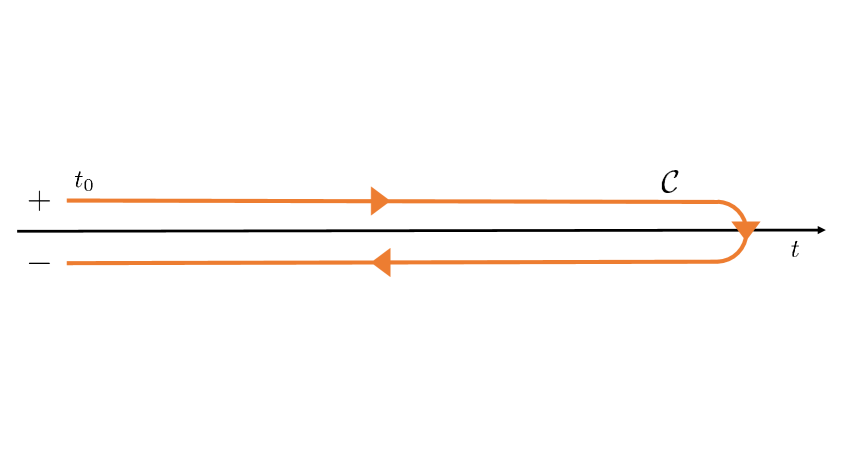
Figure 2: The CTP contour $\mathcal{C}$ in the complex plane of the time variable $t$ with the upper $+$ and the lower $-$ branches starting at the initial time $t_{0}$.

The CTP formalism is aimed at computing time-dependent expectation values $\langle\mathcal{O}(t)\rangle_{\rho}$ for observables $\mathcal{O}$ in an arbitrary state $\rho$, which, in our case, will be represented by the bath of particles in the early Universe. The correlators $\langle\mathcal{O}(t)\rangle_{\rho}$ can be obtained from a path integral in which the time integration contour $\mathcal{C}$ has two branches $\mathcal{C}_{+}$ and $\mathcal{C}_{-}$ going from $-\infty$ to $t$, and from $t$ to $-\infty$, respectively, as illustrated in Fig. 2. As a consequence of the existence of these two branches, the time-ordered two-point correlators of fields along $\mathcal{C}$ can be labeled with two indices $a,b\in\{+,-\}$ which denote the branches at which each the fields in the correlator is evaluated. Representing generic fields of arbitrary spin as $\phi$ and their conjugates (Dirac conjugates in the case of fermions) as $\bar{\phi}$, the Green’s functions can be written as follows,

$$iG^{ab}(x,y)=\big{\langle}T_{\mathcal{C}}\,\phi(x^{a})\bar{\phi}(y^{b})\big{\rangle}.$$ (3.1)

We will use $G=\Delta$ for scalars and $G=S$ for fermions.

As for traditional S-matrix calculations, it is useful to express the Green’s functions in momentum space by performing a Fourier transform with respect to the relative coordinate $r\equiv x-y$. However, in an out-of-equilibrium state, translation invariance is not guaranteed, so that the functions $iG^{ab}(x,y)$ do not necessarily only depend on $x-y$, but may also vary under changes of the average coordinate $(x+y)/2$. Hence, a more suited type of transform to work with is the Wigner transform, defined by

$$G^{ab}(k,x)={\int{\rm d}^{4}r}\,e^{ik\cdot r}G^{ab}\left(x+\frac{r}{2},x-\frac{r}{2}\right)\,.$$ (3.2)

Among the four possible combinations of $G^{ab}$, the $G^{++}$ corresponds to the usual time-ordered Feynman propagators, while $G^{--}$ is a propagator with an inverted time-ordering, with fields sitting on the $-$ branch in Fig. 2. With $G^{++}$ and $G^{--}$ one defines the Hermitian propagator as

$$G^{\mathcal{H}}\equiv\frac{1}{2}\left(G^{++}-G^{--}\right),$$ (3.3)

which can be shown to be the Hermitian part of the retarded propagator. The propagators with mixed branch indices

$$iG^{<}\equiv \,iG^{+-}, iG^{>}\equiv \,iG^{-+},$$ (3.4)

are also called “Wightman functions” and they are of particular importance because related to the so-called spectral (anti-Hermitian) propagator

$$G^{\mathcal{A}}\equiv\frac{i}{2}\left(iG^{>}-iG^{<}\right),$$ (3.5)

which is connected to the phase-space density of propagating degrees of freedom in the chosen state $\rho$ and contains information about their number densities and energy shells. For example, in a free theory with a scalar field of mass $m$ one finds (both in the vacuum and in a thermal state)

$$i\Delta_{0}^{\mathcal{A}}(p)=\pi\,\mathrm{sign}(p^{0})\delta(p^{2}-m^{2}),$$ (3.6)

which gives a nonzero contribution only on the mass-shell $p^{2}=m^{2}$ — and hence is related to the density of states in phase space, as anticipated before — while the Wightman functions also involve the particle distribution functions in equilibrium. Writing the bosonic/fermionic equilibrium densities as

$$f_{\mp}(p^{0})=\frac{1}{e^{p^{0}/T}\mp 1},$$ (3.7)

with $-$ corresponding to bosons, and $+$ for fermions, the free scalar Wightman functions in a state of thermal equilibrium at a temperature $T$, read

$$i\Delta_{0}^{\rm{eq},<}(p)= \,2\Delta_{0}^{\mathcal{A}}(p)\,f_{-}(p^{0}), i\Delta_{0}^{\rm{eq},>}(p)= \,2\Delta_{0}^{\mathcal{A}}(p)\,\left(1+f_{-}(p^{0})\right).$$ (3.8)

The subscript “$0$” indicates that the free propagators are nothing but tree-level propagators, of order zero in the loop expansion of the path-integral with time contour $\mathcal{C}$, which can be obtained by inverting the quadratic terms of the classical action along $\mathcal{C}$ with appropriate boundary conditions. Once one goes beyond free fields and beyond thermal equilibrium, the full propagators differ from the results above. For example, particle distribution functions might not follow their equilibrium values, and there might be corrections to the on-shell relations.

In any case, the distribution functions, and hence the number densities, can still be related to the Wightman functions. For the DM scalar field $s$ with a particle distribution function $f_{s}(\vec{p})$ and number density $n_{s}$, one has

$$f_{s}(\vec{p})=\int_{0}^{\infty}\frac{\differential p^{0}}{\pi}\,p^{0}i\Delta_{s}^{<}(p)\Rightarrow n_{s}=\int\frac{d^{3}p}{(2\pi)^{3}}\,f_{s}(\vec{p})=\int\frac{d^{3}p}{(2\pi)^{3}}\int_{0}^{\infty}\frac{\differential p^{0}}{\pi}\,p^{0}i\Delta_{s}^{<}(p)\,.$$ (3.9)

Note that, in the equilibrium case, this follows immediately from Eqs. (3.6) and (3.8). As a consequence of the relation between number densities and Wightman functions, one can obtain the evolution equation for the DM number density from appropriate dynamical equations for the Wightman functions. In the CTP formalism, such dynamical equations can be derived from the Schwinger-Dyson equations for the two-point functions, which in position space can be expressed in a compact manner in terms of the tree-level propagators $iG^{ab}_{0}$ and bosonic/fermion self-energies $\Pi^{ab},\not{\Sigma}^{ab}$, as follows:

$$i\Delta_{0}^{ab^{-1}}(x,y)=i\Delta^{ab^{-1}}(x,y)+i\Pi^{ab}(x,y)\,,$$ (3.10)

$$iS_{0}^{ab^{-1}}(x,y)=iS^{ab^{-1}}(x,y)+i\not{\Sigma}^{ab}(x,y)\,.$$ (3.11)

The self-energies encode interactions between fields and can be formally defined in terms of two-particle irreducible (2PI) Feynman diagrams with two external legs, and with internal legs corresponding to the full propagators $iG^{ab}$. Equivalently, the self-energies can be obtained as functional derivatives with respect to the corresponding propagators of 2PI vacuum diagrams constructed with full propagators. These vacuum diagrams are part of a generating functional known as the 2PI effective action (cf. A.2) [26, 27, 37, 49, 50]. For the dark matter model considered in this paper, the vacuum diagrams of the 2PI effective action and the corresponding self-energies are illustrated in Eq. 3.24 and Fig. 3, respectively. As the self-energies correspond to loop diagrams with full propagators, the Schwinger-Dyson equations (3.10) and (3.11) constitute a very complicated system of infinitely-many coupled integro-differential equations, which can only be solved if an approximation is performed, for example by truncating the loop expansion to a fixed order. Similarly to the case for the propagators, one can introduce Wightman self-energies as

$$\Pi^{<}\equiv \,\Pi^{+-}, \Pi^{>}\equiv \,\Pi^{-+},$$ (3.12)

as well as spectral and Hermitian self-energies as

$$\Pi^{\mathcal{A}}\equiv \,\frac{i}{2}\left(\Pi^{>}-\Pi^{<}\right), \Pi^{\mathcal{H}}\equiv \,\frac{1}{2}\left(\Pi^{++}-\Pi^{--}\right).$$ (3.13)

Analogous relations hold for $\not{\Sigma}^{<},\not{\Sigma}^{>},\not{\Sigma}^{\mathcal{A}},\not{\Sigma}^{\mathcal{H}}$. The interactions in the plasma captured by the self-energies can introduce decays of a given field into plasma constituents, and can also modify the dispersion relation for the propagating degrees of freedom. In this respect, $\Pi^{\mathcal{A}}/\not{\Sigma}^{\mathcal{A}}$ can be related to decay widths or more general interaction rates, while $\Pi^{\mathcal{H}}/\not{\Sigma}^{\mathcal{H}}$ yield a modification in the fields’ dispersion relations (e.g. changes in the effective pole masses). This connection can be made explicit for the case of a state without spatial and temporal homogeneities, as happens in thermal equilibrium. In this case, the Schwinger-Dyson equations (3.11) for the full propagators can be solved algebraically, leading to so-called “resummed propagators”. For a scalar field, the result is

$${\Delta}^{\rm hom,\mathcal{A}}= \,\dfrac{{\Pi}^{\mathcal{A}}}{\left(k^{2}-m^{2}-{\Pi}^{\mathcal{H}}\right)^{2}+\left({\Pi}^{\mathcal{A}}\right)^{2}}\,,$$ (3.14)

where in the denominator one can recognize a structure leading to a Lorentzian resonance in which the mass in the dispersion relation is shifted by $\Pi^{\mathcal{H}}$, while $\Pi^{\mathcal{A}}$ enters as a width for the resonance. Similarly, in the fermionic case one has

$$\not{S}^{\rm{hom},\mathcal{A}}= \,\left(\not{k}+m-\not{\Sigma}^{\mathcal{H}}\right)\dfrac{\Gamma}{\Omega^{2}+\Gamma^{2}}-\not{\Sigma}^{\mathcal{A}}\dfrac{\Omega}{\Omega^{2}+\Gamma^{2}}\,,$$ (3.15)

with $\not{S}=\gamma^{\mu}S_{\mu}$, $\not{\Sigma}=\gamma^{\mu}\Sigma_{\mu}$ and

$$\begin{aligned} &\Gamma=2\left(k-\Sigma^{\mathcal{H}}\right)\cdot\Sigma^{\mathcal{A}},\\ &\Omega=\left(k-\Sigma^{\mathcal{H}}\right)^{2}-\big{(}{\Sigma^{\mathcal{A}}}\big{)}^{2}-m^{2}\,.\end{aligned}$$ (3.16)

Again, one still has a Lorentzian pole structure, with a width proportional to $\Sigma^{\mathcal{A}}$, and with $\Sigma^{\mathcal{H}}$ modifying the dispersion relation. In the ensuing calculations, we will use resummed propagators for the fermions $F$ and $f$ in thermal equilibrium.

To finalize, we shall mention that in the case of thermal equilibrium, the propagators and self-energies satisfy additional constraints, known as the Kubo-Martin-Schwinger (KMS) relations. For propagators in Wigner space, these are

$$i{\Delta}^{\mathrm{eq},>}(k)= \,e^{\beta k^{0}}i{\Delta}^{\mathrm{eq},<}(k)\,, i\not{S}^{\mathrm{eq},>}(k)= \,-e^{\beta k^{0}}i{\not{S}^{\mathrm{eq},<}}(k).$$ (3.17)

With the anti-hermitian propagators defined as in Eq. (3.5), the previous relations give

$$\begin{aligned} i\Delta^{\mathrm{eq},<}(k)=&\,2\Delta^{\mathrm{eq},\mathcal{A}}(k)f_{-}(k_{0})\,,&i\not{S}^{\mathrm{eq},<}(k)=&\,-2\not{S}^{\mathrm{eq},\mathcal{A}}(k)f_{+}(k_{0})\,,\\ i\Delta^{\mathrm{eq},>}(k)=&\,2\Delta^{\mathrm{eq},\mathcal{A}}(k)(1+f_{-}(k_{0}))\,,&i\not{S}^{\mathrm{eq},>}(q)=&\,2\not{S}^{\mathrm{eq},\mathcal{A}}_{F}(q)(1-f_{+}(q_{0}))\,.\end{aligned}$$ (3.18)

Analogous properties hold for self-energies in equilibrium. In particular, for the DM self-energy arising from the equilibrated fields, one arrives at

$$i{\Pi}^{<}_{s}(p)= \,2f_{-}(p_{0}){\Pi}^{\mathcal{A}}_{s}(p), i{\Pi}^{>}_{s}(p)= \,2(1+f_{-}(p_{0})){\Pi}^{\mathcal{A}}_{s}(p)$$ (3.19)

3.2 Fluid equation for Freeze-in

As summarized in the previous section, the Wightman functions in the CTP formalism contain information about particle number densities, c.f. (3.9). Hence, the Schwinger-Dyson equations for the DM two-point functions $\Delta_{s}^{<}$ associated with the DM scalar field $s$ in our model (cf. Sec. 2) can be turned into an equation for the rate of DM production. While a detailed derivation building on the CTP formalism — outlined with more details in Appendix A — is left to Appendix B, here we give a summary of the strategy and provide the final equation for the DM production rate. The starting point are the Schwinger-Dyson equations (3.10) for $i\Delta_{s}^{<}$ translated into Wigner space, and separated into real and imaginary parts. Assuming spatial homogeneity, one can ignore spatial gradients. Furthermore, as the scalar self-energies $\Pi^{ab}$ are dominated by the contributions of the fields in thermal equilibrium, they are time-translation invariant, so that one can neglect their time derivatives. Taking this into account, the imaginary part of the Schwinger-Dyson equation for $i\Delta_{s}^{<}(k,x)$ in Minkowski space becomes

$$k^{0}\partial_{t}\left(i\Delta_{s}^{<,>}\right) \approx-\frac{1}{2}\left(i{\Pi_{s}}^{>}\,i\Delta_{s}^{<}-i{\Pi_{s}}^{<}\,i\Delta_{s}^{>}\right).$$ (3.20)

To turn this into an equation for the DM production rate, following Eq. (3.9), one can integrate over positive $p^{0}$, leading to

$$\partial_{t}f_{s}(t,\lvert\vec{p}\rvert) =\int_{0}^{\infty}\frac{\differential p^{0}}{\pi}\,\frac{1}{2}\left[\left(i{\Pi}_{s}^{<}\right)\left(i{\Delta}_{s}^{>}\right)-\left(i{\Pi}_{s}^{>}\right)\left(i{\Delta}_{s}^{<}\right)\right].$$ (3.21)

To take things further, one can use the KMS relations (3.18) and (3.19) for the equilibrated fermions and for the DM self-energy. Additionally, we assume that the DM spectral propagator has the form of a tree-level propagator as in Eq. (3.6), as expected for weakly coupled scalar field. Integrating over spatial momenta and accounting for the expansion of the Universe as in Section 2, the final result can be written as

In the equation above, $\Pi^{\mathcal{A}}_{s}(\omega_{p},|\vec{p}|)=\Pi^{\mathcal{A}}_{s}(p^{0},|\vec{p}|)$ is the spectral self-energy of the DM field $s$ in Wigner space, evaluated on the DM momentum shell with $p^{0}$ substituted by the on-shell energy

$$\omega_{p}=\sqrt{|\vec{p}|^{2}+m^{2}_{s}}.$$ (3.23)

The self-energy is dominated by the effects of fields assumed to be in thermal equilibrium — the mediator $F$, the SM fermion $f$, and gauge fields — and as a consequence it is translation invariant, so that one can omit the dependence on the average coordinate in the Wigner transform. Finally, $f_{-}(\omega_{p})$ is a bosonic equilibrium abundance, c.f. Eq. (3.7). A detailed derivation of Eq. (3.22) building on the CTP formalism — outlined with more details in Appendix A — is left to Appendix B. Eq. (3.22) corresponds to the DM rate equation we aim at studying, where the change in time of the DM number density on the l.h.s is controlled by the interaction rate $\gamma_{\mathrm{DM}}$ on the r.h.s. Here, we can see that interactions are determined by the DM spectral self-energy, which is not surprising given the aforementioned connection of $\Pi^{\mathcal{A}}_{s}$ with a width or an interaction rate. Additionally, it turns out that $\Pi^{\mathcal{A}}_{s}$ can be related to the imaginary part of a retarded self-energy, so that Eq. (3.22) can be seen as analogous to the optical theorem for the S-matrix, which relates transition rates to the imaginary part of appropriate amplitudes. We dedicate the following section to the computation and analysis of this fundamental object.

3.3 Production rate and DM self-energy

In this section, we specify the form of the collision term (the interaction rate density) in the DM rate equation (cf. Eq. 3.22). The required DM self-energy can be calculated employing approximations at two levels:

1. the loop order at which the effective action (or, equivalently, the expansion of the DM self-energy) is truncated.

2. The type of propagators appearing in the DM self-energy.

To address the first point, we need the 2PI effective action for our model, which is diagrammatically given by

$$\centering\Gamma_{2}=-i\vbox{\hbox{\includegraphics[height=77.49976pt]{Figures/2PIEA_2loop.pdf}}}\;-i\,\,\vbox{\hbox{\includegraphics[height=73.19421pt]{Figures/2PIEA_3loop.pdf}}}\;+\dots\@add@centering$$ (3.24)

where we used double lines to represent full propagators. The DM scalar lines are dashed, the $F$ and $f$ fermion propagators are solid with a gray and white filling, respectively, while the wavy lines represent gauge bosons. The $\dots$ indicate contributions proportional to further powers of $y_{\text{DM}}$, or higher loops. The self-energies are obtained by taking functional derivatives of $\Gamma_{2}$, corresponding to cutting the diagrams in Eq. (3.24). For instance, let us consider the leading order (LO) contribution at 1-loop to the DM-self-energy, corresponding to 2-loop contributions in the effective action, namely the first term in Eq. (3.24). The resulting DM self-energy is obtained by cutting the DM dashed propagator line in Eq. (3.24) and taking the resulting diagram with external lines amputated, resulting in Fig. 3. Here we also account for both orientations of the fermion loop, corresponding to particle and antiparticle contributions to DM production.

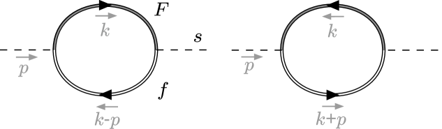
Figure 3: The DM self energy diagrams corresponding to Eq. 3.25. The double lines in the fermion loop indicate a full propagator and we account for contributions coming for both fermion flow orientations.

On the CTP contour, the 1-loop DM self-energy can be written as

$$-i{\Pi}^{ab}_{s}(p)=y_{\text{DM}}^{2}\int\dfrac{\differential^{4}{k}}{(2\pi)^{4}}\tr{P_{L}\,i\,\not{S}^{ab}_{F}(k)\,P_{R}\,i\,\not{S}^{ba}_{f}(k-p)+P_{L}\,i\,\not{S}^{ba}_{F}(k)\,P_{R}\,i\,\not{S}^{ab}_{f}(k+p)}\,,$$ (3.25)

where $ab$ are the CTP indices, $y_{\text{DM}}$ is the DM coupling, $k$ the loop momentum, and where the trace is performed over the Clifford algebra. Using (3.19) together with Eq. (3.25), one can write the spectral self-energy as Substituting the KMS relations for the fermionic propagators in Eq. (3.18) leads to On the CTP, the fermionic self-energy (cf. Fig. LABEL:fig:fermionSelfEn) reads as

$$-i\not{\Sigma}^{ab}(k)_{L/R}=-G_{L/R}\int\dfrac{\differential^{4}{\ell}}{(2\pi)^{4}}\gamma^{\mu}P_{L/R}i\not{S}_{L/R}^{ab}(k-\ell)P_{L/R}\gamma^{\nu}i\Delta^{ab}_{\mu\nu}(\ell)\,.$$ (3.35)

Here, $a,b$ are CTP indices, indicating on which branch of the contour the propagators are evaluated, $P_{L/R}$ are chiral projectors, and the factor $G_{L/R}$ summarizes the gauge interactions of the chiral fermion considered. In the SM case, it is given by Eq. (2.2). Furthermore, $\Delta^{ab}_{\mu\nu}(\ell)$ is the gauge boson propagator which in Feynman gauge is obtained from the scalar propagator by $\Delta^{ab}_{\mu\nu}(\ell)=-g_{\mu\nu}\Delta^{ab}(\ell)$.

The Hermitian and anti-Hermitian self-energies follow from

$$\not{\Sigma}^{\mathcal{H}}\left(k\right)=\frac{1}{2}\left[\not{\Sigma}^{++}\left(k\right)-\not{\Sigma}^{--}\left(k\right)\right]\,,\quad\not{\Sigma}^{\mathcal{A}}\left(k\right)=\frac{1}{2}\left[\not{\Sigma}^{-+}\left(k\right)-\not{\Sigma}^{+-}\left(k\right)\right]\,.$$ (3.36)

In order to compute the quantities in Eqs. (LABEL:eq:OmegaF)-(LABEL:eq:Gammaf) we need to determine the Lorentz-vector $\Sigma^{\mu}_{L/R}$ (where we have suppressed its CTP-indices). This is defined via $\not{\Sigma}_{L/R}=P_{R/L}\gamma_{\mu}\Sigma^{\mu}_{L/R}$ and can be expressed in terms of the Lorentz vectors it depends on, namely $p^{\mu}$, the momentum of the particle, and $u^{\mu}$, the plasma reference vector with $u^{2}=1$ and $u^{0}>0$. In what follows, we choose to work in the rest frame of the plasma, implying $u^{\mu}=(1,\vec{0})$. One can show that the self-energy can be decomposed as

$$\Sigma^{\mu}(k)=\frac{1}{|\vec{k}|^{2}}[(k^{0}u^{\mu}-k^{\mu})\mathcal{K}+(k^{0}k^{\mu}-k^{2}u^{\mu})\mathcal{U}]\,,$$ (3.37)

$$\mathcal{K}\equiv\left(k\cdot\Sigma\right),\qquad\mathcal{U}\equiv\left(u\cdot\Sigma\right)\,,$$ (3.38)

as can be shown by contracting the same expression once with $k^{\mu}$ and once with $u^{\mu}$. These quantities have to be determined for both the Hermitian and anti-Hermitian self-energies. Moreover, they can be decomposed into a vacuum ($T=0$) and a thermal part ($T\neq 0$). The first is given by the full self-energy evaluated in the $T\rightarrow 0$ limit of all distribution functions involved in the calculation, while the latter contains the rest.

The vacuum part of the Hermitian self-energy involves both ultraviolet and infrared divergences. The first need to be renormalized likewise in quantum field theory at zero temperature. The resulting observables (e.g., spectral densities) expressed in terms of renormalized quantities conserve the same analytical form. Importantly, finite-$T$ corrections do not affect the renormalization conditions and do not contain additional UV divergences since there is a natural cutoff at short distances given by the correlation length of thermal fluctuations. We are not interested in the details of the renormalization procedure and, thus, we will assume that our observables have been renormalized in some appropriate scheme. Regarding IR divergences, the Bloch-Nordsiek [115] and the Kinoshita-Lee-Nauenberg [116, 117] theorems make sure that, at zero-temperature, every observable is free of any soft and collinear divergences. The thermal part of the Hermitian self-energy, however, as well as the vacuum and thermal part of the anti-Hermitian self-energy is free of divergences.

The complete derivation of $\mathcal{K}^{\mathcal{H}/\mathcal{A}}$ and $\mathcal{U}^{\mathcal{H}/\mathcal{A}}$ is long and tedious, and parts of them need to be determined numerically. Importantly, we keep the mass of the vectorlike fermion $F$, which complicates the analytical structure, while the SM fermion $f$ can be regarded as massless since we restrict ourselves to DM production in the unbroken electroweak symmetry phase. We leave their full expressions to Appendix C.

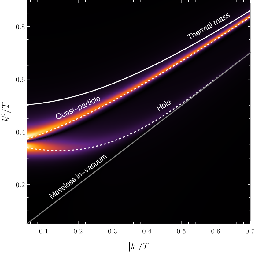
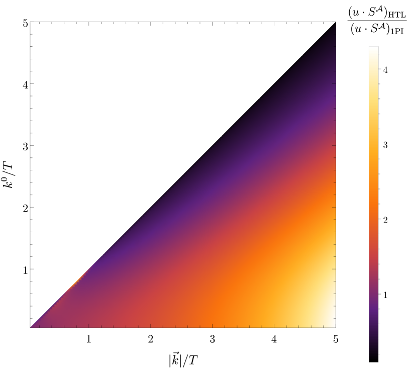
Figure 5: Left panel: the spectral density $(u\cdot S^{\mathcal{A}})_{\mathrm{1PI}}$ in linear scale for a massless fermion as a function of the energy $k^{0}/T$ and spatial $|\vec{k}|/T$ components of its momentum, normalized to the plasma temperature. Brighter colors signal larger values and they are in correspondence of the quasi-particle and hole peaks. Notice how the latter fades away at large momenta as holes decouple from the plasma. The white dashed lines mark the quasi-particle and hole branches in the HTL approximation (cf. Eqs. (3.44) and (3.45)), while the white solid line correspond to the dispersion relation with momentum-independent thermal mass in Eq. (3.46). Notice also that, in the dark regions, $(u\cdot S^{\mathcal{A}})_{\mathrm{1PI}}$ is small but not zero. Right panel: ratio of $u\cdot S^{\mathcal{A}}$ in the HTL approximation to the 1PI one for a broader kinematic range. Below the light cone, the HTL spectral density becomes larger than the 1PI one for hard momenta, which instead captures an exponential suppression as soon as $k\gtrsim T$.

The pole structure of Eqs. (LABEL:eq:SFresummed) and (LABEL:eq:Sfresummed) can be very convoluted and, unless a high-temperature (HTL) expansion is performed (cf. Sec. 3.4.2), its precise form needs some numerical input (cf. Appendix C). In particular, at finite-$T$ there could be several poles representing propagating modes and collective excitations with well-defined quantum numbers [20]. For fermions in a hot plasma, these are usually referred to as screened quasi-particle if they have a positive helicity over chirality ratio, or hole modes if such ratio is negative. These modes can be clearly distinguished in the low-momentum kinematic region, where, as shown in the left panel of Fig. 5, the brighter contours illustrate where the spectral density sharply peaks in correspondence of the poles. In this region, each of the two modes approximately accounts for half the density of states. At large momenta, instead, hole excitations become massless and decouple from the plasma, while the screened quasi-particle modes asymptotically reach the in-vacuum fermionic state. Outside the “mass-shell”, there are also non-zero contributions which can be referred to as “virtual” or “off-shell” modes, where there is energy transfer between the fermion quanta and the thermal bath even if they would be strictly forbidden in vacuum. The contribution in this kinematic regime is proportional to the thermal width $\Gamma$ and, although suppressed, it accounts for the irreducible Landau damping by the medium. Compared to its HTL-approximated version (cf. Sec. 3.4.2), the spectral densities below the lightcone are more damped, as can be seen in the right panel of Fig. 5 .

The DM interaction rate in Eq. (LABEL:eq:RateDensityResummed) receives contributions from four distinct combinations of the spectral densities, depending on whether the fermion momenta ($k$ for the BSM field $F$ and $q$ for the SM field $f$) are above or below their light cone.
$\mathbf{k^{2}>0},$ $\mathbf{q^{2}>0:}$ both fermions have timelike momenta and their spectral densities are peaked at the poles, where a particle-like interpretation of the interacting fermionic states can apply (if the thermal width is sufficiently narrow). The hole peaks lead to negligible DM production compared to the quasi-particle ones and at large momenta they completely decouple. As a result, the DM interaction rate in Eq. (LABEL:eq:RateDensityResummed) is dominated by the kinematics that allow the quasi-particle peaks of the spectral distributions to overlap. In a particle-like interpretation, these contributions can be seen as decay processes of the type $F\rightarrow f+s$ with approximated masses given by $M_{i}^{2}=m_{i}^{2}+m_{\text{th},i}^{2}$, being $m_{i}$ the in-vacuum masses and $m_{\text{th},i}=\sqrt{G}\,T/2$ the thermal masses of the fermions . Since at high temperature the dispersion relations of the two fermions are identical (they receive the same gauge thermal corrections), decays are not kinematically-allowed at early “times” $z=m_{F}/T$, or, in other words, the contribution to DM production from 1PI-resummed spectral densities is suppressed. The kinematic window opens whenever the in-vacuum mass $m_{F}$ starts to be relevant, namely as soon as

$$z>\sqrt{G}\frac{m_{\text{DM}}m_{F}}{m_{F}^{2}-m_{\text{DM}}^{2}}\,.$$ (3.39)

$\mathbf{k^{2}>0}$ and $\mathbf{q^{2}<0}$, $\mathbf{k^{2}<0}$ and $\mathbf{q^{2}>0:}$ this regime constitutes the dominant contribution to the DM interaction rate when the kinematics prevent both fields from being simultaneously on the timelike peaks, as estimated above. The spacelike fermion can be interpreted as a mediator of interactions with the thermal plasma, such that these regimes are seen as scattering processes producing DM quanta.
$\mathbf{k^{2}<0,\,q^{2}<0:}$ when both momenta are spacelike, both spectral-densities are in the continuum and none of them is enhanced from being nearly “on-shell”. Thus, this regime gives the smallest contribution to the DM-interaction rate. In a particle interpretation, they can be viewed as two exchanges of “of-shell” virtual fermion quanta with the thermal plasma.

3.4.2 Resummed propagators in the HTL approximation

The spectral densities obtained in the previous section can be simplified by assuming that the relevant loop momenta $\ell$ in the fermion self-energies are much larger than any other mass scale involved ($k,m_{F},m_{\text{DM}}$) and operating as if a net separation between hard scales $\mathcal{O}(\pi T)$ and soft scales $\mathcal{O}(gT)$ applies. This is, in essence, what goes under the name of Hard Thermal Loop (HTL) effective perturbation theory, where the self-energies resum the leading contributions from thermal fluctuations with hard virtual momenta [43, 42, 110, 111, 112, 113, 114]. In a small coupling expansion, such resummation is necessary any time the external momentum is soft, because, as an explicit calculation would show, contributions that in-vacuum would appear to be of higher order in $g$, in hot theories are effectively of the same order as the tree-level term, breaking the perturbative series in $g$ and requiring its resummation. Practically speaking, we can obtain the HTL-approximated self-energies by operating an expansion in $k/\ell\sim g/\pi$ and considering only the leading terms. Thus, we expect the expansion to be reliable if $g\ll 1$.

We should now ask ourselves if such a scheme, much simpler to work with and often employed in the leptogenesis and DM scenarios, is a reliable one for freeze-in production of DM. The fact that the relevant freeze-in dynamics take place at temperatures $T\sim m_{F}$ would imply that the momentum of the heavy fermion $F$ in the DM self-energy is at least of order $k\sim m_{F}\sim T$, and the expansion parameter $k/\ell$ is a number of order one so that, when calculating the self-energy of $F$, the HTL approximation is not well-justified around the bulk of DM production.

To understand what are the differences with respect to the 1PI-resummed case, in the following we summarize the structure of the HTL self-energy, spectral densities, and production rates. The impact on freeze-in production will be shown in the Result section (cf. Sec. 4). First, we need the HTL limit of the gauge-charged fermion self-energies. The HTL version of $\mathcal{K}_{\mathrm{HTL}}=(k\cdot\Sigma_{\mathrm{HTL}})$ and $\mathcal{U}_{\mathrm{HTL}}=(u\cdot\Sigma_{\mathrm{HTL}})$ reads as

$$\mathcal{K}_{\text{HTL}}^{\mathcal{H}} =\frac{1}{4}G^{2}T^{2}, \mathcal{U}_{\text{HTL}}^{\mathcal{H}}=\frac{G}{8\lvert\vec{k}\rvert}T^{2}\log\left|\frac{k^{0}+\lvert\vec{k}\rvert}{k^{0}-\lvert\vec{k}\rvert}\right|,$$ (3.40)

$$\mathcal{K}_{\text{HTL}}^{\mathcal{A}} =0, \mathcal{U}_{\text{HTL}}^{\mathcal{A}}=\theta\left(-k^{2}\right)\frac{G}{\pi}{8\lvert\vec{k}\rvert}T^{2}\,.$$ (3.41)

Notice that, the functions in Eqs. (3.40) and (3.41) only depend on $T$ and the external momentum, while any in-vacuum mass scale has been neglected in accordance to the high-temperature expansion. We now insert these expressions into Eq. 3.37 and then into the functions $\Omega_{F/f}$ and $\Gamma_{F/f}$ in Eqs. (LABEL:eq:OmegaF)-(LABEL:eq:Gammaf), leading to the HTL-limit of the spectral densities from Eqs. (LABEL:eq:SFresummed) and (LABEL:eq:Sfresummed).

The thermal widths $\Gamma_{F/f}^{\mathrm{HTL}}$, directly proportional to $\mathcal{U}^{\mathcal{A}}_{\mathrm{HTL}}$, are non-zero only for spacelike momenta $k^{2}<0$. In this kinematic regime, we recover the so-called continuum. Analogously to 1PI-resummed spectral densities, the continuum describes Landau damping, with “off-shell” states exchanged with the plasma (notice that a particle picture cannot be established without a properly-defined dispersion relation). However, the HTL continuum parts are less suppressed at large momenta because they do not capture an exponential suppression as soon as $k\gtrsim T$ as we quantify for the $u\cdot S^{\mathcal{A}}$ component in the right panel of Fig. 5. We refer to Appendix D for more details about the analytical structure of the HTL continuum.

For timelike momenta $k^{2}>0$, the HTL widths are vanishing, $\Gamma_{F/f}^{\mathrm{HTL}}=0$, and the HTL spectral densities simplify to delta functions

$$\not{S}^{\mathcal{A}}_{F/f}(k) =\pi\,\text{sign}\big{(}{k^{0}}\big{)}\left(\not{k}-\not{\Sigma}^{\mathcal{H},\mathrm{HTL}}_{F/f}(k)\right)\delta\left(\left[k-\Sigma^{\mathcal{H},\mathrm{HTL}}_{F/f}(k)\right]^{2}-m_{F/f}^{2}\right)\,.$$ (3.42)

where $m_{F/f}$ is the in-vacuum mass, directly appearing from the denominator of the propagator. Here, we recover a situation similar to tree-level in-vacuum spectral densities, with a particle-like behavior featuring a well-defined dispersion relation given by

$$\left[k-\Sigma^{\mathcal{H},\mathrm{HTL}}_{F/f}(k)\right]^{2}-m_{F/f}^{2}=0\,.$$ (3.43)

For a vanishing in-vacuum mass, this equation can be analytically solved by (see, for instance, [123])

$$\left(k^{0}\right)^{2}=\omega_{+}^{2}(\lvert\vec{k}\rvert)=\lvert\vec{k}\rvert^{2}\left[\dfrac{W_{-1}\left(-\exp(-\alpha\lvert\vec{k}\rvert^{2}-1)\right)-1}{W_{-1}\left(-\exp(-\alpha\lvert\vec{k}\rvert^{2}-1)\right)+1}\right]^{2}\,,$$ (3.44)

$$\left(k^{0}\right)^{2}=\omega_{-}^{2}(\lvert\vec{k}\rvert)=\lvert\vec{k}\rvert^{2}\left[\dfrac{W_{0}\left(-\exp(-\alpha\lvert\vec{k}\rvert^{2}-1)\right)-1}{W_{0}\left(-\exp(-\alpha\lvert\vec{k}\rvert^{2}-1)\right)+1}\right]^{2}\,,$$ (3.45)

where $\alpha=16/(GT^{2})$ and where $W_{0}$ and $W_{-1}$ are Lambert-W functions. These solutions physically correspond to the same quasi-particle and hole poles where the 1PI-resummed spectral densities peak, as described in the previous section (cf. left panel of Fig. 5). For a fermion with an in-vacuum mass, an analytic form does not exist and Eq. (3.43) has to be solved numerically. However, note that massive fermions also have two pole branches with similar features. Notably, in the large momentum limit, $\lvert\vec{k}\rvert\gg T$, the quasi-particles have a dispersion relation of the form

$$\left(k^{0}\right)^{2}=\lvert\vec{k}\rvert^{2}+\frac{G}{4}T^{2}\equiv\lvert\vec{k}\rvert^{2}+m_{\text{th}}^{2}\,,$$ (3.46)

where $m_{\text{th}}$ is the thermal mass of the field and it corresponds to the momentum-independent part of the thermal Hermitian self-energy. For fermions interacting with gauge bosons in the plasma, it simply reads as

$$m_{\mathrm{th}}^{2}=\frac{G}{4}T^{2}\,.$$ (3.47)

Inserting the HTL-resummed spectral densities into the DM self-energy in Eq. (LABEL:eq:PiA_master), we can identify the same four kinematic regions and DM production processes discussed at the end of Sec. LABEL:sec:1PI, corresponding to whether the fermionic four-momenta $k$ and $q$ are spacelike or timelike. The DM self-energy is then given by the sum of the four regimes

$$\Pi_{s,\text{HTL}}^{\mathcal{A}}(p)=\Pi_{s,\text{TT}}^{\mathcal{A}}(p)+\Pi_{s,\text{TS}}^{\mathcal{A}}(p)+\Pi_{s,\text{ST}}^{\mathcal{A}}(p)+\Pi_{s,\text{SS}}^{\mathcal{A}}(p).$$ (3.48)

The subscripts TT, TS, ST, SS indicate if the momenta $k$ and $q$ are timelike (T) or spacelike (S). The same interpretations that were outlined for 1PI-resummed spectral densities, also apply in the HTL case, with some adjustments. For instance, above the light cone, the vanishing thermal width implies that we do not have anymore resonant peaks, but delta-functions which strongly constraint which momenta give a non-zero DM production rate. If “decay” processes are the dominant one, we should expect 1PI-resummed and HTL spectral densities to yield a similar DM abundance for small gauge couplings (the 1PI-resummed peaks are quite narrow), but be dissimilar as soon as widths become wider and the HTL approximation less reliable at larger $G$ (which is indeed the case, as outlined in Sec. 4). Moreover, as already discussed, HTL spectral densities are not as suppressed as 1PI-resummed ones at spacelike momenta because the in-vacuum mass of the vectorlike fermion $F$ is neglected (cf. right panel of Fig. 5). Therefore, HTL propagators are expected to lead to larger DM production from scattering processes compared to 1PI-resummed ones. As we will show in Sec. 4, such differences will have the largest impact on the DM relic abundance precisely when decay production is kinematically forbidden and scattering processes are the only available channels.

3.4.3 Tree-level propagators

We now take the tree-level limit of the HTL fermionic spectral densities, that is to say we consider only the leading-order correction in $gT$ to the HTL fermionic self energies. This implies that the thermal widths are identically zero and that in the dispersion relations we only retain the momentum-independent thermal masses (cf. Sec. 3.4.3). In this way, the spectral densities in the DM self-energy loop simplify to delta functions defined above the light cone, yielding

$$\not{S}^{\mathcal{A}}_{F}(k)=\pi\delta(k^{2}-m_{F}^{2})\big{(}{\not{k}+m_{F}}\big{)}\,\text{sign}\big{(}{k^{0}}\big{)}\,,$$ (3.49)

$$\not{S}^{\mathcal{A}}_{f}(k-p)=\pi\delta\big{(}{(k-p)^{2}-m_{f}^{2}}\big{)}\big{(}{\not{k}-\not{p}+m_{f}}\big{)}\,\text{sign}\big{(}{k^{0}-p^{0}}\big{)}\,,$$ (3.50)

where the masses are only determined by the in-vacuum masses and the (momentum-independent) thermal masses. In analogy to what we have discussed in the previous sections, such a configuration corresponds to only accounting for DM production from decays of on-shell fermionic states with in-vacuum and thermal masses as in Eq. (3.46). To obtain the tree-level limit of the DM self-energy, we insert these expressions into Eq. (LABEL:eq:PiA_master), yielding

$$\Pi^{\mathcal{A}}_{s}(p)=4\pi^{2}y_{\text{DM}}^{2}\int\dfrac{\differential^{4}{k}}{(2\pi)^{4}}\delta(k^{2}-m_{F}^{2})\delta\big{(}{(k-p)^{2}-m_{f}^{2}}\big{)}\big{(}{k^{2}-k\cdot p}\big{)}$$

$$\hskip 113.81102pt\times\left[1-f_{+}(k_{0})-f_{+}(p_{0}-k_{0})\right]\,\text{sign}\big{(}{k_{0}}\big{)}\text{sign}\big{(}{k_{0}-p_{0}}\big{)}\,.$$ (3.51)

This integral can be analytically resolved. For instance, by transforming the integration measure with

$$\differential^{4}k\longrightarrow\frac{1}{2\lvert\vec{p}\rvert}\differential\phi\,\differential k_{0}\,\differential(p\cdot k)\,\differential(k^{2})\,,$$ (3.52)

it is easier to perform the integration over the delta functions. Moreover, since the particles in the loop are forced to be on-shell, one can show that

$$\text{sign}\big{(}{k_{0}}\big{)}\,\text{sign}\big{(}{k_{0}-p_{0}}\big{)}=-\text{sign}\big{(}{p^{2}-m_{F}^{2}-m_{f}^{2}}\big{)}\,.$$ (3.53)

With these observations at hand, we can turn Eq. (3.4.3) into

$$\Pi^{\mathcal{A}}_{s}(p)=\dfrac{y_{\text{DM}}^{2}}{16\pi\,|\vec{p}|}\Big{|}p^{2}-m_{F}^{2}-m_{f}^{2}\Big{|}\int_{\mathcal{B}}\differential k_{0}\,\Big{[}1-f_{+}(k_{0})-f_{+}(p_{0}-k_{0})\Big{]}\,,$$ (3.54)

where the integration boundaries of the integral $\mathcal{I}$ are such that

$$\mathcal{I}\Big{|}_{\mathcal{B}}=\mathcal{I}\Big{|}_{k_{-}^{0}}^{k_{+}^{0}}\,\theta\big{(}{p^{2}}\big{)}+\mathcal{I}\Big{|}_{-\infty}^{+\infty}\,\theta\big{(}{-p^{2}}\big{)}\,,$$ (3.55)

with

$$k_{\pm}^{0}=\frac{p_{0}}{2p^{2}}\left(p^{2}+m_{F}^{2}-m_{f}^{2}\right)\pm\frac{\lvert\vec{p}\rvert}{2p^{2}}\sqrt{\lambda\left(p^{2},m_{F}^{2},m_{f}^{2}\right)},$$ (3.56)

$$\lambda\left(p^{2},m_{F}^{2},m_{f}^{2}\right)=\left(p^{2}-(m_{F}+m_{f})^{2}\right)\left(p^{2}-(m_{F}-m_{f})^{2}\right)\,.$$ (3.57)

By integrating the expression in Eq. (3.54), accounting for the full distribution functions at finite-temperature, we obtain

$$\Pi^{\mathcal{A}}_{s}(p)=\dfrac{y_{\text{DM}}^{2}}{16\pi\lvert\vec{p}\rvert}\Big{|}p^{2}-m_{F}^{2}-m_{f}^{2}\Big{|}\left(p_{0}\,\theta(-p^{2})+T\ln\left|\dfrac{\cosh\big{(}{(p_{0}-k^{0}_{-})/2T}\big{)}}{\cosh\big{(}{(p_{0}-k^{0}_{+})/2T}\big{)}}\,\dfrac{\cosh\big{(}{k^{0}_{+}/2T}\big{)}}{\cosh\big{(}{k^{0}_{-}/2T}\big{)}}\right|\right)\,.$$ (3.58)

Finally, the differential interaction rate with $p^{2}=m_{\text{DM}}^{2}>0$ and $p_{0}=\omega_{p}=\sqrt{m_{\text{DM}}^{2}+\lvert\vec{p}\rvert^{2}}$ reads as

$$\dfrac{\Pi^{\mathcal{A}}_{s}(p)}{\omega_{p}}=\dfrac{y_{\text{DM}}^{2}\,T}{16\pi\,\omega_{p}\,\lvert\vec{p}\rvert}\Big{|}m_{\text{DM}}^{2}-m_{F}^{2}-m_{f}^{2}\Big{|}\,\ln\left|\dfrac{\cosh\big{(}{(\omega_{p}-k^{0}_{-})/2T}\big{)}}{\cosh\big{(}{(\omega_{p}-k^{0}_{+})/2T}\big{)}}\,\dfrac{\cosh\big{(}{k^{0}_{+}/2T}\big{)}}{\cosh\big{(}{k^{0}_{-}/2T}\big{)}}\right|\,.$$ (3.59)

Notice that, the differential rate can in principle describe both decays and inverse decays, depending on the kinematic regions. In our setup, the hierarchy is well-established as $m_{F}>m_{f}+m_{\text{DM}}$ holds at any temperature, and kinematics would select only $F~{}\rightarrow~{}f~{}+~{}s$ decays. Since we used Fermi-Dirac distribution functions, their inclusion translate into the appearance of the hyperbolic cosines. For Bose-Einstein statistics one would find hyperbolic sine functions. The same differential rate can be derived from a Boltzmann equation approach by only accounting for decays without approximating the equilibrium distribution functions to Maxwell-Boltzmann ones [10, 11, 13]. Notice that, the CTP formalism allows us to directly account for the quantum relativistic nature of the interacting particles from a first principle approach.

The total DM production rate $\gamma_{\mathrm{DM}}$ from decays (with relativistic quantum statistics accounted for) can be obtained simply by integrating Eq. 3.59 over $\differential\lvert\vec{p}\rvert$. Similar to the HTL situation, when compared to 1PI-resummed spectral densities, we shall expect such an approximation to yield the largest discrepancy at the level of the DM relic abundance whenever decay processes are suppressed (small mass splitting between $F$ and DM), and when a high-temperature and small-coupling expansion is not reliable anymore. In addition to the HTL case, however, tree-level propagators completely miss scattering contributions, so that we should expect much less DM then with 1PI-resummed spectral densities when these processes are expected to be relevant (especially for small mass splittings and large gauge couplings), as we will see in the next section.

4 Comparing the 1PI-resummed calculation with other approaches

In this section, we discuss the interaction rate densities $\gamma_{\text{DM}}$, and the relic abundance of DM, defined by Eq. (2.9), obtained in the various approaches previously described in this article. In particular, we want to compare the results obtained based on the 1PI-resummed propagators in the CTP formalism (cf. Sec. LABEL:sec:1PI) with the other, in the literature well established approaches:

• the Boltzmann approach including decays with in-vacuum mass, where the DM interaction rate density is given in Eq. (2.10).

• the Boltzmann approach including decays with in-vacuum and thermal masses, where the DM interaction rate density is given in Eq. (2.11).

• the Boltzmann approach including both decays with in-vacuum and thermal masses, and scatterings with propagators regulated by thermal masses, where the interaction rate density is given in Eq. (2.14).

• the CTP approach with tree-level propagators, where the DM interaction rate density is given in Eq. (3.22) evaluated with Eq. (3.59).

• the CTP approach with HTL-approximated 1PI-resummed propagators, where the DM interaction rate density is given in Eq. (3.22) evaluated with Eq. (3.48).

Notice that, as previously discussed, for the methods relying on the CTP, we take into account the full relativistic quantum statistics, while in the three scenarios using the Boltzmann equation we employ non-relativistic Maxwell-Boltzmann distribution functions.

4.1 Interaction rate densities

We start by comparing the interaction rate densities derived in the previous section. This allows us to identify where and how the various approximations deviate from the 1PI-resummed result using the CTP formalism – the central result of this work.

4.1.1 Numerical procedure

We first normalize each dimensionful parameter to the plasma temperature such that we can operate with dimensionless variables. Then, we fix the free parameters

$$G,\quad\delta=\frac{m_{F}-m_{\text{DM}}}{m_{F}},\quad z\equiv m_{F}/T,$$ (4.1)

where $\delta$ is the relative mass splitting between the mediator and DM, while $G$ is the effective gauge coupling defined in Eq. (2.2). In particular, we scan over $G\in\left[0.4,1.6\right]$ in steps of $0.1$ and $\log_{10}\delta\in\left[-1,1\right]$ in steps of $2/9$, for $32$ values of $z$ between $z=0.01$ and $z=10$, resulting in $13\times 10\times 32~{}=~{}4160$ parameter points. The interval for $G$ is motivated by some of the typical values the running gauge couplings assume at one-loop order, when considering different gauge quantum number assignments for the parent particle at several energy scales $\mu$ (cf. Tab. 1). This energy scale is identified with the energy scale where DM production dominantly takes place, which is well described by the maximum of the parent particle mass $m_{F}$ and the temperature $T$, such that the effective gauge couplings runs when $z<1$. We estimated the changes on the relic density induced by running effects when $G(\mu=\text{max}\left[m_{F},T\right])$ compared to a constant effective gauge coupling defined via $G(\mu=m_{F})$ by assuming a color-dominated effective gauge coupling. We employ $\beta$-functions at one-loop and we only consider contributions from scatterings (which dominate for $z<1$) for this estimate. We find that corrections are at most $\mathcal{O}(1\%)$, as expected from the logarithmic dependence of the running on $z$. Thus, in the following, we assume a constant effective gauge coupling, evaluated at the energy scale of the vacuum mass $m_{F}$ of the heavy vectorlike fermion.

Since what we have discussed so far only applies in the unbroken phase of the electroweak (EW) symmetry, our computation is reliable if freeze-in happens before its breaking, namely if $T_{\text{fi}}\simeq m_{F}/5\gtrsim T_{\text{EW}}$, where $T_{\text{EW}}\simeq 160\,\text{GeV}$ [124]. Thus, for masses above $m_{F}\gtrsim\text{TeV}$, we can safely assume that DM production lies in the EW unbroken phase.

Figure 6: Evolution of the interaction rate density in terms of the time variable $z=m_{F}/T$ for a calculation using: the Boltzmann equation (BEQ) including decays only (blue and short dashing), scatterings (blue and long dashing) with thermal masses and their sum (solid blue). The rate from decays with in-vacuum masses is shown with solid green lines. In the CTP formalism, the rates are derived with 1PI-resummed propagators (red, solid), using HTL propagators (red, long dashing), and tree-level propagators (red, short dashing). The latter also corresponds to decays with thermal masses and full quantum relativistic statistics.

The integration in Eq. (LABEL:eq:RateDensityResummed) is performed numerically for each of the considered $4160$ parameter points, by employing the VEGAS adaptive Monte Carlo integration algorithm [125] of the GNU Scientific Library [126]. We make sure that the results of the integration feature an estimated error of at most $1\%$. In Fig. 4.1.1, we present the time-evolution of the interaction rate densities for the various methods described in the previous sections for four different benchmark parameter choices, $(G,\delta)=\left\{(1.2,1),(1.2,0.1),(0.5,1),(0.5,0.1)\right\}$.

For the case of 1PI-resummed and HTL-resummed propagators, we fit the values of $\gamma_{\text{DM}}$ obtained with the numerical integration by using the following function

$$\frac{\gamma_{\text{DM}}(z)}{y_{\text{DM}}^{2}T^{4}}=Az^{3}K_{1}\left(az\right)+BzK_{1}\left(bz\right)\,,$$ (4.2)

where $A$, $a$, $B$ and $b$ are the parameters of the fit and depend on the parameters $G$ and $\delta$ and where $K_{1}(z)$ is a modified Bessel function of the second kind. We have verified that, the relic density obtained with the fitted function does not deviate more than $2\%$ from the relic density obtained from a linear interpolation of our data points. In Fig. 7, we show the numerically obtained data points using 1PI-resummed propagators as well as the fit using Eq. (4.2) for two exemplary data points.

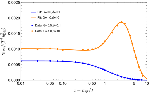
Figure 7: We display the numerically obtained data points for the DM interaction rate density using 1PI-resummed propagators, as well as our fit to the data for two choices of $(G,\delta)$.

The results are shown with solid (long-dashed) red lines in Fig. 4.1.1 for the 1PI-resummed (HTL-resummed) propagators. The form of this function is motivated by the behavior of the interaction rate in the high- and low- temperature regimes: At high-temperatures (small $z$), decays are suppressed and, eventually, kinematically forbidden (cf. Eq. (3.39)), while scatterings dominate due to the enhanced number density of potential scattering partners ($n^{\text{eq}}\sim T^{3}$). The interaction rate for scatterings in vacuum typically behaves as $\sim zK_{1}\left(z\right)$, motivating the second term in Eq. (4.2). Notice that, if $z\ll 1$, this term is approximately constant in $z$, explaining why we see a plateau in Fig. 4.1.1. Since at high temperatures the mass splitting between the parent and the DM candidate becomes negligible, the strength of the scattering contribution is solely regulated by its direct proportionality to the effective gauge coupling $G$, explaining why the plateau at small $z$ is higher for larger $G$. Thus, we expect the fitting parameter combination

$$Az^{3}K_{1}\left(az\right)+BzK_{1}\left(bz\right)\overset{z\rightarrow 0}{\sim}\frac{B}{b}\,,$$ (4.3)

to exclusively depend on $G$. We are able to estimate a functional dependence of the fitting parameters based on the assumption that, at high-$T$, the interaction rate is dominated by scatterings involving one gauge boson vertex ($\propto G$) and featuring fermions exchanged in the $t$-channel ($\propto G\ln G$) [69]. By fitting the data obtained with 1PI-resummed spectral densities, we find

$$\frac{B}{b}=5\cdot 10^{-4}\,G-1.66\cdot 10^{-4}\,G\ln G\,.$$ (4.4)

At low-temperatures ($z\gtrsim 1$), parent particle decays constitute the dominant contribution to the interaction rate density, as long as the mass splitting is large enough to kinematically allow them (cf. Eq. (3.39)) while the parent particles are sufficiently abundant. In this case, the interaction rate typically behaves as $\sim z^{3}K_{1}\left(z\right)$, explaining the first term in Eq. (4.2) and the peaks observed in Fig. 4.1.1 for $\delta=10$. Up to small corrections in $G$, the height of the peak is mainly controlled by the mass splitting $\delta$. Notice that, by lowering $\delta$, the contribution from decays becomes increasingly negligible due to the suppression of the available phase space, until they disappear for degenerate masses. For large $z$ values we can identify the following asymptotic behavior

$$Az^{3}K_{1}\left(az\right)+BzK_{1}\left(bz\right)\overset{z\rightarrow\infty}{\sim}\frac{A}{\sqrt{a}}\,.$$ (4.5)

For decay-dominated freeze-in, one typically has $A/\sqrt{a}=\Gamma_{F}/m_{F}^{2}$, $\Gamma_{F}$ being the decay width in vacuum of the decaying $F$ parent. Since this identification is only valid in the non-relativistic expansion, we can simply use in-vacuum masses to evaluate $\Gamma_{F}/m_{F}^{2}$ and thus obtain a parametric dependence only on the mass splitting of the form

$$\frac{A}{\sqrt{a}}=0.033\frac{\delta^{2}\left(\delta+2\right)^{2}}{16\pi\left(1+\delta\right)^{4}}\,.$$ (4.6)

4.1.2 Interpretation

Let us now compare the solutions obtained using HTL-resummed (long-dashed red lines) and tree-level propagators (short-dashed red lines) to our main result obtained using 1PI-resummed propagators (solid red lines) within the CTP formalism as shown in Fig. 4.1.1.
CTP with HTL resummed propagators: Overall, the HTL-resummed solution has a larger contribution from scatterings, while the rates are similar in the decay-dominated regime (large $z$). In the transition region around $z\sim 1$, the HTL solution underestimates the interaction rate density. These effects can be understood as follows: for small $z$, where scatterings dominate, the leading contribution comes from momentum configurations where one of the two fermionic propagators has a spacelike momentum. Since the HTL approximation neglects the in-vacuum mass of the parent, it fails to capture an exponential suppression at large spacelike momenta, instead present in the 1PI-resummed propagator (cf. Fig. 5), causing the larger rate in this regime. On the other hand, decays start to become relevant as soon as the dispersion relations of the $F$ and $f$ fermions allow for a decay to take place. This is a rather strict statement for HTL-resummed propagators, which, for timelike momenta, are delta functions. On the contrary, 1PI-resummed propagators have finite widths even for timelike momenta such that the “smeared” spectral densities allow to capture the decay contribution for a wider range of momenta, also at smaller $z$ values (explaining why the red solid lines rise earlier in Fig. 4.1.1). This effect is enhanced for large values of $G$. As soon as the decays are fully accessible, HTL rates overestimate the decay contribution for the same reason: the finite width of the 1PI-resummed propagators smear-out the quasi-particle peak, leading to a slight reduction of the rate when the quasi-particle solutions are kinematically accessible.
CTP with tree-level propagators: In this set-up, the rate is computed with Eq. (3.59) and accounts only for decays with thermal masses and quantum relativistic statistics, but omits any scattering contribution. This rate is equivalent to the one obtained with HTL timelike propagators, when approximating $(\Sigma_{F/f}^{\mathcal{H}})^{2}=m_{\text{th}}^{2}$. Therefore, the interpretation follows closely, what we have just discussed above for decays in the HTL approximation.
Boltzmann approach with decays and scatterings using thermal masses: By using thermal masses, we underestimate scattering contributions, whereas the contributions coming from decays is generically larger. The first feature is a consequence of the use of Boltzmann statistics instead of the accurate quantum statistics when calculating the collision term. The overestimate for larger $z$, on the other hand, could originate for multiple reasons. Firstly, accounting for the appropriate Bose-Einstein and Fermi-Dirac distributions (red short-dashed lines) implies that final-state fermions are disfavoured by Pauli blocking, so that simply using Boltzmann statistics (blue short-dashed lines) enlarges the decay contribution. In addition, as indicated in Fig. 5, approximating the fermion dispersion relations only with in-vacuum and thermal masses tend to overestimate the total mass, increasing the decay contribution when decays are efficient. At the same time, a larger thermal mass also leads to an earlier closure of the kinematically-allowed window for decays. Furthermore, we find that thermal mass regulated scatterings have a non-negligible effect significantly longer than what obtained with 1PI-resummed propagators. These differences explain why the height of the decay peaks is not the same for the solid blue and red curves.
Boltzmann approach with vacuum decays: This method does not consider scattering contributions and thus strongly underestimates the production rate at small $z$. For larger $z$, where decays dominate the interaction rate, it lies in between the rates obtained from decays with thermal masses and the CTP rates. The reduced rate compared to the rate including the scattering contribution (solid blue) can be explained mostly from the neglected scatterings as well as the neglected thermal masses.

4.2 Relic density

Figure 8: Evolution of the DM relic abundance. The color scheme of the plotted lines and the values of $G$ and $\delta$ chosen in each panel are the same as in Fig. 4.1.1.

We now compare the different predictions to the DM relic density from the methods discussed in the previous section. In Fig. 4.2, we plot the time-evolution of the relic density in Eq. (2.9) based on the different evaluated interaction rate densities discussed above and depicted in Fig. 4.1.1. The results obtained in the CTP formalism from Eq. (3.22), by employing 1PI-resummed propagators (cf. Sec. LABEL:sec:1PI) are displayed with red solid lines and their HTL-resummed version (cf. Sec. 3.4.2) in red-dashed, while the solution using tree-level propagators with thermal masses is shown in red short-dashed lines. In addition, green solid lines represent the relic density evolution obtained in the Boltzmann equation approach using decays with vacuum masses only, see Eq. (2.10), while the relic density including decays with in-vacuum and thermal masses (Eq. (2.11), dot-dashed blue) and scattering processes (dashed blue) according to Eq. (2.14) result in the solid blue curves. This color scheme is in complete analogy to Fig. 4.1.1. We show the results for the four benchmark points $G=\left\{1.2,0.5\right\}$ and $\delta=\left\{0.1,10\right\}$.

Generally speaking, one finds that for small mass splittings $\delta$ scattering contributions dominate the relic density, while decay contributions constitute the dominant production channel for larger $\delta$.

Figure 9: Evolution of the DM relic abundance normalized to the values obtained with 1PI-resummed propagators. The color scheme of the plotted lines and the values of $G$ and $\delta$ chosen in each panel are the same as in Fig. 4.1.1.

Finally, in the $(G,\delta)$-plane of Figs. 10-14 we show the percentage deviations of the relic density obtained with the methods outlined in this section to the main new result of this article obtained with 1PI-resummed propagators. We also indicate with a color scheme if such methods lead to a larger (yellow to red colors) or smaller (azure to blue colors) DM abundance. We state and briefly discuss the accuracy of each method in the following.

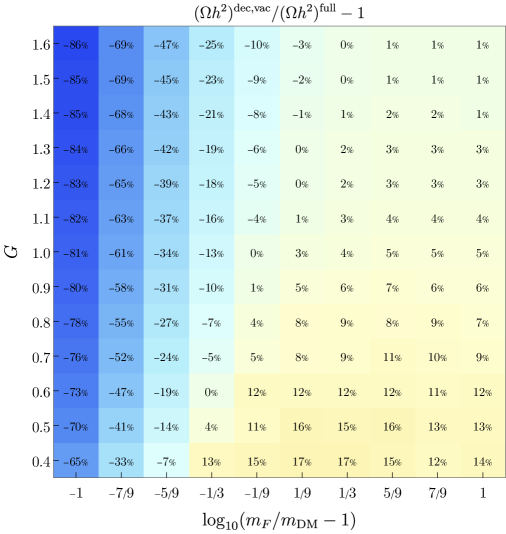
Figure 10: Relative correction on the relic abundance calculated with taking into account one-loop fully-resummed propagators with respect to the one calculated within the Boltzmann approach only considering vacuum decays. The percentage deviation is also shown in warm colors when positive, and with cold colors when negative.

Boltzmann approach with decays (vacuum masses): This approach does not include any DM production from scatterings, while it overestimates DM production from decays. As a consequence, as shown in Fig. 10, the rate tends to moderately overestimate the relic density for large $\delta$ (up to $14\%$), while it strongly underestimates it for small $\delta$ (up to $-86\%$), where decay contributions are suppressed. We notice that there exists a region in parameter space, where the overestimated decay contribution precisely compensates the neglected scatterings, corresponding to a diagonal across the plane in Fig. 10. This explains why the overproduction (underproduction) of DM for large (small) $\delta$ becomes softer (stronger) for higher values of $G$.
Boltzmann approach with decays (thermal masses): as previously elaborated, decays with thermal masses tend to overestimate DM production in the non-relativistic regime, while no DM particle is produced at high temperatures due to kinematic constraints. As a consequence, as shown in Fig. 11, the rate also tends to moderately overestimate the relic density for large $\delta$ (up to $15\%$), while it even more strongly underestimates it for small $\delta$ (up to $-100\%$), where decay contributions are suppressed. This effect is exaggerated when including the relativistic quantum statistics, where Pauli blocking further reduces the production rate, an effect captured by employing tree-level propagators in the CTP formalism (cf. Fig. 12). Thus, remarkably, including only decays with thermal masses yields the largest deviation from the 1PI-resummed result. Overall, neglecting DM production from scatterings leads to the largest deviations for the highest values of $G$ as the scattering contributions are directly proportional to powers of the gauge couplings (cf. Eq. (4.4)). As when considering vacuum decays, there exists a region in parameter space, where the overestimated decay contribution precisely compensates the neglected scatterings, which is evident in Fig. 11.
Boltzmann approach considering decays and scatterings with thermal masses: we improve on the previous calculation by adding scattering contributions with $t$-channel propagators regulated by thermal masses. The results are summarized in Fig. 13. Again, DM is overproduced at large $\delta$ because of the overestimated production rate from decays, resulting in up to $\sim+35\%$ values of $\Omega_{\text{DM}}h^{2}$. Additionally, for $\delta\lesssim 25\%$, deviations of the relic density are found to be negative up to $\sim-10\%$, due to the fact that scatterings, dominating in this parameter region, yield a lower rate compared to the 1PI-resummed calculation. As in the previous scenario, the two effects can cancel each other for moderate mass splittings and gauge couplings, resulting in only $\mathcal{O}(1\%)$ deviations. Furthermore, since the $G$ dependence of the scattering contribution is now taken into account, the relative deviation is only very mildly dependent on $G$ and almost entirely controlled by the mass-splitting. The accuracy of this method can be further enhanced if the correct quantum statistics of the bath particles are considered. While we have not performed this calculation for the scattering contribution, the effect for decays is exactly captured by the solution using tree-level propagators with thermal masses. Such a treatment reduces the deviation for large mass splittings to $\sim+15\%$.
HTL propagators: As explained in the previous section, the HTL-approximated results provide a relatively accurate description of the decay contribution, whereas they tend to overestimate DM production from scatterings, as summarized in Fig. 14. Consequently, using HTL propagators deviates from the results with 1PI-resummed up to only a few percent at large mass-splittings where decays dominate, while they lead to more DM abundance (up to $+27\%$) for smaller $\delta$. Additionally, the deviation increases with $G$, an effect that was to be expected since the HTL expansion is effectively an expansion in $G/\pi$.

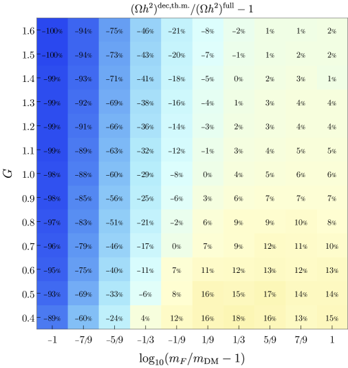
Figure 11: Same caption as Fig. 10 but considering vacuum and thermal masses instead of only vacuum masses.

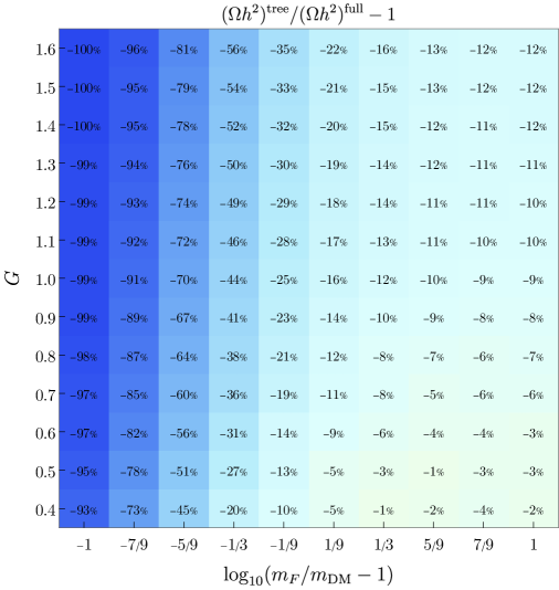
Figure 12: Same caption as Fig. 10 but considering vacuum and thermal masses as well as the correct quantum statistics instead of vacuum masses only and Boltzmann statistics.

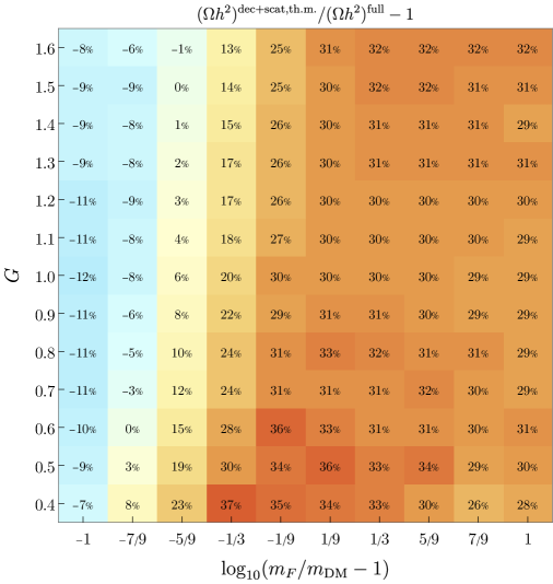
Figure 13: Same caption as in Fig. 10, but including thermal masses for decays as well as thermal mass regulated scatterings.

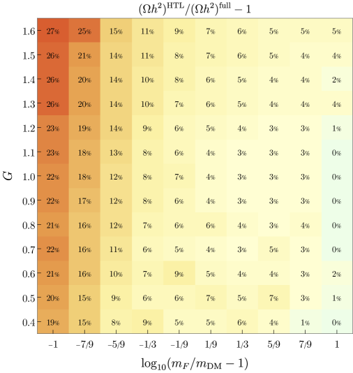
Figure 14: Relative correction on the relic abundance calculated with taking into account one-loop fully-resummed propagators with respect to the one calculated with HTL-resummed propagators in the real-time formalism. The percentage deviation is also shown in warm colors when positive, and with cold colors when negative.

In summary, we have highlighted the complexity of incorporating thermal corrections from the plasma, revealing that various methods yield different results when compared to the ab-initio calculation on the CTP with 1PI-resummed fermion propagators, including the mediator $F$ and DM in-vacuum masses.

The semi-classical Boltzmann approach only considering decays does not provide a universally good description of DM freeze-in production since it can deviate up to $100\%$ ($86\%$) if thermal masses are (not) included. It is noteworthy that including thermal masses when only considering decays decreases the accuracy for this class of models. If however scatterings, where $t$-channel scatterings are regulated by thermal masses, are included, this result improves dramatically at small mass-splittings to deviations of $\mathcal{O}(-10\%)$, but lead to $\mathcal{O}(35\%)$ more DM when the heavy mediator decays dominate its production. In this case, deviations are almost independent of the precise value of $G$.

This picture changes when considering a method that also relies on the CTP formalism. The DM relic abundance from HTL-resummed propagators agrees at the percent level when the mass hierarchy between the two dark sector states is large, but leads to up to $\mathcal{O}(25\%)$ more DM in the mass-compressed region. The largest deviation is found for the highest values of the effective gauge coupling $G$. Using tree-level propagators, on the other hand, completely misses DM production from scatterings in the ultrarelativistic regime, leading to up to $\mathcal{O}(100\%)$ less DM today at small $\delta$, but to a similar amount compared to our main calculation when decays are mostly relevant ($\delta=10$).

We want to stress that our findings are applicable to any model of scalar DM where the DM production vertex involves particles that dominantly interact via gauge-interactions. For models featuring top quarks, the Yukawa-induced corrections to the fermionic self-energies lead to a disproportion between the fermionic dispersion relations, with top quarks being more energetic due to the larger thermal masses. Including these corrections would change the window in time where DM production from decays efficiently contributes to the production rate and therefore would have significant implications for the comparison of the various methods discussed.

We would like to quantify the size of contributions to the relic density omitted in this work. As discussed previously, we truncate the expansion of the 2PI effective action at leading order. This truncation results in the omission of two potentially relevant contributions. Firstly, interference terms of $t$-channel and $s$-channel scatterings only arise at NLO in the expansion of the 2PI effective action and are thus not included. On the level of the Boltzmann equation, however, we find them to be sub-leading (around $\mathcal{O}(10\%)$) compared to squared $s-$ and $t$-channel contributions and expect similar contributions with our method. Secondly, in this way we do not yet include contributions to DM production arising from the LPM effect. In Ref. [39], the authors analyze a similar scenario to ours (with different statistics: a scalar mediator and fermionic DM) and show that the LPM effect amounts to an enhancement of the contribution from scatterings to the DM relic abundance of order $\mathcal{O}(50\%)$ ($10\%$) for small (large) mass splittings. These results, however, are obtained in the ultrarelativstic limit and interpolated to smaller temperatures. The treatment of the LPM effect involving two in-vacuum mass scales, as in our scenario, is not yet discussed in the literature up to today and is part of a follow-up work. This makes a precise estimate of the effect challenging at this point. To give an indication of the corrections that we expect, we estimate the maximal effect on our results in the following way: Based on Ref. [39], we assume that the LPM effect enhances the DM production rate from scatterings by $50\%$ for $\delta=0.1$ and by $10\%$ for $\delta=10$ and linearly interpolate the enhancement in $\delta$ in between. We then compare the resulting DM relic density to the one without this correction. The results of this comparison are presented in the $(G,\delta)$-plane in Fig. 15, where we employ the same figure style as for our previous comparisons. We find that, when truncating the effective action at LO, the relic density can be underestimated by up to $31\%$ for the smallest mass splittings, when scatterings dominate the DM interaction rate. For large mass splittings, the relic density is only mildly affected and differs by few percents.

Related to the previous point is another source of theoretical uncertainty, which is related to the non-conservation of local symmetries. In fact, truncating the loop-expansion of the 2PI effective action, as done in this work, prevents the gauge-dependent parts of diagrams of higher-loop topologies to cancel each other, leading to gauge-dependent observables [127, 128, 129, 130, 72]. In practice, however, a truncation and a gauge choice have to be performed, which in our case correspond to considering the LO (two-loop) expansion of the 2PI effective action and the Feynman gauge. Thus, we expect any omitted gauge-dependent contribution to the 1PI-resummed propagators and to the DM relic abundance to fall within the uncertainty band of the higher-order corrections that were not accounted for in our calculation.

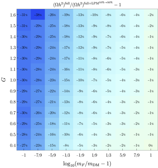
Figure 15: Relative correction to the relic density calculated with 1PI-resummed propagators when further considering a $50\%$ ($10\%$) enhancement of the scattering rate producing DM for $\delta=0.1$ ($\delta=10$), the estimated contribution of the LPM effect from Ref. [39]. For mass splittings in between we linearly interpolated the enhancement in $\delta$. The percentage deviation is shown in colder colors when more negative.

5 Conclusions and Recommendations

In this article, we have analyzed finite-temperature effects on the freeze-in production of DM. We have considered a phenomenologically-motivated model featuring a real scalar SM-singlet as our DM candidate, only feebly interacting with a SM fermion $f$ via a vectorlike BSM fermion $F$ with a coupling strength $y_{\text{DM}}$. In total, our model contains four parameters: the feeble coupling $y_{\text{DM}}$, the mass of the parent particle $m_{F}$, the mass splitting between DM and the parent particle $\delta=(m_{F}-m_{\text{DM}})/m_{F}$ and the effective gauge coupling $G$ of the $f$ and $F$ particles. In contrast to freeze-out, the dynamics of freeze-in are sensitive to the entire thermal history before the DM abundance stops growing at relatively large temperatures (around $T\sim m_{F}$) and are thus subject to non-negligible corrections from the thermal plasma environment.

At leading-order in vacuum, DM production proceeds via decays of the parent particle, $F\rightarrow f+s$. At next-to-leading order, scatterings due to gauge interactions of the fermions $F/f$ have to be included, although they can involve $t$-channel soft-collinear singularities. A common approach to regularize these divergences is to introduce thermal masses $m_{\text{th}}\sim T$ for the exchanged virtual particles. Such “ad-hoc” expedient finds its motivation in the interactions of particles with the surrounding plasma, which modifies their spectral properties. However, asymptotic states on which the semi-classical Boltzmann treatment is based upon are not well defined in the thermal plasma. Thus, a more consistent quantum-field-theoretic treatment of interactions in a finite-density medium is needed.

For this reason, we have derived the freeze-in evolution equations from first principles of non-equilibrium quantum field theory by employing the closed-time-path (CTP) formalism (cf. Sec. 3.1). As a result, the DM production rate is directly related to the imaginary part of the DM self-energy, in analogy with the optical theorem, and at the leading-order (LO) in the loop expansion of the 2PI effective action the relevant diagrams are given by the fermionic loops with dressed propagators in Fig. 3. We have approximated the exact fermionic propagators by a resummation of one-loop 1PI diagrams with ordinary propagators. The 1PI-resummed propagators (cf. Eqs. (LABEL:eq:SFresummed),(LABEL:eq:Sfresummed)) exhibit an exceptionally intricate structure when accounting for the masses of both the DM and the mediator. Therefore, the DM production rate in Eq. (LABEL:eq:RateDensityResummed) (also cf. Appendix C) has to be determined numerically, as specified in Sec. 4.1.

At high temperatures and for small gauge couplings, their form can be drastically simplified by employing the Hard Thermal Loop (HTL) resummation, as we outlined in Sec. 3.4.2. By considering simplifications of the HTL dispersion relations, one can recover the results of traditional calculations, such as DM production from decays computed with tree-level Boltzmann collision operators and full quantum relativistic statistics. The HTL approximation (and even more the tree-level one), is expected to break down at temperature regimes most relevant for freeze-in, when the temperature approaches the largest vacuum mass scale of the considered model (the mediator mass $m_{F}$ in our case) and neither the high-temperature nor the small coupling expansions should be reliable. To compare with the more traditional and widely-used Boltzmann approach to freeze-in, in Sec. 2.2 we have summarized how DM production follows from an interaction rate computed with S-matrix elements. In particular, we have considered heavy mediator decays in-vacuum, $F\rightarrow f+\text{DM}$, with thermal masses, and further including $2\rightarrow 2$ scatterings with $t$-channel propagators regulated by their thermal mass.

To assess in which temperature regime and how much the various analyzed methods disagree, we have employed Monte Carlo techniques to carry out the four-dimensional integration of the 1PI-resummed rate for several values of $G$, $\delta$, and of the time variable $z=m_{F}/T$ (cf. Sec. 4).

The truncation of the effective action at LO implies that our results do not include DM production stemming from multiple soft scatterings with the thermal bath, a phenomenon known as the LPM effect. While the inclusion of those effects will be addressed in a follow-up work, based on results from Ref. [39], we have estimated the potential maximal change to the relic density from the LPM effect, summarized in Fig. 15. We find that the LPM effect could increase the relic density up to $30\%$ for a mass-degenerate dark sector ($\delta\rightarrow 0$), while we expect our results only to be affected on the percent level for large mass-splittings. We would like to stress that these estimates rely on an assessment of the LPM effect that does not include any in-vacuum mass scale. This is already problematic when applying these findings to leptogenesis scenarios, where one in-vacuum mass scale, the heavy neutrino mass, is present. The freeze-in scenario is even more complicated in the sense that two mass scales are present, the parent particle mass as well as the DM mass.

With the size of the potential corrections in mind, we compared several widely used methods for the computation of freeze-in DM abundances to our results obtained with the CTP formalism relying on 1PI-resummed propagators.

• The approach, which relies on the semi-classical Boltzmann equation considering only decays with vacuum masses underestimates the relic density up to $-86\%$ for almost mass degenerate dark sectors, while for large mass splittings the abundance is slightly overestimated up to $+14\%$. The deviations are summarized in Fig. 10 and are also sensitive to the size of the effective gauge coupling.

• Remarkably, the approach which relies on using the Boltzmann equation considering only decays with thermal masses does not improve the accuracy of the method. It can completely miss DM production for small mass splittings (up to $-100\%$), while it also moderately overestimates the relic abundance for large mass splittings (up to $+15\%$), as summarized in Fig. 11. Considering the correct quantum statistics instead of Boltzmann statistics in this scenario further reduces the relic abundance such that it is underestimated for every choice of parameters, as illustrated in Fig. 12.

• Considering the Boltzmann equation with decays and scatterings where both include thermal masses improves the agreement of the Boltzmann approach with our calculation, especially for small mass splittings. Here, the maximal deviations shrink down to $-10\%$. For large mass splittings, on the other hand, the deviations increase up to $35\%$. The results are summarized in Fig. 13. Note however, that the mismatch for large mass splittings can be cut in half when considering the correct quantum statistics for decay processes. Although we have not performed this calculation, we expect a similar effect for small mass splittings when considering the correct quantum statistics for scatterings in the Boltzmann approach. In general, the deviations of this approach are almost independent of the effective gauge coupling.

• The approach relying on the CTP formalism but with HTL approximated propagators provides percent level accurate results for large mass splittings. However, it fails to accurately describe small mass splittings where it overestimates the rate up to $+27\%$. We find that the deviations of this approach increase with the effective gauge coupling $G$. The results are shown in Fig. 14.

Our findings are applicable to any model of scalar DM where the particles at involved in the DM production vertex are dominantly interacting via gauge interactions. With the above main results in mind, we would like to formulate the following recommendations:

1. The choice of method to approximate the production of freeze-in DM should depend mainly on the mass splitting $\delta$ present in the dark sector.

2. When only considering decays, the inclusion of thermal masses yields a less accurate result, espescially for small mass splittings.

3. For large mass splittings, Boltzmann equations only considering decays with vacuum masses and Boltzmann statistics are sufficient to arrive at $\mathcal{O}(15\%)$ accurate results. If a percent level accurate result is required, a method based on a proper thermal field theory treatment has to be chosen. However, HTL approximated propagators are sufficient to arrive at percent level accuracy.

4. For small mass splittings, considering thermal mass regulated scatterings on top of decays including thermal masses in the context of Boltzmann equations provides the best approximation to our results and is $\mathcal{O}(10\%)$ accurate. This statement might be altered as soon as DM production from the LPM effect is added to our results, which is expected to provide up to $30\%$ corrections to this regime.

We believe that this work provides a crucial step towards a consistent treatment of freeze-in dark matter production including thermal effects. We employed, for the first time in this context, the real time formalism of thermal quantum-field theory, going beyond previous works by including the full dependence on the relevant mass scales as opposed to using (non)relativistic approximations. In particular, we used 1PI-resummed propagators without relying on the Hard-Thermal-Loop approximation and compared to other approaches frequently used in the literature. We hope that we can provide guidance to phenomenologists who wish to understand to what extent their models receive corrections from the non-trivial behavior at finite temperatures. Apart from being applicable to different simplified models of FIMP DM, our results are of generic relevance to scenarios involving feebly interacting particles, e.g. in the context of leptogenesis or the production of gravitational waves [131, 132, 133, 134, 135].

Appendix A The Closed-Time-Path formalism

In this Appendix we further expand and elaborate on the CTP formalism employed in Sec. 3.1. First, we want to have a more rigorous definition of the path-integral definition of expectation values for operators. Consider, for example, a time-dependent state $|S(t)\rangle$ evolving in time under the Hamiltonian $\hat{H}$, $|S(t)\rangle=e^{i\hat{H}(t-t_{0})}|S(t_{0})\rangle$. The average of an observable $\hat{\mathcal{O}}(t)$ can be written as

$$\langle S(t)|O(t)|S(t)\rangle=\int{\cal D}\phi(t)\langle S(t_{0})|e^{-i\hat{H}(t-t_{0})}\hat{\mathcal{O}}(t)|\phi\rangle_{t}\,{}_{t}\langle\phi|e^{i\hat{H}(t-t_{0})}|S(t_{0})\rangle.$$ (A.1)

Above, we have introduced the spectral resolution of the identity in terms of eigenstates $|\phi\rangle_{t}$ of the field operators in the Heisenberg picture at time $t$. Each of the two factors inside the integral in Eq. (A.1) is a transition amplitude which can be expressed as a path integral, with a time contour $\mathcal{C}_{+}$ going from $t_{0}$ to $t$ in the second factor, and a contour $\mathcal{C}_{-}$ from $t_{0}$ to $t$ in the first. The two path integrals can be joined into a single path integral along a combined time-contour $\mathcal{C}=\mathcal{C}_{+}\oplus\mathcal{C}_{-}$, which goes from $t_{0}$ to itself passing through $t$, as we illustrated in Fig. 2. This closed time-path justifies the name of the formalism. The choice of initial state/statistical ensemble can be encoded in the path integral by means of appropriate boundary conditions and choices of couplings in the Lagrangian density

From the path integral over the time-path $\mathcal{C}$, and introducing sources $J,\bar{J}$ for the fields and their ajdoints, one can construct a generating functional $Z_{\mathcal{C}}[J,\bar{J}]$. A crucial simplification that can be made and that we employ in our paper is to stretch the time path to $t_{0}\rightarrow-\infty$ and $t\rightarrow+\infty$. This is possible since we are mainly interested in the interactions of fields within a plasma in thermal equilibrium, where the information about initial conditions is lost. In our scenario, all fields but the FIMP one are considered to be in thermal equilibrium and thus the only potentially problematic case for this simplification is the FIMP field itself. However, as it was shown in [67] and as we will recall in Sec. A.4, by performing a correct gradient expansion of the Schwinger-Dyson equations in Wigner space, one can still formally operate as if thermal equilibrium holds.

A.1 CTP propagators

One can define Green’s functions in the usual manner by taking functional derivatives of the generating functional $Z_{\mathcal{C}}[J]$ with respect to the sources. In particular, one can define propagators (two-point functions), which are of special interest because they contain information about the number densities of states in the statistical ensemble, as well as the allowed momentum shells of the states. The propagators are defined as follows,

$$iG^{ab}(x,y)=-\dfrac{\delta^{2}}{\delta J(x^{a})\delta\bar{J}(y^{b})}\log Z[J,\bar{J}]\big{|}_{J_{\pm}=0}=\big{\langle}T_{\mathcal{C}}\phi(x^{a})\bar{\phi}(y^{b})\big{\rangle}.$$ (A.2)

Above, the contour $\mathcal{C}$ has been parameterized with coordinates $x^{a}$, where $a,b=\pm$ denotes the corresponding time branch. $T_{\mathcal{C}}$ indicates the time path ordering, and the angular parentheses $\big{\langle}\dots\big{\rangle}$ correspond to taking the expectation values of the quantum operators $\hat{\mathcal{O}}$ in the statistical ensemble, namely tracing the operators over all degrees of freedom weighted by the density matrix, $\big{\langle}\hat{\mathcal{O}}\big{\rangle}=\Tr\hat{\rho}\,\hat{\mathcal{O}}$. The notation $\phi(x),\bar{\phi}(x)$ in Eq. (A.2) is meant to capture both scalar and fermion fields, and $G$ refers to a generic scalar of fermion two-point function. For a complex scalar $\varphi(x)$, one would have $\phi(x)=\varphi(x)$, $\bar{\phi}(x)=\varphi(x)^{\dagger}$, while for a Dirac fermion $\Psi(x)$ with Dirac adjoint $\bar{\Psi}(x)$ one would have $\phi(x)=\Psi(x)$, $\bar{\phi}(x)=\bar{\Psi}(x)^{\dagger}$. In situations in which we want to distinguish between scalar and fermionic two-point functions, we will use $\Delta$ for scalar and $S$ for fermion propagators:

$$i\Delta^{ab}(x,y)= \,\big{\langle}T_{\mathcal{C}}\,\varphi(x^{a})\varphi(y^{b})^{\dagger}\big{\rangle}, iS^{ab}(x,y)= \,\big{\langle}T_{\mathcal{C}}\,\Psi(x^{a})\bar{\Psi}(y^{b})\big{\rangle}.$$ (A.3)

We can see that, for a given field, there are four possible CTP correlators: the time-ordered $G^{++}$ (or $G^{T}$) type, the anti-time-ordered $G^{--}$ (or $G^{\bar{T}}$) type, and the two so-called Wightman propagators with $G^{+-}$ (or $G^{<}$) and $G^{-+}$ (or $G^{>}$). These two-point functions are not independent since they can be combined into retarded and advanced propagators as

$$G^{\text{R}}=G^{T}-G^{<}=G^{>}-G^{\bar{T}},\quad G^{\text{A}}=G^{T}-G^{>}=G^{<}-G^{\bar{T}}\,.$$ (A.4)

We also single out the Hermitian and anti-Hermitian parts of the retarded propagators as follows:

$$G^{\mathcal{H}}=\frac{1}{2}\left(G^{\text{R}}+G^{\text{A}}\right)=\frac{1}{2}\left(G^{++}-G^{--}\right),\quad G^{\mathcal{A}}=\frac{i}{2}\left(G^{\text{R}}-G^{\text{A}}\right)=\frac{i}{2}\left(G^{>}-G^{<}\right)\,.$$ (A.5)

$G^{\mathcal{A}}$ is of particular significance as it corresponds to the spectral density of states, a central object which encodes all the information regarding the spectrum of propagating single and multi-particle states.

As a last remark, we notice that, in thermal equilibrium with temperature $T\equiv 1/\beta$, the degeneracy between propagators further reduces to one single independent combination. This follows from the fact that, in thermal equilibrium, $\langle\dots\rangle={\rm Tr}(e^{-\beta\hat{H}}\dots)$, and the ciclicity properties of the trace imply

$${G^{\mathrm{eq},>}}(t)=\pm{G^{\mathrm{eq},<}}(t+i\beta).$$ (A.6)

where $\pm$ refers to bosons/fermions. These are the so-called Kubo-Martin-Schwinger (KMS) relations and they will turn out to be extremely useful when written in momentum space.

A.2 2PI effective action

In order to track the DM density, we need to obtain equations for the time evolution of the DM two-point function, which includes information about the number density of DM particles. To obtain such an equation, it is useful to trade the generating functional $Z_{\mathcal{C}}$ for a functional that depends only on the one- and two-point functions of the theory, and whose equations of motion determine the evolution of the propagators. An appropriate functional is the so called two-particle irreducible (2PI) effective action $\Gamma^{2\text{PI}}_{\mathcal{C}}$, whose equations of motion correspond to the Schwinger-Dyson equations fixing the dynamics of the propagators. This 2PI action can be obtained by generalizing $Z_{\mathcal{C}}[J]$ to include non-local sources $\sigma(x^{a},y^{b})$ for two-point functions, and performing Legendre transformations of $-i\log{Z_{\mathcal{C}}}[J,\sigma]$ with respect to both $J$ and $\sigma$ [26, 27, 37, 49, 50]. The resulting functional $\Gamma^{2\text{PI}}$ depends only on the averaged fields (i.e. the exact one-point functions) and of the exact (full) propagators of the theory. It can be rewritten in the following form [26, 49, 56]

$$\Gamma^{2\text{PI}}_{\mathcal{C}}[\Delta,S]=i\tr[\Delta^{0^{-1}}\Delta]-i\tr[S^{0^{-1}}S]+i\tr\ln\Delta^{-1}-i\tr\ln S^{-1}+\Gamma_{2}[\Delta,S]\,,$$ (A.7)

where $\Delta$ and $S$ are the exact two-point functions (full-propagators) for scalar and fermion fields, respectively, $\Gamma_{2}$ is the sum of all 2PI vacuum graphs constructed with the exact propagators, and $\Delta^{0}$ and $S^{0}$ are the tree-level propagators, i.e. the inverse of the corresponding kinetic operators in the classical action.

In what follows, we will not discuss the case for gauge bosons as their treatment closely follows the one for scalars, but with the obvious complications related to their vector nature and gauge fixing (see, for instance, Ref. [50]). For the DM model here considered, gauge bosons are simply part of the thermalized SM bath with which the dark sector particles may interact. Hence, only their spectral properties will be of relevance.

By varying the effective action and by imposing the stationary conditions in the absence of external sources, namely

$$\dfrac{\delta\Gamma^{2\text{PI}}_{\mathcal{C}}[\Delta,S]}{\delta\Delta^{ba}(y,x)}=0,\qquad\dfrac{\delta\Gamma^{2\text{PI}}_{\mathcal{C}}[\Delta,S]}{\delta S^{ba}(y,x)}=0\,,$$ (A.8)

we can determine the equations of motion for the propagators, which give Eqs. (3.10), (3.11). In the latter, the free propagators are related to the exact ones by means of the proper self-energies, which are defined as

$$\Pi^{ab}(x,y) =i\,ab\,\dfrac{\delta\Gamma_{2}[\Delta,S]}{i\delta\Delta^{ba}(y,x)}\,,$$ (A.9)

$$\not{\Sigma}^{ab}(x,y) =-i\,ab\,\dfrac{\delta\Gamma_{2}[\Delta,S]}{i\delta S^{ba}(y,x)}\,,$$ (A.10)

where, diagrammatically, the functional derivative corresponds to “cutting” one line from $\Gamma_{2}$, (which is the sum of all 2PI vacuum diagrams with full propagators). In this notation, $-i$ times the self-energy corresponds to the sum of the corresponding 1PI diagrams with full propagators multiplied by the CTP branch indices $a,b=\pm$.

A.3 Schwinger-Dyson and Kadanoff-Baym equations

We can now derive the Schwinger-Dyson equations for the dressed two-point functions. To do this, we just need to convolute one full propagator with Eqs. (3.10) and (3.11), obtaining

$$\big{(}{-\partial^{2}-m^{2}}\big{)}i\Delta^{ab}(x,y)=\,a\delta_{ab}i\delta^{(4)}(x-y)-i\sum_{c=\pm}c\int\differential^{4}z\,i\Pi^{ac}(x,z)\,i\Delta^{cb}(z,y)\,,$$ (A.11)

$$\big{(}{i\not{\partial}-m}\big{)}iS^{ab}(x,y)=\,a\delta_{ab}i\delta^{(4)}(x-y)-i\sum_{c=\pm}c\int\differential^{4}z\,i\not{\Sigma}^{ac}(x,z)\,iS^{cb}(z,y)\,.$$ (A.12)

There are four equations for the four CTP propagators, but, since only two combinations are linearly independent, we can re-cast them into a set of equations for retarded/advanced propagators and another one for the Wightman $<,>$ functions. In particular, for scalar propagators, one obtains

$$(-\partial^{2}-m^{2})\,i\Delta^{\text{R,A}}(x,y)+i\left(i\Pi^{\text{R,A}}\odot i\Delta^{\text{R,A}}\right)(x,y)=i\delta^{(4)}(x-y)\,,$$ (A.13)

$$(-\partial^{2}-m^{2})i\Delta^{<,>}(x,y)+i\left(i\Pi^{\text{R}}\odot i\Delta^{<,>}\right)(x,y)+i\left(i\Pi^{<,>}\odot i\Delta^{\text{A}}\right)(x,y)=0\,,$$ (A.14)

and for fermion propagators one has

$$(i\not{\partial}-m)\,i\not{S}^{\text{R,A}}(x,y)+i\left(i\not{\Sigma}^{\text{R,A}}\odot i\not{S}^{\text{R,A}}\right)(x,y)=i\delta^{(4)}(x-y)\,,$$ (A.15)

$$(i\not{\partial}-m)i\not{S}^{<,>}(x,y)+i\left(i\not{\Sigma}^{\text{R}}\odot i\not{S}^{<,>}\right)(x,y)+i\left(i\not{\Sigma}^{<,>}\odot i\not{S}^{\text{A}}\right)(x,y)=0\,,$$ (A.16)

where ($A\odot B)(x,y)\equiv\int d^{4}zA(x,z)B(z,y)$. Here, we have also introduced the retarded, advanced, and Wightman self-energies in complete analogy to the definitions in Eq. (A.4).

We notice that the Eqs. (A.13) and (A.15) for the retarded and advanced propagators characterize the spectral properties of the fields in the system, as it will soon be manifest by moving from coordinate space into momentum space. Eqs. (A.14), (A.16), on the other hand, encode the statistical information, which will result in kinetic (fluid) equations for the distribution functions. This can be already understood by replacing the retarded and advanced functions in Eqs. (A.14), (A.16) with spectral and Hermitian ones by using Eq. (A.5), yielding the well-known Kadanoff-Baym (KB) equations [48]:

$$\big{(}{-\partial^{2}-m^{2}}\big{)}\Delta^{<,>}-\Pi^{\mathcal{H}}\odot\Delta^{<,>}-\Pi^{<,>}\odot\Delta^{\mathcal{H}} =\frac{1}{2}\big{(}{\Pi^{>}\odot\Delta^{<}-\Pi^{<}\odot\Delta^{>}}\big{)},$$ (A.17)

$$\big{(}{i\not{\partial}-m}\big{)}\not{S}^{<,>}-\not{\Sigma}^{\mathcal{H}}\odot\not{S}^{<,>}-\not{\Sigma}^{<,>}\odot\not{S}^{\mathcal{H}} =\frac{1}{2}\big{(}{\not{\Sigma}^{>}\odot\not{S}^{<}-\not{\Sigma}^{<}\odot\not{S}^{>}}\big{)}\,.$$ (A.18)

The right hand side can be viewed as the QFT equivalent of the collision operator in semi-classical Boltzmann equations, with the creation and destruction terms. Therefore, as expected, it vanishes in thermodynamic equilibrium, as can be directly seen by employing the KMS relations in Eq. (A.6) to both Wightman propagators and self-energies.

A.4 Wigner transform and gradient expansion

We want now to separate the microscopic physics, namely statistical fluctuations, from the macroscopic one, namely changes in the mean spacetime coordinates. The latter is of less relevance to us, provided that the background on which the field dynamics occur varies slowly. This is the case when, for example, the timescales of particle interactions are much shorter than those of the expansion of the Universe. To see this, we first perform a Wigner transformation of the two-point Green’s functions, namely a Fourier transform with respect to the relative coordinate $r$,

$${G}(k,x)={\int{\rm d}^{4}r}\,e^{ik\cdot r}G\left(x+\frac{r}{2},x-\frac{r}{2}\right)\,,$$ (A.19)

where $x$ is the mean coordinate. In Wigner space, convolutions transform as

$$\begin{aligned} A\odot B\rightarrow({A\odot B})(k,x)=&\,\int\differential^{4}re^{ik\cdot r}\int\differential^{4}zA\left(x+\frac{r}{2},z\right)B\left(z,x-\frac{r}{2}\right)\\ =&\,e^{-i\diamond}\{A(k,x)\}\{B(k,x)\}\,,\end{aligned}$$ (A.20)

where the diamond operator (or Moyal product) is defined as

$$\diamond\{A\}\{B\}=\frac{1}{2}\left(\partial_{x}A\,\cdot\partial_{k}B-\partial_{k}A\,\cdot\partial_{x}B\right)\,,$$ (A.21)

and the exponentiation has to be understood as a series expansion. This series can be truncated to a certain order in the gradients if the convoluted operators have a weak dependence on the mean coordinate $x$. What we are doing is effectively an expansion in the macroscopic correlation length, namely a measure for the variation of the expanded functions wrt. the macroscopic mean coordinate. If the background fields change slowly, as in thermal equilibrium, their characteristic correlation length is much larger than the de Broglie length of particles in the plasma, typically of order $T^{-1}$, or, equivalently, their variation in spacetime is small compared to their momentum

$$\partial\ll k\sim\lambda_{\text{DB}}^{-1}\sim T\,.$$ (A.22)

In this case, the gradient expansion is well justified.

In Wigner space, the KMS relations in Eq. (A.6) become

$${G}^{\mathrm{eq},>}(k) =\pm e^{\beta k^{0}}{G}^{\mathrm{eq},<}(k)\,,$$ (A.23)

where the upper (lower) sign is for bosonic (fermionic) species. As in equilibrium one recovers translation invariance, the Green’s functions $G^{\rm eq}$ only depend on the relative coordinate, and hence their Wigner transform reduces to a simple Fourier transform only depending on the momentum. From Eqs. (A.23) and (A.5) one can see that the Wightman propagators are unequivocally determined by the spectral density of states $G^{\rm eq,{\mathcal{A}}}$ in the following way

$$i{G}^{\mathrm{eq},<}(k) =\pm 2f_{\mp}(k^{0}){G}^{\mathrm{eq},\mathcal{A}}(k)\,,$$ (A.24)

$$i{G}^{\mathrm{eq},>}(k) =\mp 2f_{\mp}(-k^{0}){G}^{\mathrm{eq},\mathcal{A}}(k)\,,$$ (A.25)

where the $\pm$ notation follows from above. The $f_{\mp}$ are nothing but the thermal equilibrium Bose-Einstein and Fermi-Dirac distribution functions given by Eq. (3.7) with $T=1/\beta$.

A.4.1 Resummed propagators

In Wigner space and up to first order in the gradients, the Schwinger-Dyson equations for the retarded and advanced propagators, Eqs. (A.13)-(A.15), can be written as

$$\left(k^{2}+ik\cdot\partial_{x}-m^{2}-{\Pi}^{R/A}\right)i{\Delta}^{R/A}=i\,,$$ (A.26)

$$\left(\not{k}+\frac{1}{2}\not{\partial}_{x}-m-\not{\Sigma}^{R/A}\right)i\not{S}^{R/A}=i\,.$$ (A.27)

By imposing spatial homogeneity and isotropy, we can algebraically solve these equations for the resummed propagators.

For scalars, we have

$$i{\Delta}^{R/A}=\dfrac{i}{k^{2}-m^{2}-{\Pi}^{R/A}}=\dfrac{i}{k^{2}-m^{2}-{\Pi}^{\mathcal{H}}\pm i{\Pi}^{\mathcal{A}}}\,,$$ (A.28)

where $+$ ($-$) is for the retarded (advanced) case. The anti-Hermitian (spectral density) and Hermitian resummed scalar propagators therefore follow as

$${\Delta}^{\mathcal{A}}=-\Im{\Delta}^{R}=\dfrac{{\Pi}^{\mathcal{A}}}{\left(k^{2}-m^{2}-{\Pi}^{\mathcal{H}}\right)^{2}+\left({\Pi}^{\mathcal{A}}\right)^{2}}\,,$$ (A.29)

$$\Delta^{\mathcal{H}}=\real\Delta^{R}=\dfrac{k^{2}-m^{2}-{\Pi}^{\mathcal{H}}}{\left(k^{2}-m^{2}-{\Pi}^{\mathcal{H}}\right)^{2}+\left({\Pi}^{\mathcal{A}}\right)^{2}}\,.$$ (A.30)

Similarly, for fermions, the retarded and advanced propagators read as

$$i\not{S}^{R/A}=\dfrac{i}{\not{k}-m-\not{\Sigma}^{R/A}}=\dfrac{i}{\not{k}-m-\not{\Sigma}^{\mathcal{H}}\pm i\not{\Sigma}^{\mathcal{A}}}\,.$$ (A.31)

The resummed anti-Hermitian and Hermitian parts can be derived in an analogous way, with however the complication of a more intricate structure, due to the Dirac matrices. Assuming self-energies of the form

$$\not{\Sigma}^{\mathcal{H}/\mathcal{A}}=\gamma^{\mu}\,{\Sigma}^{\mathcal{H}/\mathcal{A}}_{\mu},$$ (A.32)

a compact way to write the resummed propagators is:

$$\not{S}^{\mathcal{A}}=-\imaginary\not{S}^{R}=\left(\not{k}+m-\not{\Sigma}^{\mathcal{H}}\right)\dfrac{\Gamma}{\Omega^{2}+\Gamma^{2}}-\not{\Sigma}^{\mathcal{A}}\dfrac{\Omega}{\Omega^{2}+\Gamma^{2}}\,,$$ (A.33)

$$\not{S}^{\mathcal{H}}=\real\not{S}^{R}=\left(\not{k}+m-\not{\Sigma}^{\mathcal{H}}\right)\dfrac{\Omega}{\Omega^{2}+\Gamma^{2}}+\not{\Sigma}^{\mathcal{A}}\dfrac{\Gamma}{\Omega^{2}+\Gamma^{2}}\,,$$ (A.34)

with

$$\Gamma=2\left(k-\Sigma^{\mathcal{H}}\right)\cdot\Sigma^{\mathcal{A}},$$ (A.35)

$$\Omega=\left(k-\Sigma^{\mathcal{H}}\right)^{2}-\big{(}{\Sigma^{\mathcal{A}}}\big{)}^{2}-m^{2}\,.$$ (A.36)

When neglecting the interactions with the plasma, $\Gamma,\,\Omega\rightarrow 0$, the resummed propagators reduce to the tree-level ones. In particular, the spectral densities become Dirac delta functions

$$\Delta^{\mathcal{A}}(k)=\pi\,\text{sign}\big{(}{k^{0}}\big{)}\,\delta\left(k^{2}-m^{2}\right),\qquad\not{S}^{\mathcal{A}}(k)=\pi\,\text{sign}\big{(}{k^{0}}\big{)}\left(\not{k}+m\right)\delta\left(k^{2}-m^{2}\right),$$ (A.37)

which also determine the Wightman functions for scalar fields as

$$i\Delta^{<}(k) =2\Delta^{\mathcal{A}}(k)f_{-}(k)\,,$$ (A.38)

$$i\Delta^{>}(k) =2\Delta^{\mathcal{A}}(k)\left(1+f_{-}(k)\right)\,,$$ (A.39)

and for fermion fields as

$$i\not{S}^{<}(k) =-2\not{S}^{\mathcal{A}}(k)f_{+}(k)\,,$$ (A.40)

$$i\not{S}^{>}(k) =2\not{S}^{\mathcal{A}}(k)\left(1-f_{+}(k)\right)\,.$$ (A.41)

A.4.2 Kinetic equations

Following our discussion in Sec. A.3, imposing the approximations there explained, and assuming spatial homogeneity and isotropy so that spatial derivatives can be neglected, we can re-cast the Kadanoff-Baym equations in Eqs (A.17) in position space into a set of kinetic equations in Wigner space. Their imaginary parts lead to the following kinetic equation for the Wightman functions in Wigner space

$$k^{0}\partial_{t}\left(i\Delta_{s}^{<,>}\right) =-\frac{1}{2}\left(i{\Pi_{s}}^{>}\,i\Delta_{s}^{<}-i{\Pi_{s}}^{<}\,i\Delta_{s}^{>}\right)+\mathcal{O}(\partial_{t}\Pi_{s}^{\mathcal{H};<,>}\Delta_{s}^{<,>;\mathcal{H}})\,.$$ (A.42)

These equations will reduce to the fluid rate equations once we integrate over the energy, as shown in Appendix B. The l.h.s of (A.42) is directly related to the time derivative of particle number, and the first term in the r.h.s. gives the dominant particle production rate. The discarded terms, involving a temporal derivative, represent gradient corrections to the production rate, which will be argued to be heavily suppressed in a freeze-in scenario.

Appendix B Derivation of the DM fluid equation for freeze-in

In this section, we derive the DM rate equations for the scalar field $s$ directly from the kinetic equations for a scalar propagator in Eq. (A.42). First of all, the DM self-energies ${\Pi}^{<,>}_{s}$ receive contribution exclusively from propagators of equilibrated particles, while corrections from internal FIMP propagators are suppressed by powers of the feeble DM coupling. In this sense, we can turn the KMS relations valid for the fermionic correlators (cf. Eqs. (A.6)), (A.25)) into KMS relations for the DM Wightman self-energies:

$$i{\Pi}^{<}_{s}(p) =2{\Pi}_{s}^{\mathcal{A}}(p)f_{-}(p^{0})\,,$$ (B.1)

$$i{\Pi}^{>}_{s}(p) =2{\Pi}_{s}^{\mathcal{A}}(p)\left(1+f_{-}(p^{0})\right)\,.$$ (B.2)

Secondly, since finite-width effects are negligible due to the feeble coupling, we can simplify our calculation by employing a generalized fluctuation-dissipation relation, the Kadanoff-Baym ansatz, for the two-point functions of the non-equilibrated DM particles, which allows us to bring them into the analogous form [145, 49, 38, 67, 143]

$$i\Delta^{<}_{s}(p) =2{\Delta}_{s}^{\mathcal{A}}(p)f_{s}(p^{0})\,,$$ (B.3)

$$i\Delta^{>}_{s}(p) =2{\Delta}_{s}^{\mathcal{A}}(p)\left(1+f_{s}(p^{0})\right)\,.$$ (B.4)

Above, we have used the notation $f_{s}$ for the DM distribution functions, which will differ from the equilibrium distribution $f_{-}$ in Eq. (3.7). The Wightman propagators ${\Delta}_{s}^{<,>}$ are related to the momentum distribution functions $f_{s}$ and number densities $n_{s}$ of the associated particles through the identity of Eq. (3.9), as can be verified from Eq. (B.4) and the spectral density corresponding to scalar particles with negligible width,

$$\Delta^{\mathcal{A}}_{s}(p)=\pi\delta(p^{2}-m_{s}^{2})\text{sign}\big{(}{p^{0}}\big{)},$$ (B.5)

together with the definition of $\omega_{p}$ in Eq. (3.23) Integrating Eq. (A.42) over $p^{0}>0$ and using (3.9) leads to the following fluid equation

$$\partial_{t}f_{s}(t,\lvert\vec{p}\rvert) =\int_{0}^{\infty}\frac{\differential p^{0}}{\pi}\,\frac{1}{2}\left[\left(i{\Pi}_{s}^{<}\right)\left(i{\Delta}_{s}^{>}\right)-\left(i{\Pi}_{s}^{>}\right)\left(i{\Delta}_{s}^{<}\right)\right]$$

$$=\int_{0}^{\infty}\frac{\differential p^{0}}{\pi}\Delta^{\mathcal{A}}_{s}\Pi^{\mathcal{A}}_{s}\left[f_{-}(p^{0})-f_{s}(t,p)\right]$$

$$=\frac{\Pi^{\mathcal{A}}(\omega_{p},|\vec{p}|)}{\omega_{p}}\left[f_{-}(\omega_{p})-f_{s}(t,p)\right]$$

$$\simeq\frac{\Pi^{\mathcal{A}}(\omega_{p},|\vec{p}|)}{\omega_{p}}f_{-}(\omega_{p})\,.$$ (B.6)

Here, we have employed Eq. (B.5) and used $f_{-}(\omega_{p})\gg f_{s}(t,p)$, valid under the freeze-in assumptions. Moreover, we have discarded the $\mathcal{O}(\partial_{t}\Pi\Delta)$ terms in Eq. (A.42) because as $\Pi_{s}$ is dominated by the effects of the particles in equilibrium, and as the smallness of $f_{s}$ in freeze-in production implies that $\Delta_{s}$ can be approximated by its vacuum value, then neither $\Pi_{s}$ nor $\Delta_{s}$ are time-dependent.

We can now integrate the whole expression over the external momentum to arrive at the rate equation for the DM number density

$$\dfrac{\differential}{\differential t}n_{s}(t)=\int\dfrac{\differential^{3}\vec{p}}{(2\pi)^{3}}\dfrac{{\Pi}^{\mathcal{A}}_{s}(\omega_{p},|\vec{p}|)}{\omega_{p}}f_{-}(\omega_{p})\,.$$ (B.7)

In order to quantify the relic abundance of DM today, we have to integrate the rates presented in the previous section. However, in all the discussions carried out so far, we have not taken into account a fundamental ingredient to describe the evolution of particle production, which is the expansion of the Universe. All the calculations have been made in a Minkowski background. However, we can translate them in a Friedmann-Lemâitre-Robertson-Walker (FLRW) Universe through a conformal coordinate transformation [64, 74]. In detail, the conformal FLRW metric reads as

$$g_{\mu\nu}=a^{2}(\eta)\,\eta_{\mu\nu}=a^{2}(\eta)\,\mathrm{diag}\left(1,-1,-1,-1\right)\,,$$ (B.8)

with $\eta$ being the conformal time and $a(\eta)$ the scale factor, which in radiation domination reads as $a(\eta)=a_{R}\,\eta$, with $a_{R}$ being a reference value. We choose $a_{R}=T$ where $T=a\,T_{\mathrm{ph}}$ is the comoving temperature, while $T_{\mathrm{ph}}$ the physical one. This implies that $T_{\mathrm{ph}}=1/\eta$ and for $a(t)=1$ we have $T=T_{\mathrm{ph}}$. As a consequence, all the quantities we have described so far are correct in the expanding background provided that they are understood as comoving quantities. Together with time and temperature, this includes the entropy density $s=a^{3}\,s_{\mathrm{ph}}$, three-momenta $\mathbf{p}=a\mathbf{p}_{\mathrm{ph}}$, and all particle masses $m=am_{\mathrm{ph}}$ and phase-space distributions $f=f(\mathbf{p})=f(a\mathbf{p}_{\mathrm{ph}})$.

Thus, the DM rate equation in Eq.(B.6) is understood as in conformal coordinates. It is straightforward to derive its version in physical coordinates. For instance, the left-hand side reads as [64]

$$\dfrac{\differential}{\differential t}f_{s}(\mathbf{p}) =\dfrac{1}{a(\eta)}\dfrac{\differential}{\differential\eta}f_{s}(\mathbf{p})=\dfrac{\partial}{\partial t}f(\mathbf{p}_{\mathrm{ph}})+\left(\dfrac{\partial}{\partial|\mathbf{p}_{\mathrm{ph}}|}\right)\dfrac{\partial|\mathbf{p}_{\mathrm{ph}}|}{\partial t}$$ (B.9)

$$=\dfrac{\partial}{\partial t}f(\mathbf{p}_{\mathrm{ph}})-H|\mathbf{p}_{\mathrm{ph}}|\dfrac{\partial}{\partial|\mathbf{p}_{\mathrm{ph}}|}f(\mathbf{p}_{\mathrm{ph}})\,.$$ (B.10)

where $H(t)=\dot{a}(t)/a(t)$ is the Hubble rate. When integrated over the three-momentum, this expression transforms into

$$\dfrac{\partial}{\partial t}n_{\mathrm{ph}}+3Hn_{\mathrm{ph}}\,,$$ (B.11)

the usual diffusion term in the FLRW background. The final equation for the rate of DM prodution is then

$$\dfrac{\differential}{\differential t}n_{s}(t)+3Hn_{\mathrm{ph}}=\int\dfrac{\differential^{3}\vec{p}}{(2\pi)^{3}}\dfrac{{\Pi}^{\mathcal{A}}_{s}(\omega_{p},|\vec{p}|)}{\omega_{p}}f_{-}(\omega_{p})\,.$$ (B.12)

Appendix C Integrals in the fermionic self-energies

In this appendix, we collect the expressions entering the Hermitian and anti-Hermitian self-energies of a massless and massive gauge charged fermion needed in Sec. LABEL:sec:1PI (see also Ref. [146]). Essentially, we need to compute the scalar products $\mathcal{P}=p\cdot\Sigma$ and $\mathcal{U}=u\cdot\Sigma$. Thanks to the Dirac structure of the self-energy, these can be related to the traces

$$\Tr{\not{p}\not{\Sigma}}=2\,\left(p\cdot\Sigma\right)=2\mathcal{P},\quad\Tr{\not{u}\not{\Sigma}}=2\,\left(u\cdot\Sigma\right)=2\mathcal{U}\,,$$ (C.1)

which are more straightforward to compute. In particular, the contraction with the particle momentum $p^{\mu}$ yields

$$\Tr{\not{p}\not{\Sigma}^{H}(p)}^{(T\neq 0)} =\frac{GT^{2}}{6}+\frac{G}{\pi^{2}}\int_{0}^{\infty}\differential k\frac{k^{2}}{\omega_{F,k}}f_{+}(\omega_{F,k})$$

$$+\frac{G}{8\pi^{2}}\frac{p^{2}+m_{F}^{2}}{|\vec{p}|}\int_{0}^{\infty}\differential k\,f_{-}(k)\sum_{\pm}\ln\left|\dfrac{p^{2}-m_{F}^{2}+2k(|\vec{p}|\mp p_{0})}{p^{2}-m_{F}^{2}-2k(|\vec{p}|\pm p_{0})}\right|$$

$$-\frac{G}{8\pi^{2}}\frac{p^{2}+m_{F}^{2}}{|\vec{p}|}\int_{0}^{\infty}\differential k\,f_{+}\left(\omega_{F,k}\right)\sum_{\pm}\ln\left|\dfrac{p^{2}+m_{F}^{2}\mp 2p_{0}\omega_{F,k}+2|\vec{p}|k}{p^{2}+m_{F}^{2}\mp 2p_{0}\omega_{F,k}-2|\vec{p}|k}\right|,$$ (C.2)

where $k=|\vec{k}|$, $\omega_{F,k}=\sqrt{k^{2}+m_{F}^{2}}$, and $f_{\pm}$ are the Fermi-Dirac and Bose-Einstein distribution functions. For a massless fermion, this expression simplifies to

$$\Tr{\not{p}\not{\Sigma}^{H}(p)}^{(T\neq 0)}_{m_{F}=0}=\dfrac{GT^{2}}{4}+\frac{G}{8\pi^{2}}\frac{p^{2}}{|\vec{p}|}\int_{0}^{\infty}\differential k\,(f_{-}(k)-f_{+}(k))\sum_{\pm}\ln\left|\dfrac{p^{2}+2k(|\vec{p}|\mp p_{0})}{p^{2}-2k(|\vec{p}|\pm p_{0})}\right|.$$ (C.3)

For the contraction with $u^{\mu}$, we find

$$\Tr{\not{u}\not{\Sigma}^{H}(p)}^{(T\neq 0)} =\frac{G}{4\pi^{2}}\frac{1}{|\vec{p}|}\int_{0}^{\infty}\differential k\,f_{-}(k)\sum_{\pm}(p_{0}\mp k)\ln\left|\dfrac{p^{2}-m_{F}^{2}+2k(|\vec{p}|\mp p^{0})}{p^{2}-m_{F}^{2}-2k(|\vec{p}|\pm p^{0})}\right|$$

$$+\frac{G}{4\pi^{2}}\frac{1}{|\vec{p}|}\int_{0}^{\infty}\differential k\,k\,f_{+}(\omega_{F,k})\sum_{\pm}(\mp)\ln\left|\dfrac{p^{2}+m_{F}^{2}\mp 2p_{0}\,\omega_{F,k}+2|\vec{p}|k}{p^{2}+m_{F}^{2}\mp 2p_{0}\,\omega_{F,k}-2|\vec{p}|k}\right|,$$ (C.4)

for a massive fermion, while

$$\Tr{\not{u}\not{\Sigma}^{H}(p)}^{(T\neq 0)}_{m_{F}=0} =\frac{G}{4\pi^{2}}\frac{1}{|\vec{p}|}\int_{0}^{\infty}\differential k\,k\,\left(f_{-}(k)+f_{+}(k)\right)\sum_{\pm}(\mp)\ln\left|\dfrac{p^{2}+2k(|\vec{p}|\mp p^{0})}{p^{2}-2k(|\vec{p}|\pm p^{0})}\right|$$

$$\quad+\frac{G}{4\pi^{2}}\frac{p_{0}}{|\vec{p}|}\int_{0}^{\infty}\differential k\,f_{-}(k)\sum_{\pm}\ln\left|\dfrac{p^{2}+2k(|\vec{p}|\mp p^{0})}{p^{2}-2k(|\vec{p}|\pm p^{0})}\right|,$$ (C.5)

for a massless fermion.

As the anti-Hermitian self-energy is free of divergences, we can consider its complete form including vacuum and thermal contributions, yielding

$$\Tr{\not{p}\not{\Sigma}^{\mathcal{A}}(p)}=\frac{G}{8\pi}\text{sign}\big{(}{p^{2}-m_{F}^{2}}\big{)}\frac{p^{2}+m_{F}^{2}}{|\vec{p}|}\left[\theta(-p^{2})p^{0}+T\ln\left|\dfrac{\sinh(\frac{k^{0}_{+}-p^{0}}{2T})\cosh(\frac{k^{0}_{-}}{2T})}{\sinh(\frac{k^{0}_{-}-p^{0}}{2T})\cosh(\frac{k^{0}_{+}}{2T})}\right|\right],$$ (C.6)

and

$$\Tr{\not{u}\not{\Sigma}^{\mathcal{A}}(p)} =\frac{G}{4\pi}\frac{\text{sign}\big{(}{p^{2}-m_{F}^{2}}\big{)}}{|\vec{p}|}\Bigg{[}\theta(-p^{2})\left(-\frac{\pi^{2}T^{2}}{2}+\frac{\left(p^{0}\right)^{2}}{2}\right)$$

$$+T\,\mathfrak{Re}\bigg{\{}k^{0}\ln\left|\frac{f_{-}(k^{0}-p^{0})}{f_{+}(k^{0})}\right|+T\text{Li}_{2}\left({-e^{k^{0}/T}}\right)-T\text{Li}_{2}\left({e^{(k^{0}-p^{0})/T}}\right)\bigg{\}}\bigg{|}_{k^{0}_{-}}^{k^{0}_{+}}\Bigg{]},$$ (C.7)

where Li₂ is the dilogarithm function and where

$$k^{0}_{\pm} =\dfrac{p^{0}}{2p^{2}}\big{(}{p^{2}+m_{1}^{2}-m_{2}^{2}}\big{)}\pm\dfrac{|\vec{p}|}{2p^{2}}\sqrt{\lambda\big{(}{p^{2},m_{1}^{2},m_{2}^{2}}\big{)}}$$ (C.8)

$$\longrightarrow\dfrac{p^{0}}{2p^{2}}\big{(}{p^{2}+m_{F}^{2}}\big{)}\pm\dfrac{|\vec{p}|}{2p^{2}}\left|p^{2}-m_{F}^{2}\right|\quad\text{if $p^{2}\neq 0$}.$$ (C.9)

When evaluating the scalar product of fermionic propagators in the context of the DM self-energy, the following relations prove to be useful:

$$\not{\Sigma}(p)=\frac{1}{2|\vec{p}|^{2}}[(p^{0}\gamma^{0}-\not{p})\mathcal{P}+(p^{0}\not{p}-p^{2}\gamma^{0})\mathcal{U}],$$ (C.10)

$$\Sigma^{H}(p)\cdot\Sigma^{\mathcal{A}}(p)=-\frac{1}{2|\vec{p}|^{2}}\left(\mathcal{P}^{H}\mathcal{P}^{\mathcal{A}}+p^{2}\mathcal{U}^{H}\mathcal{U}^{\mathcal{A}}-p^{0}(\mathcal{P}^{H}\mathcal{U}^{\mathcal{A}}-\mathcal{P}^{\mathcal{A}}\mathcal{U}^{H})\right),$$ (C.11)

$$\Sigma^{\mathcal{A}}(p)\cdot\Sigma^{\mathcal{A}}(p)=-\frac{1}{2|\vec{p}|^{2}}\left((\mathcal{P}^{\mathcal{A}})^{2}+p^{2}(\mathcal{U}^{\mathcal{A}})^{2}-2p^{0}(\mathcal{P}^{\mathcal{A}}U^{\mathcal{A}})\right),$$ (C.12)

$$\Sigma^{H}(p)\cdot\Sigma^{H}(p)=-\frac{1}{2|\vec{p}|^{2}}\left((\mathcal{P}^{H})^{2}+p^{2}(\mathcal{U}^{H})^{2}-2p^{0}(\mathcal{P}^{H}\mathcal{U}^{H})\right)$$ (C.13)

Two different momenta (you also pick up a dependence on the angle between them):

$$k\cdot\Sigma(p)=\frac{1}{2|\vec{p}|}\left[(p^{0}k^{0}-p\cdot k)\mathcal{P}+(p^{0}p\cdot k-p^{2}k^{0})\mathcal{U}\right]$$ (C.14)

$$\hskip 36.98857pt=\frac{1}{2|\vec{p}|}\left[|\vec{p}||\vec{k}|\cos\theta_{pk}\mathcal{P}-(p^{0}|\vec{p}||\vec{k}|\cos\theta_{pk}+|\vec{p}|^{2}k^{0})\mathcal{U}\right],$$ (C.15)

$$\Sigma^{r}(k)\cdot\Sigma^{s}(p)=\frac{1}{4}\Big{[}\cos\theta_{pk}\Big{(}k_{0}\,\mathcal{U}^{r}(k)\mathcal{P}^{s}-\mathcal{K}^{r}\mathcal{P}^{s}+p_{0}\,\mathcal{K}^{r}\mathcal{U}^{s}(p)\Big{)}$$

$$\hskip 119.50157pt-\left(\cos\theta_{pk}k_{0}p_{0}-|\vec{k}||\vec{p}|\right)\mathcal{U}^{r}(k)\,\mathcal{U}^{s}(p)\Big{]}\,,$$ (C.16)

where, in the last line, the indices $r$ and $s$ refer to either $\mathcal{A}$ or $\mathcal{H}$.

Appendix D Collection of results for HTL propagators

D.1 HTL spectral densities

For massless fermions, we can split the spectral function function in the HTL approximation into positive and negative helicity over chirality ratios, yielding [119, 20]

$$\not{S}^{\mathcal{A}}_{F/f}(p)=\dfrac{1}{2}\left[(\gamma^{0}-\hat{p}\cdot\hat{\gamma})\rho_{+}(p)+(\gamma^{0}+\hat{p}\cdot\hat{\gamma})\rho_{-}(p)\right]\,,$$ (D.1)

where $\hat{p}=\vec{p}/|\vec{p}|$. The two terms correspond to

$$\rho_{\pm}(p)=2\pi\left[Z_{\pm}(|\vec{p}|)\,\delta\big{(}{p_{0}-\omega_{\pm}(|\vec{p}|)}\big{)}+Z_{\mp}(|\vec{p}|)\,\delta\big{(}{p_{0}-\omega_{\mp}(|\vec{p}|)}\big{)}\right]+\rho_{\pm}^{\mathrm{cont}}(p)\,,$$ (D.2)

where the residues at the poles $\omega_{\pm}(|\vec{p}|)$ of the propagator are given by

$$Z_{\pm}(|\vec{p}|)=\dfrac{\omega_{\pm}^{2}(|\vec{p}|)-|\vec{p}|^{2}}{4y^{2}|\vec{p}|^{2}}\,,$$ (D.3)

with $y=(GT^{2})/(4|\vec{p}|^{2})$, while the continuum term reads as

$$\rho_{\pm}^{\mathrm{cont}}(p^{0},|\vec{p}|) =\frac{y^{2}}{|\vec{p}|}(1\mp x)\theta(1-x^{2})\times$$ (D.4)

$$\,\times\left[\left((1\mp x)\pm y^{2}\left[(1\mp x)\ln|\frac{x+1}{x-1}\bigg{|}\pm 2\right]\right)^{2}+\pi^{2}y^{4}(1\mp x)^{2}\right]^{-1}\,,$$ (D.5)

and corresponds to the anti-Hermitian part of the HTL self-energy.

D.2 HTL self-energies

In the following, we collect the expressions for the DM self-energy in the three different integration regimes of the DM interaction rate given in Eq. (B.6). We split the integration domain in four different region that distinguish between time- and spacelike momenta $q$ and $k$. The DM self-energies in Eq. (3.48) are made explicit in the following.

Double timelike momenta ($k^{2}>0$ and $q^{2}>0$)

We use use Eq. (3.42) to evaluate the DM self-energy in Eq. (LABEL:eq:PiA_master) and obtain

$$\Pi^{\mathcal{A}}_{s,TT}(p)=\frac{y_{DM}^{2}}{2\pi}\int\differential|\vec{k}| \sum_{i}\sum_{j}\left[k_{i}q_{j}-q_{j}\Sigma_{F}^{\mathcal{H}}\left(k_{i}\right)-k_{i}\Sigma_{f}^{\mathcal{H}}\left(q_{j}\right)+\Sigma_{f}^{\mathcal{H}}\left(q_{j}\right)\Sigma_{F}^{\mathcal{H}}\left(k_{i}\right)\right]$$

$$\times\left[1-f_{+}(k^{0}_{i})-f_{+}(-q^{0}_{j})\right]\frac{\text{sign}\left(k^{0}_{i}q^{0}_{j}\right)\lvert\vec{k}\rvert^{2}}{|g^{\prime}_{F}\left(k^{0}_{i}\right)||g^{\prime}_{f}\left(\cos\theta_{j}\right)|}$$

$$\times\theta\left(\lvert\vec{q}\rvert_{j}-\left|\lvert\vec{p}\rvert-\lvert\vec{k}\rvert\right|\right)\theta\left(-\lvert\vec{q}\rvert_{j}+\left|\lvert\vec{p}\rvert+\lvert\vec{k}\rvert\right|\right)\,,$$ (D.6)

where

$$g^{\prime}_{F}\left((k^{0}_{i}\right) =\frac{\differential}{\differential k^{0}}\left[\left(k_{\mu}-\Sigma_{F,\mu}^{\mathcal{H},HTL}\left(k\right)\right)^{2}-m_{F}^{2}\right]\bigg{|}_{k^{0}=k^{0}_{i}}\,,$$ (D.7)

with

$$k^{0}=k^{0}_{i}\left(|\vec{k}|\right)=\left\{\begin{array}[]{ll}\omega_{+,m_{F}}\left(|\vec{k}|\right),&i=1\\ \omega_{-,m_{F}}\left(|\vec{k}|\right),&i=2\\ -\omega_{+,m_{F}}\left(|\vec{k}|\right),&i=3\\ -\omega_{-,m_{F}}\left(|\vec{k}|\right),&i=4\end{array}\right.,$$ (D.12)

being the dispersion relations for a in-vacuum massive fermion and with

$$g^{\prime}_{f}\left(q\right) =\frac{\differential}{\differential\cos\theta}\left(q_{\mu}-\Sigma_{f,\mu}^{\mathcal{H},HTL}\left(q\right)\right)^{2}\bigg{|}_{\cos\theta=\cos\theta_{j}}\,.$$ (D.13)

The Heaviside step-functions in the integral ensure that the kinematic constraints imposed by $q=k-p$ are respected. Note that the dispersion relations of a in-vacuum massive fermion cannot be obtained analytically and must be solved numerically.

Timelike-spacelike: $k^{2}>0$ and $q^{2}<0$

For this momentum assignment, only the $F$ propagator has a vanishing width and takes the form of Eq (3.42). We choose to eliminate the $k^{0}$ integration with the on-shell delta of $S_{F}^{\mathcal{A}}(K)$, which fixes $k^{0}$ according to Eq. (D.12). Then, the DM self-energy is given by

$$\Pi^{\mathcal{A}}_{s,TS}(p) =2\frac{y_{DM}^{2}}{\left(2\pi\right)^{2}}\int\differential\cos\theta\,\differential|\vec{k}|\sum_{i}\frac{|\vec{k}|^{2}}{|g^{\prime}_{F}\left(k^{0}_{i}\right)|}\left(A-B\right)\,\text{sign}\left(k^{0}_{i}\right)\left[1-f_{+}(k^{0}_{i})-f_{+}(p^{0}-k^{0}_{i})\right]\,,$$ (D.14)

$$A =\frac{\Gamma_{f}\left(q\right)\left(k_{i}q-k_{i}\Sigma_{f}^{\mathcal{H}}\left(q\right)-q\Sigma_{F}^{\mathcal{H}}\left(k_{i}\right)+\Sigma_{F}^{\mathcal{H}}\left(k_{i}\right)\Sigma_{f}^{\mathcal{H}}\left(q\right)\right)}{\Omega_{f}^{2}(q)+\Gamma_{f}^{2}(q)}\,,$$ (D.15)

$$B =\frac{\Omega_{f}\left(q\right)\left(k_{i}\Sigma_{f}^{\mathcal{A}}\left(q\right)-\Sigma_{F}^{\mathcal{H}}\left(k_{i}\right)\Sigma_{f}^{\mathcal{A}}\left(q\right)\right)}{\Omega_{f}^{2}(q)+\Gamma_{f}^{2}(q)}\,,$$ (D.16)

where $g^{\prime}_{F}$ is given by Eq. (D.7).

After $k^{0}=k^{0}_{i}$ is fixed, we set $q^{0}=k^{0}_{i}-p^{0}$ and $\lvert\vec{q}\rvert=\sqrt{\lvert\vec{p}\rvert^{2}+\lvert\vec{k}\rvert^{2}-2\lvert\vec{p}\rvert\lvert\vec{k}\rvert\cos\theta}$ and perform the integrations over $\lvert\vec{k}\rvert$, $\cos\theta$ and $\lvert\vec{p}\rvert$ numerically. The integration for the case $k^{2}<0$ and $q^{2}>0$ is conducted in the same way and can be obtained from Eq. (D.14) by interchanging $k\leftrightarrow q$ and $f\leftrightarrow F$ everywhere.

Double spacelike momenta ($k^{2}<0$ and $q^{2}<0$)

If both momenta are space like, the expression for the DM self-energy cannot be further simplified and all integrations have to be carried out numerically. As in the case of the 1PI resummed propagator, the DM self-energy $\Pi^{\mathcal{A}}_{s,SS}$ is given by Eq. (LABEL:eq:PiA_master), where the integration is restricted to space-like momenta for both $k$ and $p$.

References

- [1] Planck collaboration, Planck 2018 results. VI. Cosmological parameters, Astron. Astrophys. 641 (2020) A6 [1807.06209].
- [2] G. Bertone and D. Hooper, History of dark matter, Rev. Mod. Phys. 90 (2018) 045002 [1605.04909].
- [3] G. Arcadi, M. Dutra, P. Ghosh, M. Lindner, Y. Mambrini, M. Pierre et al., The waning of the WIMP? A review of models, searches, and constraints, Eur. Phys. J. C 78 (2018) 203 [1703.07364].
- [4] L. Roszkowski, E. M. Sessolo and S. Trojanowski, WIMP dark matter candidates and searches—current status and future prospects, Rept. Prog. Phys. 81 (2018) 066201 [1707.06277].
- [5] K. Griest and D. Seckel, Three exceptions in the calculation of relic abundances, Phys. Rev. D 43 (1991) 3191.
- [6] M. Becker, E. Copello, J. Harz, K. A. Mohan and D. Sengupta, Impact of Sommerfeld effect and bound state formation in simplified t-channel dark matter models, JHEP 08 (2022) 145 [2203.04326].
- [7] J. McDonald, Thermally generated gauge singlet scalars as selfinteracting dark matter, Phys. Rev. Lett. 88 (2002) 091304 [hep-ph/0106249].
- [8] L. J. Hall, K. Jedamzik, J. March-Russell and S. M. West, Freeze-In Production of FIMP Dark Matter, JHEP 03 (2010) 080 [0911.1120].
- [9] N. Bernal, M. Heikinheimo, T. Tenkanen, K. Tuominen and V. Vaskonen, The Dawn of FIMP Dark Matter: A Review of Models and Constraints, Int. J. Mod. Phys. A 32 (2017) 1730023 [1706.07442].
- [10] O. Lebedev and T. Toma, Relativistic Freeze-in, Phys. Lett. B 798 (2019) 134961 [1908.05491].
- [11] G. Bélanger, F. Boudjema, A. Goudelis, A. Pukhov and B. Zaldivar, micrOMEGAs5.0 : Freeze-in, Comput. Phys. Commun. 231 (2018) 173 [1801.03509].
- [12] G. Bélanger, C. Delaunay, A. Pukhov and B. Zaldivar, Dark matter abundance from the sequential freeze-in mechanism, Phys. Rev. D 102 (2020) 035017 [2005.06294].
- [13] T. Bringmann, S. Heeba, F. Kahlhoefer and K. Vangsnes, Freezing-in a hot bath: resonances, medium effects and phase transitions, JHEP 02 (2022) 110 [2111.14871].
- [14] M. Garny, J. Heisig, B. Lülf and S. Vogl, Coannihilation without chemical equilibrium, Phys. Rev. D 96 (2017) 103521 [1705.09292].
- [15] M. J. Baker, M. Breitbach, J. Kopp and L. Mittnacht, Dynamic Freeze-In: Impact of Thermal Masses and Cosmological Phase Transitions on Dark Matter Production, JHEP 03 (2018) 114 [1712.03962].
- [16] J. M. No, P. Tunney and B. Zaldivar, Probing Dark Matter freeze-in with long-lived particle signatures: MATHUSLA, HL-LHC and FCC-hh, JHEP 03 (2020) 022 [1908.11387].
- [17] Q. Decant, J. Heisig, D. C. Hooper and L. Lopez-Honorez, Lyman- constraints on freeze-in and superWIMPs, JCAP 03 (2022) 041 [2111.09321].
- [18] L. Calibbi, F. D’Eramo, S. Junius, L. Lopez-Honorez and A. Mariotti, Displaced new physics at colliders and the early universe before its first second, JHEP 05 (2021) 234 [2102.06221].
- [19] G. Alguero, G. Belanger, F. Boudjema, S. Chakraborti, A. Goudelis, S. Kraml et al., micrOMEGAs 6.0: N-component dark matter, 2312.14894.
- [20] M. Le Bellac, Thermal Field Theory, Cambridge Monographs on Mathematical Physics. Cambridge University Press, 1996, 10.1017/CBO9780511721700.
- [21] J. I. Kapusta and C. Gale, Finite-temperature field theory: Principles and applications, Cambridge Monographs on Mathematical Physics. Cambridge University Press, 2011, 10.1017/CBO9780511535130.
- [22] T. Matsubara, A New approach to quantum statistical mechanics, Prog. Theor. Phys. 14 (1955) 351.
- [23] M. Laine and A. Vuorinen, Basics of Thermal Field Theory, vol. 925. Springer, 2016, 10.1007/978-3-319-31933-9, [1701.01554].
- [24] L. V. Keldysh, Diagram technique for nonequilibrium processes, Zh. Eksp. Teor. Fiz. 47 (1964) 1515.
- [25] J. S. Schwinger, Brownian motion of a quantum oscillator, J. Math. Phys. 2 (1961) 407.
- [26] J. M. Cornwall, R. Jackiw and E. Tomboulis, Effective Action for Composite Operators, Phys. Rev. D 10 (1974) 2428.
- [27] K.-c. Chou, Z.-b. Su, B.-l. Hao and L. Yu, Equilibrium and Nonequilibrium Formalisms Made Unified, Phys. Rept. 118 (1985) 1.
- [28] R. E. Cutkosky, Singularities and discontinuities of Feynman amplitudes, J. Math. Phys. 1 (1960) 429.
- [29] R. L. Kobes, G. W. Semenoff and N. Weiss, Real Time Feynman Rules for Gauge Theories With Fermions at Finite Temperature and Density, Z. Phys. C 29 (1985) 371.
- [30] R. L. Kobes and G. W. Semenoff, Discontinuities of Green Functions in Field Theory at Finite Temperature and Density, Nucl. Phys. B 260 (1985) 714.
- [31] R. L. Kobes and G. W. Semenoff, Discontinuities of Green Functions in Field Theory at Finite Temperature and Density. 2, Nucl. Phys. B 272 (1986) 329.
- [32] R. Kobes and G. Semenoff, Cutkosky rules for condensed-matter systems, Phys. Rev. B 34 (1986) 4338.
- [33] N. P. Landsman and C. G. van Weert, Real and Imaginary Time Field Theory at Finite Temperature and Density, Phys. Rept. 145 (1987) 141.
- [34] P. F. Bedaque, A. K. Das and S. Naik, Cutting rules at finite temperature, Mod. Phys. Lett. A 12 (1997) 2481 [hep-ph/9603325].
- [35] P. V. Landshoff, Simple physical approach to thermal cutting rules, Phys. Lett. B 386 (1996) 291 [hep-ph/9606426].
- [36] T. Lundberg and R. Pasechnik, Thermal Field Theory in real-time formalism: concepts and applications for particle decays, Eur. Phys. J. A 57 (2021) 71 [2007.01224].
- [37] E. Calzetta and B. L. Hu, Nonequilibrium Quantum Fields: Closed Time Path Effective Action, Wigner Function and Boltzmann Equation, Phys. Rev. D 37 (1988) 2878.
- [38] E. A. Calzetta and B.-L. B. Hu, Nonequilibrium Quantum Field Theory. Oxford University Press, 2009, 10.1017/9781009290036.
- [39] S. Biondini and J. Ghiglieri, Freeze-in produced dark matter in the ultra-relativistic regime, JCAP 03 (2021) 075 [2012.09083].
- [40] S. Biondini and M. Laine, Re-derived overclosure bound for the inert doublet model, JHEP 08 (2017) 047 [1706.01894].
- [41] S. Biondini and M. Laine, Thermal dark matter co-annihilating with a strongly interacting scalar, JHEP 04 (2018) 072 [1801.05821].
- [42] R. D. Pisarski, Scattering Amplitudes in Hot Gauge Theories, Phys. Rev. Lett. 63 (1989) 1129.
- [43] E. Braaten and R. D. Pisarski, Soft Amplitudes in Hot Gauge Theories: A General Analysis, Nucl. Phys. B 337 (1990) 569.
- [44] U. Kraemmer and A. Rebhan, Advances in perturbative thermal field theory, Rept. Prog. Phys. 67 (2004) 351 [hep-ph/0310337].
- [45] L. D. Landau and I. Pomeranchuk, Limits of applicability of the theory of bremsstrahlung electrons and pair production at high-energies, Dokl. Akad. Nauk Ser. Fiz. 92 (1953) 535.
- [46] A. B. Migdal, Bremsstrahlung and pair production in condensed media at high-energies, Phys. Rev. 103 (1956) 1811.
- [47] J. Ghiglieri and M. Laine, Smooth interpolation between thermal Born and LPM rates, JHEP 01 (2022) 173 [2110.07149].
- [48] L. P. Kadanoff and G. Baym, Quantum statistical mechanics. CRC Press, 2018.
- [49] J. Berges, N-particle irreducible effective action techniques for gauge theories, Phys. Rev. D 70 (2004) 105010 [hep-ph/0401172].
- [50] J. Berges, Introduction to nonequilibrium quantum field theory, AIP Conf. Proc. 739 (2004) 3 [hep-ph/0409233].
- [51] A. Riotto, Towards a nonequilibrium quantum field theory approach to electroweak baryogenesis, Phys. Rev. D 53 (1996) 5834 [hep-ph/9510271].
- [52] W. Buchmuller and S. Fredenhagen, Quantum mechanics of baryogenesis, Phys. Lett. B 483 (2000) 217 [hep-ph/0004145].
- [53] G. F. Giudice, A. Notari, M. Raidal, A. Riotto and A. Strumia, Towards a complete theory of thermal leptogenesis in the SM and MSSM, Nucl. Phys. B 685 (2004) 89 [hep-ph/0310123].
- [54] V. Cirigliano, C. Lee, M. J. Ramsey-Musolf and S. Tulin, Flavored Quantum Boltzmann Equations, Phys. Rev. D 81 (2010) 103503 [0912.3523].
- [55] A. Salvio, P. Lodone and A. Strumia, Towards leptogenesis at NLO: the right-handed neutrino interaction rate, JHEP 08 (2011) 116 [1106.2814].
- [56] T. Prokopec, M. G. Schmidt and S. Weinstock, Transport equations for chiral fermions to order h bar and electroweak baryogenesis. Part 1, Annals Phys. 314 (2004) 208 [hep-ph/0312110].
- [57] T. Prokopec, M. G. Schmidt and S. Weinstock, Transport equations for chiral fermions to order h-bar and electroweak baryogenesis. Part II, Annals Phys. 314 (2004) 267 [hep-ph/0406140].
- [58] B. Garbrecht and T. Konstandin, Separation of Equilibration Time-Scales in the Gradient Expansion, Phys. Rev. D 79 (2009) 085003 [0810.4016].
- [59] M. Garny, A. Hohenegger, A. Kartavtsev and M. Lindner, Systematic approach to leptogenesis in nonequilibrium QFT: Self-energy contribution to the CP-violating parameter, Phys. Rev. D 81 (2010) 085027 [0911.4122].
- [60] M. Garny, A. Hohenegger, A. Kartavtsev and M. Lindner, Systematic approach to leptogenesis in nonequilibrium QFT: Vertex contribution to the CP-violating parameter, Phys. Rev. D 80 (2009) 125027 [0909.1559].
- [61] M. Garny, A. Hohenegger and A. Kartavtsev, Medium corrections to the CP-violating parameter in leptogenesis, Phys. Rev. D 81 (2010) 085028 [1002.0331].
- [62] M. Garny, A. Kartavtsev and A. Hohenegger, Leptogenesis from first principles in the resonant regime, Annals Phys. 328 (2013) 26 [1112.6428].
- [63] M. Beneke, B. Garbrecht, C. Fidler, M. Herranen and P. Schwaller, Flavoured Leptogenesis in the CTP Formalism, Nucl. Phys. B 843 (2011) 177 [1007.4783].
- [64] M. Beneke, B. Garbrecht, M. Herranen and P. Schwaller, Finite Number Density Corrections to Leptogenesis, Nucl. Phys. B 838 (2010) 1 [1002.1326].
- [65] C. Fidler, M. Herranen, K. Kainulainen and P. M. Rahkila, Flavoured quantum Boltzmann equations from cQPA, JHEP 02 (2012) 065 [1108.2309].
- [66] T. Frossard, M. Garny, A. Hohenegger, A. Kartavtsev and D. Mitrouskas, Systematic approach to thermal leptogenesis, Phys. Rev. D 87 (2013) 085009 [1211.2140].
- [67] B. Garbrecht and M. Garny, Finite Width in out-of-Equilibrium Propagators and Kinetic Theory, Annals Phys. 327 (2012) 914 [1108.3688].
- [68] B. Garbrecht, F. Glowna and M. Herranen, Right-Handed Neutrino Production at Finite Temperature: Radiative Corrections, Soft and Collinear Divergences, JHEP 04 (2013) 099 [1302.0743].
- [69] B. Garbrecht, F. Glowna and P. Schwaller, Scattering Rates For Leptogenesis: Damping of Lepton Flavour Coherence and Production of Singlet Neutrinos, Nucl. Phys. B 877 (2013) 1 [1303.5498].
- [70] B. Garbrecht, F. Gautier and J. Klaric, Strong Washout Approximation to Resonant Leptogenesis, JCAP 09 (2014) 033 [1406.4190].
- [71] B. Garbrecht and P. Schwaller, Spectator Effects during Leptogenesis in the Strong Washout Regime, JCAP 10 (2014) 012 [1404.2915].
- [72] B. Garbrecht and P. Millington, Constraining the effective action by a method of external sources, Nucl. Phys. B 906 (2016) 105 [1509.07847].
- [73] M. Drewes, B. Garbrecht, D. Gueter and J. Klaric, Leptogenesis from Oscillations of Heavy Neutrinos with Large Mixing Angles, JHEP 12 (2016) 150 [1606.06690].
- [74] B. Garbrecht, Why is there more matter than antimatter? Calculational methods for leptogenesis and electroweak baryogenesis, Prog. Part. Nucl. Phys. 110 (2020) 103727 [1812.02651].
- [75] M. Garny and J. Heisig, Interplay of super-WIMP and freeze-in production of dark matter, Phys. Rev. D 98 (2018) 095031 [1809.10135].
- [76] B. Garbrecht, P. Klose and C. Tamarit, Relativistic and spectator effects in leptogenesis with heavy sterile neutrinos, JHEP 02 (2020) 117 [1904.09956].
- [77] P. F. Depta, A. Halsch, J. Hütig, S. Mendizabal and O. Philipsen, Complete leading-order standard model corrections to quantum leptogenesis, JHEP 09 (2020) 036 [2005.01728].
- [78] K. Kainulainen, CP-violating transport theory for electroweak baryogenesis with thermal corrections, JCAP 11 (2021) 042 [2108.08336].
- [79] M. Beneke, F. Dighera and A. Hryczuk, Relic density computations at NLO: infrared finiteness and thermal correction, JHEP 10 (2014) 045 [1409.3049].
- [80] T. Binder, L. Covi and K. Mukaida, Dark Matter Sommerfeld-enhanced annihilation and Bound-state decay at finite temperature, Phys. Rev. D 98 (2018) 115023 [1808.06472].
- [81] T. Binder, B. Blobel, J. Harz and K. Mukaida, Dark matter bound-state formation at higher order: a non-equilibrium quantum field theory approach, JHEP 09 (2020) 086 [2002.07145].
- [82] W.-Y. Ai, A. Beniwal, A. Maggi and D. J. E. Marsh, From QFT to Boltzmann: Freeze-in in the presence of oscillating condensates, 2310.08272.
- [83] F. Giacchino, L. Lopez-Honorez and M. H. G. Tytgat, Scalar Dark Matter Models with Significant Internal Bremsstrahlung, JCAP 10 (2013) 025 [1307.6480].
- [84] F. Giacchino, A. Ibarra, L. Lopez Honorez, M. H. G. Tytgat and S. Wild, Signatures from Scalar Dark Matter with a Vector-like Quark Mediator, JCAP 02 (2016) 002 [1511.04452].
- [85] S. Colucci, B. Fuks, F. Giacchino, L. Lopez Honorez, M. H. G. Tytgat and J. Vandecasteele, Top-philic Vector-Like Portal to Scalar Dark Matter, Phys. Rev. D 98 (2018) 035002 [1804.05068].
- [86] G. Bélanger et al., LHC-friendly minimal freeze-in models, JHEP 02 (2019) 186 [1811.05478].
- [87] C. Arina, B. Fuks and L. Mantani, A universal framework for t-channel dark matter models, Eur. Phys. J. C 80 (2020) 409 [2001.05024].
- [88] M. Becker, E. Copello, J. Harz, J. Lang and Y. Xu, Confronting Dark Matter Freeze-In during Reheating with Constraints from Inflation, 2306.17238.
- [89] C. E. Yaguna, The Singlet Scalar as FIMP Dark Matter, JHEP 08 (2011) 060 [1105.1654].
- [90] N. Bernal, X. Chu, C. Garcia-Cely, T. Hambye and B. Zaldivar, Production Regimes for Self-Interacting Dark Matter, JCAP 03 (2016) 018 [1510.08063].
- [91] N. Chakrabarty, P. Konar, R. Roshan and and S. Show, Thermally corrected masses and freeze-in dark matter: A case study, Phys. Rev. D 107 (2023) 035021 [2206.02233].
- [92] A. Goudelis, P. Papachristou and V. C. Spanos, Mechanism for baryogenesis via feebly interacting massive particles, Phys. Rev. D 105 (2022) 043521 [2111.05740].
- [93] P. Millington and A. Pilaftsis, Perturbative Non-Equilibrium Thermal Field Theory to all Orders in Gradient Expansion, Phys. Lett. B 724 (2013) 56 [1304.7249].
- [94] P. Aurenche, F. Gelis and H. Zaraket, Landau-Pomeranchuk-Migdal effect in thermal field theory, Phys. Rev. D 62 (2000) 096012 [hep-ph/0003326].
- [95] P. B. Arnold, G. D. Moore and L. G. Yaffe, Photon emission from quark gluon plasma: Complete leading order results, JHEP 12 (2001) 009 [hep-ph/0111107].
- [96] P. Aurenche, F. Gelis, G. D. Moore and H. Zaraket, Landau-Pomeranchuk-Migdal resummation for dilepton production, JHEP 12 (2002) 006 [hep-ph/0211036].
- [97] P. B. Arnold, G. D. Moore and L. G. Yaffe, Photon and gluon emission in relativistic plasmas, JHEP 06 (2002) 030 [hep-ph/0204343].
- [98] P. B. Arnold, G. D. Moore and L. G. Yaffe, Effective kinetic theory for high temperature gauge theories, JHEP 01 (2003) 030 [hep-ph/0209353].
- [99] A. Anisimov, D. Besak and D. Bodeker, Thermal production of relativistic Majorana neutrinos: Strong enhancement by multiple soft scattering, JCAP 03 (2011) 042 [1012.3784].
- [100] D. Besak and D. Bodeker, Thermal production of ultrarelativistic right-handed neutrinos: Complete leading-order results, JCAP 03 (2012) 029 [1202.1288].
- [101] J. Ghiglieri and M. Laine, Neutrino dynamics below the electroweak crossover, JCAP 07 (2016) 015 [1605.07720].
- [102] I. Ghisoiu and M. Laine, Right-handed neutrino production rate at T 160 GeV, JCAP 12 (2014) 032 [1411.1765].
- [103] K. Mukaida and M. Yamada, Thermalization Process after Inflation and Effective Potential of Scalar Field, JCAP 02 (2016) 003 [1506.07661].
- [104] M. Drees and B. Najjari, Energy spectrum of thermalizing high energy decay products in the early universe, JCAP 10 (2021) 009 [2105.01935].
- [105] M. Drees and B. Najjari, Multi-species thermalization cascade of energetic particles in the early universe, JCAP 08 (2023) 037 [2205.07741].
- [106] K. Mukaida and M. Yamada, Cascades of high-energy SM particles in the primordial thermal plasma, JHEP 10 (2022) 116 [2208.11708].
- [107] C. Wetterich, Exact evolution equation for the effective potential, Phys. Lett. B 301 (1993) 90 [1710.05815].
- [108] J. Berges, N. Tetradis and C. Wetterich, Nonperturbative renormalization flow in quantum field theory and statistical physics, Phys. Rept. 363 (2002) 223 [hep-ph/0005122].
- [109] J.-P. Blaizot, J. M. Pawlowski and U. Reinosa, Functional renormalization group and 2PI effective action formalism, Annals Phys. 431 (2021) 168549 [2102.13628].
- [110] J. Frenkel and J. C. Taylor, High Temperature Limit of Thermal QCD, Nucl. Phys. B 334 (1990) 199.
- [111] J. C. Taylor and S. M. H. Wong, The Effective Action of Hard Thermal Loops in QCD, Nucl. Phys. B 346 (1990) 115.
- [112] E. Braaten and R. D. Pisarski, Simple effective Lagrangian for hard thermal loops, Phys. Rev. D 45 (1992) R1827.
- [113] E. Braaten and R. D. Pisarski, Calculation of the quark damping rate in hot QCD, Phys. Rev. D 46 (1992) 1829.
- [114] R. D. Pisarski, Damping rates for moving particles in hot QCD, Phys. Rev. D 47 (1993) 5589.
- [115] F. Bloch and A. Nordsieck, Note on the Radiation Field of the electron, Phys. Rev. 52 (1937) 54.
- [116] T. Kinoshita, Mass singularities of Feynman amplitudes, J. Math. Phys. 3 (1962) 650.
- [117] T. D. Lee and M. Nauenberg, Degenerate Systems and Mass Singularities, Phys. Rev. 133 (1964) B1549.
- [118] V. V. Klimov, Spectrum of Elementary Fermi Excitations in Quark Gluon Plasma. (In Russian), Sov. J. Nucl. Phys. 33 (1981) 934.
- [119] H. A. Weldon, Effective Fermion Masses of Order gT in High Temperature Gauge Theories with Exact Chiral Invariance, Phys. Rev. D 26 (1982) 2789.
- [120] H. A. Weldon, Covariant Calculations at Finite Temperature: The Relativistic Plasma, Phys. Rev. D 26 (1982) 1394.
- [121] M. Drewes, On the Role of Quasiparticles and thermal Masses in Nonequilibrium Processes in a Plasma, 1012.5380.
- [122] M. Drewes and J. U. Kang, The Kinematics of Cosmic Reheating, Nucl. Phys. B 875 (2013) 315 [1305.0267].
- [123] C. P. Kiessig, M. Plumacher and M. H. Thoma, Decay of a Yukawa fermion at finite temperature and applications to leptogenesis, Phys. Rev. D 82 (2010) 036007 [1003.3016].
- [124] M. D’Onofrio and K. Rummukainen, Standard model cross-over on the lattice, Phys. Rev. D 93 (2016) 025003 [1508.07161].
- [125] G. P. Lepage, A New Algorithm for Adaptive Multidimensional Integration, J. Comput. Phys. 27 (1978) 192.
- [126] M. Galassi et al., GNU Scientific Library Reference Manual (3rd Ed.). NETWORK THEORY LTD, 2009.
- [127] A. Arrizabalaga and J. Smit, Gauge fixing dependence of Phi derivable approximations, Phys. Rev. D 66 (2002) 065014 [hep-ph/0207044].
- [128] M. E. Carrington, G. Kunstatter and H. Zaraket, 2PI effective action and gauge invariance problems, Eur. Phys. J. C 42 (2005) 253 [hep-ph/0309084].
- [129] E. Mottola, Gauge invariance in 2pi effective actions, in 5th Internationa Conference on Strong and Electroweak Matter, pp. 432–436, 2003, hep-ph/0304279, DOI.
- [130] U. Reinosa and J. Serreau, 2PI functional techniques for gauge theories: QED, Annals Phys. 325 (2010) 969 [0906.2881].
- [131] J. Ghiglieri and M. Laine, Gravitational wave background from Standard Model physics: Qualitative features, JCAP 07 (2015) 022 [1504.02569].
- [132] J. Ghiglieri, G. Jackson, M. Laine and Y. Zhu, Gravitational wave background from Standard Model physics: Complete leading order, JHEP 07 (2020) 092 [2004.11392].
- [133] A. Ringwald, J. Schütte-Engel and C. Tamarit, Gravitational Waves as a Big Bang Thermometer, JCAP 03 (2021) 054 [2011.04731].
- [134] A. Ringwald and C. Tamarit, Revealing the cosmic history with gravitational waves, Phys. Rev. D 106 (2022) 063027 [2203.00621].
- [135] M. Drewes, Y. Georis, J. Klaric and P. Klose, Upper Bound on Thermal Gravitational Wave Backgrounds from Hidden Sectors, 2312.13855.
- [136] D. Boyanovsky, H. J. de Vega, R. Holman, D. S. Lee and A. Singh, Dissipation via particle production in scalar field theories, Phys. Rev. D 51 (1995) 4419 [hep-ph/9408214].
- [137] D. Boyanovsky, H. J. de Vega, R. Holman, S. P. Kumar and R. D. Pisarski, Real time relaxation of condensates and kinetics in hot scalar QED: Landau damping, Phys. Rev. D 58 (1998) 125009 [hep-ph/9802370].
- [138] D. Boyanovsky, H. J. de Vega and S.-Y. Wang, Dynamical renormalization group approach to quantum kinetics in scalar and gauge theories, Phys. Rev. D 61 (2000) 065006 [hep-ph/9909369].
- [139] D. Boyanovsky, K. Davey and C. M. Ho, Particle abundance in a thermal plasma: Quantum kinetics vs. Boltzmann equation, Phys. Rev. D 71 (2005) 023523 [hep-ph/0411042].
- [140] K. Hamaguchi, T. Moroi and K. Mukaida, Boltzmann equation for non-equilibrium particles and its application to non-thermal dark matter production, JHEP 01 (2012) 083 [1111.4594].
- [141] M. Drewes, S. Mendizabal and C. Weniger, The Boltzmann Equation from Quantum Field Theory, Phys. Lett. B 718 (2013) 1119 [1202.1301].
- [142] M. Drewes, Novel collective excitations in a hot scalar field theory, Phys. Lett. B 732 (2014) 127 [1311.6641].
- [143] M. Drewes and J. U. Kang, Sterile neutrino Dark Matter production from scalar decay in a thermal bath, JHEP 05 (2016) 051 [1510.05646].
- [144] K. Kainulainen and O. Koskivaara, Non-equilibrium dynamics of a scalar field with quantum backreaction, JHEP 12 (2021) 190 [2105.09598].
- [145] C. Greiner and S. Leupold, Stochastic interpretation of Kadanoff-Baym equations and their relation to Langevin processes, Annals Phys. 270 (1998) 328 [hep-ph/9802312].
- [146] E. Petitgirard, Massive fermion dispersion relation at finite temperature, Z. Phys. C 54 (1992) 673.