QGP Physics from Attractor Perturbations

Abstract

The strong longitudinal expansion characteristic of heavy-ion collisions leads to universal attractor behaviour of the resulting drop of Quark-Gluon Plasma already at very early times. Assuming approximate boost invariance, we incorporate transverse dynamics of this system by linearizing the Mueller-Israel-Stewart theory around the attractor. The result is a system of coupled ordinary differential equations which describe the proper-time evolution of Fourier modes encoding the transverse structure of the initial energy deposition. The late time asymptotic behaviour of solutions is described by transseries which make manifest the stability of the attractor against transverse perturbations. In this framework, most of the physically relevant information resides in the exponentially suppressed corrections to evolution along the attractor, which are not yet negligible at freeze-out. These findings also suggest a simple numerical approach to QGP dynamics which accounts for the transverse dynamics using a finite number of Fourier modes. We show that this approach is able to describe collectivity at the level of the transverse anisotropy, as a surrogate for elliptic flow. Physical observables can be expressed in terms of the asymptotic data evaluated at freeze-out, which we illustrate by calculating the final multiplicity distributions.

I Introduction

Quark-Gluon Plasma (QGP) is created in heavy-ion collision experiments in highly anisotropic, nonequilibrium states. Many features of the subsequent evolution are successfully described by models formulated in the language of fluid dynamics, which are applied long before local equilibrium is established. This implies a vast reduction in the number of degrees of freedom at the earliest moments following the collision. A possible explanation of this follows from a key kinematical feature of heavy-ion collisions: the dominant longitudinal expansion at the prehydrodynamic stages of evolution. An idealisation of this situation assumes boost-invariance along the collision axis and neglects the transverse dynamics [1]. It has been shown in a number of models that in such circumstances an early-time, far-from-equilibrium attractor governs the dynamics until the QGP drop approaches a state amenable to a hydrodynamic description with small gradients [2, 3, 4, 5]. Within such a picture, the information about the initial state is contained in a single scale which characterises the particular attractor background, up to corrections which are exponentially suppressed — and thus effectively lost — at asymptotically late times.

Of course, what actually happens in heavy-ion collision experiments is that the system does not survive until such asymptotically late times, because as the effective local temperature drops, the cooling QGP is converted into a stream of hadrons which source the multitude of particles registered in detectors. The result of this is a wealth of information which reflects the structure of the initial state in the plane transverse to the collision axis. Almost all of the information inferred from such measurements resides in the exponentially suppressed terms which are not yet negligibly small at the time of freeze-out. The precise form of these terms is a reflection of the nonhydrodynamic modes present in the underlying microscopic theory.

In this paper we aim to make this description explicit and generalize it to account for the transverse dynamics which is a crucial element of many observed phenomena. The goal is to extend the Bjorken model in a way which still allows for some analytic insights. Our analysis retains the assumption of longitudinal boost-invariance, and accounts for the transverse dynamics at the level of linearization around the boost-invariant and transversely-homogeneous attractor. The resulting model consists of a system of coupled ordinary differential equations for a set of modes parameterised by the transverse wave vector. We establish the form of the exponential corrections to the background and show that essentially all physical observables are determined be these terms. Thus, the physics of QGP flow in heavy-ion collisions provides an example of a very nontrivial dynamical system where the exponentially damped corrections to asymptotic results are not just non-negligible, but contain almost all of the physically relevant information. As a bi-product, we arrive at a very simple framework which can easily be studied numerically and captures effects of the transverse dynamics, such as elliptic flow.

Focusing on a version of the hydrodynamic model originallty due to Müller [6] and Israel and Stewart [7, 8] (MIS), we begin by studying this dynamical system numerically, and then apply asymptotic methods to describe the solutions analytically at late times. This model can be viewed as a “UV-regularised” form of Navier-Stokes (NS) theory. It describes not just the universal hydrodynamic regime, but also a nonhydrodynamic sector which is essential for causality and stability and provides a very simple model of the dynamics at earlier times (see e.g. [9, 10, 11]).

The basic degrees of freedom in the hydrodynamic description are the classical fields $\mathcal{E}$ (the energy density), $u^{\mu}$ (the flow velocity) and ${\pi^{\mu\nu}}$ (the shear-stress tensor). They satisfy the following set of partial differential equations

$$u\cdot\nabla\mathcal{E} =-(\mathcal{E}+p)\nabla\cdot u+u^{\nu}\nabla^{\mu}\pi_{\mu\nu},$$ (1a)

$$(\mathcal{E}+p)u\cdot\nabla u_{\mu} =-\Delta_{\mu\nu}\nabla^{\nu}p-\Delta_{\mu\nu}\nabla_{\lambda}\pi^{\nu\lambda},$$ (1b)

$$\Delta_{\mu\alpha}\Delta_{\nu\beta}u\cdot\nabla\pi^{\alpha\beta} =-\left(1+\frac{4}{3}\tau_{\pi}\nabla\cdot u\right)\pi_{\mu\nu}-2\eta\sigma_{\mu\nu},$$ (1c)

where $\nabla_{\mu}$ is the covariant derivative, $\Delta_{\mu\nu}\equiv g_{\mu\nu}+u_{\mu}u_{\nu}$ is the transverse projector, $\sigma_{\mu\nu}=\frac{1}{2}\Delta_{\mu\alpha}\Delta_{\nu\beta}(\nabla^{\alpha}u^{\beta}+\nabla^{\beta}u^{\alpha}-\frac{2}{3}\Delta^{\alpha\beta}\nabla\cdot u)$ is the shear tensor, $\eta$ is the shear viscosity and $\tau_{\pi}$ is the relaxation time for $\pi_{\mu\nu}$. Throughout this paper we assume an equation of state and transport coefficients dictated by conformal invariance:

$$\mathcal{E}=\frac{1}{3}p=C_{e}T^{4},\quad\eta=\frac{4}{3}C_{e}C_{\eta}T^{3},\quad\tau_{\pi}=C_{\tau}T^{-1},$$ (2)

where $C_{e}$, $C_{\eta}$, and $C_{\tau}$ are dimensionless, constant transport coefficients (see e.g. [10]) and $T$ is the effective temperature. For $\mathcal{N}=4$ supersymmetric Yang-Mills theory we have $C_{e}=8\pi^{2}/15,C_{\eta}=1/4\pi,C_{\tau}=(2-\ln 2)/2\pi$. These values often serve as a point of reference, and we have adopted them in our numerical calculations.

II The attractor background

The basic physical picture we adopt is that of the Bjorken model [1]: at sufficiently high energies, in the first approximation, the system exhibits boost invariance in the longitudinal direction and homogeneity in the transverse directions (perpendicular to the collision axis $z$). We will refer to this approximate description as the background; perturbations dependent on the transverse coordinates will subsequently be treated at the linearized level. Under these assumptions, the energy-momentum tensor of the conformal MIS theory can be parameterised in terms of only two functions of proper time $\tau=\sqrt{t^{2}-z^{2}}$: the effective temperature $T(\tau)$, and the pressure anisotropy $\mathcal{A}(\tau)\equiv 9\pi^{i}_{i}/2\mathcal{E}$, where $i=1,2$ labels the transverse coordinates (for details see [11]). Eqs. (1) then reduce to

$$\tau\partial_{\tau}\ln T(\tau) =-\frac{1}{3}+\frac{1}{18}\mathcal{A}(\tau),$$ (3a)

$$\tau\partial_{\tau}\mathcal{A}(\tau) =8\alpha^{2}-\frac{\tau T(\tau)}{C_{\tau}}\mathcal{A}(\tau)-\frac{2}{9}\mathcal{A}^{2}(\tau),$$ (3b)

where $\alpha^{2}\equiv C_{\eta}/C_{\tau}$. In the NS limit ($C_{\tau}\to 0$), Eq. (3b) becomes algebraic and one finds the well-known solutions

$$T(\tau) =\Lambda(\Lambda\tau)^{-1/3}\left(1-\frac{2C_{\eta}}{3}(\Lambda\tau)^{-2/3}\right),$$ (4a)

$$\mathcal{A}(\tau) =\frac{8C_{\eta}}{\tau T(\tau)}\sim 8C_{\eta}(\Lambda\tau)^{-2/3}\left(1+\sum_{n=1}^{\infty}\left(\frac{2C_{\eta}}{3}\right)^{n}(\Lambda\tau)^{-2n/3}\right),$$ (4b)

where $\Lambda$ is a integration constant with the dimension of energy. The general solutions of Eqs. (3) are not available in closed form and can only be found in certain regimes. However, there are some special (and exact) solutions which are completely independent of any integration constants: $T=0,\mathcal{A}=\pm 6\alpha$ and $T=\frac{2(4-\alpha^{2})}{3C_{\tau}\tau},\mathcal{A}=-12$. We regard these solutions as unphysical, since they requires fine-tuning of the initial conditions. To understand physically interesting solutions we will resort to approximate solutions valid at small or large proper times.

At early times Eqs. (3) admits two special families of solutions which can be characterised by having a finite value of the pressure anisotropy at $\tau=0$:

$$T_{\pm}(\tau) \sim\mu(\mu\tau)^{-\frac{1}{3}(1\mp\alpha)}\left(1\pm\sum_{n=1}^{\infty}t_{n}^{(0)}(\mu\tau)^{\frac{n}{3}(2\pm\alpha)}\right),$$ (5a)

$$\mathcal{A}_{\pm}(\tau) \sim\pm 6\alpha\left(1\pm\sum_{n=1}^{\infty}a_{n}^{(0)}(\mu\tau)^{\frac{n}{3}(2\pm\alpha)}\right),$$ (5b)

where $\mu$ is an integration constant defining the initial condition. The early-time series coefficients $t_{n}^{(0)}$ and $a_{n}^{(0)}$ are rational functions of the transport coefficients and the first few are given by

$$t^{(0)}_{1}=-\frac{3\alpha}{C_{\tau}(2+\alpha)(2+9\alpha)},\quad t^{(0)}_{2}=\frac{9\alpha(2+9\alpha+12\alpha^{2})}{2C_{\tau}^{2}(2+\alpha)^{2}(2+5\alpha)(2+9\alpha)^{2}},\quad\cdots$$ (6a)

$$a^{(0)}_{1}=\frac{18\alpha}{C_{\tau}(2+9\alpha)},\quad a^{(0)}_{2}=\frac{54\alpha(2+7\alpha+7\alpha^{2})}{C_{\tau}^{2}(2+\alpha)(2+5\alpha)(2+9\alpha)^{2}},\quad\cdots$$ (6b)

The power series appearing in Eqs. (5) have a finite radius of convergence. The upper sign in Eqs. (5) defines the class of attractor solutions labelled by $\mu$. It is easy to check that all these solutions are mapped to the universal attractor introduced in Ref. [2] (see also the reviews [10, 12, 13, 11]). The solutions with the lower sign are mapped to the “repulsor” solution noted in the original approach of Ref. [2] (see also the recent Ref. [14]).

There are also “generic” solutions, characterised by a pressure anisotropy which diverges at early times. These solutions approach the attractor already in the far from equilibrium regime. To understand this, it is important to keep in mind that since Eqs. (3) are non-autonomous, the full phase space of solutions is three-dimensional and can be naturally parameterised by $(\tau,T,\tau T^{\prime})$ [15] (see also Refs. [13, 11]). The attractor is a two-dimensional surface in this full phase space. On any constant proper-time slice of the phase space, $\mu$ is a parameter which labels points along the attractor curve on that slice. The generic solutions viewed on a sequence of such phase-space slices at increasing values of $\tau$ gravitate toward this locus, as a consequence of fast longitudinal expansion at early times. This is illustrated in Fig. 1.

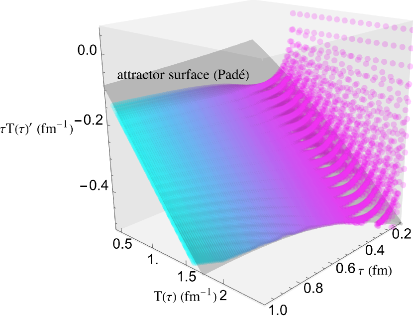
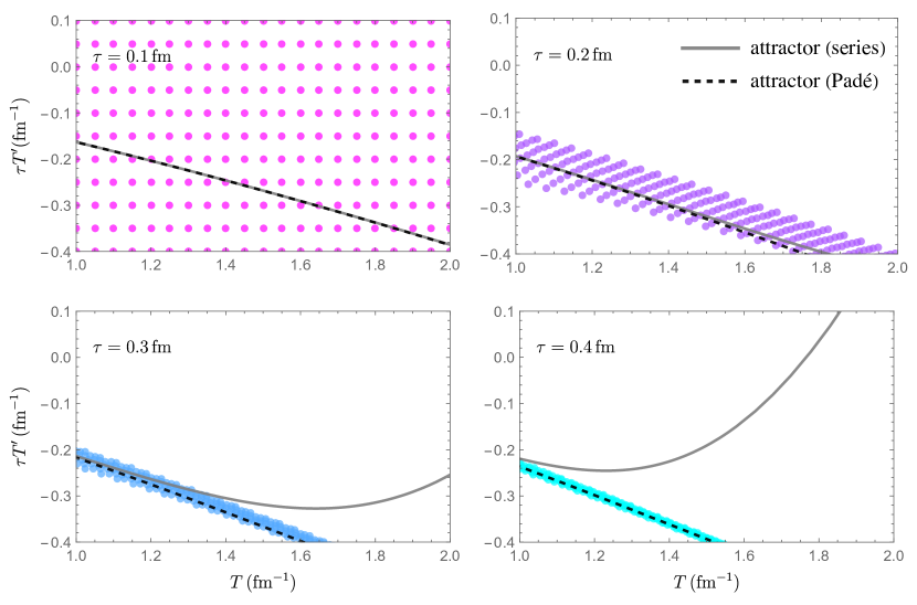
Figure 1: The left panel shows the early-time attractor in the 3D phase space $(\tau,T,\tau T^{\prime})$ with uniformly distributed initial conditions (points) at $\tau=0.1$ fm. The 2D attractor surface is obtained using Padé approximation of the series in Eqs. (5). The right panel are the snapshots of the 3D plot at different times, where the solid and dashed line represents the series solution and its Padé approximant respectively.

At late times, we expect the system to approach equilibrium in a way consistent with the original insights of Bjorken [1]. In that regime, solutions to Eqs. (3) can be represented in the form of transseries:

$$T(\tau) \sim\Lambda\left[(\Lambda\tau)^{-\frac{1}{3}}\left(1+\sum_{n=1}^{\infty}t_{n}^{(\infty)}(\Lambda\tau)^{-\frac{2n}{3}}\right)+C_{\infty}(\Lambda\tau)^{-\frac{2}{3}(1-\alpha^{2})}e^{-\frac{3}{2C_{\tau}}(\Lambda\tau)^{2/3}}\left(1+\mathcal{O}((\Lambda\tau)^{-\frac{2}{3}})\right)+\cdots\right],$$ (7a)

$$\mathcal{A}(\tau) \sim 8C_{\eta}(\Lambda\tau)^{-\frac{2}{3}}\left(1+\sum_{n=1}^{\infty}a_{n}^{(\infty)}(\Lambda\tau)^{-\frac{2n}{3}}\right)+C_{\infty}^{\prime}(\Lambda\tau)^{-\frac{1}{3}(1-3\alpha^{2})}e^{-\frac{3}{2C_{\tau}}(\Lambda\tau)^{2/3}}\left(1+\mathcal{O}((\Lambda\tau)^{-\frac{2}{3}})\right)+\cdots$$ (7b)

These are of the form of an asymptotic power series augmented by an infinite set of exponential transseries contributions, of which only the leading one is displayed above. The initial conditions are mapped to the dimensionful scale $\Lambda$ and the dimensionless integration constants $C_{\infty}$ and $C^{\prime}_{\infty}$. The first few coefficients of the late-time series $t_{n}^{(\infty)}$ and $a_{n}^{(\infty)}$ are given by

$$t^{(\infty)}_{1}=-\frac{2C_{\eta}}{3},\quad t^{(\infty)}_{2}=-\frac{2C_{\eta}C_{\tau}}{9},\quad\cdots$$ (8a)

$$a^{(\infty)}_{1}=\frac{2C_{\tau}}{3}(1+\alpha^{2}),\quad a^{(\infty)}_{2}=\frac{2C_{\tau}^{2}}{9}(4-\alpha^{2}+2\alpha^{4}),\quad\cdots$$ (8b)

Note that in the limit $C_{\tau}\to 0$ the leading and next-to-leading terms in Eqs. (7) reduce to their NS form, given in Eq. (4), upon substituting the coefficients in Eqs. (8). The power series appearing in Eqs. (7) have a vanishing radius of convergence and are best interpreted in the sense of asymptotic analysis — through optimal truncation or by Borel summation (see e.g. Refs. [16, 14]).

The description of the attractor presented above differs from the original formulation of Ref. [2] in that it uses proper time as the evolution parameter, rather than the dimensionless evolution variable $w\sim\tau T$. This is natural when the dynamic system possesses scales in addition to temperature, as will be discussed in Sec. III.

III The transverse perturbations

In the previous Section, we discussed an idealized description which was homogeneous in the transverse plane. While this idealization provides a useful first approximation for modeling the heavy-ion collisions at sufficiently high energies, it cannot account for physical observables which depend on the structure of the plasma in the transverse plane. In this Section, we relax this condition by considering additional fields which aim to model the transverse dynamics. These additional fields arise a perturbations of the fully-nonlinear hydrodynamic equations Eq. (1) around the attractor background.

III.1 The linearized equations

We will look for solutions that can be approximated by the boost-invariant and translation-invariant background solution discussed in Sec. II and a perturbation depending also on the transverse coordinates:

$$T(\tau,\bm{x})=T(\tau)+\delta T(\tau,\bm{x}),\quad{u^{\mu}}(\tau,\bm{x})=u^{\mu}+\delta{u^{\mu}}(\tau,\bm{x}),\quad{\pi^{\mu\nu}}(\tau,\bm{x})=\pi^{\mu\nu}(\tau)+\delta{\pi^{\mu\nu}}(\tau,\bm{x}),$$ (9)

where $\bm{x}=(x_{1},x_{2})$ labels the coordinates of the transverse plane. We shall always retain the argument $\bm{x}$ of the above quantities to distinguish the full ones from the background, which depends only on $\tau$ (and, as the only argument, is often suppressed). The background fields $T$ and $\pi^{\mu\nu}$ are taken to be on the attractor locus defined in Sec. II, and $u^{\mu}=(-1,\bm{0},0)$. Due to the assumed symmetries and the transversality condition $u^{\mu}\pi_{\mu\nu}=0$, the shear-stress tensor has only one independent background component (i.e., $\pi^{11}=\pi^{22}$) and three independent perturbation components (i.e., $\delta\pi^{11},\delta\pi^{22},\delta\pi^{12}$) that couple to the perturbation of hydrodynamic fields $\delta T$ and $\delta\bm{u}$. We also put $\delta\pi^{i\eta}=0$, which is consistent due to $\delta u^{\eta}=0$.

The perturbation fields can also be normalized by the background energy scale $T(\tau)$, i.e.,

$$\delta\hat{T}(\tau,\bm{x})=\frac{\delta T(\tau,\bm{x})}{T(\tau)},\quad\delta\hat{\pi}_{ij}(\tau,\bm{x})=\frac{\delta\pi_{ij}(\tau,\bm{x})}{C_{e}T(\tau)^{4}},$$ (10)

such that all six perturbation fields, denoted collectively by $\hat{\phi}(\tau,\bm{x})=(\hat{\delta}T,\delta u_{1},\delta u_{2},\hat{\delta}\pi_{12},\hat{\delta}\pi_{11},\hat{\delta}\pi_{22})$, are dimensionless. Since the background is independent of the transverse coordinates, it is also natural and convenient to introduce the Fourier transforms just for the perturbations:

$$\hat{\phi}(\tau,\bm{x})=\int\frac{d^{2}k}{(2\pi)^{2}}\ e^{i\bm{k}\cdot\bm{x}}{\hat{\phi}}(\tau,\bm{k}),$$ (11)

where we retain the argument $\bm{x}$ or $\bm{k}$ to distinguish perturbation fields $\hat{\phi}$ in different Fourier spaces.

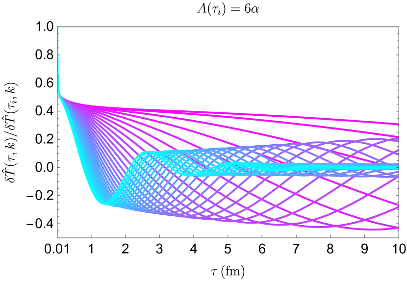
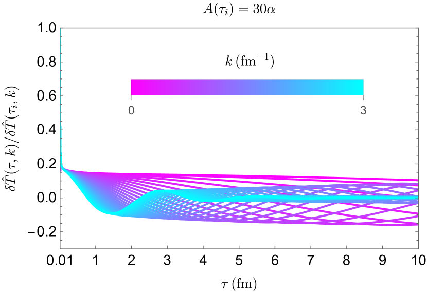
Figure 2: Evolution of Fourier modes with various values of $k$ between $0-3\,\text{fm}^{-1}$, with the background on the attractor, $\mathcal{A}(\tau_{i})=6\alpha$ (left) and off it, $\mathcal{A}(\tau_{i})=30\alpha$ (right). The initial time is $\tau_{i}=0.01$ fm.

Linearization of the full MIS equations (1) around an attractor solution leads to a system of six linear partial differential equations for the perturbations. For each value of $\bm{k}$ the set of six modes $\hat{\phi}(\tau,\bm{k})\equiv(\delta\hat{T},\delta u_{1},\delta u_{2},\delta\hat{\pi}_{12},\delta\hat{\pi}_{11},\delta\hat{\pi}_{22})$ satisfies a linear system of evolution equations which can be explicitly written as

$$4\left(\tau\partial_{\tau}+\frac{2\mathcal{A}}{9}\right)\delta\hat{T}+\frac{i(12+\mathcal{A})}{9}\tau k_{i}\delta u^{i}-\delta\hat{\pi}^{i}_{i} =0,$$ (12a)

$$\frac{i4}{3}\tau k_{i}\delta\hat{T}+\frac{1}{9}\left[(12+\mathcal{A})\tau\partial_{\tau}-4+\frac{8C_{\eta}}{C_{\tau}}+\left(\frac{7}{3}-\frac{\tau T}{C_{\tau}}\right)\mathcal{A}\right]\delta u_{i}+i\tau k^{j}\delta\hat{\pi}_{ij} =0,$$ (12b)

$$\frac{1}{9}\left(\frac{\tau T}{C_{\tau}}\mathcal{A}-\frac{32C_{\eta}}{C_{\tau}}\right)\delta_{ij}\delta\hat{T}+\frac{i4\tau}{27}\left[\left(\mathcal{A}-\frac{6C_{\eta}}{C_{\tau}}\right)\delta_{ij}k_{\ell}+\frac{9C_{\eta}}{C_{\tau}}(\delta_{i\ell}k_{j}+\delta_{j\ell}k_{i})\right]\delta u^{\ell}+\left(\tau\partial_{\tau}+\frac{\tau T}{C_{\tau}}+\frac{2\mathcal{A}}{9}\right)\delta\hat{\pi}_{ij} =0.$$ (12c)

Since modes with different $\bm{k}$ are decoupled at the linearized level, we omit the arguments $\tau$ and $\bm{k}$ unless needed.

It is straightforward to solve the system given in Eqs. (12) together with Eqs. (3) numerically for any given wave vector $k$. The most obvious consequence of such a calculation is the fact that modes with higher $k$ are damped more strongly than modes with low $k$, as illustrated in the left panel of Fig. 2. The origin of this phenomenon can be understood analytically, as will be discussed in Sec. III.2. Moreover, the perturbations starting away from the attractor are damped more significantly compared to perturbations starting on the attractor, as illustrated in the right panel of Fig. 2. This demonstrates the stability of the linearization around the attractor background.

III.2 Late-time behaviour of perturbations

In this Section we will try to understand analytically the late proper-time behaviour of the modes $\hat{\phi}$. The set of six ODEs describing the evolution of these modes can be analysed by standard asymptotic methods, although the complexity of this problem makes the calculation technically nontrivial.

For the purpose of calculating the asymptotics it is convenient to introduce the transverse divergence $\delta\theta(\tau,\bm{x})\equiv\partial_{i}\delta u^{i}$ and longitudinal vorticity $\delta\omega(\tau,\bm{x})\equiv\epsilon_{ij}\partial^{i}\delta u^{j}$ where $\epsilon_{ij}$ is the Levi-Civita symbol. In $\bm{k}$ space we will use the following dimensionless quantities, normalised by $k\equiv|\bm{k}|$:

$$\delta\hat{\theta}(\tau,\bm{k})=\frac{\delta{\theta}(\tau,\bm{k})}{k}=i\hat{k}_{i}\delta u^{i}(\tau,\bm{k}),\quad\delta\hat{\omega}(\tau,\bm{k})=\frac{\delta{\omega}(\tau,\bm{k})}{k}=i\epsilon_{ij}\hat{k}^{i}\delta u^{j}(\tau,\bm{k}),$$ (13)

where $\hat{k}_{i}\equiv k_{i}/k$. For such a choice of variables, the linear system of evolution equations reads

$$4\left(\tau\partial_{\tau}+\frac{2\mathcal{A}}{9}\right)\delta\hat{T}+\frac{(12+\mathcal{A})}{9}\tau k\delta\hat{\theta}-\delta\hat{\pi}^{i}_{i} =0,$$ (14a)

$$-\frac{4}{3}k^{2}\delta\hat{T}+\frac{1}{9\tau}\left[(12+\mathcal{A})\tau\partial_{\tau}-4+\frac{8C_{\eta}}{C_{\tau}}+\left(\frac{7}{3}-\frac{\tau T}{C_{\tau}}\right)\mathcal{A}\right]k\delta\hat{\theta}-k_{i}k_{j}\delta\hat{\pi}^{ij} =0,$$ (14b)

$$\frac{1}{9\tau}\left[(12+\mathcal{A})\tau\partial_{\tau}-4+\frac{8C_{\eta}}{C_{\tau}}+\left(\frac{7}{3}-\frac{\tau T}{C_{\tau}}\right)\mathcal{A}\right]k\delta\hat{\omega}-\epsilon_{ij}k^{j}k^{\ell}\delta\hat{\pi}^{i}_{\ell} =0,$$ (14c)

$$\frac{1}{9}\left(\frac{\tau T}{C_{\tau}}\mathcal{A}-\frac{32C_{\eta}}{C_{\tau}}\right)\delta_{ij}\delta\hat{T}+\frac{4\tau}{27k}\left[\frac{18C_{\eta}}{C_{\tau}}k_{i}k_{j}+\left(\mathcal{A}-\frac{6C_{\eta}}{C_{\tau}}\right)k^{2}\delta_{ij}\right]\delta\hat{\theta}$$

$$-\frac{4C_{\eta}(k_{i}\epsilon_{j\ell}+k_{j}\epsilon_{i\ell})k^{\ell}\tau}{3C_{\tau}k}\delta\hat{\omega}+\left(\tau\partial_{\tau}+\frac{\tau T}{C_{\tau}}+\frac{2\mathcal{A}}{9}\right)\delta\hat{\pi}_{ij} =0.$$ (14d)

At this juncture, one way to proceed is to rewrite this system in terms of higher-order ODEs; remarkably, it can be written as a set of three second-order ODEs for $\delta\hat{T},\delta\hat{\theta},\delta\hat{\omega}$ — they are given in Appendix A. Two of these equations couple $\delta\hat{T}$ and $\delta\hat{\theta}$, while the third involves $\delta\hat{\omega}$ alone. The two coupled equations can be combined into a fourth order ODE for $\delta\hat{T}$, whose asymptotic behaviour can be studied by standard methods (see e.g. Ref [17]). This is in principle straightforward, but is somewhat challenging in practice due to the complexity of the coefficients which appear in this equation. Alternatively, one can analyse the system of six first order ODEs directly using the methods developed in Ref. [18]. Both approaches gives rise to the same late-time asymptotic solutions whose leading terms take the form:

$$\delta\hat{T} =\sum_{i=1}^{4}C_{i}(\Lambda\tau)^{\beta_{i}}e^{-i\omega_{i}\tau-A_{i}(\Lambda\tau)^{2/3}},$$ (15a)

$$\delta\hat{\theta} =\sum_{i=1}^{4}C^{\prime}_{i}(\Lambda\tau)^{\beta^{\prime}_{i}}e^{-i\omega_{i}\tau-A_{i}(\Lambda\tau)^{2/3}},$$ (15b)

$$\delta\hat{\omega} =\sum_{i=5}^{6}C_{i}(\Lambda\tau)^{\beta_{i}}e^{-i\omega_{i}\tau-A_{i}(\Lambda\tau)^{2/3}}.$$ (15c)

The initial conditions are accounted for by the amplitudes $C_{1},\dots,C_{6}$ and $C_{1}^{\prime},\dots,C_{4}^{\prime}$. The primed integration constants are related to the unprimed ones by the relations

$$C_{1}^{\prime}=3ic_{\alpha}C_{1},\quad C_{2}^{\prime}=-3ic_{\alpha}C_{2},\quad C_{3}^{\prime}=-\frac{(1-3\alpha^{2})\Lambda}{2\alpha^{2}k}C_{3},\quad C_{4}^{\prime}=\frac{\Lambda}{c_{\alpha}^{2}C_{\tau}k}C_{4},$$ (16)

so that only the unprimed integration constants $C_{1},\dots,C_{6}$ are independent. Recall also that each of the perturbations appearing above depends on the wave vector $\bm{k}$, and so do the coefficients $C_{1},\dots,C_{6}$.

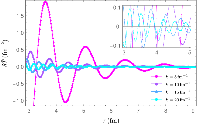
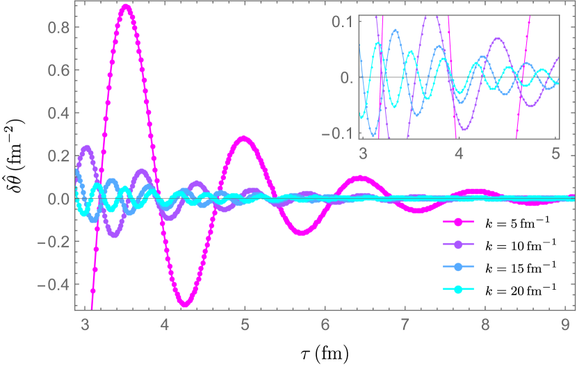
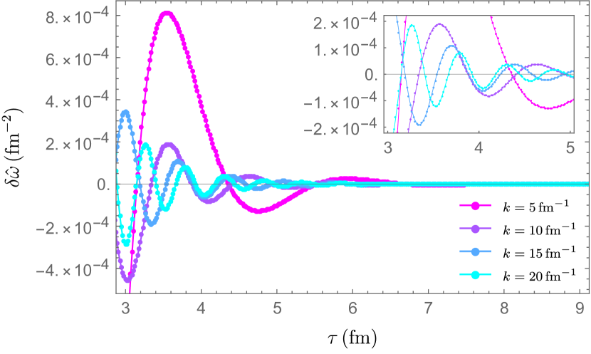
Figure 3: These figures show the analytic late-time asymptotic solution (solid line) and the numerical results (discrete points) for various values of wave vector $k$. They were obtained by fitting the amplitudes $C_{i}$. The inset plots are provided to give a better view of the small-$\tau$ region.

The remaining quantities appearing in Eqs. (15) above are determined in terms of the parameters of the theory and do not depend on the initial state. The parameters appearing in the exponentials are given by

$$A_{1}=A_{2}=\frac{\alpha^{2}}{C_{\tau}c_{\alpha}^{2}},\quad A_{3}=\frac{3}{2C_{\tau}},\quad A_{4}=\frac{1}{2C_{\tau}c_{\alpha}^{2}},\quad A_{5}=A_{6}=\frac{3}{4C_{\tau}},$$

$$\omega_{1}=-\omega_{2}=c_{\alpha}k\left[1+\frac{2\alpha^{2}}{3c_{\alpha}^{2}}\left(2C_{\tau}(1-\alpha^{2})-\frac{(1+\alpha^{2})\Lambda^{2}}{C_{\tau}^{2}c_{\alpha}^{4}k^{2}}\right)(\Lambda\tau)^{-2/3}\right],\quad\omega_{3}=\omega_{4}=0,$$

$$\omega_{5}=-\omega_{6}=\alpha k\left[1-\left(C_{\tau}\alpha^{2}+\frac{3\Lambda^{2}}{8C_{\tau}^{2}\alpha^{2}k^{2}}\right)(\Lambda\tau)^{-2/3}\right],$$ (17)

where $c_{\alpha}=\sqrt{(1+4\alpha^{2})/3}$ is the modified (asymptotic) speed of sound. The constant coefficients $A_{i}$ are the leading contributions to eigenvalues of the coupled linear equations describing perturbations around the attractor. They are real, positive and independent of the wave vectors $k$, implying stability of the attractor against transverse perturbations regardless of their scales. Note that the quantities $\omega_{1}=-\omega_{2}$ and $\omega_{5}=-\omega_{6}$ are actually functions of $\tau$, which also have a nontrivial dependence on the wave vectors $k$. At late times these quantities approach frequencies of oscillation which become harmonic in that domain.

The coefficients appearing in the power-law factors in Eqs. (15) are given by

$$\beta_{1}=\beta_{2}=\beta^{\prime}_{1}=\beta^{\prime}_{2}=\frac{1}{54c_{\alpha}^{4}}\left(1+8\alpha^{2}+64\alpha^{4}+32\alpha^{6}+\frac{4\alpha^{2}\Lambda^{2}}{C_{\tau}^{3}c_{\alpha}^{4}k^{2}}\right),\quad\beta_{3}=\beta^{\prime}_{3}+1=-\frac{2}{3}(1-\alpha^{2}),$$

$$\beta_{4}=\beta^{\prime}_{4}+\frac{1}{3}=\frac{2\alpha^{2}}{27c_{\alpha}^{4}}\left(1-16\alpha^{2}-\frac{2\Lambda^{2}}{C_{\tau}^{3}c_{\alpha}^{4}k^{2}}\right),\quad\beta_{5}=\beta_{6}=\frac{1}{6}(1+2\alpha^{2}),$$ (18)

A key point which follows from these relations is the suppression of modes with large $k$ relative to modes with smaller values of $k$. This fact was already noted in the numerical solutions discussed in Sec. III.1, but the asymptotic formulae Eqs. (15) in conjunction with Eq. (18) reveal the precise form of this suppression. Note also that the solution labelled by $i=3$ reproduces the transseries solution describing the homogeneous background (with the integration constant independent of $k$ in that case).

This highly nontrivial structure reproduces the behaviour seen in numerical simulations very accurately. At late time, the dominant asymptotic solutions for $\delta\hat{T}$ and $\delta\hat{\theta}$ are those which are least damped, i.e. with the smallest value of $A_{i}$. For the $\mathcal{N}=4$ supersymmetric Yang-Mills theory these are terms labeled by $i=1,2$ in the solutions of Eqs. (15). These formulae then capture only the leading exponential behaviour, but still give an excellent account of the numerical solutions, as illustrated in Fig. 3. It is also quite interesting to compare these results with the asymptotics of Navier-Stokes theory, as well as with the case of perfect fluids. This is discussed in Appendix B.

To summarise, at late times the characteristics of the initial state are mapped to the scale $\Lambda$ and dimensionless amplitudes $C_{1}(k)$ — $C_{6}(k)$ which carry information about the structure of the initial data in the transverse plane. These numbers can be matched to a given numerical solution. All physical observables can be expressed in terms of this asymptotic data, in manner described explicitly in the following Section.

III.3 Spacetime evolution of QGP

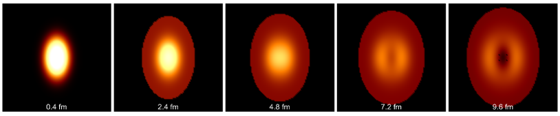
Figure 4: The evolution of temperature profile in the transverse plane for different at different instants of proper time (shown at the bottom of each image). The initial conditions assume the nuclear radius of $6.62$ fm (corresponding to lead). The impact parameter was taken to be $b=6$ fm. The dimensions of the region covered by the images are $60$ fm by $60$ fm.

The initial state resulting from a heavy ion collision can described by providing values of all the fields at the initial proper time as functions of the coordinates in the transverse plane. This initial data can be equivalently represented in terms of the Fourier modes $\hat{\phi}$ at the initial time. Realistic initial conditions are superpositions of infinitely many Fourier modes, but due to the strong damping of modes with high $k$, one can approximate the initial state by neglecting modes corresponding to large wave vectors. In practice, one needs to evaluate the initial conditions on a finite grid in the transverse plane, calculate the Fourier transform, evolve the modes by solving Eqs. (12) and then compute the inverse Fourier transform to reconstruct the spacetime history of the QGP. The problem can thus be described by a finite set of modes which encode the transverse structure of the initial state. The procedure can be made highly efficient by applying the Fast Fourier Transform (see e.g. Ref. [19]).

In our pilot study we consider a computational domain which is a $60$ fm by $60$ fm square region in the transverse plane, described by a regular grid of $100$ by $100$ points. A corresponding (conjugate) grid is then constructed in $\bm{k}$-space — this also introduces a cutoff on large $k$. We have implemented the steps outlined above for the case of very simple initial conditions which assume $\delta T$ in the form of a Gaussian distribution in transverse coordinates with a specified impact parameter $b$. The remaining fields are taken to vanish at the initial time, which is a natural choice at least in the case of the transverse velocity perturbation. This leads to results shown Fig. 4. The data generated this way was also used to obtain some more quantitative results described in the following Section. One can of course apply this approach to initial states generated in other ways, such as events generated using Glauber Monte-Carlo.

IV QGP Physics

In this paper we will not undertake any systematic studies aiming to establish which physical effects are captured by the set of approximations which we described here. However, in this Section we would like to emphasise that all such effects are encoded in the exponentially damped contributions appearing in Eqs. (15). To this end, we will describe some quantitative analysis of the numerical calculation described in Sec. III.3.

IV.1 Transverse anisotropy

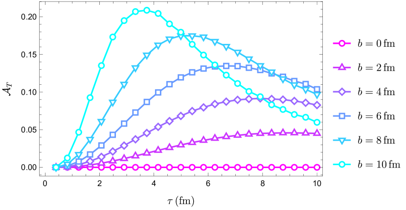
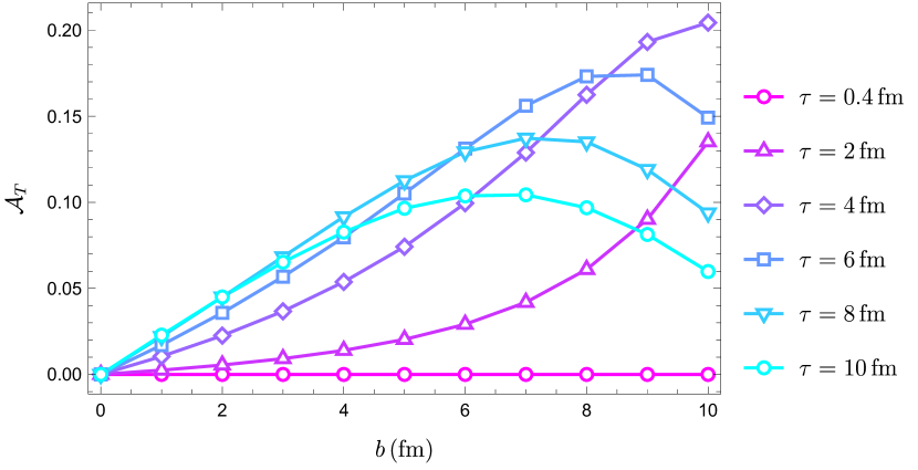
Figure 5: The dependence of transverse anisotropy $\mathcal{A}_{T}$ on $\tau$ for different values of $b$ (left) and on $b$ for different values of $\tau$. The initial conditions for the perturbations are set at $\tau=0.4\mathrm{fm}$ and are otherwise the same as those used to produce Fig. 4.

As a first indication that we can at least qualitatively account for some nontrivial physics related to the transverse expansion, we would like to address the issue of collectivity at the level of elliptic flow. Similarly to the pressure anisotropy which characterizes the difference between the longitudinal and two transverse stress tensor components, one can introduce the notion of transverse anisotropy (also referred to the momentum anisotropy), which characterizes the difference between the two transverse diagonal components themselves. This anisotropy is nonvanishing when rotational invariance is broken and is approximately twice as large as the flow harmonic coefficient $v_{2}$ which serves as an important indicator of collective flow in heavy-ion collision experiments[20, 21, 22]. The leading terms in the transverse anisotropy are

$$\mathcal{A}_{T}(\tau)\equiv\frac{\langle{T_{11}-T_{22}}\rangle_{\perp}}{\langle{T_{11}+T_{22}}\rangle_{\perp}}=\frac{12\langle{\delta u_{1}^{2}-\delta u_{2}^{2}}\rangle_{\perp}+9\langle{\delta\hat{\pi}_{11}-\delta\hat{\pi}_{22}}\rangle_{\perp}}{2(3+\mathcal{A})},$$ (19)

where $\langle{\dots}\rangle_{\perp}=\int dx_{1}dx_{2}(\dots)/\int dx_{1}dx_{2}$ denotes the spacial average over the region occupied by the QGP in the transverse plane at a given instant of proper time. To calculate this quantity it is necessary to determine the transverse extent of the fluid. Since the background is homogeneous in the transverse plane, the boundary of the plasma drop is defined by the perturbation. Due to the finite resolution of the calculation, this means in practice that this boundary is taken to be the locus where the energy density deviates from the value at the periphery of the computational domain. The outcomes of this computation are illustrated in Fig. 5. Note also that the finiteness of the freeze-out time $\tau_{f}$ implies a finite spacial extent of the QGP drop.

IV.2 Freeze-out

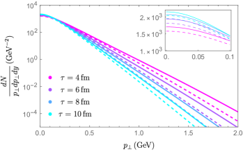
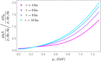
Figure 6: The left panel shows the transverse momentum dependence of pion distribution without and with perturbations (represented by dashed and solid lines), while the right panel shows the ratio of the perturbative contribution and the background.

The numerical solutions discussed in Sec. III show that at asymptotically late times the modes representing the perturbations are damped away and eventually the system follows the Bjorken background solution. The QGP never reaches that stage however due to hadronization: at some time the system described by the hydrodynamic variables is converted into a stream of hadrons. To calculate their distribution one needs to capture the fine details of the flow during the freeze-out epoch, when the hydrodynamic fields are converted into a set of outgoing particles. Within the linearization framework discussed here it is reasonable to model freeze-out by defining a single instant of proper time $\tau_{f}=\tau_{f}(\tau)$ which is independent of the transverse coordinates and only set by the homogeneous background, the corrections to which are beyond the linear approximation we consider here.

In heavy-ion collision experiments the observables refer to hadronized particles whose momentum distribution is given by the well-known Cooper–Frye formula [23]. For the Bjorken background $u^{\mu}=(\cosh\eta,\bm{0},\sinh\eta)$ with $\eta$ being the pseudo-rapidity of the fluid, and a given particle species with mass $m$ and momentum $p^{\mu}=(m_{\perp}\cosh y,\bm{p}_{\perp},m_{\perp}\sinh y)$, where $m_{\perp}=\sqrt{m^{2}+\bm{p}_{\perp}^{2}}$, and $y$ is the kinematic rapidity of the particle, the momentum distribution of particles created on the freeze-out surface is given by

$$\frac{dN_{\rm B}}{p_{\perp}dp_{\perp}d\phi dy}=\frac{1}{(2\pi)^{3}}\int d^{3}\sigma_{\mu}p^{\mu}f(x,p)=\frac{m_{\perp}\tau_{f}R^{2}}{8\pi^{2}}F_{0},\quad F_{0}=2K_{1}(\hat{m}_{\perp})+\frac{1}{12}\left[\hat{p}_{\perp}^{2}K_{1}(\hat{m}_{\perp})-2\hat{m}_{\perp}K_{2}(\hat{m}_{\perp})\right]\mathcal{A}$$ (20)

where $\hat{p}_{\perp}\equiv p_{\perp}/T\equiv|\bm{p}_{\perp}|/T$, $\hat{m}_{\perp}\equiv m_{\perp}/T$, $d^{3}\sigma_{\mu}=(\cosh\eta,\bm{0},-\sinh\eta)\tau_{f}d\eta d^{2}x$ is the area element of the freeze-out surface, $f(x,p)=e^{u\cdot\hat{p}}(1+\epsilon_{\mu\nu}\hat{p}^{\mu}\hat{p}^{\nu})$, with $\epsilon_{\mu\nu}=\pi_{\mu\nu}/2(\mathcal{E}+p)$, is the non-equilibrium phase space distribution for classical particle, $R$ is the transverse radius cutoff for the flow and $K_{n}(x)$ is the Bessel function of the second kind. At large $\hat{p}_{\perp}$, $F_{0}\sim\frac{\sqrt{2\pi}}{24}\mathcal{A}\,\hat{p}_{\perp}^{3/2}e^{-\hat{p}_{\perp}}$ (cf. the ideal limit where $F_{0}\sim\sqrt{2\pi}\hat{p}_{\perp}^{-1/2}e^{-\hat{p}_{\perp}}$) and thus Eq. (20) behaves like $\hat{p}_{\perp}^{5/2}e^{-\hat{p}_{\perp}}$. The ratio of the dissipative and ideal parts in Eq. (20) is asymptotically $\mathcal{A}\,\hat{p}_{\perp}^{2}/24$, which, at late time (NS limit), sets the maximum value of $p_{\perp}\sim\sqrt{3/C_{\eta}}\Lambda~{}(\sim 1-2$ GeV) where the hydrodynamic description breaks down. Indeed, Eq. (20) reduces to its NS limit by substituting Eq. (4b) [24].

The correction $\Delta N$ due to the contribution of the linearized perturbations up to quadratic order is given by

$$\frac{d\Delta N}{p_{\perp}dp_{\perp}d\phi dy}=\frac{m_{\perp}\tau_{f}R^{2}}{8\pi^{2}}\Big{[}F_{1}\langle{\delta\hat{T}}\rangle_{\perp}+F_{2}\,\hat{p}_{\perp}^{i}\langle{\delta u_{i}}\rangle_{\perp}+F_{3}\,\hat{p}_{\perp}^{i}\hat{p}_{\perp}^{j}\langle{\delta\hat{\pi}_{ij}}\rangle_{\perp}+F_{11}\langle{\delta\hat{T}\delta\hat{T}}\rangle_{\perp}+F_{12}\,\hat{p}_{\perp}^{i}\langle{\delta u_{i}\delta\hat{T}}\rangle_{\perp}\\ +F_{13}\,\hat{p}_{\perp}^{i}\hat{p}_{\perp}^{j}\langle{\delta\hat{\pi}_{ij}\delta\hat{T}}\rangle_{\perp}+F_{22}\,\hat{p}_{\perp}^{i}\hat{p}_{\perp}^{j}\langle{\delta u_{i}\delta u_{j}}\rangle_{\perp}+F_{23}\,\hat{p}_{\perp}^{i}\hat{p}_{\perp}^{j}\hat{p}_{\perp}^{k}\langle{\delta\hat{\pi}_{ij}\delta u_{k}}\rangle_{\perp}\Big{]},$$ (21)

where $\hat{p}_{\perp}^{1}=\hat{p}_{\perp}\cos\phi$, $\hat{p}_{\perp}^{2}=\hat{p}_{\perp}\sin\phi$, and

$$F_{1}=\hat{m}_{\perp}\left[K_{0}(\hat{m}_{\perp})+K_{2}(\hat{m}_{\perp})\right]-\frac{1}{6}\left[(\hat{m}_{\perp}^{3}+3\hat{p}_{\perp}^{2})K_{1}(\hat{m}_{\perp})+3\hat{m}_{\perp}(\hat{m}_{\perp}-2)K_{2}(\hat{m}_{\perp})\right]\mathcal{A},\quad F_{2}=2F_{22}=F_{0},$$

$$F_{3}=F_{23}=\frac{3}{4}K_{1}(\hat{m}_{\perp}),\quad F_{13}=\frac{3}{4}\left[\hat{m}_{\perp}K_{0}(\hat{m}_{\perp})-5K_{1}(\hat{m}_{\perp})\right],\quad F_{11}=-\hat{m}_{\perp}K_{0}(\hat{m}_{\perp})+\hat{m}_{\perp}^{2}K_{1}(\hat{m}_{\perp})$$

$$+\frac{1}{24}\left[-14\hat{m}_{\perp}\hat{p}_{\perp}^{2}K_{0}(\hat{m}_{\perp})+2(14\hat{m}_{\perp}^{2}+42\hat{p}_{\perp}^{2}+\hat{m}_{\perp}^{2}\hat{p}_{\perp}^{2})K_{1}(\hat{m}_{\perp})-(\hat{m}_{\perp}^{3}+12\hat{p}_{\perp}^{2})K_{2}(\hat{m}_{\perp})-\hat{m}_{\perp}^{3}K_{4}(\hat{m}_{\perp})\right]\mathcal{A},$$

$$F_{12}=2\hat{m}_{\perp}K_{0}(\hat{m}_{\perp})+\frac{1}{24}\left[\hat{m}_{\perp}(16+\hat{p}_{\perp}^{2})K_{0}(\hat{m}_{\perp})+2(16-2\hat{m}_{\perp}^{2}-7\hat{p}_{\perp}^{2})K_{1}(\hat{m}_{\perp})+\hat{m}_{\perp}\hat{p}_{\perp}^{2}K_{2}(\hat{m}_{\perp})\right]\mathcal{A}.$$ (22)

At large $\hat{p}_{\perp}$, Eq. (21) is asymptotically dominated by terms $\langle{\delta\hat{T}\delta\hat{T}}\rangle_{\perp}$ and $\langle{\delta u_{i}\delta u_{j}}\rangle_{\perp}$, with coefficients $F_{11}\sim F_{22}\hat{p}_{\perp}^{2}\sim\frac{\sqrt{2\pi}}{24}\mathcal{A}\,{\hat{p}_{\perp}}^{7/2}e^{-\hat{p}_{\perp}}$, so that Eq. (21) behaves as $\hat{p}_{\perp}^{9/2}e^{-\hat{p}_{\perp}}$. Comparing this to the asymptotic behavior of Eq. (20) we infer that the transverse perturbation is small relative to the background only as long as $\hat{p}_{\perp}\lesssim 1$ (see also the right panel of Fig. 6). When $\hat{p}_{\perp}$ becomes of order one, it would be natural to resum the series in Eq. (21) using a Padé approximant. Nevertheless, we note that although the large $p_{\perp}$ behavior is nonperturbative, its the magnitude is also negligible compared to the lower $p_{\perp}$ behavior. The distribution of total particle number $N=N_{\rm B}+\Delta N$ obtained by adding Eqs. (20) and (21) is shown in the left panel of Fig. 6.

The dependence of the multiplicity on both $p_{\perp}$ and $\phi$ is shown in Fig. 7. In particular, we compare the dependence of the multiplicity distribution on $\phi$ for two different impact parameters $b$. The distribution resulting from a central collision ($b=0$) does not depend on $\phi$, as one would expect, due to the isotropy of the system. On the other hand, the right panel clearly shows the dependence on the asymuthal angle for a noncentral collision. This demonstrates the importance of the contribution from perturbations in both magnitude of particle yields and angular distribution in transverse plane.

V Outlook

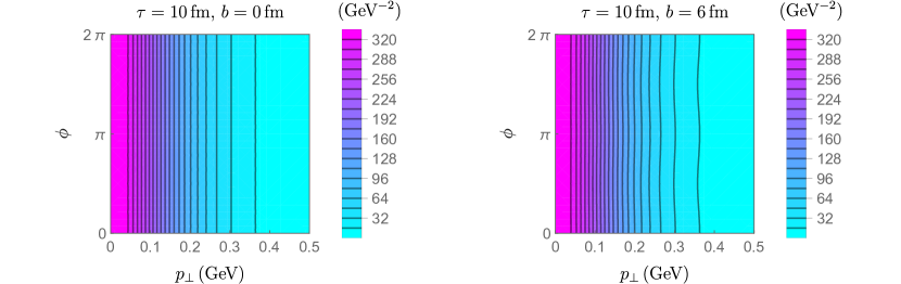
Figure 7: This figure shows the 2D contour plot of the multiplicity distribution $dN/p_{\perp}dp_{\perp}d\phi dy$ at $\tau=10$ fm with different impact parameters, i.e., $b=0$ fm (left) and $b=6$ fm (right) respectively.

Despite the radical simplifications made, the original Bjorken model provided a very useful analytic formula describing the dynamics of the energy density and has lead to many important insights. The incorporation of viscous effects and higher orders in the large proper time expansion retained some of the simplicity of the original Bjorken model, allowing for approximate analytic calculations and significantly simplifying numerical computations. However, the stringent symmetry requirements — boost invariance and homogeneity in the transverse plane – placed severe limits on how much of the physics could be described by such models. In this article we have aimed to balance simplicity with the ability to capture more of the interesting physics of QGP. To this end, we have partially relaxed the symmetry requirements, insisting only on longitudinal boost invariance while incorporating transverse dynamics by linearizing around a boost-invariant attractor background, characterised by a choice of the initial temperature. In this way we have formulated a description which goes beyond toy models, but still allows some analytic insights which can be extracted by applying known asymptotic techniques.

The initial state is encoded in the initial conditions for the Fourier modes of the transverse perturbations and the initial temperature of the attractor background. The evolution equations map this initial-state information into a set of six exponentially suppressed scale-dependent amplitudes (transseries coefficients) and a scale $\Lambda$. From the perspective of modern asymptotic analysis our work shows that the dynamics of QGP created in heavy-ion collision experiments provides a physical situation where the exponentially suppressed corrections to asymptotic power series solutions carry almost all the information which is actually detected in experiments. We have shown how these exponential corrections are translated into the physics post-freeze-out.

Aside from providing a clear, semi-analytic picture of QGP evolution, our approach can be implemented numerically in a very straightforward and efficient fashion, since it relies on the discrete Fourier transforms and solving systems of coupled linear ODEs. The details of the initial state can be incorporated scale by scale in a controlled way: to account for finer detail of the initial state we can increase the number of modes in the calculation whose computational complexity then scales linearly. Apart from the conceptual utility, our approach can thus be used as a laboratory for studying models of the initial state, as well as novel characterisations of fluid behaviour [25, 26]. Our model can also be extended in a number of ways; two most prominent are the description of jets [27, 28, 29, 30], and the incorporation of noise [31, 32, 33, 34, 35, 36]. We hope to return to these matters in the future.

We have provided some examples which demonstrate that our approach is able to reproduce basic features which rely on an effective description of the transverse dynamics. It is however not yet clear which physical effects are captured by this model, and which require a fully-nonlinear treatment. In our pilot study we have considered the buildup of elliptic flow and have found results consistent with earlier work which relied on solving the fully-nonlinear problem. It would be very interesting to better understand the limitations of our approach.

VI Acknowledgements

It is a pleasure to thank V. Ambrus, L. Du, W. Florkowski and S. Mrówczyński, M. Stephanov for helpful discussions. This work was supported by the National Science Centre, Poland, under Grant No. 2021/41/B/ST2/02909. The authors would also like to thank the Isaac Newton Institute for Mathematical Sciences, Cambridge, for support and hospitality during the program “Applicable resurgent asymptotics: towards a universal theory” supported by EPSRC Grant No. EP/R014604/1.

VII Appendix

Appendix A Linearized ODEs

The six first-order linear differential equations in (14) can be written as three second-order linear differential equations by eliminating the variables $\pi_{ij}$, the resulting equations take the form

$$\partial^{2}_{\tau}\delta\hat{T}+P^{(1)}_{TT}\partial_{\tau}\delta\hat{T}(\tau)+P^{(1)}_{T\theta}\partial_{\tau}\delta\hat{\theta}+P^{(0)}_{TT}\delta\hat{T}+P^{(0)}_{T\theta}\delta\hat{\theta}=0,$$ (23a)

$$\partial^{2}_{\tau}\delta\hat{\theta}+P^{(1)}_{\theta T}\partial_{\tau}\delta\hat{T}+P^{(1)}_{\theta\theta}\partial_{\tau}\delta\hat{\theta}+P^{(0)}_{\theta T}\delta\hat{T}+P^{(0)}_{\theta\theta}\delta\hat{\theta}=0,$$ (23b)

$$\partial^{2}_{\tau}\delta\hat{\omega}+P^{(1)}_{\omega\omega}\partial_{\tau}\delta\hat{\omega}+P^{(0)}_{\omega\omega}\delta\hat{\omega}=0,$$ (23c)

with the matrix coefficients $P_{AB}^{(n)}$ where $A,B=T,\theta,\omega$ and $(n)$ denotes the differentiation order of the corresponding term:

$$P^{(1)}_{TT}=\frac{9(1+w)+4\mathcal{A}}{9\tau},\quad P^{(1)}_{T\theta}=\frac{k(12+\mathcal{A})}{36},\quad P^{(0)}_{TT}=\frac{-288\alpha^{2}+\left(45w+8\mathcal{A}+36\tau\partial_{\tau}\right)\mathcal{A}}{162\tau^{2}},$$

$$P^{(0)}_{T\theta}=\frac{k}{324\tau}\left[36(3+2\alpha^{2}+3w)+(57+9w+2\mathcal{A}+9\tau\partial_{\tau})\mathcal{A}\right],\quad P^{(1)}_{\theta T}=\frac{12k}{12+\mathcal{A}},$$

$$P^{(1)}_{\theta\theta}=P^{(1)}_{\omega\omega}=\frac{-36(1-2\alpha^{2}-3w)+(45+2\mathcal{A}+9\tau\partial_{\tau})\mathcal{A}}{9(12+\mathcal{A})\tau},\quad P^{(0)}_{\theta T}=-\frac{k[12(8\alpha^{2}+3w)+\left(8-3w\right)\mathcal{A}]}{3(12+\mathcal{A})\tau},$$

$$P^{(0)}_{\theta\theta}=\frac{1}{27(12+\mathcal{A})\tau^{2}}\Big{\{}108\left[(1-2\alpha^{2})(1-w)+4\alpha^{2}k^{2}\tau^{2}\right]$$

$$+\left[-3(29-16\alpha^{2}-12k^{2}\tau^{2}+9w\tau\partial_{\tau}\ln T)+(7-3w)(9w+2\mathcal{A}+9\tau\partial_{\tau})\right]\mathcal{A}\Big{\}},$$

$$P^{(0)}_{\omega\omega}=\frac{1}{27(12+\mathcal{A})\tau^{2}}\Big{\{}108\left[(1-2\alpha^{2})(1-w)+3\alpha^{2}k^{2}\tau^{2}\right]$$

$$+\left[-3(29-16\alpha^{2}+9w\tau\partial_{\tau}\ln T)+(7-3w)\left(9w+2\mathcal{A}+9\tau\partial_{\tau}\right)\right]\mathcal{A}\Big{\}},$$ (24)

where $w\equiv\tau T/C_{\tau}$. One immediately notices that the equation for vorticity $\delta\omega$ in Eq.  (23) decouples from the other two equations. Given a solution to these equations, one can recover the independent shear-stress tensor components algebraically.

Substituting Eq. (7) into Eqs. (23), and taking $C_{\tau}=0$ and $C_{\eta}/\tau T\ll 1$, Eqs. (23) reduces to its the NS limit as those presented also in Ref. [37]:

$$\partial_{\tau}\delta\hat{T}+\frac{k}{3}\left(1+\frac{4C_{\eta}}{3\tau T}\right)\delta\hat{\theta}=0,$$ (25a)

$$\partial_{\tau}\delta\hat{\theta}-\frac{1}{3\tau}\left(1-\frac{4C_{\eta}k^{2}\tau}{T}\right)\delta\hat{\theta}-k\left(1+\frac{4C_{\eta}}{3\tau T}\right)\delta\hat{T}=0,$$ (25b)

$$\partial_{\tau}\delta\hat{\omega}-\frac{1}{3\tau}\left(1-\frac{3C_{\eta}k^{2}\tau}{T}\right)\delta\hat{\omega}=0.$$ (25c)

The equation for the ideal fluid is simply obtained by setting $C_{\eta}=0$ in Eqs. (25).

Appendix B The late-time asymptotic solutions in Navier-Stokes and ideal limits

The asymptotic solutions shall be obtained using Eqs. (14). In the NS limit, $C_{\tau}=0$, we find

$$\delta\hat{T}_{\rm NS} =D_{1}(\Lambda\tau)^{-\beta_{4}^{\rm NS}}\exp\left[-\frac{C_{\eta}k^{2}}{\Lambda^{2}}(\Lambda\tau)^{4/3}+\frac{3}{8C_{\eta}}(\Lambda\tau)^{2/3}\right]+D_{2}(\Lambda\tau)^{\beta_{4}^{\rm NS}}\exp\left[-\frac{3}{8C_{\eta}}(\Lambda\tau)^{2/3}\right],$$ (26a)

$$\delta\hat{\theta}_{\rm NS} =D_{1}^{\prime}(\Lambda\tau)^{-\beta_{4}^{\rm NS}+\frac{1}{3}}\exp\left[-\frac{C_{\eta}k^{2}}{\Lambda^{2}}(\Lambda\tau)^{4/3}+\frac{3}{8C_{\eta}}(\Lambda\tau)^{2/3}\right]+D_{2}^{\prime}(\Lambda\tau)^{\beta_{4}^{\rm NS}-\frac{1}{3}}\exp\left[-\frac{3}{8C_{\eta}}(\Lambda\tau)^{2/3}\right],$$ (26b)

$$\delta\hat{\omega}_{\rm NS} =D_{3}(\Lambda\tau)^{1/3}\exp\left[-\frac{3C_{\eta}k^{2}}{4\Lambda^{2}}(\Lambda\tau)^{4/3}+\frac{8C_{\eta}}{3}(\Lambda\tau)^{-2/3}\right],$$ (26c)

where $\beta_{4}^{\rm NS}=-\frac{2}{3}-\frac{3\Lambda^{2}}{64C_{\eta}^{3}k^{2}}$ and $D$’s are integration constants.

In the ideal limit, $C_{\tau}=C_{\eta}=0$, from Eqs. (25) with $C_{\eta}=0$ one immediately obtains, with $E$’s being integration constants, that

$$\delta\hat{T}_{\rm I}=(\Lambda\tau)^{1/6}\left(E_{1}e^{-\frac{i}{\sqrt{3}}k\tau}+E_{2}e^{\frac{i}{\sqrt{3}}k\tau}\right),\quad\delta\hat{\theta}_{\rm I}=i\sqrt{3}(\Lambda\tau)^{1/6}\left(E_{1}e^{-\frac{i}{\sqrt{3}}k\tau}-E_{2}e^{\frac{i}{\sqrt{3}}k\tau}\right),\quad\delta\hat{\omega}_{\rm I}=E_{3}(\Lambda\tau)^{1/3}.$$ (27)

References

- [1] J.D. Bjorken, Highly Relativistic Nucleus-Nucleus Collisions: The Central Rapidity Region, Phys. Rev. D 27 (1983) 140.
- [2] M.P. Heller and M. Spaliński, Hydrodynamics Beyond the Gradient Expansion: Resurgence and Resummation, Phys. Rev. Lett. 115 (2015) 072501 [1503.07514].
- [3] P. Romatschke, Relativistic Fluid Dynamics Far From Local Equilibrium, Phys. Rev. Lett. 120 (2018) 012301 [1704.08699].
- [4] A. Kurkela, W. van der Schee, U.A. Wiedemann and B. Wu, Early- and late-time behavior of attractors in heavy-ion collisions, Physical Review Letters 124 (2020) .
- [5] J.-P. Blaizot and L. Yan, Fluid dynamics of out of equilibrium boost invariant plasmas, Phys. Lett. B 780 (2018) 283 [1712.03856].
- [6] I. Muller, Zum Paradoxon der Warmeleitungstheorie, Z. Phys. 198 (1967) 329.
- [7] W. Israel, Nonstationary irreversible thermodynamics: A Causal relativistic theory, Annals Phys. 100 (1976) 310.
- [8] R. Baier, P. Romatschke, D.T. Son, A.O. Starinets and M.A. Stephanov, Relativistic viscous hydrodynamics, conformal invariance, and holography, JHEP 04 (2008) 100 [0712.2451].
- [9] M. Spaliński, Small systems and regulator dependence in relativistic hydrodynamics, Phys. Rev. D 94 (2016) 085002 [1607.06381].
- [10] W. Florkowski, M.P. Heller and M. Spaliński, New theories of relativistic hydrodynamics in the LHC era, Rept. Prog. Phys. 81 (2018) 046001 [1707.02282].
- [11] J. Jankowski and M. Spaliński, Hydrodynamic Attractors in Ultrarelativistic Nuclear Collisions, 2303.09414.
- [12] A. Soloviev, Hydrodynamic attractors in heavy ion collisions: a review, Eur. Phys. J. C 82 (2022) 319 [2109.15081].
- [13] M. Spaliński, Initial State and Approach to Equilibrium, Acta Phys. Polon. Supp. 16 (2023) 9 [2209.13849].
- [14] I. Aniceto, D. Hasenbichler and A.O. Daalhuis, The late to early time behaviour of an expanding plasma: hydrodynamisation from exponential asymptotics, J. Phys. A 56 (2023) 195201 [2207.02868].
- [15] M.P. Heller, R. Jefferson, M. Spaliński and V. Svensson, Hydrodynamic Attractors in Phase Space, Phys. Rev. Lett. 125 (2020) 132301 [2003.07368].
- [16] I. Aniceto and M. Spaliński, Resurgence in Extended Hydrodynamics, Phys. Rev. D 93 (2016) 085008 [1511.06358].
- [17] C.M. Bender and S.A. Orszag, Advanced Mathematical Methods for Scientists and Engineers, McGraw-Hill (1978).
- [18] W. Wasow, Asymptotic expansions for ordinary differential equations, Pure and Applied Mathematics, Vol. XIV, Interscience Publishers John Wiley & Sons, Inc., New York-London-Sydney (1965).
- [19] W.H. Press, S.A. Teukolsky, W.T. Vetterling and B.P. Flannery, Numerical Recipes in C, Cambridge University Press, Cambridge, USA, second ed. (1992).
- [20] P.F. Kolb and U. Heinz, Hydrodynamic description of ultrarelativistic heavy-ion collisions, 2003.
- [21] U. Heinz, Early collective expansion: Relativistic hydrodynamics and the transport properties of QCD matter, in Relativistic Heavy Ion Physics, pp. 240–292, Springer Berlin Heidelberg (2010), DOI.
- [22] D.A. Teaney, Viscous Hydrodynamics and the Quark Gluon Plasma, in Quark-gluon plasma 4, R.C. Hwa and X.-N. Wang, eds., pp. 207–266 (2010), DOI [0905.2433].
- [23] F. Cooper and G. Frye, Single-particle distribution in the hydrodynamic and statistical thermodynamic models of multiparticle production, Phys. Rev. D 10 (1974) 186.
- [24] D. Teaney, The Effects of viscosity on spectra, elliptic flow, and HBT radii, Phys. Rev. C 68 (2003) 034913 [nucl-th/0301099].
- [25] J.-Y. Ollitrault, Measures of azimuthal anisotropy in high-energy collisions, Eur. Phys. J. A 59 (2023) 236 [2308.11674].
- [26] V.E. Ambrus, S. Schlichting and C. Werthmann, Establishing the Range of Applicability of Hydrodynamics in High-Energy Collisions, Phys. Rev. Lett. 130 (2023) 152301 [2211.14356].
- [27] A.K. Chaudhuri and U. Heinz, Effects of jet quenching on the hydrodynamical evolution of quark-gluon plasma, Physical Review Letters 97 (2006) .
- [28] P.M. Chesler and L.G. Yaffe, The Wake of a quark moving through a strongly-coupled plasma, Phys. Rev. Lett. 99 (2007) 152001 [0706.0368].
- [29] J. Casalderrey-Solana, J.G. Milhano, D. Pablos, K. Rajagopal and X. Yao, Jet Wake from Linearized Hydrodynamics, JHEP 05 (2021) 230 [2010.01140].
- [30] Z. Yang, T. Luo, W. Chen, L. Pang and X.-N. Wang, 3d structure of jet-induced diffusion wake in an expanding quark-gluon plasma, Physical Review Letters 130 (2023) .
- [31] Y. Akamatsu, A. Mazeliauskas and D. Teaney, Kinetic regime of hydrodynamic fluctuations and long time tails for a bjorken expansion, Phys. Rev. C 95 (2017) 014909.
- [32] X. An, G. Başar, M. Stephanov and H.-U. Yee, Relativistic Hydrodynamic Fluctuations, Phys. Rev. C 100 (2019) 024910 [1902.09517].
- [33] X. An, G. Başar, M. Stephanov and H.-U. Yee, Fluctuation dynamics in a relativistic fluid with a critical point, Phys. Rev. C 102 (2020) 034901 [1912.13456].
- [34] X. An, G. Başar, M. Stephanov and H.-U. Yee, Evolution of non-gaussian hydrodynamic fluctuations, Phys. Rev. Lett. 127 (2021) 072301 [2009.10742].
- [35] X. An, G. Başar, M. Stephanov and H.-U. Yee, Non-Gaussian fluctuation dynamics in relativistic fluids, Phys. Rev. C 108 (2023) 034910 [2212.14029].
- [36] Z. Chen, D. Teaney and L. Yan, Hydrodynamic attractor of noisy plasmas, 2206.12778.
- [37] S. Floerchinger and U.A. Wiedemann, Fluctuations around Bjorken Flow and the onset of turbulent phenomena, JHEP 11 (2011) 100 [1108.5535].