The static force from generalized Wilson loops on the lattice using gradient flow

Abstract

The static QCD force from the lattice can be used to extract $\Lambda_{\overline{\textrm{MS}}}$, which determines the running of the strong coupling. Usually, this is done with a numerical derivative of the static potential. However, this introduces additional systematic uncertainties; thus, we use another observable to measure the static force directly. This observable consists of a Wilson loop with a chromoelectric field insertion. We work in the pure SU(3) gauge theory. We use gradient flow to improve the signal-to-noise ratio and to address the field insertion. We extract $\Lambda_{\overline{\textrm{MS}}}^{n_{f}=0}$ from the data by exploring different methods to perform the zero flow time limit. We obtain the value $\sqrt{8t_{0}}\Lambda_{\overline{\textrm{MS}}}^{n_{f}=0}=0.629^{+22}_{-26}$, where $t_{0}$ is a flow time reference scale. We also obtain precise determinations of several scales: $r_{0}/r_{1}$, $\sqrt{8t_{0}}/r_{0}$, $\sqrt{8t_{0}}/r_{1}$ and we compare to the literature. The gradient flow appears to be a promising method for calculations of Wilson loops with chromolectric and chromomagnetic insertions in quenched and unquenched configurations.

I Introduction

The Standard Model of particle physics is one of the most precisely tested theories. A precise knowledge of the Standard Model parameters is a necessary condition to work out accurate perturbative predictions, and to compare them with high-precision experimental measurements. Quantum Chromodynamics (QCD) is the sector of the Standard Model that describes the strong interaction. It is a field theory based on the gauge group SU(3) that depends on just one coupling, $g$ or equivalently $\alpha_{s}=g^{2}/(4\pi)$. The coupling may be traded at any time with an intrinsic scale, in the $\overline{\textrm{MS}}$ scheme this is $\Lambda_{\overline{\textrm{MS}}}$. Once renormalized, $\alpha_{s}$ is small at energy scales much larger than $\Lambda_{\overline{\textrm{MS}}}$, a property known as asymptotic freedom, but becomes of order one at energy scales close to $\Lambda_{\overline{\textrm{MS}}}$. At high energies, we can rely on weak coupling perturbation theory to compute QCD observables.

The value of $\Lambda_{\overline{\textrm{MS}}}$, or equivalently $\alpha_{s}$ at a large energy scale, can be determined by comparing some high-energy observable computed in weak coupling perturbation theory with data. A viable alternative is to replace data with lattice QCD computations, i.e. the exact evaluation of the observable in QCD via Monte Carlo computations. For the current status of $\Lambda_{\overline{\textrm{MS}}}$ extractions from lattice QCD, see for example the recent reviews Aoki et al. (2022); d’Enterria et al. (2022). While in the last years lattice extractions of $\Lambda_{\overline{\textrm{MS}}}$ have been mostly done in QCD with dynamical quarks, the interest towards the running of the coupling in the pure gauge version of QCD, i.e. without dynamical quarks, also called quenched QCD, has been recently reignited Dalla Brida et al. (2022). With modern lattice methods, the extraction of the coupling from the pure gauge theory can be done much more precisely nowadays than in the past when quenched calculations were the only viable option.

The static energy is a well-understood quantity in lattice QCD Necco and Sommer (2002); Guagnelli et al. (1998) that can be used to set the lattice scale Sommer (1994). Furthermore, the static energy is an observable that can be used to extract $\Lambda_{\overline{\textrm{MS}}}$ by comparing its perturbative expression with lattice data at short distances. The QCD scale $\Lambda_{\overline{\textrm{MS}}}$ has been extracted from the static energy both in pure gauge Bali and Schilling (1993); Booth et al. (1992); Brambilla et al. (2010); Husung et al. (2018, 2020) and with dynamical fermions Jansen et al. (2012); Karbstein et al. (2014); Bazavov et al. (2012, 2014); Takaura et al. (2019); Bazavov et al. (2019); Ayala et al. (2020).

In lattice QCD, the static energy suffers from a linear divergence and needs to be renormalized. In dimensionally regularized perturbation theory, this divergence becomes a renormalon of mass dimension one. For these reasons, it presents some advantages to look at the derivative of the static energy, which is the static force. The static force is not affected by linear divergences in lattice QCD and by renormalons of mass dimension one in dimensional regularization, yet it contains all the relevant information on the running of the strong coupling, as this is entirely encoded in the slope of the static energy. The force is known up to next-to-next-to-next-to-leading logarithmic accuracy in the coupling Brambilla et al. (1999); Pineda and Soto (2000); Brambilla et al. (2007, 2009); Anzai et al. (2010); Smirnov et al. (2010).

The derivative of the static energy performed numerically on lattice data introduces additional systematic uncertainties. Therefore, it may be advantageous to compute the force directly from a suitable observable Vairo (2016a, b); Brambilla et al. (2001). This observable consists of a Wilson loop with a chromoelectric field insertion. A difficulty related to this observable is that field insertions on Wilson loops when evaluated on the lattice have a bad signal-to-noise ratio and a slow convergence to the continuum limit originating from the discretization of the field components. This was studied in a previous work Brambilla et al. (2022a). In this work, to overcome the difficulty, we rely on the gradient flow method Narayanan and Neuberger (2006); Lüscher (2010a, b) to improve the signal-to-noise ratio and to remove the discretization effects of the field components. Wilson loops smeared with gradient flow have been studied before in terms of Creutz ratios Risch et al. (2023); Risch (2023); Okawa and Gonzalez-Arroyo (2014). In Ref. Bazavov et al. (2023), the Wilson line correlator in Coulomb gauge was measured at finite $T$ with gradient flow. To our knowledge, this is the first time the gradient flow is applied to the force directly. Furthermore, this study also serves as a preparation for the study of similar Wilson loops with field insertions appearing in the computation of several observables in the context of nonrelativistic effective field theories. New methods for integrating the gradient flow equations, based on Runge–Kutta methods, have been developed and implemented during the last few years Bazavov and Chuna (2021). The force in gradient flow, besides with lattice QCD, can also be computed analytically in perturbation theory. In perturbation theory, the static force at finite flow time is known at 1-loop order Brambilla et al. (2022b).

The paper is structured as follows. In section II, we discuss the theoretical background: we introduce the gradient flow and the static force at zero and finite flow time, in continuum and on the lattice. The lattice setup is described in section III, and in section IV we show our numerical results and perform the continuum limits. Finally, in section V, we discuss our results and extract $\Lambda_{\overline{\textrm{MS}}}^{n_{f}=0}$. Preliminary results based on these data have appeared before in conference proceedings Leino et al. (2022); Mayer-Steudte et al. (2023).

II Theoretical background

II.1 The static force

The static energy $V(r)$ in Euclidean QCD is related to a rectangular Wilson loop $W_{r\times T}$ with temporal extent from $0$ to $T$ and spatial extent $r$ Wilson (1974) by

$$V(r) =-\lim_{T\rightarrow\infty}\frac{\ln\langle\mathrm{Tr}(P\,W_{r\times T})\rangle}{T}=-\frac{1}{a}\lim_{T\rightarrow\infty}\frac{\langle\mathrm{Tr}(P\,W_{r\times(T+a)})\rangle}{\langle\mathrm{Tr}(P\,W_{r\times T})\rangle}\,,$$ (1)

$$W_{r\times T} =\left\{\exp\left(i\oint_{r\times T}dz_{\mu}gA_{\mu}\right)\right\}\,,$$ (2)

where $a$ is the lattice spacing, $g$ the strong coupling, Tr the trace over the color matrices, and $P$ is the path ordering operator for the color matrices. In dimensional regularization, the static energy has a renormalon ambiguity of order $\Lambda_{\mathrm{QCD}}$, while on the lattice there is a linear divergence of order $1/a$ coming from the self energy of the Wilson line. Both, the perturbative and lattice problems, manifest as a constant shift to the potential. This may be renormalized by fixing the potential to a given value at a given point $r^{\ast}$:

$$V^{r}(r)=V(r)-V(r^{*})\,.$$ (3)

Alternatively, taking the derivative removes the divergent constant, and we obtain a renormalized quantity, the static force.

The static force $F(r)$ is defined as the derivative of the static energy:

$$F_{\partial V}(r)=\partial_{r}V(r)\,.$$ (4)

In perturbation theory, the static force is known up to next-to-next-to-next-to-leading logarithmic order (N³LL) Brambilla et al. (1999); Pineda and Soto (2000); Brambilla et al. (2007, 2009); Anzai et al. (2010); Smirnov et al. (2010). On the lattice, this derivative is evaluated from the static energy data either with interpolations or with finite differences, which leads to increased systematic errors. It is possible, however, to carry out the derivative of the Wilson lines at the level of eq. (2), and rewrite the force as Vairo (2016a, b); Brambilla et al. (2001)

$$F_{E}(r) =-\lim_{T\rightarrow\infty}\frac{i}{\langle\mathrm{Tr}(W_{r\times T}\rangle}\left\langle\mathrm{Tr}\left(P\left\{\exp\left(i\oint_{r\times T}dz_{\mu}gA_{\mu}\right)\mathbf{\hat{r}}\cdot g\mathbf{E}(\mathbf{r},t^{*})\right\}\right)\right\rangle$$ (5)

$$=-\lim_{T\rightarrow\infty}i\frac{\langle\mathrm{Tr}\{P\,W_{r\times T}\mathbf{\hat{r}}\cdot g\mathbf{E}(\mathbf{r},t^{*}\}\rangle}{\langle\mathrm{Tr}(W_{r\times T}\rangle}\,,$$ (6)

where the expression in the numerator consists of a static Wilson loop with a chromoelectric field insertion on the temporal Wilson line at position $t^{*}$, and $\mathbf{\hat{r}}$ is the spatial direction of the quark-antiquark pair separation; $t^{*}$ can be chosen arbitrarily. Since both expressions for the force represent the same renormalized quantity, it holds in the continuum that $F_{E}=F_{\partial V}=F$.

II.2 Gradient flow

We rely on the gradient flow method Narayanan and Neuberger (2006); Lüscher (2010a, b) for measuring Wilson loops with and without chromoelectric field insertions. The gradient flow is a continuous transformation of the gauge fields towards the minimum of the Yang–Mills gauge action along a fictitious flow time $\tau_{F}$:

$$\dot{B}_{\mu}(\tau_{F},x) =D_{\nu}G_{\nu\mu}=-g_{0}^{2}\frac{\delta S_{\mathrm{YM}}[B]}{\delta B_{\mu}(\tau_{F},x)}\,,$$ (7)

$$B_{\mu|\tau_{F}=0} =A_{\mu}\,,$$ (8)

$$G_{\mu\nu} =\partial_{\mu}B_{\nu}-\partial_{\nu}B_{\mu}+[B_{\mu},B_{\nu}],D_{\mu}=\partial_{\mu}+[B_{\mu},.]\,,$$ (9)

where $B_{\mu}(\tau_{F})$ are the flowed gauge fields at flow time $\tau_{F}$ with the SU(3) QCD gauge fields $A_{\mu}$ as initial condition at zero flow time, $S_{\mathrm{YM}}$ is the Yang–Mills action evaluated with the flowed gauge fields, $G_{\mu\nu}$ is the field strength tensor evaluated with the flowed gauge fields, and $D_{\mu}$ is the gauge covariant derivative. The flow depends on the local neighboring gauge field values through the derivative of the action with respect to the gauge field at position $x$, and its characteristic range is given by the flow radius $\sqrt{8\tau_{F}}$. This results in a smearing that cools off systematically the ultraviolet physics and automatically renormalizes gauge invariant observables Luscher (2010); Luscher and Weisz (2011). Furthermore, we introduce the reference scale $t_{0}$ Lüscher (2010b) defined implicitly through the expectation value of the action density

$$E=\frac{1}{4}G_{\mu\nu}^{a}G_{\mu\nu}^{a}\,,$$ (10)

as

$$\tau_{F}^{2}\langle E\rangle|_{\tau_{F}=t_{0}}=0.3\,.$$ (11)

The gradient flow equation is adapted for flowed link variables $V_{\tau_{F}}(\mu,x)$ on the lattice as

$$\dot{V}_{\tau_{F}}(x,\mu) =-g_{0}^{2}\left(\partial_{x,\mu}S_{\mathrm{Gauge}}(V_{\tau_{F}})\right)V_{\tau_{F}}(x,\mu)\,,$$ (12)

$$V_{\tau_{F}}(x,\mu)|_{\tau_{F}=0} =U_{\mu}(x)\,,$$

where $S_{\mathrm{Gauge}}(V_{\tau_{F}})$ is some lattice gauge action evaluated with the flowed link variables, $\partial_{x,\mu}$ is the derivative with respect to $V_{\tau_{F}}(x,\mu)$, and $U_{\mu}(x)$ is the original SU(3) link variable. The flowed link variables of a gauge field configuration depend uniquely on the initial gauge field configuration $U$, i.e., $V_{\tau_{F}}=V_{\tau_{F}}(U)$ and flowed observables are obtained by replacing the original link variables with the flowed link variables: $O(\tau_{F})=O|_{U=V_{\tau_{F}}}$. The flowed expectation value of $O$ is evaluated on the flowed gauge ensemble and can be written as

$$\left\langle O(\tau_{F})\right\rangle =\frac{1}{Z}\int\mathcal{D}[U]e^{-S_{E}[U]}O[V_{\tau_{F}}(U)]\,,$$ (13)

which is still a path integral with the Euclidean action $S_{E}$ of the original zero flow time theory. Therefore, on the lattice, the expectation value is given by

$$\left\langle O(\tau_{F})\right\rangle\approx\frac{1}{N}\sum_{U,p(U)\propto e^{-S_{E}}}O(V_{\tau_{F}}(U))\,,$$ (14)

where $N$ is the number of gauge fields. We solve the gradient flow on the lattice by an iterative Runge–Kutta implementation for the SU(3) matrices. We use either a fixed step size algorithm Lüscher (2010b), or an adaptive step size algorithm Fritzsch and Ramos (2013); Bazavov and Chuna (2021).

II.3 The perturbative static force at finite flow time

The 1-loop formula for the static force in gradient flow is Brambilla et al. (2022b):

$$F(r,\tau_{F})=\frac{\alpha_{S}(\mu)C_{F}}{r^{2}}\Big{[}\left(1+\frac{\alpha_{S}}{4\pi}a_{1}\right)\mathcal{F}_{0}(r,\tau_{F})+\frac{\alpha_{S}}{4\pi}\beta_{0}\mathcal{F}_{\mathrm{NLO}}^{L}(r,\tau_{F},\mu)+\frac{\alpha_{S}C_{A}}{4\pi}\mathcal{F}_{\mathrm{NLO}}^{F}(r,\tau_{F})\Big{]}+\mathcal{O}\left(\alpha_{S}^{3}\right),$$ (15)

with $C_{F}=(N_{C}^{2}-1)/(2N_{C})$, $C_{A}=N_{C}$, $N_{C}=3$ the number of colors, $\beta_{0}={11}C_{A}/3-2n_{f}/3$, $n_{f}$ the number of flavors, and $a_{1}=31C_{A}/9-10n_{f}/9$. The functions $\mathcal{F}_{0}(r,\tau_{F})$ and $\mathcal{F}_{\mathrm{NLO}}^{L}(r,\tau_{F},\mu)$ are given analytically with

$$\mathcal{F}_{0}(r,\tau_{F})=\ \mathrm{erf}\left(\frac{r}{\sqrt{8\tau_{F}}}\right)-\frac{r}{\sqrt{2\pi\tau_{F}}}\exp\left(-\frac{r^{2}}{8\tau_{F}}\right),$$ (16)

$$\mathcal{F}_{\mathrm{NLO}}^{L}(r,\tau_{F},\mu)=\ \log(\mu^{2}r^{2})\mathcal{F}_{0}(r,\tau_{F})+\log\left(\frac{8\tau_{F}}{r^{2}}e^{\gamma_{\mathrm{E}}}\right)\mathcal{F}_{0}(r,\tau_{F})$$

$$-\frac{r}{\sqrt{2\pi\tau_{F}}}\left[e^{-\frac{r^{2}}{8\tau_{F}}}M^{(1,0,0)}\left(0,\frac{1}{2},\frac{r^{2}}{8\tau_{F}}\right)+M^{(1,0,0)}\left(\frac{1}{2},\frac{3}{2},-\frac{r^{2}}{8\tau_{F}}\right)\right],$$ (17)

where $\gamma_{\mathrm{E}}$ is the Euler–Mascheroni constant and $M(a,b,z)$ is the confluent hypergeometric function defined by

$$M(a,b,z)=\sum_{k=0}^{\infty}\frac{(a)_{k}}{(b)_{k}}\frac{z^{k}}{k!}\,,$$ (18)

with $(x)_{k}=\Gamma(x+k)/\Gamma(x)$, and

$$M^{(1,0,0)}(a,b,z)=\frac{\partial}{\partial a}M(a,b,z)\,.$$ (19)

For $r>\sqrt{\tau_{F}}$, we approximate $\mathcal{F}_{\mathrm{NLO}}^{F}$ with the polynomial

$$\mathcal{F}_{\mathrm{NLO}}^{F}(\xi=r/\sqrt{\tau_{F}})=\sum_{n=1}^{10}\frac{c_{n}}{n!}\left(\frac{\xi}{1+\xi/C_{a}}\right)^{n}e^{-\xi}+\frac{44-C_{b}}{C_{a}+\xi^{2}}+\frac{C_{b}\xi^{2}}{\xi^{4}+C_{c}}\,,$$ (20)

where $C_{a}=109.358$, $C_{b}=43.8438$, $C_{c}=404.790$, and $c_{n}$ are listed in table 1. In practice, the computation of $M^{(1,0,0)}$ takes a considerable amount of time, which is a problem for fitting this function. Those terms depend only on the flow time ratio $\tau_{F}/r^{2}$, hence, we precompute them on a fine flow time ratio grid, and use spline interpolations for the further calls of the perturbative formula.

$c_{1}$	-0.0501648
$c_{2}$	0.526758
$c_{3}$	-5.55177
$c_{4}$	45.8753
$c_{5}$	-147.8
$c_{6}$	463.906
$c_{7}$	-851.741
$c_{8}$	884.315
$c_{9}$	-499.105
$c_{10}$	121.773

Table 1: Numerical values of the coefficients $c_{n}$ appearing in Eq. (20).

The 1-loop formula has an explicit dependence on the renormalization scale $\mu$ in the form of $\log(\mu^{2}r^{2})$ and an implicit dependence through the perturbative strong coupling $\alpha_{s}(\mu)$. At zero flow time, the only scale is the distance $r$, therefore, setting $\mu=1/r$ is a natural choice. At large flow time, $r$ is negligible with respect to $\sqrt{8\tau_{F}}$, and, therefore, the natural choice is $\mu=1/\sqrt{8\tau_{F}}$. A parameterization of $\mu$ that interpolates between these two limiting cases is $\mu=1/\sqrt{r^{2}+8\tau_{F}}$ Brambilla et al. (2022b). Because in our lattice calculations we are not collecting data at large flow time, we adopt in this work the more general parameterization

$$\mu(r,\tau_{F})=\frac{1}{\sqrt{sr^{2}+8b\tau_{F}}}\,.$$ (21)

At zero flow time $\mu(r,0)=1/(\sqrt{s}r)$ and we can interpret $\sqrt{s}$ as a scale variation parameter with central value 1. At intermediate flow time values, i.e. $\sqrt{8\tau_{F}}$ of the order of $r$, the parameter $b$ defines an effective flowed distance. Starting from three loops, an ultrasoft (us) scale of order $\alpha_{\mathrm{s}}/r$ also enters the static force equations at zero flow time Brambilla et al. (1999). For the scope of this paper, we set the ultrasoft scale to be $\mu_{\mathrm{us}}=C_{\mathrm{A}}\alpha_{\mathrm{s}}(1/r)/(2r)$.

We renormalize the coupling in the $\overline{\textrm{MS}}$ scheme, hence, both $\alpha_{s}$ and the scale $\Lambda_{\overline{\textrm{MS}}}$ are defined in that scheme. The scale $\Lambda_{\overline{\textrm{MS}}}$ can be obtained by comparing the perturbative expression of the force with lattice data. Since we work in the pure SU(3) theory, the comparison provides $\Lambda_{0}\equiv\Lambda_{\overline{\textrm{MS}}}^{n_{f}=0}$.

The small flow time expansion of $r^{2}F$ reads

$$r^{2}F(r,\tau_{F})\approx r^{2}F(r,\tau_{F}=0)+\frac{\alpha_{s}^{2}C_{F}}{4\pi}\left[-12\beta_{0}-6C_{A}c_{L}\right]\frac{\tau_{F}}{r^{2}}\,,$$ (22)

with $c_{L}=-22/3$. We remark that $[-12\beta_{0}-6C_{A}c_{L}]=8n_{f}$, which is 0 in this study ($n_{f}=0$). This means that at small flow time, the static force approaches a constant behavior and that corrections to it are smaller than $\alpha_{s}^{2}\tau_{F}/r^{2}$; $r^{2}F(r,\tau_{F}=0)$ is $r^{2}$ times the 1-loop perturbative force at zero flow time.

The static force at zero flow time is known up to N³LL accuracy Brambilla et al. (1999); Pineda and Soto (2000); Brambilla et al. (2007, 2009); Anzai et al. (2010); Smirnov et al. (2010) and the higher loop contributions are crucial for the extraction of the $\Lambda_{0}$ parameter. To benefit from this knowledge, we model the flowed force with the 1-loop expression at finite flow time, and we demand it to converge to the expression at arbitrary order at zero flow time. In terms of equations, this is given by

$$r^{2}F(r,\tau_{F}) =r^{2}F(r,\tau_{F}=0)+f^{\mathrm{1-loop}}(r,\tau_{F})\,,$$ (23)

$$f^{\mathrm{1-loop}}(r,\tau_{F}) =r^{2}F^{\mathrm{1-loop}}(r,\tau_{F})-r^{2}F^{\mathrm{1-loop}}(r,\tau_{F}=0)\,,$$ (24)

where $r^{2}F(r,\tau_{F}=0)$ is the static force at a given order at zero flow time, and $r^{2}F^{\mathrm{1-loop}}$ is the full 1-loop expression in Eq. (15). In this way, we correct for the change of the force due to the flow time up to 1-loop order. The accuracy of the flow time correction is consistent with the 3-loop accuracy of the zero flow time part, as long as the flow time correction subleading to $\alpha_{s}^{2}\tau_{F}/r^{2}$ is small compared to $\alpha_{s}^{4}$. This appears to be the case in our study, where we restrict to $\tau_{F}/r^{2}\lesssim 0.05$.

For the rest of the paper, we refer to Eq. (23) when dealing with the flowed static force at higher orders. We label the 1-loop order force (next-to leading order (NLO)) as F1l, the 2-loop force (next-to-next-to leading order (N²LO)) as F2l, the 2-loop force with leading ultrasoft logarithms resummed (next-to-next-to leading logarithmic order (N²LL)) as F2lLus, the 3-loop force (next-to-next-to-next-to leading order (N³LO)) with F3l, and the 3-loop force with leading ultrasoft logarithms resummed as F3lLus. For the reasons discussed in Bazavov et al. (2014), we also restrict the present study to the F3lLus force, although the force at 3-loop order with next-to-leading ultrasoft logarithms resummed (next-to-next-to-next-to leading logarithmic order (N³LL)) would be available.

II.4 The force on the lattice

The Wilson loops $W_{r\times T}$ are constructed as closed, path ordered product of link variables, consisting of two straight spatial Wilson lines in the spatial plane separated by $T$ in temporal direction. The spatial Wilson lines have the length $r$ into the direction $\hat{\mathbf{r}}$. The ends of both spatial Wilson lines are connected by two straight temporal Wilson lines. The static force can be obtained as the numerical derivative of Eq. (1) from the symmetric finite difference

$$F_{\partial V}=\frac{V(r+a)-V(r-a)}{2a}.$$ (25)

Other methods of defining the derivative of Eq. (1) consist, for example, in using the derivative of interpolating functions; these methods, however, add additional systematic uncertainties.

The main purpose of this work is to obtain the static force directly by computing $P\,W_{r\times T}gE_{j}(\mathbf{r}=r\hat{\mathbf{j}},t^{*})$, which consists in inserting a discretized $j$-th chromoelectric field component into the path ordered product at the temporal position $t^{*}$ in one of the temporal Wilson lines. In general, $t^{*}$ is arbitrary. Nevertheless, we choose $t^{*}=T/2$ for even-spaced separations, and an average over $t^{*}=T/2\pm a/2$ for odd-spaced separations. This reduces the interactions between the chromoelectric field and the corners of the Wilson loop. We use the clover discretization for the field strength tensor

$$a^{2}F_{\mu\nu} =\frac{-i}{8}(Q_{\mu\nu}-Q_{\nu\mu})\,,$$ (26)

$$Q_{\mu\nu} =U_{\mu,\nu}+U_{\nu,-\mu}+U_{-\mu,-\nu}+U_{-\nu,\mu}=Q_{\nu\mu}^{\dagger}\,,$$ (27)

where $U_{\mu\nu}$ is a plaquette in the $\mu$-$\nu$-plane. This symmetric definition of the chromoelectric field corresponds to the symmetric center difference according to Eq. (25) at tree level. Finally, we replace $a^{2}F_{\mu\nu}$ by $a^{2}F_{\mu\nu}-\mathbb{1}\,\mathrm{Tr}(a^{2}F_{\mu\nu})/3$, which makes the components of the field strength tensor traceless and corresponds to an $a^{2}$ improvement Bilson-Thompson et al. (2003). The chromoelectric field components are accessible through the components $a^{2}E_{i}=-a^{2}F_{i,4}$.

The direct determination of the force, $F_{E}$, on the lattice follows from Eq. (6) and the discretized version of $P\,W_{r\times T}gE_{j}(\mathbf{r}=r\hat{\mathbf{j}},t^{*})$. The finite extent of the chromoelectric field through its discretization introduces additional self energy contributions with a non-trivial lattice spacing dependence. These self-energy contributions slow down the convergence to the continuum limit; they have been studied in lattice perturbation theory Lepage and Mackenzie (1993). They are absent in the force obtained through the derivative, $F_{\partial V}$. Since both calculations provide the same physical quantity, we may set

$$Z_{E}F_{E}(r)=F_{\partial V}\,,$$ (28)

where the constant $Z_{E}$ reabsorbs the additional self energy contributions at finite lattice spacing. If $Z_{E}=1$, no self-energy contributions are present, and we can assume that the quantity behaves in a trivial way in the continuum limit. $Z_{E}$ from the static force was investigated non-perturbatively in a former study Brambilla et al. (2022a), and it was found that $Z_{E}$ has only a weak $r$-dependence. For a different discretization of the chromoelectric field insertion needed for determining transport coefficients, the renormalization constant $Z_{E}$ was computed up to NLO in lattice perturbation theory Christensen and Laine (2016). More recent studies Brambilla et al. (2023); Altenkort et al. (2021) rely on the gradient flow method to renormalize the field insertions. In this study, we also use gradient flow to show the renormalization property explicitly, and to improve the signal-to-noise ratio. In the rest of this work, the default force measurement is given in terms of the chromoelectric field, i.e. $F\equiv F_{E}$, while we still call the force obtained from the derivative of the static energy $\partial_{r}V\equiv F_{\partial V}$.

III Lattice setup and technical details

On the lattice, we measure $a^{2}F(t,r,T)$, which multiplied by $r^{2}/a^{2}$ yields the dimensionless quantity $r^{2}F(t,r,T)$. We have data on a $N_{s}^{3}\times N_{t}$ ($N_{s}$: spatial lattice extent, $N_{t}$: temporal lattice extent) grid, in our case the available grids are $20^{3}\times 40$, $26^{3}\times 52$, $30^{3}\times 60$, and $40^{3}\times 80$. Table 2 shows our lattice parameters. We use the scaling from Necco and Sommer (2002), which is based on the scale $r_{0}$, to fine-tune the simulation parameters. We produce the lattice configurations using overrelaxation and heatbath algorithms with Wilson action.

$N_{S}$	$N_{T}$	$\beta$	$a$ [fm]	$t_{0}/a^{2}$	$N_{\mathrm{conf}}$	Label
$20^{3}$	$40$	6.284	0.060	7.868(8)	6000	L20
$26^{3}$	$52$	6.481	0.046	13.62(3)	6000	L26
$30^{3}$	$60$	6.594	0.040	18.10(5)	6000	L30
$40^{3}$	$80$	6.816	0.030	32.45(7)	3300	L40

Table 2: The parameters for the lattice ensembles. The scale $t_{0}$ was set on a smaller subset of lattice configurations.

We solve the gradient flow equation (12) with a fixed step size integrator for the coarsest lattice ($20^{3}\times 40$) and an adaptive step size integrator for the finer lattices. In all gradient flow integrations, we use the Symanzik action. We measure pure Wilson loops and loops with chromoelectric field insertions. That way, we can determine both, the static potential and its numerical derivative for obtaining the static force, and the force directly. In appendix B, we show briefly the impact of gradient flow on the bare Wilson loops with and without chromoelectric field insertions. To find the reference scale $t_{0}$, we use the clover discretization in Eq. (26) to measure $\langle E\rangle$ and solve Eq. (11) for $t_{0}$. We use this reference scale to express our quantities $r$ and $\tau_{F}$ in units of $\sqrt{t_{0}}$ and $t_{0}$, respectively, and to perform the continuum limit as $a^{2}/t_{0}\rightarrow 0$.

The adaptive step size integrator changes the gradient flow step sizes after every integration step, dependent on the lattice configuration. This means that the lattice measurement is done at different flow time grids for each individual lattice configuration. Therefore, we need to interpolate the data to a common flow time grid among the different lattice configurations. We use simple spline interpolations, since the gradient flow is a continuous transformation of the fields that produces a continuous function of the flow time. The interpolation can be done to a fixed flow time grid in physical units, or to a fixed flow time ratio $\tau_{F}/r^{2}$ grid. Data along a flow time grid in physical units at a given fixed $r$ can be easily presented on a flow time ratio axis by setting the $x$-axis to $\tau_{F}/r^{2}$.

We check the fluctuation of the topological charge and observe no full freezing of the topology. At our largest lattice (L40), the fluctuation of topology slows down, which increases the autocorrelation times of the topological charge. The static energy (and consequently, its derivative) is known to be less affected by topological slowing down Weber et al. (2019) than a bare gradient flow coupling measurement would be Fritzsch et al. (2014). However, to be safe, we block our data such that the block size is larger than the topological autocorrelation times we see on any of the ensembles and settle to 30 jackknife blocks per ensemble. While the static force measurement is only weakly correlated with the topological charge, the scale $t_{0}$ can have a stronger dependence on it. To counter this, we measure $t_{0}$ only on a subset of configurations, having longer Monte Carlo time in between the measurements.

IV Preparatory analyses

In this section, we analyze and prepare the raw lattice data, and perform the continuum limits needed for the $\Lambda_{0}$-extraction. The preparation contains the plateau extraction for the static energy and the $T\rightarrow\infty$ limit for the direct force measurement, which is covered in Sec. IV.1. Renormalization properties of gradient flow are discussed in Sec. IV.2, followed by the continuum extraction, worked out in Sec. IV.3. To finalize this section, we investigate the behavior of the various scales $r_{0}$, $r_{1}$, and $t_{0}$.

IV.1 Plateau extraction

We extract the plateaus in the $T\rightarrow\infty$ limit based on a procedure from Jay and Neil (2021) that relies on an Akaike information criterion. We summarize it here briefly. This procedure is applied to data at every fixed $r$ and $\tau_{F}$ combination for each lattice ensemble.

In the first step, we perform constant fits for all possible continuous ranges within $T/a=1$ and a certain $T_{\mathrm{max}}$ with a minimum of at least three support points, each fit minimizing $\chi^{2}$ as

$$\mathbf{a}^{\star}_{i_{1},i_{2}}=\underset{\mathbf{a}_{i_{1},i_{2}}}{\mathrm{argmin}}\ \chi^{2}(\mathbf{a}_{i_{1},i_{2}})=\underset{\mathbf{a}_{i_{1},i_{2}}}{\mathrm{argmin}}\sum_{i,j=i_{1}}^{i_{2}}\left(f(x_{i},\mathbf{a}_{i_{1},i_{2}})-y_{i}\right)C_{i,j}^{-1}\left(f(x_{j},\mathbf{a}_{i_{1},i_{2}})-y_{j}\right),$$ (29)

where $i_{1}$ and $i_{2}$ are the indices defining the specific lower and upper limit of the range, $f$ represents the model function, which, in our case, is the constant function $f(x,\mathbf{a})=a_{0}$, and $\mathbf{a}$ is the parameter vector, which consists of only one component for the constant fit. The data set $D$ is specified by $y_{i}$, the force measurement at $T=x_{i}$, and $C_{ij}$ the covariance matrix along the $T$-axis.

In the next step, we define for a given fit and for a specific range $i_{1}$ to $i_{2}$ the Akaike information criterion (AIC) as

$$\mathrm{AIC}_{i_{1},i_{2}}=\chi^{2}(\mathbf{a}^{\star}_{i_{1},i_{2}})+2k+2(i_{1}-i_{2})\,,$$ (30)

where $k$ is the number of parameters of the fit function, $k=1$ for the constant fit, and $i_{1}-i_{2}$ is the relative number of discarded data points within the total range. In theory, we are required to have the absolute number of discarded data points, which is given by $N_{\mathrm{tot}}-(i_{1}-i_{2})$, however, this corresponds to a global shift for all $\mathrm{AIC}$ values, which can be eliminated in the next step.

In the third step, we find the model probability of a specific fit range as

$$p(i_{1},i_{2}|D)=\frac{1}{Z}\exp^{-\frac{1}{2}\mathrm{AIC}_{i_{1},i_{2}}}\,,$$ (31)

where $Z$ is a normalization constant such that the sum of the probabilities over all considered fit ranges reduces to 1:

$$\sum_{i_{1}<i_{2}}p(i_{1},i_{2}|D)=\frac{1}{Z}\sum_{i_{1}<i_{2}}\exp^{-\frac{1}{2}\mathrm{AIC}_{i_{1},i_{2}}}\overset{!}{=}1.$$ (32)

At this stage, we observe that a global shift of all AIC values has no effect on the model probability, since it is absorbed into a redefinition of $Z$. Thus, we perform the global shift $\mathrm{AIC}_{i_{1},i_{2}}\rightarrow\mathrm{AIC}_{i_{1},i_{2}}-\underset{i_{1},i_{2}}{\mathrm{min}}\ \mathrm{AIC}_{i_{1},i_{2}}$ because it makes the computations of the model probability on the most important ranges numerically more stable.

In the last step, we compute model expectation values and deviations with the given model probabilities. The final results and their deviations from the plateau fit are, thus, given by

$$\bar{a}_{n} =\langle a_{n}\rangle=\sum_{i_{1},i_{2}}a^{\star}_{n,i_{1},i_{2}}p(i_{1},i_{2}|D)\,,$$ (33)

$$\sigma_{n}^{2} =\langle(a_{n}-\bar{a}_{n})^{2}\rangle=\langle a_{n}^{2}\rangle-\langle a_{n}\rangle^{2}.$$ (34)

This procedure can be generalized to more complex model functions which we use in this work for the continuum limit and the $\Lambda_{0}$ extraction. Furthermore, to achieve a better understanding of the process, we compute the average fit ranges

$$\langle x_{i_{1}}\rangle \equiv\sum_{i_{1},i_{2}}x_{i_{1}}p(i_{1},i_{2}|D),$$ (35)

$$\langle x_{i_{2}}\rangle \equiv\sum_{i_{1},i_{2}}x_{i_{2}}p(i_{1},i_{2}|D),$$ (36)

and their deviations, defined equivalently to Eq. (34).

A crucial part of this procedure is the selection of a certain $T_{\mathrm{max}}$. In principle, $T_{\mathrm{max}}$ can be chosen to cover the whole temporal range of the Wilson loops, since the information criterion should eventually select the important ranges. However, especially at larger $T$, the statistical errors for the covariance matrix are underestimated. These give inaccurate model probabilities for insignificant fit ranges. Therefore, we have to select a proper $T_{\mathrm{max}}$ to prevent this behavior. To find a suitable $T_{\mathrm{max}}$, we perform the whole procedure for several $T_{\mathrm{max}}$ and select the one where for a small variation of $T_{\mathrm{max}}$ the final result stays invariant. This is justified by the assumption that the important fit ranges, selected by the information criterion, should be fully captured by $T_{\mathrm{max}}$. Hence, a small variation of $T_{\mathrm{max}}$ should not modify the important fit ranges. The $T_{\mathrm{max}}$ selection can be automatized by taking data up to a $T_{\mathrm{max}}$ where the relative statistical error is less than $10\text{\,}\mathrm{\char 37\relax}$, and starting decreasing $T_{\mathrm{max}}$ iteratively until an invariant range of $T_{\mathrm{max}}$ is found. However, the automatized procedure does not work in every case and sometimes a selection has to be made manually. To do so, it is enough to identify a representative selection of a few flow times and distances $r$, and use piecewise linear interpolations to cover the whole data set.

The Akaike information procedure provides us also an error estimate of the plateau extraction. Nevertheless, to propagate the statistical error, we use jackknife resampling with 30 blocks and perform the plateau extraction for every jackknife block. If the resulting jackknife error is comparable with the fit error, we use only the jackknife samples to propagate the error. In several cases, however, the choice of the fit range is a significant systematic error source, and we need to take it into account. In these cases, we label the systematic error by the Akaike information criterion of the corresponding observable as $\sigma^{2}_{\mathrm{AIC}}$, and the statistical error as $\sigma^{2}_{\mathrm{stat}}$.

IV.2 Implications of the gradient flow

Gradient flow has not only an impact on the signal-to-noise ratio improvement, but also on reducing discretization effects that occur through self interaction contributions. Therefore, we are also interested in the renormalization factor $Z_{E}$ of the chromoelectric field insertion from Eq. (28). We find $Z_{E}$ non-perturbatively by solving Eq. (28) for $Z_{E}$, which gives the ratio of the numerical derivative of the static potential and the direct force measurement according to Eq. (6):

$$Z_{E}(r)=\frac{\partial_{r}V(r)}{F(r)}.$$ (37)

In Brambilla et al. (2022a), it was shown that $Z_{E}(r)$ has a weak $r$-dependence. Hence, we extract $Z_{E}$ as a plateau fit, similar to the $T\rightarrow\infty$ limit discussed in Sec. IV.1, over $r$ at fixed $\tau_{F}$; we keep $r$ approximately between $0.3\,r_{0}$ and $0.65\,r_{0}$. Figure 1 shows the result for $Z_{E}$ for all lattice sizes against the flow time. At minimal flow times, we obtain that $Z_{E}>1$, meaning that at minimal flow times the direct force measurement is affected by self energy contributions originating from the chromoelectric field discretization. Furthermore, we obtain that $Z_{E}=1$ within $1\text{\,}\mathrm{\char 37\relax}$ deviation for flow radii larger than one lattice spacing, which is required for reliable continuum limits. We recognize a small bump within the $1\text{\,}\mathrm{\char 37\relax}$ range for flow radii within $1.5<\sqrt{8\tau_{F}}/a<5$ for all lattice sizes. This is expected, as the $\partial_{r}V(r)$-part is a simple finite difference and hence only approximates the static force. We observe that this systematic difference between the definitions of the force seems to vanish at larger flow radii ($\sqrt{8\tau_{F}}/a>6$). In conclusion, we find that a minimum amount of flow time ($\sqrt{8\tau_{F}}>a$) has to be applied to be in the regime where the gradient flow has practically eliminated the non-trivial discretization effects.

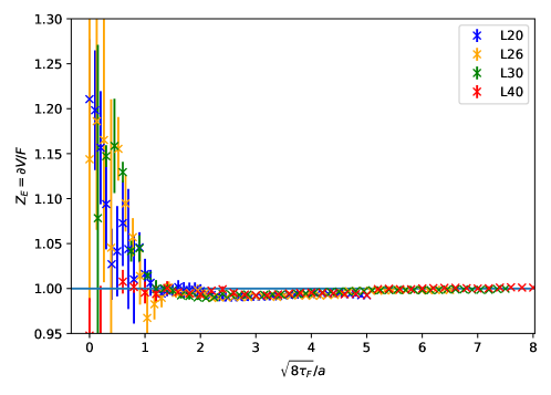
Figure 1: $Z_{E}$ for all lattice sizes with increasing flow time. We see that for flow radii larger than one lattice spacing, the factor $Z_{E}$ becomes practically one.

IV.3 Continuum extrapolation

IV.3.1 Continuum interpolation

Preparing for the continuum limit, we interpolate $r^{2}F$ on all ensembles at a fixed flow time to a common $r$-range in $\sqrt{t_{0}}$-units. We use polynomial interpolations at different orders:

$$P_{n}(r)=\sum_{k=0}^{n}a_{k,n}r^{k}\,,$$ (38)

with $a_{k,n}$ being the coefficients. We have different coefficients for different fixed order polynomials. An interpolation at fixed order corresponds to a single fit, where we minimize the $\chi^{2}$.

In addition, interpolations have the advantage that small fluctuations within the data get smoothed. Polynomial interpolations can have fluctuations, especially higher order polynomial fits, and hence, we average over different polynomial orders to reduce those fluctuations:

$$P_{\mathrm{inter}}(r) =\sum_{n=n_{\mathrm{min}}}^{n_{\mathrm{max}}}w_{n}P_{n}(r)\,,$$ (39)

$$\sum_{n=n_{\mathrm{min}}}^{n_{\mathrm{max}}}w_{n} =1\,,$$ (40)

where $w_{n}$ are normalized, adjustable weights.

For the L20, L26, and L30 lattices, we use equal weights for all polynomial orders. We choose polynomials of orders $n=4,5,6,7$ for L20, orders $n=7,8,9,10$ for L26, and orders $n=8,9,10,11$ for L30. For L40, we use an Akaike average Jay and Neil (2021) over the orders from 4 to 12 because at some flow times the plateau extraction at larger $r$ gives fluctuating results. This results from underestimated systematic effects and causes a change in the effective polynomial orders, which is considered through the Akaike average. The weights are found analogously to Eqs. (30) and (31) through

$$\mathrm{AIC}_{n} =\chi^{2}_{n}+2\,dof\,,$$ (41)

$$w_{n} \propto e^{-\frac{1}{2}\mathrm{AIC}_{n}}\,,$$ (42)

where the final values of $w_{n}$ are fixed by the normalization condition. To propagate the statistical error, the continuum interpolation is done for every jackknife block.

This procedure works for most of the data. An exception is the data at small $r$ (up to $r/a=3$) for the L26 lattice. We obtain a miscarried interpolation in this case due to large $r$ effects in the interpolation. For the L26 lattice, it turns out that spline interpolations up to $r/a=3$ and changing to the polynomial interpolation for larger $r$ works properly.

IV.3.2 Tree level improvement

To reduce the effects of finite lattice spacings, we apply a tree level improvement procedure to the data at finite flow time by dividing out the leading lattice perturbation theory result. Following Fodor et al. (2014), the static energy in lattice perturbation theory at finite flow time can be written as:

$$V_{\mathrm{lat}}(r,\tau_{F})=-C_{F}g^{2}\int\frac{\mathrm{d}^{3}\mathbf{k}}{(2\pi)^{3}}e^{i\mathbf{k}\cdot\mathbf{r}}e^{-2\tau_{F}D^{-1}_{\mathrm{GF}}}D_{\mathrm{MC}}\,,$$ (43)

where we have assumed $a=1$ for simplicity and $D$ is the lattice propagator:

$$D^{-1}=4\sum_{i=1}^{4}\left(\sin^{2}\frac{k_{i}}{2}+c_{w}\sin^{4}\frac{k_{i}}{2}\right)\,;$$ (44)

$c_{w}=0$ for the Wilson action, which we use for the simulation part, $D_{\mathrm{MC}}$, and $c_{w}=1/3$ for the Symanzik action, which we use in the gradient flow equations, $D_{\mathrm{GF}}$. Similarly to the zero flow time case that was derived in Brambilla et al. (2022a), the static force coming from the chromoelectric field insertion reduces to a symmetric finite difference:

$$F_{\mathrm{lat}}(r,\tau_{F})=\frac{V_{\mathrm{lat}}(r+a,\tau_{F})-V_{\mathrm{lat}}(r-a,\tau_{F})}{2a}\,.$$ (45)

Now, we can tree level improve the measured force $F_{\mathrm{meas}}$ by dividing out the leading lattice expression and multiplying by the continuum 1-loop gradient flow expression

$$F_{\mathrm{improved}}(r,\tau_{F})=\frac{\mathcal{F}_{0}(r,\tau_{F})}{F_{\mathrm{lat}}(r,\tau_{F})}F_{\mathrm{meas}}(r,\tau_{F})\,,$$ (46)

where $\mathcal{F}_{0}$ is given by Eq. (16).

IV.3.3 Continuum extrapolation

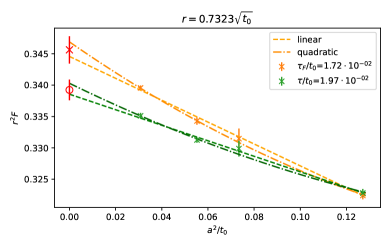
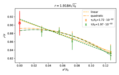
Figure 2: Examples of continuum extrapolation for two different separations $r$. The figure shows the linear and quadratic continuum limits: the line corresponds to the linear limit, the curve to the quadratic one.

We use the interpolated and tree level improved data for the continuum limit, which is obtained from extrapolations linear and quadratic in $a^{2}/t_{0}$ at fixed physical distances $r$ and fixed physical flow times $\tau_{F}$:

$$f^{\mathrm{linear}}(a^{2}/t_{0}) =m\frac{a^{2}}{t_{0}}+c_{l}\,,$$ (47)

$$f^{\mathrm{quadratic}}(a^{2}) =A\frac{a^{4}}{t_{0}^{2}}+B\frac{a^{2}}{t_{0}}+C_{l}\,,$$ (48)

where $m,c_{l},A,B$, and $C_{l}$ are the fit parameters, and $c_{l}$ and $C_{l}$ are the continuum limits of the linear and quadratic extrapolation, respectively. We take an Akaike average, defined for polynomials as in Eqs. (41) and (42). Figure 2 shows a working example for the continuum limit at two fixed distances $r$ and for each distance at two different flow times.

Although we use tree level improved data and Akaike average over linear and quadratic continuum limits, often both $\chi^{2}/dof$ are too large. Hence, we restrict to data which accomplish that at least one of the extrapolations gives $\chi^{2}/dof<3.0$ and that the flow radius fulfills $\sqrt{8\tau_{F}}>a$. The remaining, filtered data represents reliable continuum limit results, with which we continue the further analyses.

IV.4 $r_{0}$ and $r_{1}$ scales

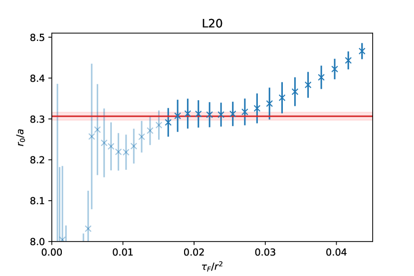
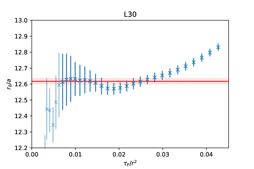
Figure 3: The $r_{0}$ scale along the flow time axis.

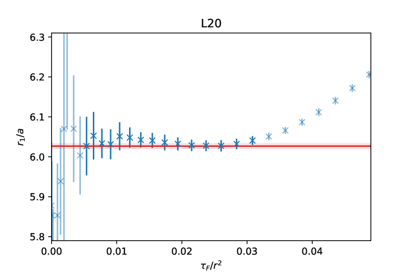
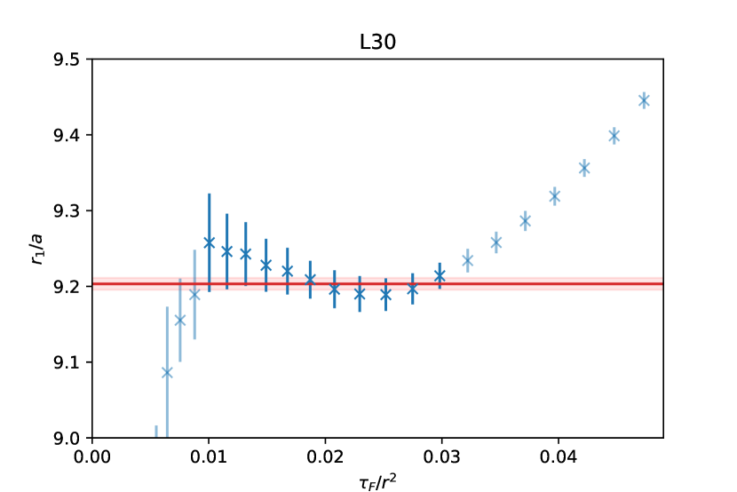
Figure 4: The $r_{1}$ scale along the flow time axis.

	$r_{0}/a$	$\sigma_{\mathrm{stat}}$	$\sigma_{\mathrm{AIC}}$	$\sigma_{\mathrm{stat+AIC}}$	$r_{1}/a$	$\sigma_{\mathrm{stat}}$	$\sigma_{\mathrm{AIC}}$	$\sigma_{\mathrm{stat+AIC}}$
L20	8.306	0.017	0.010	0.020	6.026	0.0090	0.006	0.011
L26	10.833	0.031	0.025	0.040	7.849	0.014	0.010	0.018
L30	12.617	0.032	0.018	0.040	9.203	0.0130	0.008	0.015
L40	16.933	0.042	0.015	0.044	12.316	0.0280	0.011	0.030

Table 3: Results for $r_{0}$ and $r_{1}$ in the zero flow time limit at finite lattice spacing. The table includes the statistical error (stat subscript), the systematic error by choosing different fit ranges (AIC subscript), and the errors added in quadrature.

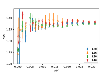
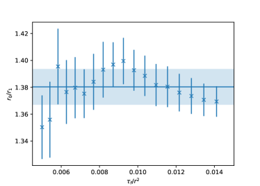
Figure 5: The ratio of the scales $r_{0}$ and $r_{1}$. The left side shows the ratio at finite lattice spacing, the right side the continuum limit with the constant zero flow time extraction.

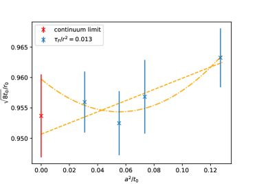
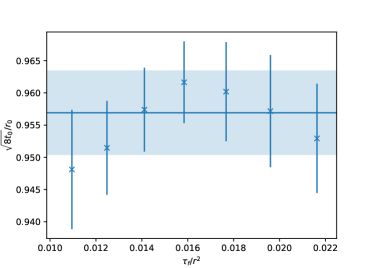
Figure 6: Left: An example for the continuum limit of the ratio $\sqrt{8t_{0}}/r_{0}$ at a fixed flow time ratio. The straight line corresponds to a continuum limit linear in $a^{2}/t_{0}$, the curved line to a polynomial up to quadratic order in $a^{2}/t_{0}$. The red cross and bar is the final continuum limit of a weighted average of both extrapolations. Right: The flowed continuum ratio with the constant zero flow time limit.

In terms of the force $F(r)$, we define a reference scale as

$$r^{2}F(r,\tau_{F})|_{r(c,\tau_{F})}=c\,,$$ (49)

with a dimensionless number $c$. Common choices are $r_{0}(\tau_{F})\equiv r(c=1.65,\tau_{F})$, $r_{0}\equiv r_{0}(\tau_{F}=0)$ Sommer (1994), and $r_{1}(\tau_{F})\equiv r(c=1,\tau_{F})$, $r_{1}\equiv r_{1}(\tau_{F}=0)$ Bernard et al. (2000). In the original proposals, the scales $r(c)$ are defined with the force at zero flow time, however, in our case, the force is computed at different flow times. Thus, we obtain flow time dependent $r_{0}$ and $r_{1}$ as shown in Figs. 3 and 4. To find $r_{0}$ and $r_{1}$, we perform multiple polynomial interpolations of $r^{2}F(r,\tau_{F})$ for larger $r$ along the $r$-axis and at fixed flow time ratio $\tau_{F}/r^{2}$, and find the roots of the individual interpolations as $(r^{2}F)^{\mathrm{inter}}-c=0$. The final scales are given in terms of an Akaike average over the roots of the polynomial interpolators.

Both scales, $r_{0}$ and $r_{1}$, approach a constant plateau within a recognizable flow time regime and start deviating from this plateau at larger flow times. We perform plateau fits within this range for a zero flow time extraction of both scales, and we find them comparable to the scales fixed by Necco and Sommer (2002). The results are shown in table 3. We see that the error of the scale setting is dominated by the statistical fluctuation rather than by the Akaike error of the polynomial interpolators.

The ratio of both scales, $r_{0}(\tau_{F})/r_{1}(\tau_{F})$, is shown in Fig. 5. We take the $a^{2}/t_{0}$ continuum limit followed by a constant zero flow time limit. Finally, we obtain

$$\frac{r_{0}}{r_{1}}=$1.380(14)$.$$ (50)

To our knowledge, there are no prior direct determinations of the scale ratio $r_{0}/r_{1}$ in pure gauge. However, in Ref. Sommer (2014) this ratio was roughly estimated to be $\sim 1.37$ based on the curves shown in Necco and Sommer (2002), which agrees well with our extraction within errors. The extracted value is about 9% larger than the ratio in unquenched theories with 2+1 or 2+1+1 fermion flavors Aoki et al. (2022); Brambilla et al. (2023). Such a shift is to be expected, due to the effect of unquenching of the quark flavors. A similar effect between quenched and unquenched scales has been seen for the gradient flow scale ratios in Ref. Bruno and Sommer (2014).

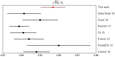
Figure 7: Our extracted ratio (red circle) of the scale ratio $\sqrt{8t_{0}}/r_{0}$ compared to the existing results (black squares) in the literature.

We repeat the same procedure for the ratios $\sqrt{8t_{0}}/r_{0}$ and $\sqrt{8t_{0}}/r_{1}$. Fig. 6 shows an example for the ratio $\sqrt{8t_{0}}/r_{0}$. The final results for the ratios of the scales are

$$\frac{\sqrt{8t_{0}}}{r_{0}} =$0.9569(66)$\,,$$ (51)

$$\frac{\sqrt{8t_{0}}}{r_{1}} =$1.325(13)$\,.$$ (52)

Our extracted ratio $\sqrt{8t_{0}}/r_{0}$ agrees within errors with the previous determinations Lüscher (2010b); Asakawa et al. (2015); Francis et al. (2015); Cè et al. (2015); Kamata and Sasaki (2017); Knechtli et al. (2017); Giusti and Lüscher (2019); Dalla Brida and Ramos (2019), albeit the mean value is slightly above most of the existing results. We show the comparison to the existing literature in Fig. 7. The previous results are somewhat correlated, since most of them focus on $t_{0}$ calculation and use the data from Refs. Guagnelli et al. (1998); Necco and Sommer (2002) at least for part of their dataset for $r_{0}$. Again, the quenched ratios are larger than the unquenched ones Aoki et al. (2022) as has been previously seen in Ref. Bruno and Sommer (2014). To our knowledge, this is the first direct measurement of the scale ratio $\sqrt{8t_{0}}/r_{1}$ in pure gauge.

V Analyses of the continuum results

After having worked out the continuum limit in Sec. IV.3, we compare the lattice results with the perturbative expressions to extract $\Lambda_{0}$. Since gradient flow introduces another scale next to $1/r$, we have several possibilities to compare the lattice results with the perturbative expressions. In the first approach, we use the simple expression of the flowed force in Eq. (22), which turns out to be also applicable to large $r$ results. In the second approach, we compare the lattice results either by keeping the scale $1/r$ fixed and inspecting the behavior along the flow time, or vice versa by keeping $\tau_{F}$ fixed and inspecting the behavior along the distance $r$. We show plots only for the perturbative 1-loop (F1l) and 3-loop with leading ultrasoft resummation (F3lLus) expressions, however, in the result tables we also provide extractions based on the 2-loop with and without leading ultrasoft resummation (F2l and F2lLus), and 3-loop without ultrasoft resummation (F3l) expressions.

V.1 Constant zero flow time limit at fixed $r$

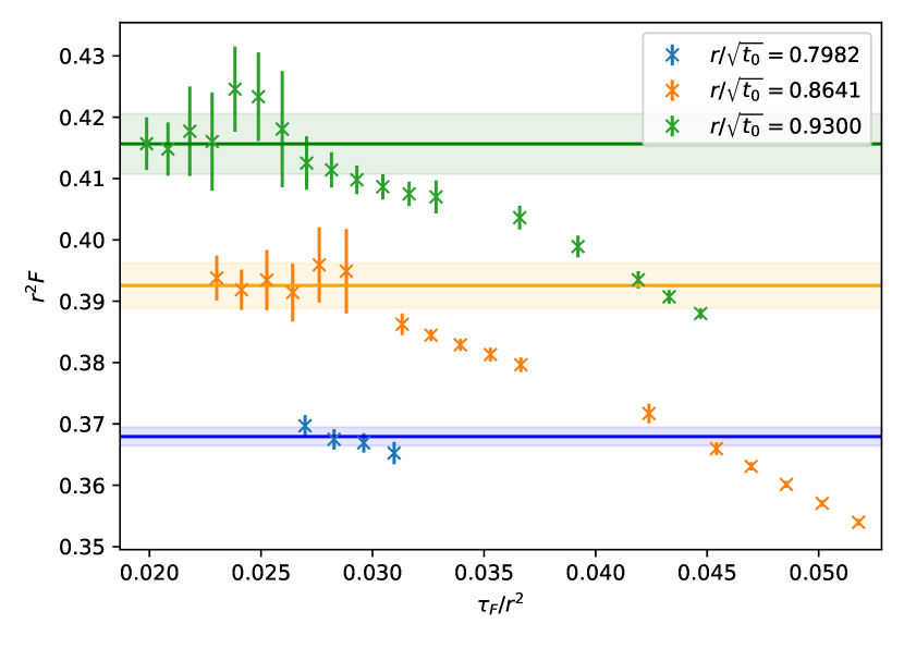
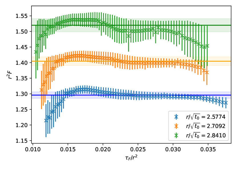
Figure 8: Examples of the flowed force in a regime where a constant behavior can be obtained. The left side shows the data for the smallest $r$ where a constant regime can be obtained. The right side shows the flowed force at larger $r$ where we can apply a constant fit in a proper range of $\tau_{F}/r^{2}$.

We know from Eq. (22) that the static force has a constant behavior at small flow times. Physical quantities are defined at zero flow time; hence, we need to perform the zero flow time limit, $\tau_{F}\rightarrow 0$, while we keep $r$ fixed. In the constant regime, we perform this by a constant fit at fixed distance $r$. Figure 8 shows data where we obtain a constant behavior of the flowed force. The left side shows the data for the smallest $r$ before the smaller flow time comes into conflict with the $\sqrt{8\tau_{F}}>a$ condition. The right side shows data at larger $r$ where the condition $\sqrt{8\tau_{F}}>a$ is fulfilled at even minimal flow time ratios. The small flow time expansion is performed in the ratio $\tau_{F}/r^{2}$, thus, small flow time is defined in the sense of small flow time ratio, which is a dimensionless quantity. The condition $\sqrt{8\tau_{F}}>a$ is given in terms of flow times in physical units; hence, considering this condition in terms of ratio moves it to smaller flow time ratios for larger $r$, since the $r$ in the denominator decreases the ratio.

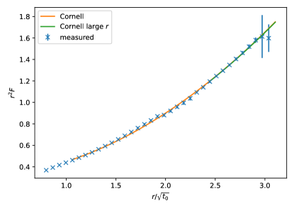
Figure 9: The extracted force from the constant zero flow time limits with two Cornell fits. In a window from $r/\sqrt{t_{0}}\approx 2.1$ to $r/\sqrt{t_{0}}\approx 2.3$, the continuum limit turns out to be difficult to reach. We lose the signal at larger $r$ around $r/\sqrt{t_{0}}\approx 3.0$.

In Fig. 9, we see the final result of the constant zero flow time limits. We identify an increasing behavior with small errors up to $r/\sqrt{t_{0}}\approx 3.0$. Around the distance of $r/\sqrt{t_{0}}\approx 2.25$, we are faced with difficulties to extrapolate to the continuum, and obtain $\chi^{2}/dof$ of order 4 and larger.

We perform a Cornell-fit to the data from $r/\sqrt{t_{0}}\approx 1.1$ to $r/\sqrt{t_{0}}\approx 3.0$ and we obtain

$$r^{2}F(r) =A+\sigma\ r^{2},$$ (53)

$$A =$0.297(6)$\,,$$ (54)

$$\sigma t_{0} =0.151(3).$$ (55)

The string tension $\sigma$ is a quantity that is dominated by the large $r$ regime; hence, in addition, we perform the fit only for data beyond the region where the continuum limits are problematic up to $r/\sqrt{t_{0}}\approx 3.0$. In this case, we obtain

$$A =$0.268(33)$\,,$$ (56)

$$\sigma t_{0} =0.154(6).$$ (57)

The uncertainty for $A$ is five times larger now, which is to be expected, since it is a small $r$ quantity. The results for $\sigma$ from both ranges agree within their uncertainties. With the result in Eq. (51), we can express the string tension in $r_{0}$ units:

$$\sigma r_{0}^{2}=1.345(54).$$ (58)

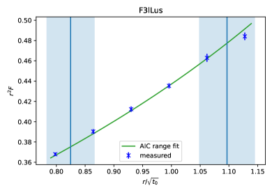
Figure 10: The $\sqrt{8t_{0}}\Lambda_{0}$ extraction with constant zero flow times extrapolation at smallest possible distances $r$. The vertical lines with the dimmer bar represent the lower and upper averaged fit range according to Eqs. (35) and (36).

In the past, the string tension was found to be $\sigma r_{0}^{2}=1.353(3)$ Koma et al. (2007) at finite lattice spacing with $\beta=6.0$, which is in good agreement with our result. Continuum results were obtained in Gonzalez-Arroyo and Okawa (2013); Okawa and Gonzalez-Arroyo (2014) in another reference scale $\bar{r}$. With the ratio $\sqrt{8t_{0}}/\bar{r}$ from Okawa and Gonzalez-Arroyo (2014), these results become $\sigma t_{0}=0.133(2)$ and $\sigma t_{0}=0.143(2)$ respectively. Nevertheless, the ratio $\sqrt{8t_{0}}/\bar{r}$ in Okawa and Gonzalez-Arroyo (2014) is only an approximation over several lattices sizes, and is not extrapolated to the continuum limit. Reliable continuum results for the string tension can be found in  Lucini et al. (2004); Beinlich et al. (1999) in units of the critical temperature $T_{c}$. With the conversion factor $T_{c}\sqrt{t_{0}}$ from Francis et al. (2015), these results become $\sigma t_{0}=0.1484(22)$ and $\sigma t_{0}=0.156(3)$, which agree well with our result.

Order	$\sqrt{8t_{0}}\Lambda_{0}$	$\sigma_{\mathrm{stat}}$	$\sigma_{\mathrm{AIC}}$	$\sigma_{\mathrm{stat+AIC}}$
F1l	0.8214	0.0044	0.0018	0.0047
F2l	0.6635	0.0048	0.0029	0.0056
F2lLus	0.6961	0.0057	0.0039	0.0069
F3l	0.6197	0.0036	0.0024	0.0043
F3lLus	0.6353	0.0032	0.0013	0.0035

Table 4: The fit result for $\sqrt{t_{0}}\Lambda_{0}$ from the constant zero flow time limit extracted data at different orders. We see that the error is dominated by statistical fluctuations rather than the choice of the proper fit window.

At small $r$, we extract $\Lambda_{0}$ from the data by fitting the perturbative force at the available orders. Figure 10 shows examples of the fit for two different orders. Table 4 shows the fit results. We observe that the error is dominated by the statistical fluctuations rather than by the systematic uncertainty due to the choice of the fit ranges.

V.2 Flow time behavior of the force at fixed $r$ or fixed $\tau_{F}$

In the very small $r$ regime, the requirement $\sqrt{8\tau_{F}}>a$ moves the data points along the $\tau_{F}/r^{2}$ axis outside the regime where they are flow time independent even for the smallest possible flow time. Therefore, we compare the lattice data with the full expression of the force, Eq. (23), i.e. without expanding for small $\tau_{F}$.

We inspect the small $r$ flow time behavior, first, at fixed distances $r$, which corresponds to the classical zero flow time limit. In a second approach, we fit along the $r$ axis at fixed flow times to extract $\sqrt{8t_{0}}\Lambda_{0}$. Since the dependence on $\tau_{F}$ of the numerical extraction turns out to be negligible within the distance and flow time regions used for the fits to the lattice data, getting $\sqrt{8t_{0}}\Lambda_{0}$ provides in practice its zero flow time limit.

V.2.1 Fixed $r$

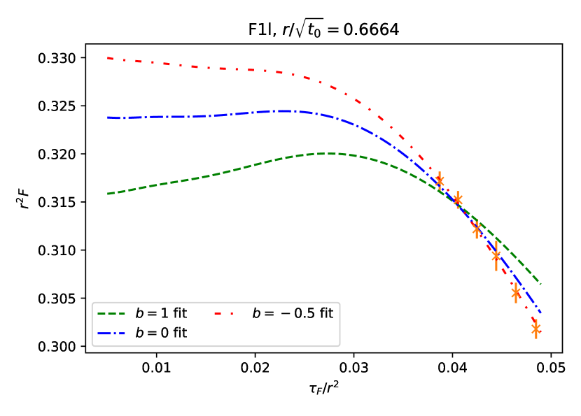
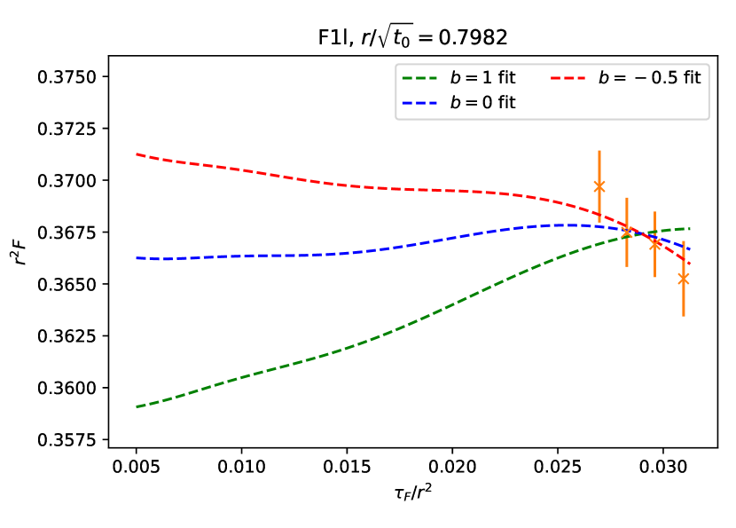
Figure 11: Comparison of different zero flow time limits at 1-loop order at fixed $r$. We compare fits with different scale choices obtained by varying $b$ according to Eq. (21).

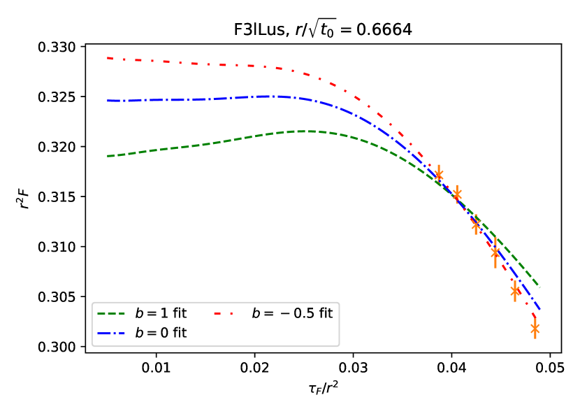
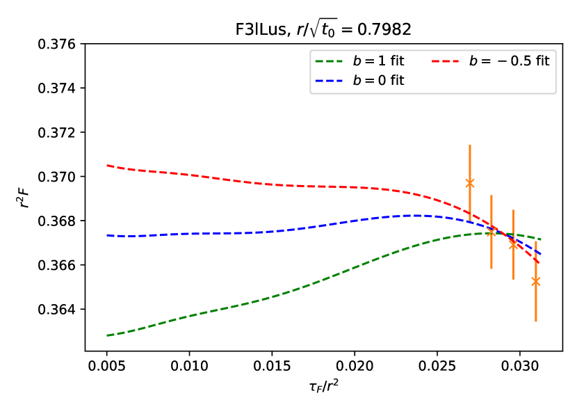
Figure 12: As in Fig. 11, but with the fit function being now the force at 3 loops with leading ultrasoft resummation.

Order	$r/\sqrt{t_{0}}$	$b$	$\sqrt{8t_{0}}\Lambda_{0}$	$\sigma_{\mathrm{stat}}$	$\sigma_{\mathrm{AIC}}$	$\chi^{2}/dof$	$\overline{\tau_{F}/r^{2}}_{\mathrm{Max}}$
F3lLus	0.6664	1	0.6020	0.0030	0.0010	0.57	0.0449(9)
		0	0.6229	0.0031	0.0010	0.52	0.0463(16)
		-0.5	0.6388	0.0029	0.0005	0.22	0.0473(14)
	0.7323	1	0.6128	0.0037	0.0011	0.93	0.0381(14)
		0	0.6300	0.0037	0.0009	0.37	0.0395(20)
		-0.5	0.6427	0.0037	0.0004	0.21	0.0403(19)
	0.7982	1	0.6210	0.0036		0.72
		0	0.6348	0.0037		0.39
		-0.5	0.6440	0.0038		0.23
F2l	0.6664	1	0.6132	0.0032	0.0010	0.59	0.0449(9)
		0	0.6361	0.0033	0.0011	0.51	0.0463(16)
		-0.5	0.6538	0.0031	0.0005	0.20	0.0474(14)
	0.7323	1	0.6274	0.0040	0.0012	0.97	0.0381(13)
		0	0.6468	0.0041	0.0010	0.38	0.0395(20)
		-0.5	0.6612	0.0040	0.0005	0.20	0.0404(19)
	0.7982	1	0.6394	0.0040		0.77
		0	0.6555	0.0041		0.41
		-0.5	0.6663	0.0042		0.23
F1l	0.6664	1	0.7550	0.0036	0.0010	0.86	0.0446(6)
		0	0.7952	0.0038	0.0012	0.43	0.0466(16)
		-0.5	0.8276	0.0037	0.0001	0.04	0.0476(13)
	0.7323	1	0.7696	0.0045	0.0013	1.33	0.0376(9)
		0	0.8042	0.0048	0.0013	0.49	0.0393(20)
		-0.5	0.8304	0.0048	0.0003	0.12	0.0405(19)
	0.7982	1	0.7829	0.0045		1.29
		0	0.8125	0.0048		0.59
		-0.5	0.8328	0.0050		0.26

Table 5: Fit results at fixed $r$ along the flow time axis for three different choices of the perturbative order of the static force. We start at the smallest possible flow time and use an Akaike range fit for different upper limits. No value for $\sigma_{\mathrm{AIC}}$ indicates that there are not enough points along the flow time to perform an Akaike range fit. The given $\chi^{2}/dof$ corresponds to the most likely fit range. $\overline{\tau_{F}/r^{2}}_{\mathrm{Max}}$ gives the Akaike averaged upper flow time limit.

Figures 11 and 12 show the flow time behavior of the force at two different fixed $r$ along the flow time axis. We compare our lattice data with the perturbative expressions of the force at different orders and fit them to the data. $\Lambda_{0}$ serves as the fit parameter. In the figures, we show the fit results for the case of different, but fixed choices of $b$ in Eq. (21). The fit range starts at the smallest possible flow time. For the upper bound, we take an Akaike average Jay and Neil (2021) over different fit ranges to reduce the systematics due to the fit range choice.

From the figures, we get that the choice of the scale parameter $b$ has a definitive effect on how well the perturbative curve describes the data. A value of $b=1$ guarantees the correct asymptotic behavior at large flow time Brambilla et al. (2022b). However, we see that $b=1$ is the worst of our $b$ choices at describing the actual lattice data in the range of flow times we are interested in. Hence, we use negative values of $b$, which still lead to valid scaling in our range of flow times, as discussed in Appendix A. At small $r$ (left side plots in Figs. 11 and 12), the slope along the flow time is strong, while at the largest $r$ to which we can reasonably apply fixed $r$ fits (right side plots in Figs. 11 and 12), the data points seem already sensitive to the constant behavior of the force expected at small flow times. At small flow times within our considered flow time range, the fits with $b=0$ and $b=-0.5$ agree reasonably well with the data. Table 5 shows an incomplete part of the fit results.

We conclude that for smaller $r$, which requires going to larger flow time ratios $\tau_{F}/r^{2}$, a negative value of $b$ describes the data better in the large flow time regime than $b=0$ or 1, whereas for larger $r$ all choices might describe the data within the given uncertainties. That means that fixing $b$ introduces another source of uncertainty which has to be considered. In the zero flow time limit, all choices of $b$ give $\mu=1/r$, which is the natural scale choice for the static force and energy at zero flow time.

V.2.2 Fixed $\tau_{F}$

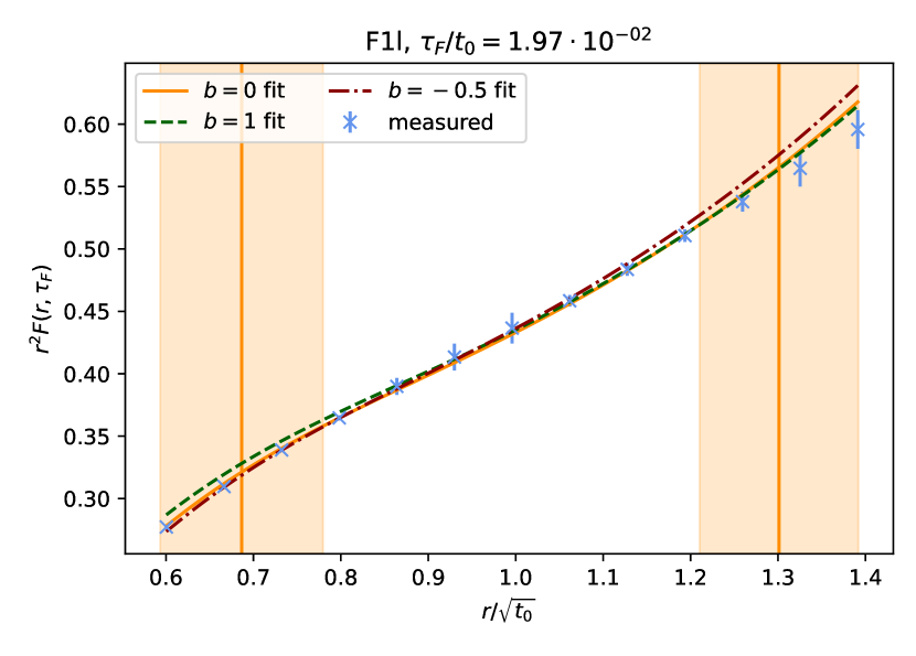
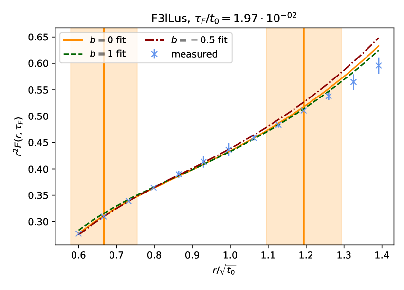
Figure 13: $\sqrt{8t_{0}}\Lambda_{0}$ fit at fixed flow time for different orders. The left vertical line corresponds to the average lower fit limit for $b=0$, and the right line to its average upper fit limit. The bands around the lines represent the errors of the fit window.

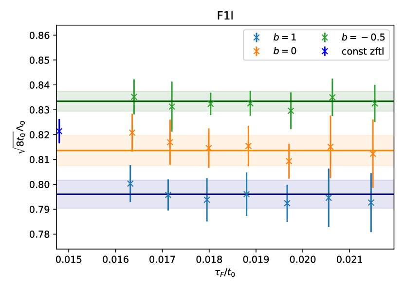
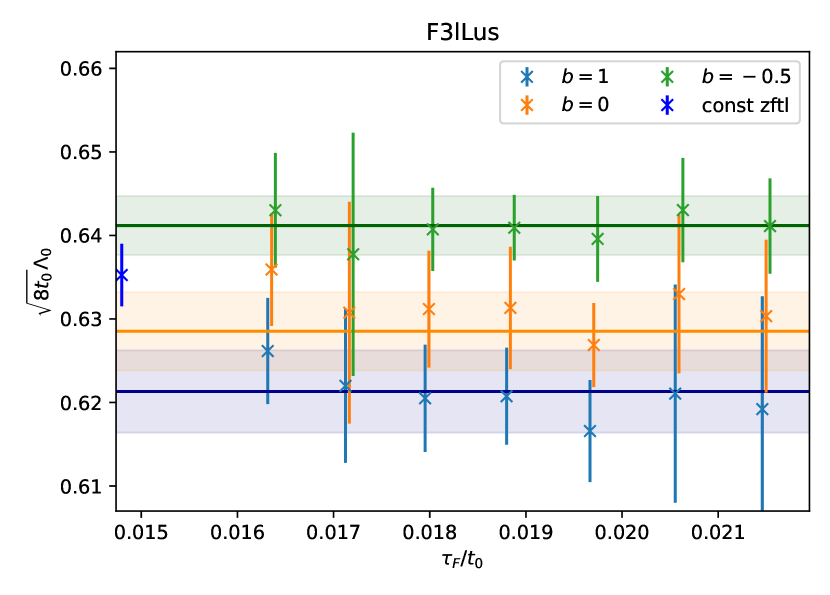
Figure 14: $\sqrt{8t_{0}}\Lambda_{0}$ in the zero flow time limit from a constant fit including the statistical and fit errors. We compare different orders and different choices of $b$. The blue points with the label “const zftl” are the results from table 4.

$b$-scale	F1l	F2l	F2lLus	F3l	F3lLus
1	0.7972(56)	0.6591(49)	0.6911(52)	0.6062(52)	0.6218(50)
0	0.8134(57)	0.6649(47)	0.6982(54)	0.6154(44)	0.6287(44)
-0.5	0.8334(42)	0.6709(47)	0.7017(53)	0.6285(35)	0.6415(36)

Table 6: Results of the $\sqrt{8t_{0}}\Lambda_{0}$ extraction from the constant zero flow time limit of $\Lambda_{0}$ at fixed flow time. The error includes the statistical and the AIC error from the fit.

In the next step, we use data at fixed flow times $\tau_{F}$ and fit the perturbative force along the $r$-axis. We use Akaike average Jay and Neil (2021) over different fit windows for reducing systematics by choosing the right fit window. We perform one-parametric fits at fixed $b$ for $\sqrt{8t_{0}}\Lambda_{0}$. Figure 13 shows an example fit for $b=0,1,-0.5$ for F1l and F3lLus at the same flow time. The left vertical line with the dimmer band corresponds to the average lower fit limit for the $b=0$ fit, and the right vertical line to its average upper limit.

We observe that the $b=0$ fit describes the data over a wide $r$ range from small to larger $r$. The $b=1$ fit describes the data around $r/\sqrt{t_{0}}=1$ and up to larger $r$ in the same way as the $b=0$ fit, but deviates from the data at smaller $r$ in contrast to the $b=0$ fit. This matches with its lower fit range limit being at larger $r$, but the upper fit range limit being the same as in the $b=0$ fit, indicating that the effective fit range for $b=1$ is more on the larger $r$ side. The $b=-0.5$ fit describes the data around $r/\sqrt{t_{0}}=1$ likewise the $b=0$ and $b=1$ fits, but in contrast to the $b=1$ case, it fits better to the data at small $r$ and deviates from the data at larger $r$. This matches with its upper fit range limit being at smaller $r$, but the lower fit range limit being the same as in the $b=0$ fit, indicating that the effective fit range for $b=-0.5$ is more on the smaller $r$ side. We conclude that the range for $b$ from $-0.5$ to $1$ fits well to the data, but with different effective fit ranges. The $b=0$ fit has the widest effective fit range and will serve as our default choice.

Figure 14 shows the fit results for $\sqrt{8t_{0}}\Lambda_{0}$ at the valid flow time positions for $b=1,0,-0.5$ at F1l and F3lLus. We observe that for a fixed choice of $b$, the values of $\Lambda_{0}$ are constant along the flow time axis. This indicates that the flow time dependence of the static force at finite flow time in the distance and flow time ranges explored in this fixed $\tau_{F}$ analysis is well captured by a constant 1-loop gradient flow correction to the static force. We then extrapolate $\Lambda_{0}$ to the zero flow time limit with a constant function. The final results of the constant zero flow time limits are shown in table 6.

V.3 Estimate of the perturbative systematic uncertainties and final results

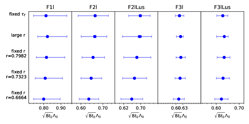
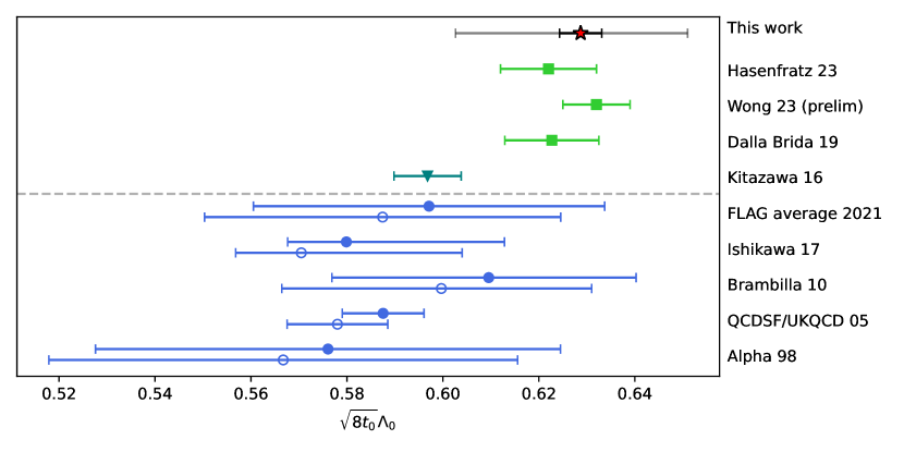
Figure 15: The final results for $\sqrt{8t_{0}}\Lambda_{0}$. Left: Comparison of all fit results for all methods and for all orders. The inner error bar corresponds to the combined statistical and AIC errors, when applicable. The outer error bar represents the total error, including the systematic uncertainties from the scale variation. The row “large $r$” shows the results from the first method, where we perform the constant zero flow time limit of the force first. Right: Our final result compared to the literature. The points above the dashed line were determined with gradient flow based scale settings, $t_{0}$ (squares) or $w_{0}$ (triangle), while the lower points (circles) are converted from $r_{0}$ units with either our ratio Eq. (51) (filled points), or with the ratio from Dalla Brida and Ramos (2019) (hollow points).

Up to this point, we have presented results for $\Lambda_{0}$ with error estimates that include only the statistical errors and the systematic errors from choosing different fit ranges. We still need to include the perturbative uncertainty from the unknown higher-order terms in the perturbative expansion. We can do this by varying the scale $\mu$ (21). In previous studies of the static energy Bazavov et al. (2019, 2014, 2012), the zero flow time scale $\mu=1/r$ was varied by a factor of $\sqrt{2}$. We make here the same choice and vary the parameter $s$ in Eq. (21) from $s=0.5$ to $s=2$. We vary the $s$-parameter only in the zero flow time part of Eq. (23) and keep it fixed at $s=1$ in the finite flow time part. In principle, we could vary the scale by a factor of $2$ instead of $\sqrt{2}$, but it was noted in Ref. Bazavov et al. (2019) that this requires access to quite small distances $r$. Our current data does not contain small enough distances to allow for this wider variation.

As already stated in the previous sections, the finite flow time part of the static force has a considerable dependence on the choice of the parameter $b$ in Eq. (21). To match the conventions of zero flow time studies, we choose $b=0$ as our main result. To estimate the systematic error due to the choice of $b$ and the missing higher order finite flow time perturbative terms, we vary the $b$ parameter between $b=-0.5$ and $b=1$; for this choice, we refer to the discussion in appendix A. We vary $b$ only in the finite flow time part of the Eq. (23).

To arrive at a final result for $\Lambda_{0}$, we have explored several possibilities in sections V.1, V.2.1, and V.2.2:

1. We have performed the constant zero flow time limit of the force first, followed by fitting the perturbative expression to the data. This method has the advantage that we do not need to combine the zero flow time expression of the force with the 1-loop correction coming from the gradient flow. The method does not work, however, at the smallest $r$, but only for $r/\sqrt{t_{0}}\geq 0.8$.

2. We have performed the fit of the combined equation at fixed $r$ along $\tau_{F}$. This method corresponds to the classical zero flow time limit. With this method, the $1/r$ scale has a minor effect and the method can be applied for only few $r$, while the gradient flow scale has a dominant role, which can be seen by the large dependence on the choice of $b$.

3. We have performed the fit of the combined equation at fixed $\tau_{F}$ along $r$. In this method, the $1/r$ scale has a major impact, while the flow time scale has a minor role. This can be seen by the fact that various choices of $b$ fit well to the data.

On the left side of Fig. 15, we compare the results of all three methods at the available perturbative orders. All results agree very well within the errors.

Based on the advantages and disadvantages of all three methods, we chose method 3 with $b=0$ at F3lLus as the main result. Including the uncertainties due to variations of the parameters $s$ and $b$, we obtain our final result, which reads

$$\sqrt{8t_{0}}\Lambda_{0} =0.629^{+22}_{-26}\,,$$ (59)

$$\delta(\sqrt{8t_{0}}\Lambda_{0}) =(4)^{\mathrm{lattice}}(^{+18}_{-25})^{\mathrm{s-scale}}(^{+13}_{-7})^{\mathrm{b-scale}},$$ (60)

where $(...)^{\mathrm{lattice}}$ stands for the error coming from the statistics and choosing different fit windows. As we allow the parameters $b$ and $s$ in Eq. (21) to be varied only in the finite and zero flow time part respectively, it follows that the systematic uncertainties from these variations are nearly independent one from the other. Hereby, we quote the uncertainty from the $b$ scale variation measured at $s=1$ and the uncertainty from the $s$ scale variation measured at $b=0$, and add these in quadrature. This accounts for a conservative estimate of the perturbative error.

On the right side of Fig. 15, we compare our final result with results from previous measurements of $\Lambda_{0}$ Capitani et al. (1999); Gockeler et al. (2006); Brambilla et al. (2010); Ishikawa et al. (2017); Kitazawa et al. (2016); Dalla Brida and Ramos (2019); Wong et al. (2023); Hasenfratz et al. (2023) and the FLAG average Aoki et al. (2022). We only show previous studies that contribute to the FLAG average and a couple of newer studies that have come out since the latest FLAG average. In Fig. 15, the points above the dashed line have been obtained using the gradient flow based scales $t_{0}$ and $w_{0}$, while the points below the dashed line have been obtained from the scale $r_{0}$. For the measurements done in the $r_{0}$ scale, we convert to the $t_{0}$ scale with our own ratio (51) (filled points) or with one of the ratios from Ref. Dalla Brida and Ramos (2019) (empty points). We find it remarkable that all the newer studies done in $t_{0}$ units are on the higher end of the measurements. Furthermore, we note that our error is larger than other recent studies. Our error is dominated by the perturbative error from the scale variation. Since the scale variation is more prominent at larger distances, it is to be expected that future access to finer lattices could bring this error down. Lastly, with the ratio in Eq. (51), we can convert our final result into $r_{0}$ units and obtain

$$r_{0}\Lambda_{0}=0.657^{+23}_{-28}\,.$$ (61)

VI Summary and conclusion

We have shown that the gradient flow renormalizes an operator made of a Wilson loop with a chromoelectric field insertion by reducing discretization effects and in this way improving the convergence towards the continuum limit. This result can be of use for further studies on operators with different field insertions, which typically show up in nonrelativistic effective field theories.

Thanks to the above property, we are able to perform the continuum limit of the static force at finite flow time, and extrapolate to zero flow time in three different ways. In the first method, we extrapolate the static force from a constant zero flow time limit. This works for large and intermediate $r$, but not at very short distances in the regime $r/\sqrt{t_{0}}<0.8$. At large distances, we extract the scales $r_{0}$ and $r_{1}$, and are able to perform a Cornell fit. For the scales, we find the ratios

$$\frac{r_{0}}{r_{1}} =$1.380(14)$\,,$$ (62)

$$\frac{\sqrt{8t_{0}}}{r_{0}} =$0.9569(66)$\,,$$ (63)

$$\frac{\sqrt{8t_{0}}}{r_{1}} =$1.325(13)$\,,$$ (64)

and for the string tension parameter in the Cornell fit, we find

$$\sigma t_{0} =0.154(6)\,,$$ (65)

$$\sigma r_{0}^{2} =1.345(54)\,,$$ (66)

where we have used our result for the ratio $\sqrt{8t_{0}}/r_{0}$ in Eq. (63) to convert into $r_{0}$ units. At short distances, we fit the perturbative force to the data, and obtain at F3lLus order

$$\sqrt{8t_{0}}\Lambda_{0}=$0.635(4)$\,.$$ (67)

In the second and third method, we fit with a function that combines the force at zero flow time up to 3 loops with the 1-loop flow time correction. In this way, the fit function depends on two scales, $r$ and $\tau_{F}$. In the second method, we keep $r$ fixed and perform the fit along $\tau_{F}$. In the third method, we keep $\tau_{F}$ fixed and perform the fit along $r$, and extrapolate the resulting $\Lambda_{0}(\tau_{F})$ to the zero flow time limit. The third method has, in comparison to the second method, a strong dependence on the scale $1/r$, which is the dominant physical scale. Furthermore, the third method reaches out to small $r$ in contrast to the first method. Therefore, we take the third method as our reference method and obtain

$$\sqrt{8t_{0}}\Lambda_{0} =0.629_{-26}^{+22}\,,$$ (68)

$$\delta(\sqrt{8t_{0}}\Lambda_{0}) =(4)^{\mathrm{lattice}}(_{-25}^{+18})^{\mathrm{s-scale}}(_{-7}^{+13})^{\mathrm{b-scale}}.$$ (69)

Using the ratio in Eq. (63), we can give our final result in $r_{0}$ units as

$$r_{0}\Lambda_{0}=0.657^{+23}_{-28}\,.$$ (70)

Nevertheless, all methods agree well within their errors, with an overlap of almost $70\text{\,}\mathrm{\char 37\relax}$.

Appendix A About negative values of $b$ in $\mu$

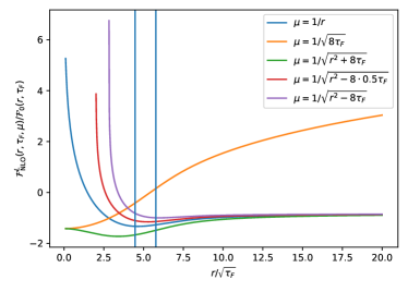
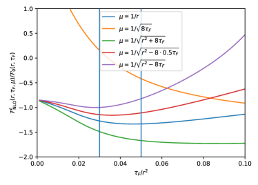
Figure 16: Left: The ratio $\mathcal{F}_{\mathrm{NLO}}^{L}(r,\tau_{F},\mu)/\mathcal{F}_{0}(r,\tau_{F})$ (see Eq. (15)) as a function of $r/\sqrt{\tau_{F}}$ plotted for various values of $s$ and $b$. The vertical lines represent the characteristic flow time window of this study. The left limit on the $x$-axis corresponds to the infinite flow time limit, while the right limit to the zero flow time limit. Right: The same ratio, but as a function of $\tau_{F}/r^{2}$ zoomed around the region of interest.

In the analysis done in section V, we chose the scale (21) with different values for $b$, including negative values. The ratio $\mathcal{F}_{\mathrm{NLO}}^{L}(r,\tau_{F},\mu)/\mathcal{F}_{0}(r,\tau_{F})$ for different values of the parameters $s$ and $b$ is shown in Fig. 16. In Brambilla et al. (2022b), the choices $b=1,0$ with $s=1$, and $b=1$ with $s=0$ were also analyzed. The choice $s=1$, $b=0$ is the natural choice at zero flow time, since for it $\log(\mu r)$ terms vanish. However, this choice does not capture $\log(\mu\sqrt{\tau_{F}})$ terms that become important at large flow time. This is shown by the ratio $\mathcal{F}_{\mathrm{NLO}}^{L}(r,\tau_{F},\mu)/\mathcal{F}_{0}(r,\tau_{F})$ becoming large at large flowtimes for this choice of parameters. The choice $s=0$, $b=1$ is the natural choice at large flow time, since for it $\log(\mu\sqrt{\tau_{F}})$ terms vanish. However, this choice does not capture $\log(\mu r)$ terms that become important at small flow time. This is shown by the ratio $\mathcal{F}_{\mathrm{NLO}}^{L}(r,\tau_{F},\mu)/\mathcal{F}_{0}(r,\tau_{F})$ becoming large at small flow times for this choice of parameters. The choice $s=1$ and $b=1$ interpolates between these two extreme and provides a small $\mathcal{F}_{\mathrm{NLO}}^{L}(r,\tau_{F},\mu)$ correction with respect to the leading gradient flow term $\mathcal{F}_{0}(r,\tau_{F})$ over the whole range of flow times. Also the overall scale dependence turns out to be weak with this scale choice.

Nevertheless, our lattice data explore a very specific and limited region of flow time values, the one in between the vertical lines in Fig. 16. This region is zoomed in in the right plot that makes manifest that different choices of $b$, keeping $s=1$, provide, indeed, even smaller and more stable corrections $\mathcal{F}_{\mathrm{NLO}}^{L}(r,\tau_{F},\mu)$ in the region of interest than the choice $b=1$. In particular, this is the case for $b=0$ and $b=-0.5$, which indeed best fit our lattice data, as we have discussed in the main body of the paper. More negative values of $b$ further reduce the relative size of $\mathcal{F}_{\mathrm{NLO}}^{L}(r,\tau_{F},\mu)$, but make it more scale dependent. Hence, the 1-loop expression of the gradient flow expression of the force suggests that for $0.03\lesssim\tau_{F}/r^{2}\lesssim 0.05$ the ideal choice of the parameter $b$ is in between 0 and a negative number larger than $-1$. This is confirmed by the lattice data. Clearly also a parameterization with negative $b$ must smoothly go over $\mu=1/\sqrt{\tau_{F}}$ at large flow time. However, the specific form of the parametrization at large flow times, $\tau_{F}/r^{2}>0.05$, cannot be explored with the present data.

Appendix B Flow time dependence of the Wilson loops with and without chromoelectric field insertions

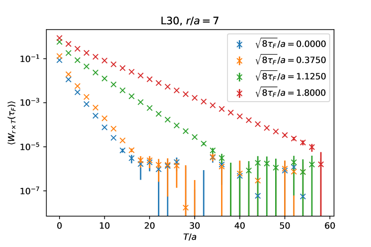
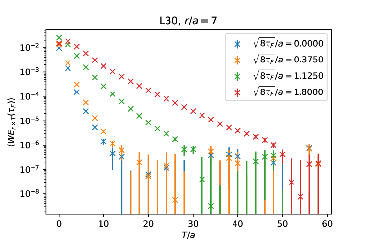
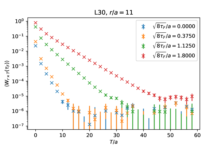
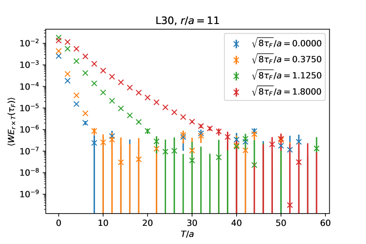
Figure 17: The left sides show the $T$-dependence of the Wilson loops at four different fixed flow times and for two fixed $r$. The right sides show the same for the Wilson loops with a chromoelectric field insertion.

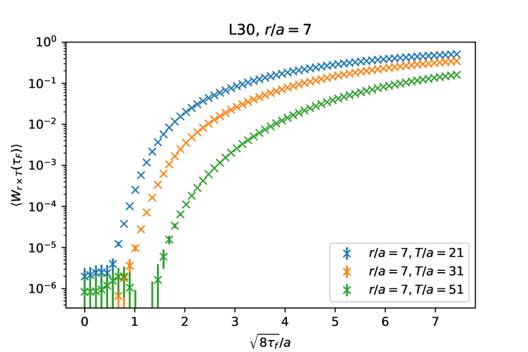
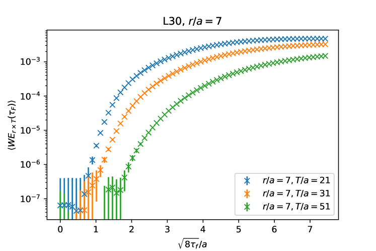
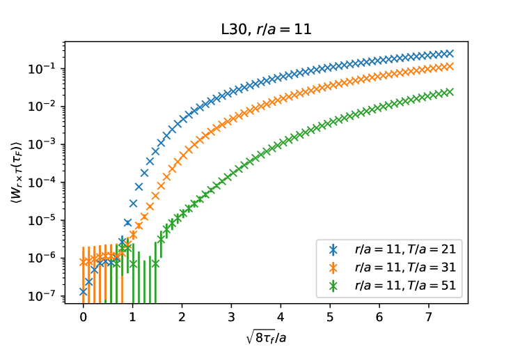
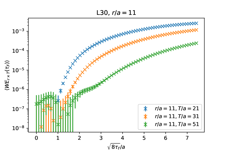
Figure 18: The left sides show the flow time dependence of the Wilson loop at several fixed $T$ and at two different $r$. The right sides show the same for the Wilson loops with a chromoelectric field insertion.

The Wilson loops with and without chromoelectric field insertion are the main objects of this work, therefore, it is worth to have a closer look on the flow time dependence of them. Figure 17 shows the $T$ dependence of the Wilson loops at different flow times. In a logarithmic $y$-scale, we see linear, decreasing curves for large $T$, which correspond to the exponential fall off controlled by the static energy. For zero and small flow times, the slope is the same, for larger flow times the slope becomes more flat. This reflects the flow time dependency of the static energy. This observation holds for Wilson loops with and without chromoelectric field insertions.

Figure 18 shows the flow time dependence of the Wilson loops with and without chromoelectric field insertion at fixed $r$ and $T$. We see a strong flow time dependence for both cases caused by the divergence of the static quark propagator. The strong flow time dependence cancels in the ratio of the Wilson loops.

References

- Aoki et al. (2022) Y. Aoki et al. (Flavour Lattice Averaging Group (FLAG)), “FLAG Review 2021,” Eur. Phys. J. C 82, 869 (2022), arXiv:2111.09849 [hep-lat] .
- d’Enterria et al. (2022) D. d’Enterria et al., “The strong coupling constant: State of the art and the decade ahead,” (2022), arXiv:2203.08271 [hep-ph] .
- Dalla Brida et al. (2022) Mattia Dalla Brida, Roman Höllwieser, Francesco Knechtli, Tomasz Korzec, Alessandro Nada, Alberto Ramos, Stefan Sint, and Rainer Sommer (ALPHA), “Determination of by the non-perturbative decoupling method,” Eur. Phys. J. C 82, 1092 (2022), arXiv:2209.14204 [hep-lat] .
- Necco and Sommer (2002) Silvia Necco and Rainer Sommer, “The N(f) = 0 heavy quark potential from short to intermediate distances,” Nucl. Phys. B 622, 328–346 (2002), arXiv:hep-lat/0108008 .
- Guagnelli et al. (1998) Marco Guagnelli, Rainer Sommer, and Hartmut Wittig (ALPHA), “Precision computation of a low-energy reference scale in quenched lattice QCD,” Nucl. Phys. B 535, 389–402 (1998), arXiv:hep-lat/9806005 .
- Sommer (1994) R. Sommer, “A New way to set the energy scale in lattice gauge theories and its applications to the static force and in SU(2) Yang-Mills theory,” Nucl. Phys. B 411, 839–854 (1994), arXiv:hep-lat/9310022 .
- Bali and Schilling (1993) Gunnar S. Bali and Klaus Schilling, “Running coupling and the Lambda parameter from SU(3) lattice simulations,” Phys. Rev. D 47, 661–672 (1993), arXiv:hep-lat/9208028 .
- Booth et al. (1992) S. P. Booth, D. S. Henty, A. Hulsebos, A. C. Irving, Christopher Michael, and P. W. Stephenson (UKQCD), “The Running coupling from SU(3) lattice gauge theory,” Phys. Lett. B 294, 385–390 (1992), arXiv:hep-lat/9209008 .
- Brambilla et al. (2010) Nora Brambilla, Xavier Garcia i Tormo, Joan Soto, and Antonio Vairo, “Precision determination of from the QCD static energy,” Phys. Rev. Lett. 105, 212001 (2010), [Erratum: Phys.Rev.Lett. 108, 269903 (2012)], arXiv:1006.2066 [hep-ph] .
- Husung et al. (2018) Nikolai Husung, Mateusz Koren, Philipp Krah, and Rainer Sommer, “SU(3) Yang Mills theory at small distances and fine lattices,” EPJ Web Conf. 175, 14024 (2018), arXiv:1711.01860 [hep-lat] .
- Husung et al. (2020) Nikolai Husung, Peter Marquard, and Rainer Sommer, “Asymptotic behavior of cutoff effects in Yang–Mills theory and in Wilson’s lattice QCD,” Eur. Phys. J. C 80, 200 (2020), arXiv:1912.08498 [hep-lat] .
- Jansen et al. (2012) Karl Jansen, Felix Karbstein, Attila Nagy, and Marc Wagner (ETM), “ from the static potential for QCD with dynamical quark flavors,” JHEP 01, 025 (2012), arXiv:1110.6859 [hep-ph] .
- Karbstein et al. (2014) Felix Karbstein, Antje Peters, and Marc Wagner, “ from a momentum space analysis of the quark-antiquark static potential,” JHEP 09, 114 (2014), arXiv:1407.7503 [hep-ph] .
- Bazavov et al. (2012) Alexei Bazavov, Nora Brambilla, Xavier Garcia i Tormo, Peter Petreczky, Joan Soto, and Antonio Vairo, “Determination of from the QCD static energy,” Phys. Rev. D 86, 114031 (2012), arXiv:1205.6155 [hep-ph] .
- Bazavov et al. (2014) Alexei Bazavov, Nora Brambilla, Xavier Garcia Tormo, I, Peter Petreczky, Joan Soto, and Antonio Vairo, “Determination of from the QCD static energy: An update,” Phys. Rev. D 90, 074038 (2014), [Erratum: Phys.Rev.D 101, 119902 (2020)], arXiv:1407.8437 [hep-ph] .
- Takaura et al. (2019) Hiromasa Takaura, Takashi Kaneko, Yuichiro Kiyo, and Yukinari Sumino, “Determination of from static QCD potential: OPE with renormalon subtraction and lattice QCD,” JHEP 04, 155 (2019), arXiv:1808.01643 [hep-ph] .
- Bazavov et al. (2019) Alexei Bazavov, Nora Brambilla, Xavier Garcia i Tormo, Péter Petreczky, Joan Soto, Antonio Vairo, and Johannes Heinrich Weber (TUMQCD), “Determination of the QCD coupling from the static energy and the free energy,” Phys. Rev. D 100, 114511 (2019), arXiv:1907.11747 [hep-lat] .
- Ayala et al. (2020) Cesar Ayala, Xabier Lobregat, and Antonio Pineda, “Determination of from an hyperasymptotic approximation to the energy of a static quark-antiquark pair,” JHEP 09, 016 (2020), arXiv:2005.12301 [hep-ph] .
- Brambilla et al. (1999) Nora Brambilla, Antonio Pineda, Joan Soto, and Antonio Vairo, “The Infrared behavior of the static potential in perturbative QCD,” Phys. Rev. D 60, 091502 (1999), arXiv:hep-ph/9903355 .
- Pineda and Soto (2000) Antonio Pineda and Joan Soto, “The Renormalization group improvement of the QCD static potentials,” Phys. Lett. B 495, 323–328 (2000), arXiv:hep-ph/0007197 .
- Brambilla et al. (2007) Nora Brambilla, Xavier Garcia i Tormo, Joan Soto, and Antonio Vairo, “The Logarithmic contribution to the QCD static energy at N**4 LO,” Phys. Lett. B 647, 185–193 (2007), arXiv:hep-ph/0610143 .
- Brambilla et al. (2009) Nora Brambilla, Antonio Vairo, Xavier Garcia i Tormo, and Joan Soto, “The QCD static energy at NNNLL,” Phys. Rev. D 80, 034016 (2009), arXiv:0906.1390 [hep-ph] .
- Anzai et al. (2010) C. Anzai, Y. Kiyo, and Y. Sumino, “Static QCD potential at three-loop order,” Phys. Rev. Lett. 104, 112003 (2010), arXiv:0911.4335 [hep-ph] .
- Smirnov et al. (2010) Alexander V. Smirnov, Vladimir A. Smirnov, and Matthias Steinhauser, “Three-loop static potential,” Phys. Rev. Lett. 104, 112002 (2010), arXiv:0911.4742 [hep-ph] .
- Vairo (2016a) Antonio Vairo, “A low-energy determination of at three loops,” EPJ Web Conf. 126, 02031 (2016a), arXiv:1512.07571 [hep-ph] .
- Vairo (2016b) Antonio Vairo, “Strong coupling from the QCD static energy,” Mod. Phys. Lett. A 31, 1630039 (2016b).
- Brambilla et al. (2001) Nora Brambilla, Antonio Pineda, Joan Soto, and Antonio Vairo, “The QCD potential at O(1/m),” Phys. Rev. D 63, 014023 (2001), arXiv:hep-ph/0002250 .
- Brambilla et al. (2022a) Nora Brambilla, Viljami Leino, Owe Philipsen, Christian Reisinger, Antonio Vairo, and Marc Wagner, “Lattice gauge theory computation of the static force,” Phys. Rev. D 105, 054514 (2022a), arXiv:2106.01794 [hep-lat] .
- Narayanan and Neuberger (2006) R. Narayanan and H. Neuberger, “Infinite N phase transitions in continuum Wilson loop operators,” JHEP 03, 064 (2006), arXiv:hep-th/0601210 .
- Lüscher (2010a) Martin Lüscher, “Trivializing maps, the Wilson flow and the HMC algorithm,” Commun. Math. Phys. 293, 899–919 (2010a), arXiv:0907.5491 [hep-lat] .
- Lüscher (2010b) Martin Lüscher, “Properties and uses of the Wilson flow in lattice QCD,” JHEP 08, 071 (2010b), [Erratum: JHEP 03, 092 (2014)], arXiv:1006.4518 [hep-lat] .
- Risch et al. (2023) Andreas Risch, Stefan Schaefer, and Rainer Sommer, “The influence of gauge field smearing on discretisation effects,” PoS LATTICE2022, 384 (2023), arXiv:2212.04000 [hep-lat] .
- Risch (2023) Andreas Risch, “Gauge field smearing and controlled continuum extrapolations,” in 40th International Symposium on Lattice Field Theory (2023) arXiv:2310.06587 [hep-lat] .
- Okawa and Gonzalez-Arroyo (2014) Masanori Okawa and Antonio Gonzalez-Arroyo, “String tension from smearing and Wilson flow methods,” PoS LATTICE2014, 327 (2014), arXiv:1410.7862 [hep-lat] .
- Bazavov et al. (2023) Alexei Bazavov, Daniel Hoying, Olaf Kaczmarek, Rasmus N. Larsen, Swagato Mukherjee, Peter Petreczky, Alexander Rothkopf, and Johannes Heinrich Weber, “Un-screened forces in Quark-Gluon Plasma?” (2023), arXiv:2308.16587 [hep-lat] .
- Bazavov and Chuna (2021) Alexei Bazavov and Thomas Chuna, “Efficient integration of gradient flow in lattice gauge theory and properties of low-storage commutator-free Lie group methods,” (2021), arXiv:2101.05320 [hep-lat] .
- Brambilla et al. (2022b) Nora Brambilla, Hee Sok Chung, Antonio Vairo, and Xiang-Peng Wang, “QCD static force in gradient flow,” JHEP 01, 184 (2022b), arXiv:2111.07811 [hep-ph] .
- Leino et al. (2022) Viljami Leino, Nora Brambilla, Julian Mayer-Steudte, and Antonio Vairo, “The static force from generalized Wilson loops using gradient flow,” EPJ Web Conf. 258, 04009 (2022), arXiv:2111.10212 [hep-lat] .
- Mayer-Steudte et al. (2023) Julian Mayer-Steudte, Nora Brambilla, Viljami Leino, and Antonio Vairo, “Implications of gradient flow on the static force,” PoS LATTICE2022, 353 (2023), arXiv:2212.12400 [hep-lat] .
- Wilson (1974) Kenneth G. Wilson, “Confinement of Quarks,” Phys. Rev. D 10, 2445–2459 (1974).
- Luscher (2010) Martin Luscher, “Topology, the Wilson flow and the HMC algorithm,” PoS LATTICE2010, 015 (2010), arXiv:1009.5877 [hep-lat] .
- Luscher and Weisz (2011) Martin Luscher and Peter Weisz, “Perturbative analysis of the gradient flow in non-abelian gauge theories,” JHEP 02, 051 (2011), arXiv:1101.0963 [hep-th] .
- Fritzsch and Ramos (2013) Patrick Fritzsch and Alberto Ramos, “The gradient flow coupling in the Schrödinger Functional,” JHEP 10, 008 (2013), arXiv:1301.4388 [hep-lat] .
- Bilson-Thompson et al. (2003) Sundance O. Bilson-Thompson, Derek B. Leinweber, and Anthony G. Williams, “Highly improved lattice field strength tensor,” Annals Phys. 304, 1–21 (2003), arXiv:hep-lat/0203008 .
- Lepage and Mackenzie (1993) G. Peter Lepage and Paul B. Mackenzie, “On the viability of lattice perturbation theory,” Phys. Rev. D 48, 2250–2264 (1993), arXiv:hep-lat/9209022 .
- Christensen and Laine (2016) C. Christensen and M. Laine, “Perturbative renormalization of the electric field correlator,” Phys. Lett. B 755, 316–323 (2016), arXiv:1601.01573 [hep-lat] .
- Brambilla et al. (2023) Nora Brambilla, Viljami Leino, Julian Mayer-Steudte, and Peter Petreczky (TUMQCD), “Heavy quark diffusion coefficient with gradient flow,” Phys. Rev. D 107, 054508 (2023), arXiv:2206.02861 [hep-lat] .
- Altenkort et al. (2021) Luis Altenkort, Alexander M. Eller, Olaf Kaczmarek, Lukas Mazur, Guy D. Moore, and Hai-Tao Shu, “Heavy quark momentum diffusion from the lattice using gradient flow,” Phys. Rev. D 103, 014511 (2021), arXiv:2009.13553 [hep-lat] .
- Weber et al. (2019) Johannes Heinrich Weber, Alexei Bazavov, and Peter Petreczky, “Equation of state in (2+1) flavor QCD at high temperatures,” PoS Confinement2018, 166 (2019), arXiv:1811.12902 [hep-lat] .
- Fritzsch et al. (2014) Patrick Fritzsch, Alberto Ramos, and Felix Stollenwerk, “Critical slowing down and the gradient flow coupling in the Schrödinger functional,” PoS Lattice2013, 461 (2014), arXiv:1311.7304 [hep-lat] .
- Jay and Neil (2021) William I. Jay and Ethan T. Neil, “Bayesian model averaging for analysis of lattice field theory results,” Phys. Rev. D 103, 114502 (2021), arXiv:2008.01069 [stat.ME] .
- Fodor et al. (2014) Zoltan Fodor, Kieran Holland, Julius Kuti, Santanu Mondal, Daniel Nogradi, and Chik Him Wong, “The lattice gradient flow at tree-level and its improvement,” JHEP 09, 018 (2014), arXiv:1406.0827 [hep-lat] .
- Bernard et al. (2000) Claude W. Bernard, Tom Burch, Kostas Orginos, Doug Toussaint, Thomas A. DeGrand, Carleton E. DeTar, Steven A. Gottlieb, Urs M. Heller, James E. Hetrick, and Bob Sugar, “The Static quark potential in three flavor QCD,” Phys. Rev. D 62, 034503 (2000), arXiv:hep-lat/0002028 .
- Sommer (2014) Rainer Sommer, “Scale setting in lattice QCD,” PoS LATTICE2013, 015 (2014), arXiv:1401.3270 [hep-lat] .
- Bruno and Sommer (2014) Mattia Bruno and Rainer Sommer (ALPHA), “On the -dependence of gluonic observables,” PoS LATTICE2013, 321 (2014), arXiv:1311.5585 [hep-lat] .
- Asakawa et al. (2015) Masayuki Asakawa, Tetsuo Hatsuda, Takumi Iritani, Etsuko Itou, Masakiyo Kitazawa, and Hiroshi Suzuki, “Determination of Reference Scales for Wilson Gauge Action from Yang–Mills Gradient Flow,” (2015), arXiv:1503.06516 [hep-lat] .
- Francis et al. (2015) A. Francis, O. Kaczmarek, M. Laine, T. Neuhaus, and H. Ohno, “Critical point and scale setting in SU(3) plasma: An update,” Phys. Rev. D 91, 096002 (2015), arXiv:1503.05652 [hep-lat] .
- Cè et al. (2015) Marco Cè, Cristian Consonni, Georg P. Engel, and Leonardo Giusti, “Non-Gaussianities in the topological charge distribution of the SU(3) Yang–Mills theory,” Phys. Rev. D 92, 074502 (2015), arXiv:1506.06052 [hep-lat] .
- Kamata and Sasaki (2017) Norihiko Kamata and Shoichi Sasaki, “Numerical study of tree-level improved lattice gradient flows in pure Yang-Mills theory,” Phys. Rev. D 95, 054501 (2017), arXiv:1609.07115 [hep-lat] .
- Knechtli et al. (2017) Francesco Knechtli, Tomasz Korzec, Björn Leder, and Graham Moir (ALPHA), “Power corrections from decoupling of the charm quark,” Phys. Lett. B 774, 649–655 (2017), arXiv:1706.04982 [hep-lat] .
- Giusti and Lüscher (2019) Leonardo Giusti and Martin Lüscher, “Topological susceptibility at from master-field simulations of the SU(3) gauge theory,” Eur. Phys. J. C 79, 207 (2019), arXiv:1812.02062 [hep-lat] .
- Dalla Brida and Ramos (2019) Mattia Dalla Brida and Alberto Ramos, “The gradient flow coupling at high-energy and the scale of SU(3) Yang–Mills theory,” Eur. Phys. J. C 79, 720 (2019), arXiv:1905.05147 [hep-lat] .
- Koma et al. (2007) Yoshiaki Koma, Miho Koma, and Hartmut Wittig, “Relativistic corrections to the static potential at O(1/m) and O(1/m**2),” PoS LATTICE2007, 111 (2007), arXiv:0711.2322 [hep-lat] .
- Gonzalez-Arroyo and Okawa (2013) Antonio Gonzalez-Arroyo and Masanori Okawa, “The string tension from smeared Wilson loops at large N,” Phys. Lett. B 718, 1524–1528 (2013), arXiv:1206.0049 [hep-th] .
- Lucini et al. (2004) Biagio Lucini, Michael Teper, and Urs Wenger, “The High temperature phase transition in SU(N) gauge theories,” JHEP 01, 061 (2004), arXiv:hep-lat/0307017 .
- Beinlich et al. (1999) B. Beinlich, F. Karsch, E. Laermann, and A. Peikert, “String tension and thermodynamics with tree level and tadpole improved actions,” Eur. Phys. J. C 6, 133–140 (1999), arXiv:hep-lat/9707023 .
- Capitani et al. (1999) Stefano Capitani, Martin Lüscher, Rainer Sommer, and Hartmut Wittig, “Non-perturbative quark mass renormalization in quenched lattice QCD,” Nucl. Phys. B 544, 669–698 (1999), [Erratum: Nucl.Phys.B 582, 762–762 (2000)], arXiv:hep-lat/9810063 .
- Gockeler et al. (2006) M. Gockeler, R. Horsley, A. C. Irving, D. Pleiter, P. E. L. Rakow, G. Schierholz, and H. Stuben, “A Determination of the Lambda parameter from full lattice QCD,” Phys. Rev. D 73, 014513 (2006), arXiv:hep-ph/0502212 .
- Ishikawa et al. (2017) Ken-Ichi Ishikawa, Issaku Kanamori, Yuko Murakami, Ayaka Nakamura, Masanori Okawa, and Ryoichiro Ueno, “Non-perturbative determination of the -parameter in the pure SU(3) gauge theory from the twisted gradient flow coupling,” JHEP 12, 067 (2017), arXiv:1702.06289 [hep-lat] .
- Kitazawa et al. (2016) Masakiyo Kitazawa, Takumi Iritani, Masayuki Asakawa, Tetsuo Hatsuda, and Hiroshi Suzuki, “Equation of State for SU(3) Gauge Theory via the Energy-Momentum Tensor under Gradient Flow,” Phys. Rev. D 94, 114512 (2016), arXiv:1610.07810 [hep-lat] .
- Wong et al. (2023) Chik Him Wong, Szabolcs Borsanyi, Zoltan Fodor, Kieran Holland, and Julius Kuti, “Toward a novel determination of the strong QCD coupling at the Z-pole,” PoS LATTICE2022, 043 (2023), arXiv:2301.06611 [hep-lat] .
- Hasenfratz et al. (2023) Anna Hasenfratz, Curtis Taylor Peterson, Jake van Sickle, and Oliver Witzel, “ parameter of the SU(3) Yang-Mills theory from the continuous function,” Phys. Rev. D 108, 014502 (2023), arXiv:2303.00704 [hep-lat] .
- Chetyrkin et al. (2000) K. G. Chetyrkin, Johann H. Kuhn, and M. Steinhauser, “RunDec: A Mathematica package for running and decoupling of the strong coupling and quark masses,” Comput. Phys. Commun. 133, 43–65 (2000), arXiv:hep-ph/0004189 .
- Schmidt and Steinhauser (2012) Barbara Schmidt and Matthias Steinhauser, “CRunDec: a C++ package for running and decoupling of the strong coupling and quark masses,” Comput. Phys. Commun. 183, 1845–1848 (2012), arXiv:1201.6149 [hep-ph] .
- Herren and Steinhauser (2018) Florian Herren and Matthias Steinhauser, “Version 3 of RunDec and CRunDec,” Comput. Phys. Commun. 224, 333–345 (2018), arXiv:1703.03751 [hep-ph] .