Phase diagram of the Kitaev-Hubbard model: $\mathbb{Z}_{2}$ slave-spin and QMC approaches

Abstract

Recent experiments show that the ground state of some of the layered materials with localized moments is in close proximity to the Kitaev spin liquid, calling for a proper model to describe the measurements. The Kitaev-Hubbard model (KHM) is the minimal model that captures the essential ingredients of these systems, namely it yields the Kitaev-Heisenberg spin model at the strong couling limit and contains the charge fluctuations present in these materials as well. Despite its relevance, the phase diagram of the KHM has not been rigorously revealed yet. In this work, we study the full phase diagram of the KHM using the $\mathbb{Z}_{2}$ slave-spin mean-field theory as well as the auxiliary field quantum Monte Carlo (QMC) on rather large systems and at low temperatures. The Mott transition is signaled by a vanishing quasiparticle weight evaluated using the slave-spin construction. Moreover, we show using both QMC and slave spin approaches that there are multiple magnetic phase transitions within the Mott phase including magnetically ordered phases and most notably a spin liquid phase consistent with recent studies of the KHM.

I Introduction

Spin liquids are a class of topological phases in condensed matter physics, evading long-range magnetic orders even at absolute zero temperature [1, 2]. The protected ground state and the non-Abelian statistics of their excitations provide a unique platform for the realization of quantum computations [3]. Magnetic insulators such as $\alpha$-RuCl₃ [4, 5, 6] and iridium oxides[7, 8, 9, 10], with underlying a honeycomb lattice, are among the primary candidates for hosting spin liquid phases due to the interplay between electronic correlations and strong spin-orbit interactions. While a plethora of studies has been undertaken on these materials, collectively providing indications of the presence of a Kitaev spin liquid, the unequivocal verification of a spin liquid state in these substances remains elusive. Throughout these investigations, an effective spin model, reminiscent of a strong interaction limit of the Hubbard model, has been studied. Consequently, a more nuanced comprehension of the observed phases in these materials may be gleaned by adopting a fermionic system that incorporates spin-orbit-coupling and on-site Coulomb repulsion.

The presence of a spin liquid phase in a strongly correlated fermionic system on a honeycomb lattice with spin-dependent hopping, known as the Kitaev-Hubbard model (see Eq.1) has been explored in previous studies. Duan et al. [11] first proposed this model to observe Kitaev model in optical lattices. Subsequent studies, utilized numerical methods [12, 13, 14], particularly tailored for intermediate Hubbard interactions, to successfully identify a spin liquid phase in the system. Their findings underscored the emergence of algebraic correlations within the effective spin model. In another study, Liang et al. [15] employed slave rotor method within the mean-field approximation, revealing several spin liquid phases by considering different symmetries. Yet, the presence of topological order, the Mott phase transition, and gapless fractionalized excitations in this fermionic model has to be established.

In this paper, first we examine this model by employing the $\mathbb{Z}_{2}$ slave spin method [16] yielding a natural framewok to study the Mott transition and different phases within the Mott phases including the spin liquid phase. We further characterize the magnetic phases by computing the magnetic susceptibility in the random phase approximation (RPA). Second, we use the quantum Monte Carlo (QMC) method to evaluate the dynamical spin susceptibility on rather large lattices and at relatively low temperatures. The main findings of our study are summarized as follows: (i) we have established that the system undergoes a Mott phase transition as the strength of intermediate Hubbard interactions increases; (ii) within the Mott phase and under weak spin-orbit couplings, the system is antiferromagnetically ordered; (iii) as the strength of spin-orbit coupling increases, a phase transition into an incommensurate antiferromagnetic order occurs; (iv) in the regime of strong spin-orbit coupling, the Kitaev spin liquid with gapless spinon excitations is established; (v) the low-energy collective excitations obtained by dynamical spin susceptibility clearly show the phase transition between different magnetic phases.

The paper is organized as follows: In Sec. II, we elucidate the Kitaev-Hubbard model and the $\mathbb{Z}_{2}$ slave spin method. The phase diagram of the model is studied in Sec. III, and Sec. IV investigates the spin excitations, shedding light on the magnetic nature of different phases in the system. In Sec. V, we study the dynamic susceptibility of the system using AQMC. Concluding remarks and results are summarized in Sec. VI.

II Kitaev Hubbard model and its $Z_{2}$ slave spin reformulation

The KHM [11], is described by the following spin-dependent Hamiltonian:

$$H=-\sum_{\langle ij\rangle_{\gamma}}\Big{\{}c_{i}^{\dagger}\frac{(t+t^{\prime}\sigma_{\gamma})}{2}c_{j}+h.c.\Big{\}}+U\sum_{j}(n_{j,\uparrow}-\frac{1}{2})(n_{j,\downarrow}-\frac{1}{2}),$$ (1)

where $c_{i}=\left(c_{i,\uparrow},c_{i,\downarrow}\right)^{\rm T}$, and $c_{i,s}$($c_{i,s}^{\dagger}$) denotes fermionic creation (annihilattion) operator with spin $s$. The parameter $t$ represents a regular spin-independent hopping parameter, whereas $t^{\prime}\sigma_{\gamma}$ introduces anisotropy into the system through spin-dependent hopping along three distinct directions of nearest neighbors where $\sigma_{\gamma}$ represents the Pauli matrix associated with the Cartesian coordinate $\gamma=(x,y,z)$. The system is subject to an on-site Coulomb repulsion $U$ and lives at half-filling. Without loss of generality, we consider $t=1$. The main interest in the KHM is due to the fact that it yields the following Kitaev-Heisenberg effective spin model in $U\gg t,t^{\prime}$ limit [11, 13, 17]:

$$H=J\sum_{i\in A,{\bf\delta}}S_{i}.S_{i+\delta}+2K\sum_{i\in A,{\bf\delta}}S_{i}^{\delta}S_{i+\delta}^{\delta},$$ (2)

where $K=A\sin\phi$ and $J=A\cos\phi$ with $A=\sqrt{(1-2t^{\prime 2}+2t^{\prime 4})}/U$ and $\tan\phi=\frac{t^{\prime 2}}{1-t^{\prime 2}}$.

We employ the $\mathbb{Z}_{2}$ slave-spin approach to examine the phase diagram of the model [16]. Notably, in contrast to alternative slave-spin methods [18, 19, 20], this approach involves a more compact Hilbert space and a discrete ($Z_{2}$) gauge fluctutions. Within this method, each fermion is represented using an auxiliary spin as follows:

$$c_{i,s}^{(\dagger)}=2I^{x}_{i}f_{i,s}^{(\dagger)},$$ (3)

where, $I_{i}^{x}$ is a pseudo-spin carrying the electron charge property, and $f_{i,s}$ is the annihilation operator for a pseudo-fermion, containing the electron information. The above representation expands the physical $4$-dimensional Hilbert space into an $8$-dimensional one. However, the physical subspace can be identified by imposing these two constraints: (i) on the spinon sector, $f_{i,s}^{\dagger}f_{i,s}=c_{i,s}^{\dagger}c_{i,s}$, and (ii) on the charge sector, $I_{z}=+1/2$ for the doubly occupied as well as empty electron states and $I_{z}=-1/2$ for the singly occupied electron states. Hence, $I_{x}$ switches the local electron number parity, namely $(-1)^{n_{i}}$, where $n_{i}=n_{i,\uparrow}+n_{i,\downarrow}$. Therefore, the physical subspace satisfies

$$A_{i}=I_{z}+\frac{1}{2}-(n_{i}-1)^{2}=0,$$ (4)

constraint. On the hand, $A_{i}=\pm 1$ on the unphysical states. Consequently, the projection operator onto the physical subspace can be defined as:

$$P=\prod_{i}(1-Q_{i}),\quad Q_{i}=A_{i}^{2}.$$ (5)

Indeed, the operator $Q_{i}$ is a conserved quantity that commutes with the Hamiltonian $[Q_{i},H]=0$. This leads to the emergence of a local $U(1)$ transformation in the system. The KHM in this representation is given by the following Hamiltonian

$$H=4\sum_{\langle ij\rangle_{\gamma}}I_{i}^{x}I_{j}^{x}f_{i,\alpha}^{\dagger}t_{\alpha,\beta}^{\gamma}f_{j,\beta}+\frac{U}{2}\sum_{j}I_{j}^{z}$$ (6)

In this representation, the Hubbard interaction term has been transformed into a simple form involving the field $I_{z}$. However, the hopping term becomes quartic, which can be further simplified using the mean-field approximation. This facilitates an exact examination of the Hubbard term and an approximate analysis of the hopping term.

III Phase diagram of the model

In This section, we intend to apply the mean-field approximation to Eq. (6) and achieve the model’s phase diagram. In the mean-field level, the above Hamiltonian takes the form

$$H_{\rm MF}=\sum_{\langle ij\rangle_{\gamma}}g_{ij}(f_{i,s}^{\dagger}t_{s,s^{\prime}}^{\gamma}f_{j,s^{\prime}}+\text{h.c.})-4\sum_{\langle ij\rangle_{\gamma}}J_{i,j}I_{i}^{x}I_{j}^{x}+\frac{U}{2}\sum_{j}I_{j}^{z}.$$ (7)

where the coefficients are defined as

$$\begin{split}&g_{i,j}=4\langle I_{i}^{x}I_{j}^{x}\rangle,\quad J_{i,j}=-\langle f_{i,s}^{\dagger}t_{s,s^{\prime}}^{\gamma}f_{j,s^{\prime}}^{\dagger}\rangle+\text{c.c.}\end{split}$$ (8)

and $t^{\gamma}_{s,s^{\prime}}=\frac{1}{2}\left(t\delta_{s,s^{\prime}}+t^{\prime}\sigma_{s,s^{\prime}}^{\gamma}\right)$. In this scenario, the total Hamiltonian decouples into the sum of a hopping Hamiltonian of fermions and a transverse-field Ising model. Accordingly, the eigenstates of the Hamiltonian can be expressed as the product of the eigenstates of these two sectors: $|\psi\rangle=|\psi_{f}\rangle|\psi_{I}\rangle$. It is worth mentioning that the mean-field product state breaks the local U(1) symmetry down to its $\mathbb{Z}_{2}$ subgroup generated by $u_{i}=(-1)^{Q_{i}}$ charges.

Since $J_{i,j}$ varies along the three different neighboring directions and is spin-dependent, introducing translational invariance, we express the mean-field parameters as $J_{\gamma}$ and proportionally $g_{\gamma}$, where $\gamma=x,y,z$. The fermionic Hamiltonian is quadratic and can be exactly treated from which $J_{\gamma}$ mean-field parameters can be evaluated. However, the Ising sector in 2D is still nontrivial and further simplification is needed to calculate $g_{\gamma}$ parameters. To this end, we employ the cluster mean-field approximation in which only one cluster of the lattice is considered, where all interactions are rigorously applied, and this cluster is subject to an effective mean field treatment of its surrounding environment. We have chosen a hexagon, consisting of six sites, as the representative cluster, ensuring it possesses all the required symmetries of the lattice. By minimizing the energy for various ansatz states, the phase diagram in Fig. 1(a) is obtained.

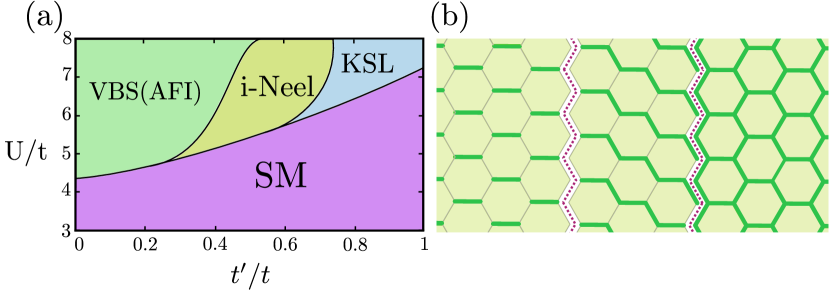
Figure 1: (a) Phase Diagram of the Kitaev-Hubbard Model. Initially, the system resides in the semi-metallic (SM) phase. As the Hubbard interaction strength increases, a phase transition occurs, driving the system into the Mott insulator (MI) phase. Within the MI phase, the system exhibits an initial presence in the Valence Bond Solid (VBS) phase, characterized by $g_{\gamma}$ being non-zero only along one of nearest neighbours, indicative of valence bond solid formation. The insertion of magnetic instability identifies this phase as the antiferromagnetic insulator(AFI). Subsequently, with an increase in asymmetry ($t^{\prime}/t$), the system undergoes a phase transition, during which $g_{\gamma}$ remains non-zero along one of nearest neighbour. Examination of magnetic fluctuations reveals an incommensurate Neel (i-Neel) order in this phase. Finally, the system enters a novel phase where $g_{\gamma}$ is non-zero along all three spatial directions. This phase smoothly connects to the regime characterized by $t^{\prime}/t=1$ and large $U$, where the system manifests as a Kitaev spin liquid. Notably, in this phase, spinons are gapless, signifying a gapless Kitaev spin liquid. (b) Visualization of $g_{\gamma}$ values in distinct phases of Kitaev-Hubbard model after Mott transition. Non-zero $g_{\gamma}$ values are represented by green lines.

The transverse Ising field Hamiltonian illustrates two distinct phases in the system. With an increase in the transverse field strength beyond a critical point $U_{c}$, the system undergoes a quantum phase transition from a ferromagnetic to a paramagnetic state. In the paramagnetic phase, we observe $\langle I_{i}^{x}\rangle=0$. Given that $I_{x}$ encapsulates the electron charge property, in this phase charge fluctuations are suppressed which leads to the Mott phase after the quantum phase transition. It can be demonstrated that the quasi-particle weight is given by $Z=4\langle I_{i}^{x}\rangle^{2}$, and, knowing that the Landau pseudo-particle weight becomes zero after the Mott transition, this depiction aligns perfectly with the Mott phase transition in the system. The $\mathbb{Z}_{2}$ slave-spin method facilitates a correspondence wherein the Mott phase transition is mapped onto transverse-field Ising transition. As depicted in Fig. 1(a), the system initially resides in the semi-metallic phase. With increasing coulomb repulsion strength, $U$, for different values of $t^{\prime}$, the system undergoes a transition into the Mott phase.

After the Mott phase transition, the dominant excitations in the system are spinons, and the system is described by gapless spinons without charge degrees of freedom represented by $f_{i,s}$. The fermionic sector of the mean-filed Hamiloian (7), contains four energy bands where two middle ones are connected at the Dirac points, with the distinction that the hopping coefficients are asymmetric. The values of these hopping coefficients, i.e., $g_{ij}$, represent spin correlations in the Ising model. It’s crucial to mention that here, $g_{ij}$ is computed for neighboring sites. Consequently, one anticipates a decrease in these values within the Mott phase, although they do not necessarily reach zero. Furthermore, $g_{ij}$ acts as a renormalization factor for the fermionic hoppings in $H_{\rm MF}$, being inversely proportional to the effective mass of the fermions $g_{i,j}=\frac{m}{m^{*}}$.

Considering the various values that $g_{\gamma}$ takes after the Mott phase transition, the system resides in different phases. As illustrated in Fig.1(b), in the Valence Bond Solid (VBS) phase, $g_{\gamma}$ becomes non-zero only for one of nearest neighbors. This implies that spinons exclusively hop to one of their adjacent sites, leading to the formation of a solid bond order. Subsequently, as the parameter $t^{\prime}$ increases, the system transitions into a phase where $g_{\gamma}$ is non-zero in one direction and zero in the other two directions. In this regime, the system enters a weakly frustrated phase. Ultimately, the system will manifest a phase where the $g_{\gamma}$ parameter is non-zero in all three directions. This phase continuously connects to the Kitaev spin liquid in the limit of large $U$ and $t^{\prime}=1$. Furthermore, owing to the gapless nature of the spinon spectrum $H_{f}$, this phase represents a gapless spin liquid.

Despite the fact that the time-reversal symmetry is broken in the original Hamiltonian, the mean field approximation we applied does not introduce magnetic instabilities in the system, preventing the observation of magnetic orderings in this approximation. However, given that for large values of $U$ and small $t^{\prime}$, the system is effectively described by an antiferromagnetic Heisenberg model (see (2)), we anticipate the VBS phase to exhibit antiferromagnetic ordering beyond the mean-field approximation. In the subsequent section, we elucidate the magnetic phases of the system by introducing spin fluctuations.

IV Magnetically ordered phases and magnetic fluctuations

To investigate the magnetic phases in this model, we express the Hubbard interaction in terms of spin fluctuations as follows

$$H_{U}=\sum_{j}\left(-\frac{U}{6}\sigma_{j}^{2}+\frac{U}{4}\right)$$ (9)

where $\sigma_{j}=c_{j,\alpha}^{\dagger}\sigma_{\alpha,\beta}c_{j,\beta}$. By employing the Hubbard-Stratonovich transformation, the total action of the system in terms of two effective fields, ferromagnetic $\phi_{F,j}$ and antiferromagnetic $\phi_{AF,j}$ in each unit cell, can be expressed as

$$S[\bar{c},c,\phi_{AF},\phi_{F}]=\int_{0}^{\beta}d\tau\Big{[}\sum_{\mathbb{k}}c_{\mathbb{k}}^{\dagger}(\partial_{\tau}+H_{\mathbb{k}})c_{\mathbb{k}}-\sum_{j}\phi_{F,j}\cdot(\mathbb{\sigma_{j,A}}+\mathbb{\sigma_{j,B}})+\frac{3}{U}\sum_{j}{\phi}^{2}_{F,j}-\sum_{j}\phi_{AF,j}\cdot(\mathbb{\sigma_{j,A}}-\mathbb{\sigma_{j,B}})+\frac{3}{U}\sum_{j}\phi_{AF,j}^{2}\Big{]}.$$ (10)

Here, $H_{\mathbf{k}}$ represents the non-interacting Hamiltonian of the system. For large values of $U$ and $t^{\prime}=0$, the effective spin model of the system will be a Heisenberg model with a ground state of antiferrromagnetism. Therefore, it seems that the mean-field approximation with antiferrromagnetic order can provide a suitable effective field for small $t^{\prime}$. By minimizing the action with respect to the uniform mean fields $\phi_{F,j}=\phi_{F}=0$ and $\phi_{AF,j}=\phi_{AF}=M\hat{z}$, the antiferrromagnetic order parameter is given by

$$M=\frac{U}{6}\left\langle\left(\sigma_{j,A}^{z}-\sigma_{j,B}^{z}\right)\right\rangle.$$ (11)

As depicted in Figure 2(a), the system lacks any magnetic order for small values of $t^{\prime}$ and $U$, residing in a semi-metallic phase. However, with increasing $U$, the system undergoes a transition into an antiferrromagnetic phase.

In the subsequent analysis, we further explore the magnetic phase by examining the spin fluctuations around the mean-field. The magnetic fluctuations within the Random Phase Approximation (RPA) are described by the following expression

$$\langle\sigma_{\mathbb{q}}^{\mu}\sigma_{\mathbb{-q}}^{\nu}\rangle=\frac{1}{I^{2}}\Bigg{\{}\Big{[}I_{m}^{-1}-\chi_{0}(\mathbb{q})\Big{]}^{-1}-I_{m}\Bigg{\}}_{\mu,\nu}.$$ (12)

Here, $\chi_{0}(\mathbb{q})$ denotes the bare susceptibility, $I=U/6$,

$$I_{m}=\left(\begin{matrix}I&0&0\\ 0&2I&0\\ 0&0&2I\end{matrix}\right),$$ (13)

$\sigma_{\mathbb{q}}^{\mu}=\sigma_{\mathbb{q},A}^{\mu}-\sigma_{\mathbb{q},B}^{\mu}$ and $\mu,\nu={z,+,-}$ represent the longitudinal and transverse directions. In Figure 2, static magnetic excitation spectrum for different values of $t^{\prime}$ and fixed $U=3.5$, around the $\Gamma$ point is shown. As illustrated, for $t^{\prime}=0$, excitations at the $\Gamma$ point are gapless. With an increase in $t^{\prime}$, two peaks emerge around the $\Gamma$ point, indicating the system’s transition to an incommensurate antiferromagnetic phase. Further increases in $t^{\prime}$ lead to fully gapped excitation spectra, signifying another phase transition. At $t^{\prime}=0.9$, the antiferrromagnetic order completely diminishes. In this regime the magnons excitations are the same and gapped in both transverse and longitudinal directions.Consequently, the system undergoes a progression from an initial semi-metal to an antiferrromagnetic phase and further evolves into an incommensurate Neel order with increased asymmetry. These results support the conclusion that the identified VBS state, utilizing $\mathbb{Z}_{2}$ slave spins, corresponds to a antiferrromagnetic phase, succeeded by the entry into the i-Neel order.

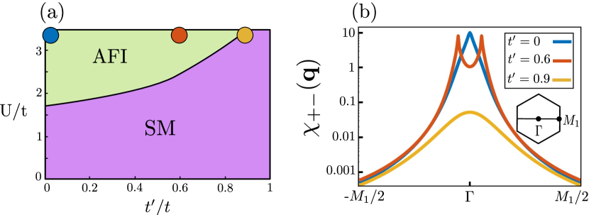
Figure 2: (a) Antiferromagnetic order parameter, $M$, in terms of $t^{\prime}/t$ and $U/t$. For small $U/t$ the system is in a semimetal phase with $M=0$. As both $U$ and $t^{\prime}$ increase, the order parameter attains a nonzero value, signaling a transition to the antiferromagnetic insulating (AFI) phase. (b)Transverse static spectral function of antiferromagnetic excitations around the $\Gamma$ point within the Random Phase Approximation (RPA), considering different $t^{\prime}$ values with $U=3.5$. Transverse fluctuations at $t^{\prime}=0$ exhibit a peak at the $\Gamma$ point, indicative of an antiferromagnetic phase with two degenerate magnon modes. As the asymmetry ($t^{\prime}$) increases, the degeneracy is lifted, revealing two distinct peaks around the $\Gamma$ point. This behavior signifies an incommensurate antiferromagnetic phase. Further increase in $t^{\prime}$ (specifically, $t^{\prime}=0.9$) introduces spin-wave gaps, indicative of a phase transition in the system.

V Quantum Monte Carlo Simulation

In order to go beyond the mean-field approximation and treat the model Hamiltonian in Eq. (II) exactly, we employ the auxiliary field QMC method [21] to study the dynamical spin susceptibility of the model in the strong $U$ limit. The QMC method is based on discretizing the evolution operator in calculating the expectation value $\left\langle O\right\rangle=\frac{{\rm Tr}\left[e^{-\beta H}O\right]}{{\rm Tr}\left[e^{-\beta H}\right]}$, using a symmetric Suzuki-Trotter decomposition scheme on the imaginary time interval $(0,\beta=M\Delta\tau)$, where $M$ is the number of the time slices along the imaginary time axis. The electron-electron interactions can be included in the calculations in an exact manner by employing an appropriate Hirsch-Hubbard-Stratonovich transformation [22]. Although the finite value of $\Delta\tau$ will induce a systematic error in the numerical results on the order of $O(\Delta\tau^{2})$, we found that $\Delta\tau=1/10$ will give reliable and converged results. We consider a lattice with $L\times L$ unit cells ($2L^{2}$ lattice points) and perform QMC calculations for inverse temperatures equal to $\beta=8$. We confirmed that this temperature ($T=1/8$) is low enough to achieve the convergence in the spin-spin correlations.

In this section, we focus on $U=5$ to investigate the claims that close to this value of $U$, a quantum spin liquid as well as a zigzag spin order phases are present for $t^{\prime}>1$ [12, 15, 14, 17]. Although, the KHM suffers from the fermionic sign problem and its average sign diminishes quickly upon increasing $t^{\prime}$ beyond unity, for the system size and the temperatures studied in this work, it remains above $0.2$ (see Fig. 3). However, we used increased samplings and thousands of independent Markov chains to keep the statistical error bars negligible and circumvent the fermionic sign problem to achieve virtually exact results. Furthermore, we observed that the recently proposed adiabatic QMC approach [23] can significantly reduce the statistical noise for the current model Hamiltonian and has been employed in this work.

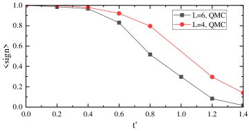
Figure 3: Average sign of QMC calculations as a function of $t^{\prime}$ for $\beta=8$, $U=5$ and $L=4$, $6$.

In the following we study the dynamical spin susceptibility which is defined by

$$\chi({\bf q},\omega)=\frac{i}{3}\sum_{\alpha=x,y,z}\frac{1}{L^{2}}\sum_{m,n}e^{i{\bf q}.({\bf r}_{m}-{\bf r}_{n})}\int_{0}^{\infty}dte^{i\omega t}\left\langle\left[S_{m}^{\alpha}(t),S_{{\bf n}}^{\alpha}\right]\right\rangle,$$ (14)

where $m,n$ runs over all lattice points. We present our QMC results for $L=4$ ($32$ site) and $L=6$ ($72$ sites) in Figs.4 and 5, respectively. For small values of $t^{\prime},$ the system is in AF Mott phase where the spin susceptibility is gapless around $\Gamma^{\prime}$ point as it is seen in Figs.4 and 5(a). This behavior is also obvious in the static spin susceptibilities shown in Figs.4 and 5(b) where the maximum value of the static dynamical susceptibility happens at $\Gamma^{\prime}$ points. Moreover, the real space correlation function in $z$ direction in Figs.4 and 5(c) also shows AF ordering. On the other hand, the dynamical spin susceptibility shown in the second and third lines of Figs.4 and 5 for $t^{\prime}\sim 0.9$ and $1.1$, exhibits broad small spectral gap between $\Gamma$ and $M_{1}$ points which is a signature that the system is in spin liquid phase. The results for $t^{\prime}=1.35$ are only shown for $L=4$ in Fig.4 because of the poor average sign for the results with $L=6$. Here, the system is in the zigzag order where the spectra is mainly gapless around $M$ points.

In order to identify the boundary between AFM, QSL and the zigzag phases we use the correlation ratio defined as

$$C_{{\bf k}}=\frac{\chi_{z}({\bf q}={\bf k})}{\chi_{z}({\bf q}={\bf k}^{*})},$$ (15)

where ${\bf k}^{*}$ is the nearest point to ${\bf k}$ in the reciprocal lattice. Fig.6 shows the correlation ratios which are calculated at the points ${\bf k}=\Gamma^{\prime}$ and ${\bf k}=M_{1}$. It is seen the for $0\leq t^{\prime}\leq 0.87$, the correlation ratio for ${\bf k}=\Gamma^{\prime}$ is greater than unity while $C_{M_{1}}<1$. This means that the the static spin spin susceptibility is peaked only at the $\Gamma^{\prime}$ point. We consider this observation as a signature of the AFM phase. On the other hand, for $t^{\prime}\geq 1.11$, we obtain $C_{M_{1}}>1$, while $C_{\Gamma^{\prime}}<1,$which can be considered as a signature of the zigzag order. The region in between these $t^{\prime}$values where both correlation ratios are less than unity can be identified as the QSL phase.

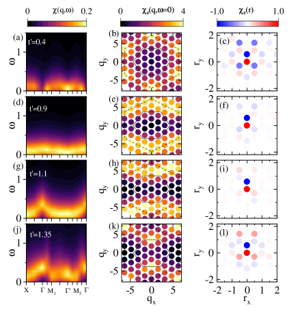
Figure 4: Left panels: Dynamical spin susceptibility, middle panels: Static spin susceptibility, and right panels: Real space spin-spin correlation function for $L=4$, $U=5$ and $\beta=8$. Different rows show results for $t^{\prime}=0.4,0.9$, $1.1$ and $1.35$, respectively.

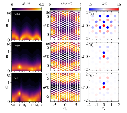
Figure 5: Left panels: Dynamical spin susceptibility, middle panels: Static spin susceptibility, and right panels: Real space spin-spin correlation function for $L=6$, $U=5$ and $\beta=8$. Different rows show results for $t^{\prime}=0.4,0.9$ and $1.1$, respectively.

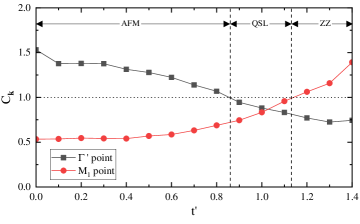
Figure 6: Correlation ratio $C_{{\bf k}}$ calculated at ${\bf k}=\Gamma^{\prime}$ and ${\bf k}=M_{1}$ points. Here $L=4$, $\beta=8$ and $U=5$

VI conclusions

Our work is mainly motivated by recent experiments on layered materials such as iridates and $\alpha$-RuCl₃, where the magnetic ions with strong correlations are sitting on the vertices of a honeycomb lattice. A prototype model could be Hubbard model in presence of spin-orbit coupling. In this article, we investigated the existence of a spin liquid in a model of a strongly correlated fermionic system with asymmetric spin-orbit couplings, known as the Kitaev-Hubbard model. Employing the $\mathbb{Z}_{2}$ slave spin method, a Mott transition is signaled by vanishing the quasiparticle weight. We further obtained the full phase diagram of the model and demonstrate that, in the regime of intermediate Hubbard interactions and relatively strong spin-orbit couplings, the model exhibits a gapless spin liquid phase. In the Mott phase, as the strength of the spin-orbit coupling inceases, multiple phase transitions occur. While at small values of spin-orbit coupling, the model is antiferromagnetically ordered, the intermediate values yields an incommensurate Neel order. For stronger spin-orbit couplings, the system enters a Kitaev spin liquid phase with no symmetry breaking. To deepen our exploration, we employ quantum Monte Carlo method to investigate the dynamical susceptibility of the system, yielding results in agreement with analytical predictions. The observation of the Kitaev spin liquid state in this model may contribute to our understanding of materials like $\alpha$-RuCl₃, which is shown to be in proximate to Kitaev spin liquid.

References

- Anderson [1973] P. Anderson, Resonating valence bonds: A new kind of insulator?, Materials Research Bulletin 8, 153 (1973).
- Anderson [1987] P. W. Anderson, The resonating valence bond state in and superconductivity, Science 235, 1196 (1987), https://www.science.org/doi/pdf/10.1126/science.235.4793.1196 .
- Nayak et al. [2008] C. Nayak, S. H. Simon, A. Stern, M. Freedman, and S. Das Sarma, Non-abelian anyons and topological quantum computation, Rev. Mod. Phys. 80, 1083 (2008).
- Banerjee et al. [2016] A. Banerjee, C. A. Bridges, J.-Q. Yan, A. A. Aczel, L. Li, M. B. Stone, G. E. Granroth, M. D. Lumsden, Y. Yiu, J. Knolle, S. Bhattacharjee, D. L. Kovrizhin, R. Moessner, D. A. Tennant, D. G. Mandrus, and S. E. Nagler, Proximate kitaev quantum spin liquid behaviour in a honeycomb magnet, Nature Materials 15, 733 (2016).
- Kasahara et al. [2018] Y. Kasahara, T. Ohnishi, Y. Mizukami, O. Tanaka, S. Ma, K. Sugii, N. Kurita, H. Tanaka, J. Nasu, Y. Motome, T. Shibauchi, and Y. Matsuda, Majorana quantization and half-integer thermal quantum hall effect in a kitaev spin liquid, Nature 559, 227 (2018).
- Banerjee et al. [2018] A. Banerjee, P. Lampen-Kelley, J. Knolle, C. Balz, A. A. Aczel, B. Winn, Y. Liu, D. Pajerowski, J. Yan, C. A. Bridges, A. T. Savici, B. C. Chakoumakos, M. D. Lumsden, D. A. Tennant, R. Moessner, D. G. Mandrus, and S. E. Nagler, Excitations in the field-induced quantum spin liquid state of -rucl3, npj Quantum Materials 3, 8 (2018).
- Kim et al. [2009] B. J. Kim, H. Ohsumi, T. Komesu, S. Sakai, T. Morita, H. Takagi, and T. Arima, Phase-sensitive observation of a spin-orbital mott state in , Science 323, 1329 (2009), https://www.science.org/doi/pdf/10.1126/science.1167106 .
- Jackeli and Khaliullin [2009] G. Jackeli and G. Khaliullin, Mott insulators in the strong spin-orbit coupling limit: From heisenberg to a quantum compass and kitaev models, Phys. Rev. Lett. 102, 017205 (2009).
- Singh et al. [2012] Y. Singh, S. Manni, J. Reuther, T. Berlijn, R. Thomale, W. Ku, S. Trebst, and P. Gegenwart, Relevance of the heisenberg-kitaev model for the honeycomb lattice iridates , Phys. Rev. Lett. 108, 127203 (2012).
- Kitagawa et al. [2018] K. Kitagawa, T. Takayama, Y. Matsumoto, A. Kato, R. Takano, Y. Kishimoto, S. Bette, R. Dinnebier, G. Jackeli, and H. Takagi, A spin-orbital-entangled quantum liquid on a honeycomb lattice, Nature 554, 341 (2018).
- Duan et al. [2003] L.-M. Duan, E. Demler, and M. D. Lukin, Controlling spin exchange interactions of ultracold atoms in optical lattices, Phys. Rev. Lett. 91, 090402 (2003).
- Hassan et al. [2013] S. R. Hassan, P. V. Sriluckshmy, S. K. Goyal, R. Shankar, and D. Sénéchal, Stable algebraic spin liquid in a hubbard model, Phys. Rev. Lett. 110, 037201 (2013).
- Faye et al. [2014] J. P. L. Faye, D. Sénéchal, and S. R. Hassan, Topological phases of the kitaev-hubbard model at half filling, Phys. Rev. B 89, 115130 (2014).
- Dong et al. [2023] S. Dong, H. Zhang, C. Wang, M. Zhang, Y.-J. Han, and L. He, A possible quantum spin liquid phase in the kitaev-hubbard model, Chinese Physics Letters 40, 126403 (2023).
- Liang et al. [2014] L. Liang, Z. Wang, and Y. Yu, Distinct-symmetry spin-liquid states and phase diagram of the kitaev-hubbard model, Phys. Rev. B 90, 075119 (2014).
- Huber and Rüegg [2009] S. D. Huber and A. Rüegg, Dynamically generated double occupancy as a probe of cold atom systems, Phys. Rev. Lett. 102, 065301 (2009).
- Sato and Assaad [2021] T. Sato and F. F. Assaad, Quantum monte carlo simulation of generalized kitaev models, Physical Review B 104, L081106 (2021).
- Florens and Georges [2004] S. Florens and A. Georges, Slave-rotor mean-field theories of strongly correlated systems and the mott transition in finite dimensions, Physical Review B 70, 035114 (2004).
- Mardani et al. [2011] M. Mardani, M.-S. Vaezi, and A. Vaezi, Slave-spin approach to the strongly correlated systems, arXiv preprint arXiv:1111.5980 (2011).
- Hassan and de’ Medici [2010] S. R. Hassan and L. de’ Medici, Slave spins away from half filling: Cluster mean-field theory of the hubbard and extended hubbard models, Phys. Rev. B 81, 035106 (2010).
- White et al. [1989] S. R. White, D. J. Scalapino, R. L. Sugar, E. Loh, J. E. Gubernatis, and R. T. Scalettar, Numerical study of the two-dimensional hubbard model, Physical Review B 40, 506 (1989).
- Hirsch [1983] J. E. Hirsch, Discrete hubbard-stratonovich transformation for fermion lattice models, Physical Review B 28, 4059 (1983).
- Vaezi et al. [2021] M.-S. Vaezi, A.-R. Negari, A. Moharramipour, and A. Vaezi, Amelioration for the sign problem: An adiabatic quantum monte carlo algorithm, Physical Review Letters 127, 217003 (2021).