Projected Langevin Monte Carlo algorithms in non-convex and super-linear setting

Abstract

It is of significant interest in many applications to sample from a high-dimensional target distribution $\pi$ with the density $\pi(\text{d}x)\propto e^{-U(x)}(\text{d}x)$, based on the temporal discretization of the Langevin stochastic differential equations (SDEs). In this paper, we propose an explicit projected Langevin Monte Carlo (PLMC) algorithm with non-convex potential $U$ and super-linear gradient of $U$ and investigate the non-asymptotic analysis of its sampling error in total variation distance. Equipped with time-independent regularity estimates for the corresponding Kolmogorov equation, we derive the non-asymptotic bounds on the total variation distance between the target distribution of the Langevin SDEs and the law induced by the PLMC scheme with order $\mathcal{O}(h|\ln h|)$. Moreover, for a given precision $\epsilon$, the smallest number of iterations of the classical Langevin Monte Carlo (LMC) scheme with the non-convex potential $U$ and the globally Lipshitz gradient of $U$ can be guaranteed by order ${\mathcal{O}}\big{(}\tfrac{d^{3/2}}{\epsilon}\cdot\ln(\tfrac{d}{\epsilon})\cdot\ln(\tfrac{1}{\epsilon})\big{)}$. Numerical experiments are provided to confirm the theoretical findings.

AMS subject classification: 60H35, 65C05, 65C30.

Key Words: Langevin Monte Carlo sampling, total variation distance, non-convex potential, projected scheme, Kolmogorov equations.

1 Introduction

Sampling from a high-dimensional ($d\gg 1$) target distribution $\pi$ plays a crucial role in various fields such as Bayesian inference, statistical physics, machine learning and computational biology and has been a subject of recent intensive research efforts. For example, evaluating the expectation of some functional $\phi$ with respect to $\pi$:

$$\pi(\phi):=\int_{\mathbb{R}^{d}}\phi(x)\pi(\text{d}x),$$ (1.1)

is of great interests in applications in the area of Bayesian statistics. A typical approach of sampling is to set the target measure $\pi$ as the invariant measure of the stochastic differential equations (SDEs) and undertake an appropriate numerical scheme that discretizes such SDEs in time. More precisely, we consider a class of sampling methods based on the following overdamped Langevin stochastic differential equations (SDEs) of Itô type:

$$\text{d}X_{t}=-\nabla U(X_{t})\,\text{d}t+\sqrt{2}\,\text{d}W_{t},\quad X_{0}=x_{0},\quad t>0,$$ (1.2)

where $W_{\cdot}=\left(W_{1,\cdot},\dots,W_{d,\cdot}\right)^{T}:[0,\infty)\times\Omega\rightarrow\mathbb{R}^{d}$ denotes the $\mathbb{R}^{d}$-valued standard Brownian motion with respect to $\left\{\mathcal{F}_{t}\right\}_{t\geq 0}$. and the initial data $x_{0}:\Omega\rightarrow\mathbb{R}^{d}$ is assumed to be $\mathcal{F}_{0}$-measurable. Under certain conditions, the dynamics of (1.2) agrees with the distribution $\pi$ with the density $\pi(\text{d}x)\propto e^{-U(x)}(\text{d}x)$. To asymptotically sample from $\pi$ admitted by (1.2), one notable example is the unadjusted Langevin Monte Carlo (LMC for short) algorithm, which also corresponds to the well-known Euler-Maruyama scheme of the Langevin SDE (1.2), denoted by $\{\widetilde{Y}_{n}\}_{n\geq 0}$ as

$$\widetilde{Y}_{n+1}=\widetilde{Y}_{n}-\nabla U\big{(}\widetilde{Y}_{n}\big{)}h+\sqrt{2h}\xi_{n+1},\quad\widetilde{Y}_{0}=x_{0},$$ (1.3)

where $h\in(0,1)$ represents the uniform timestep and $\xi_{k}=(\xi_{1,k},\dots,\xi_{d,k})^{T}$, $k\in\mathbb{N}$, are i.i.d standard $d$-dimensional Gaussian vectors.

Non-asymptotic analysis focuses on the explicit dependency of the error with respect to the algorithm parameters, e.g., step size, rather than explaining the asymptotic behavior as the algorithm iterates to infinity or the step size tends to zero. Non-asymptotic convergence analysis for the LMC algorithm (1.3) is typically investigated with

(i) globally Lipschitz condition: there exists a positive constant $\bar{L}>0$ such that

$$\|\nabla U(x)-\nabla U(y)\|\leq\bar{L}\|x-y\|,\quad\forall x,y\in\mathbb{R}^{d},\,\text{ and }$$ (1.4)

(ii) strongly-convex condition: there exists a positive constant $\widetilde{L}>0$ such that

$$\left\langle x-y,\nabla U(x)-\nabla U(y)\right\rangle\geq\widetilde{L}\|x-y\|^{2},\quad\forall x,y\in\mathbb{R}^{d}.$$ (1.5)

In recent years, working with condition (i) and (ii), non-asymptotic error analysis between the target distribution and the law of the LMC algorithm under various metrics, such as the Wasserstein distance and the total variation distance has been well established (see [9, 8, 10]).

Except for a few rare cases, it is extremely tough for the Langvin SDE (1.2) to satisfy either condition (i) or (ii). A commonly used counterexample in quantum mechanics is the double-well potential presented in Example 2.5. What if the drift $\nabla U$ grows superlinearly? Conventional LMC algorithm loses its powers when attempting to sample from the target distribution inherited by (1.2). For example, as claimed by [13, 19], for a large class of SDEs with super-linear growth coefficients, the Euler-Maruyama scheme (1.3) leads to divergent numerical approximations in both finite and infinite time intervals. Therefore, a convergent numerical algorithm for the Langevin SDEs (1.2) with non-globally Lipschitz drift is necessary. Recent years have witnessed a considerable growth in construction and analysis of convergent schemes with SDEs in the non-globally Lipschitz setting (see [25, 14, 16, 23, 26, 1, 2, 24]). Moreover, to deal with the super-linear drift of the Langevin SDEs (1.2), authors in [4] used a tamed Langevin algorithm to obtain the non-asymptotic error bounds on 2-Wasserstein distance and total variation distance.

Beside the challenge of the super-linear drift, relaxing the strongly-convex potential, i.e. condition (ii), may lead to possible collapse of the classical method in the non-asymptotic error analysis [18], where the contractivity condition can be replaced by a contractivity at infinity condition (see Assumption 2.2). Recently, working on such a relaxed condition and demonstrating the non-asymptotic error analysis of the corresponding Langevin SDEs (1.2) have indeed gained appreciable attention (see [21, 18, 20] for example). Nevertheless, it is worth mentioning that a majority of existing works investigate this topic via the Wasserstein distance error bounds. In [18], authors obtained the non-asymptotic upper bound on 1-Wasserstein distance and 2-Wasserstein distance of order $1/2$ and $1/4$, respectively, under globally Lipschitz condition. If the Lipschitz condition is weakened by a polynomial growth condition, authors in [20] improved the 1-Wasserstein error bound and the 2-Wasserstein error bound with respective convergence order of $1$ and $1/2$.

In this paper, we investigate the non-asymptotic convergence of the target distribution admitted by (1.2) in total variation distance (2.7)-(2.10) in non-convex and non-globally Lipschitz setting (see Assumptions 2.1, 2.2 and 2.4 below). The setting of total variation distance allows us to consider bounded and measurable function $\phi\in B_{b}(\mathbb{R}^{d})$ in (1.1). Classical examples include the indicator function and the step function (see (6.2)). As far as we know, the investigation of approximation errors in weak approximations of (1.1) without fulfilling conditions (i) and (ii) is still in its initial phases. To recover the convergence for the Langevin SDEs (1.2) with super-linear growing nonlinearities, we propose a projected Langevin Monte Carlo (PLMC) algorithm (cf. (2.17)) with a uniform timestep, which reduces to the classical LMC algorithm (1.3) for the Langevin SDEs (1.2) with a Lipschitz continuous drift. This fact paves the way to analyzing the smallest number of iterations of the LMC scheme (1.3) required to approach the target distribution inherited by (1.2) on the total variation distance with given precision, also known as the mixing time, under Lipschitz condition, which has been remaining an active field [15, 6] in recent years.

Non-asymptotic bounds on the total variation distance between the law of the PLMC algorithm and the target distribution boil down to the weak error analysis of the PLMC scheme and the Langevin SDEs (1.2) for some test functions $\phi\in B_{b}(\mathbb{R}^{d})$, which can be derived based on the corresponding Kolmogorov equation (4.2) of SDEs (1.2). However, one may encounter two major obstacles. The first one is to get a couple of a priori estimates that are independent of time and stepsize, including the uniform moment bounds of the PLMC scheme (2.17) and the time-independent regularity estimates of the Kolmogorov equation, which is very challenging due to the loss of condition (ii) and the non-smooth test function. Another one is the discontinuity of the proposed PLMC algorithm (2.17), which results in further difficulties in handling the weak error via the Kolmogorov equation. Different techniques are used to circumvent these difficulties. Discrete arguments are adopted to obtain the uniform moment bounds of the PLMC algorithm (2.17) (see the proof of Lemma 3.4). Moreover, the Bismut-Elworthy-Li formula (see Lemma 4.3) combined with the Markov property of the transition semigroup $u(\cdot,\cdot)$ (4.1) are used to derive the time-independent regularity estimates of the Kolmogorov equation (see Section 4). To handle the discontinuity of the PLMC algorithm (3.8), we introduce the continuous-time version (see (5.2)) at each step to fully exploit the Kolmogorov equation (see (4.2)).

Moving on to the error analysis, given any terminal time $T\in(0,\infty)$ such that $Nh=T$, $N\in\mathbb{N}$, we separate the error $\big{|}\mathbb{E}\left[\phi(Y^{x_{0}}_{N})\right]-\mathbb{E}\left[\phi(X^{x_{0}}_{T})\right]\big{|}$, i.e., $\big{|}\mathbb{E}\left[u(T,x_{0})\right]-\mathbb{E}\left[u(0,Y^{x_{0}}_{N})\right]\big{|}$ based on the associated Kolmogorov equation (see (4.2)) into two parts as $J_{1}$ and $J_{2}$ in (5.8). The first part $J_{1}$ is of order $1$, which can be considered as a direct consequence of the time-independent regularity of $u(t,\cdot)$ (see Theorem 4.4) and the convergence of the projected operator $\mathscr{P}(\cdot)$ (see Lemma 5.2). Depending on the continuous version of the PLMC algorithm (5.2), the Kolmogorov equation and the Itô formula, the second error term $J_{2}$ can be proved to be $\mathcal{O}(h|\ln h|)$ (see Theorem 5.3 and its proof for more details). Directly from Theorem 2.6, one can show that, the smallest number of iterations of the LMC scheme (1.3) is of order ${\mathcal{O}}\big{(}\tfrac{d^{3/2}}{\epsilon}\cdot\ln(\tfrac{d}{\epsilon})\cdot\ln(\tfrac{1}{\epsilon})\big{)}$, for the drift $f$ being contractivity at infinity and the globally Lipshitz continuity (see Remark 2.8).

We summarize our main contributions as follows:

• A projected Langevin Monte Carlo algorithm, capable of dealing with super-linear systems and covering the classical Langevin Monte Carlo algorithm, is presented.

• Non-asymptotic bounds on the total variation distance between the law of the PLMC algorithm and the target distribution, inherited by (1.2), is established for non-convex potential.

• The smallest number of iterations of the Langevin Monte Carlo scheme required to approach the target distribution, admitted by (1.2), in the total variation distance with given precision is shown in Lipschitz but non-convex setting.

The rest of this article is organized as follows. The next section formulates the primary setting and shows the main result of this paper. In Section 3, we present some a priori estimates of both SDE and the PLMC algorithm. Section 4 reveals the Kolmogorov equation and its regularity estimates. In Section 5, the time-independent weak error analysis between SDE and the PLMC scheme is given. Some numerical tests are shown to illustrate our theoretical findings in Section 6. Finally, the Appendix contains the detailed proof of several auxiliary lemmas.

2 Settings and main result

Throughout this paper, we use $\mathbb{N}$ to denote the set of all positive integers and let $d,m\in\mathbb{N}$, $T\in(0,\infty)$ be given. Let $\|\cdot\|$ and $\langle\cdot,\cdot\rangle$ denote the Euclidean norm and the inner product of vectors in $\mathbb{R}^{d}$, respectively. Adopting the same notation as the vector norm, we denote $\|A\|:=\sqrt{\operatorname{trace}(A^{T}A)}$ as the trace norm of a matrix $A\in\mathbb{R}^{d\times m}$. We use $\max\{a,b\}$ and $\min\{a,b\}$ for the maximum and minimum values of between $a$ and $b$ respectively. Given a filtered probability space $\left(\Omega,\mathcal{F},\{\mathcal{F}_{t}\}_{t\in[0,T]},\mathbb{P}\right)$, we use $\mathbb{E}$ to mean the expectation and $L^{r}(\Omega,\mathbb{R}^{d}),r\geq 1$, to denote the family of $\mathbb{R}^{d}$-valued random variables $\xi$ satisfying $\mathbb{E}[\|\xi\|^{r}]<\infty$. Moreover, we introduce a new notation $X^{x}_{t}$ for $t\in[0,\infty)$ denoting the solution of SDE (1.2) satisfying the initial condition $X^{x}_{0}=X_{0}=x$. In addition, denote by $C_{b}(\mathbb{R}^{d})$ (resp. $B_{b}(\mathbb{R}^{d})$ ) the Banach space of all uniformly continuous and bounded mappings (resp. Borel bounded mappings) $\varphi:\mathbb{R}^{d}\rightarrow\mathbb{R}$ endowed with the norm $\|\varphi\|_{0}=\sup_{x\in\mathbb{R}^{d}}|\varphi(x)|$.

For the vector-valued function $\textbf{u}:\mathbb{R}^{d}\rightarrow\mathbb{R}^{{\ell}}$, $\textbf{u}=(u_{(1)},\dots,u_{({\ell})})$, its first order partial derivative is considered as the Jacobian matrix as

$$D\mathbf{u}=\left(\begin{array}[]{ccc}\frac{\partial u_{(1)}}{\partial x_{1}}&\cdots&\frac{\partial u_{(1)}}{\partial x_{d}}\\ \vdots&\ddots&\vdots\\ \frac{\partial u_{(\ell)}}{\partial x_{1}}&\cdots&\frac{\partial u_{(\ell)}}{\partial x_{d}}\end{array}\right)_{\ell\times d}.$$ (2.1)

For any $v_{1}\in\mathbb{R}^{d}$, one knows $D(\mathbf{u})v_{1}\in\mathbb{R}^{\ell}$ and one can define $D^{2}\mathbf{u}(v_{1},v_{2})$ as

$$D^{2}\mathbf{u}(v_{1},v_{2}):=D\big{(}D(\mathbf{u})v_{1}\big{)}v_{2},\quad\forall v_{1},v_{2}\in\mathbb{R}^{d}.$$ (2.2)

In the same manner, one can define

$$D^{3}\mathbf{u}(v_{1},v_{2},v_{3}):=D\Big{(}D\big{(}D(\mathbf{u})v_{1}\big{)}v_{2}\Big{)}v_{3},\quad\forall v_{1},v_{2},v_{3}\in\mathbb{R}^{d},$$ (2.3)

and for any integer $k\geq 3$ the $k$-th order partial derivatives of the function u can be defined recursively. Given the Banach spaces $\mathcal{X}$ and $\mathcal{Y}$, we denote by $L(\mathcal{X},\mathcal{Y})$ the Banach space of bounded linear operators from $\mathcal{X}$ into $\mathcal{Y}$. Then the partial derivatives of the function u can also be regarded as the operators

$$D\textbf{u}(\cdot)(\cdot):\mathbb{R}^{d}\to L(\mathbb{R}^{d},\mathbb{R}^{\ell}),$$ (2.4)

$$D^{2}\textbf{u}(\cdot)(\cdot,\cdot):\mathbb{R}^{d}\to L(\mathbb{R}^{d},L(\mathbb{R}^{d},\mathbb{R}^{d}))\cong L(\mathbb{R}^{d}\otimes\mathbb{R}^{d},\mathbb{R}^{\ell})$$ (2.5)

and

$$D^{3}\textbf{u}(\cdot)(\cdot,\cdot,\cdot):\mathbb{R}^{d}\to L(\mathbb{R}^{d},L(\mathbb{R}^{d},L(\mathbb{R}^{d},\mathbb{R}^{d})))\cong L((\mathbb{R}^{d})^{\otimes 3},\mathbb{R}^{\ell}).$$ (2.6)

We remark that the partial derivatives of the scalar valued function can be covered by the special case $\ell=1$.

For any $k\in\mathbb{N}$, let $C^{k}_{b}(\mathbb{R}^{d})$ be the subspace of $C_{b}(\mathbb{R}^{d})$ consisting of all functions with bounded partial derivatives $D^{i}\varphi(x)$, $1\leq i\leq k$. In what follows, we use the letter $C$ to denote generic constants, independent of both the step size $h\in(0,1)$ and the dimension $d$. Also, let $\textbf{1}_{H}$ be the indicator function of a set $H$.

Further, the total variation distance between two Borel probability distributions $\mu_{1}$ and $\mu_{2}$ is defined by

$$\|\mu_{1}-\mu_{2}\|_{\text{TV}}:=\sup_{\varphi\in B_{b}(\mathbb{R}^{d}),\ \varphi\neq 0}\dfrac{\left|\int_{\mathbb{R}^{d}}\varphi(x)\mu_{1}(\text{d}x)-\int_{\mathbb{R}^{d}}\varphi(x)\mu_{2}(\text{d}x)\right|}{\|\varphi\|_{0}}.$$ (2.7)

Consequently, if $X$ is a $\mathbb{R}^{d}$-valued random variable, the probability distribution of $X$ is denoted by $\Pi(X)$. Then, the total variation distance between $\Pi(X)$ and any Borel probability distribution $\mu$ is given as,

$$\|\Pi(X)-\mu\|_{\text{TV}}:=\sup_{\varphi\in B_{b}(\mathbb{R}^{d}),\ \|\varphi\|_{0}\leq 1}\left|\mathbb{E}\left[\varphi(X)\right]-\int_{\mathbb{R}^{d}}\varphi(x)\mu(\text{d}x)\right|.$$ (2.8)

Recalling that for any $\varphi\in B_{b}(\mathbb{R}^{d})$, there exists a sequence $\varphi_{k}\in C_{b}(\mathbb{R}^{d})$, $k\in\mathbb{N}$ satisfying $\lim_{k\rightarrow\infty}\varphi_{k}(x)\rightarrow\varphi(x)$, for all $x\in\mathbb{R}^{d}$. Therefore, the total variation distance between two Borel probability distributions $\mu_{1}$ and $\mu_{2}$ has the representation as follows,

$$\|\mu_{1}-\mu_{2}\|_{\text{TV}} =\sup_{\varphi\in C_{b}(\mathbb{R}^{d}),\ \varphi\neq 0}\dfrac{\left|\int_{\mathbb{R}^{d}}\varphi(x)\mu_{1}(\text{d}x)-\int_{\mathbb{R}^{d}}\varphi(x)\mu_{2}(\text{d}x)\right|}{\|\varphi\|_{0}}$$ (2.9)

$$=\sup_{\varphi\in C_{b}(\mathbb{R}^{d}),\ \|\varphi\|\leq 1}\left|\int_{\mathbb{R}^{d}}\varphi(x)\mu_{1}(\text{d}x)-\int_{\mathbb{R}^{d}}\varphi(x)\mu_{2}(\text{d}x)\right|.$$

Moreover, for the probability distribution of $X$ and any Borel probability distribution $\mu$, one also has

$$\begin{split}\|\Pi(X)-\mu\|_{\text{TV}}&=\sup_{\varphi\in C_{b}(\mathbb{R}^{d}),\ \varphi\neq 0}\dfrac{\left|\mathbb{E}\left[\varphi(X)\right]-\int_{\mathbb{R}^{d}}\varphi(x)\mu(\text{d}x)\right|}{\|\varphi\|_{0}}\\ &=\sup_{\varphi\in C_{b}(\mathbb{R}^{d}),\ \|\varphi\|_{0}\leq 1}\left|\mathbb{E}\left[\varphi(X)\right]-\int_{\mathbb{R}^{d}}\varphi(x)\mu(\text{d}x)\right|.\end{split}$$ (2.10)

In the sequel, denote $f(x):=-\nabla U(x),\ \forall x\in\mathbb{R}^{d}$, as the negative gradient of the potential $U$ for convenience.

Subsequently, we set up a non-convex framework by stating some assumptions in order to establish the main result.

Assumption 2.1.

(Globally polynomial growth condition.) Assume the drift coefficient $f:\mathbb{R}^{d}\rightarrow\mathbb{R}^{d}$ of SDE (1.2) is twice continuously differentiable in $\mathbb{R}^{d}$, and there exists some constant $\gamma\in[1,\infty)$ such that,

$$\left\|D^{2}f(x)(v_{1},v_{2})\right\| \leq C(1+\|x\|)^{\gamma-2}\|v_{1}\|\cdot\|v_{2}\|,\quad\forall x,v_{1},v_{2}\in\mathbb{R}^{d}.$$ (2.11)

Note that Assumption 2.1 immediately implies

$$\left\|Df(x)v_{1}-Df(\tilde{x})v_{1}\right\| \leq C(1+\|x\|+\|\widetilde{x}\|)^{\gamma-2}\|x-\tilde{x}\|\cdot\|v_{1}\|,\quad\forall x,\tilde{x},v_{1}\in\mathbb{R}^{d},$$ (2.12)

$$\left\|Df(x)v_{1}\right\| \leq C(1+\|x\|)^{\gamma-1}\|v_{1}\|,\quad\forall x,v_{1}\in\mathbb{R}^{d},$$

which in turn yields

$$\left\|f(x)-f(\tilde{x})\right\| \leq C(1+\|x\|+\|\tilde{x}\|)^{\gamma-1}\|x-\tilde{x}\|,\quad\forall x,\tilde{x}\in\mathbb{R}^{d},$$ (2.13)

$$\left\|f(x)\right\| \leq C(1+\|x\|)^{\gamma},\quad\forall x\in\mathbb{R}^{d}.$$

In what follows, we formulate the contractivity at infinity condition as shown in [18].

Assumption 2.2.

(Contractivity at infinity condition.) For the drift coefficient $f:\mathbb{R}^{d}\rightarrow\mathbb{R}^{d}$ of SDE (1.2), there exist some positive constants $\widetilde{a}_{1}>\widetilde{a}_{2}>0$, $\mathcal{R}>0$ such that,

$$\left\langle x-y,f(x)-f(y)\right\rangle\leq\left(\widetilde{a}_{1}\mathbf{1}_{\|x-y\|\leq\mathcal{R}}-\widetilde{a}_{2}\right)\|x-y\|^{2},\quad\forall x,y\in\mathbb{R}^{d}.$$ (2.14)

Remark 2.3.

It is noteworthy that Assumption 2.2 implies a one-side Lipschitz condition of the drfit $f:\mathbb{R}^{d}\rightarrow\mathbb{R}^{d}$ as follows: there exists some positive constant $L>0$ such that

$$\left\langle x-y,f(x)-f(y)\right\rangle\leq L\|x-y\|^{2},\quad\forall x,y\in\mathbb{R}^{d}.$$ (2.15)

Further, we would like to present the dissipativity conditions for $f$.

Assumption 2.4.

For the drift coefficient $f:\mathbb{R}^{d}\rightarrow\mathbb{R}^{d}$, there exist some constants $a_{1},a_{2}>0$ such that

$$\left\langle x,f(x)\right\rangle\leq-a_{1}\|x\|^{\gamma+1}+a_{2},\quad\forall x\in\mathbb{R}^{d}.$$ (2.16)

Compared with the usual but strict strongly-convex condition on $U$ and the globally Lipschitz condition on $\nabla U$, Assumptions 2.1-2.4 enable us to accommodate for a much wider family of SDEs, especially for possible non-convex potentials. Here we give an example.

Example 2.5 (Double-well potential).

Consider $f(x)=x(1-\|x\|^{2})$, which is the negative gradient of the double-well potential $U(x)=\|x\|^{4}/4-\|x\|^{2}/2$. Such an $f$ violates (1.4) and (1.5) but satisfies Assumptions 2.1-2.4 with $\gamma=3$, $a_{1}=1/2$ and $a_{2}=1/2$, where the Young inequality $\|x\|^{2}\leq 1/2+\|x\|^{4}/2$ is used.

To obtain numerical approximations of the invariant measure allowed by such SDEs, even in high dimensions and without assuming strong convexity or Lipschitz continuity, we, therefore, propose a family of projected Langevin Monte Carlo (PLMC) algorithms as follows

$$\begin{split}\left\{\begin{array}[]{ll}Y_{n+1}=\mathscr{P}(Y_{n})+f\left(\mathscr{P}(Y_{n})\right)h+\sqrt{2h}\xi_{n+1},\\ Y_{0}=x_{0},\end{array}\right.\end{split}$$ (2.17)

where $\xi_{k}=(\xi_{1,k},\dots,\xi_{d,k})^{T}$, $k\in\mathbb{N}$, are i.i.d standard $d$-dimensional Gaussian vectors and $\mathscr{P}:\mathbb{R}^{d}\rightarrow\mathbb{R}^{d}$ denotes the projection operator given as

$$\mathscr{P}(x):=\begin{split}\left\{\begin{array}[]{ll}\min\big{\{}1,\vartheta(\tfrac{d}{h})^{1/2\gamma}\|x\|^{-1}\big{\}}x,\hskip 10.00002pt\text{for}\ \gamma>1,\\ x,\ \hskip 107.00012pt\text{for}\ \gamma=1,\end{array}\right.\end{split}\quad\forall x\in\mathbb{R}^{d},$$ (2.18)

with $\gamma$ being given in Assumption 2.1. Furthermore, note that the parameter $\vartheta\geq 1$, independent of the stepsize $h$ and the dimension $d$, is pre-determined to ensure that the numerical solutions of the PLMC scheme (2.17) will not be projected too often in the iteration, especially when dealing with a high-dimensional target distribution. In particular, when $\gamma=1$, then $\mathscr{P}=I$ is the identity operator.

The main result of this paper is formulated as follows,

Theorem 2.6.

(Main result – non-asymptotic bounds in the total variation distance.) Assume Assumptions 2.1, 2.2, 2.4. Let $\{X^{x_{0}}_{t}\}_{t\geq 0}$ and $\{Y^{x_{0}}_{n}\}_{n\geq 0}$ be the solutions of SDE (1.2) and the PLMC algorithm (2.17) with the initial state $X^{x_{0}}_{0}=Y^{x_{0}}_{0}=x_{0}$, respectively. Then the Langevin SDE $\{X^{x_{0}}_{t}\}_{t\geq 0}$ in (1.2) converges exponentially to a unique invariant measure, denoted by $\pi$, under total variation distance. Furthermore, let $h\in(0,\min\{1/a_{1},1\})$ be the uniform timestep with $a_{1}$ being shown in Assumption 2.4. Given any terminal time $T\in(0,\infty)$ such that $Nh=T$, $N\in\mathbb{N}$, for the super-linear drift $f$, i.e. $\gamma>1$,

$$\left\|\Pi(Y^{x_{0}}_{N})-\pi\right\|_{\text{TV}}\leq Ce^{-CNh}\left(1+\mathbb{E}\left[\|x_{0}\|^{2}\right]\right)+Cd^{\max\{3\gamma/2,2\gamma-1\}}h\left|\ln{h}\right|,$$ (2.19)

For the Lipschitz drift $f$, i.e. $\gamma=1$, let $\{\widetilde{Y}^{x_{0}}_{n}\}_{n\geq 0}$ be the solutions of the LMC algorithm (1.3) with the initial state $\widetilde{Y}^{x_{0}}_{0}=x_{0}$, then

$$\left\|\Pi(\widetilde{Y}^{x_{0}}_{N})-\pi\right\|_{\text{TV}}\leq Ce^{-CNh}\left(1+\mathbb{E}\left[\|x_{0}\|^{2}\right]\right)+Cd^{3/2}h\left|\ln{h}\right|.$$ (2.20)

Remark 2.7.

While completing this paper, we are aware of the work [17], where results analogous to (2.20) in Theorem 2.6 were obtained with a sequence of decreasing step sizes via Malliavin calculus under the contractivity at infinity condition on the Hölder continuous drift $f$. Instead, the main focus of this paper is the analysis of the total variation distance with super-linearly growing continuous drift $f$.

Remark 2.8.

Regarding the smallest number of iterations, i.e. mixing time, of the LMC scheme required to approximate the target measure of the Langevin SDE (1.2), it can be deduced from (2.20) of Theorem 2.6 that, to achieve a given precision level $\epsilon>0$, a required number of iterations is of order ${\mathcal{O}}\big{(}\tfrac{d^{3/2}}{\epsilon}\cdot\ln(\tfrac{d}{\epsilon})\cdot\ln(\tfrac{1}{\epsilon})\big{)}$. The proof is straightforward and postponed to Appendix D. To the best of our knowledge, this is the first result considering mixing time of the LMC algorithm under the total variation distance in non-convex setting.

3 Preliminary results

3.1 A priori estimates of the Langevin SDE

We begin with the lemma concerning the uniform moments estimate of $\{X_{t}\}_{t\geq 0}$, defined by (1.2).

Lemma 3.1.

(Uniform moment bounds of the Langevin SDE.) Let the solution of the Langevin SDE, denoted by $\{X_{t}\}_{t\geq 0}$ in (1.2), satisfy Assumptions 2.1, 2.2 and 2.4. Then, for some constant $c\in(0,a_{1})$ with $a_{1}$ being given in Assumption 2.4 and any $p\in[1,\infty)$

$$\mathbb{E}\left[\left\|X_{t}\right\|^{2p}\right]\leq e^{-cpt}\mathbb{E}\left[\|x_{0}\|^{2p}\right]+Cd^{p}.$$ (3.1)

The proof of Lemma 3.1 can be found in Appendix A.1. We also mention that Lemma 3.1 can also cover the case $p\in[0,1)$ due to the Hölder inequality. The following lemma states the existence and the uniqueness of the invariant measure induced by the Langevin SDEs (1.2).

Lemma 3.2.

(Existence and uniqueness of the invariant measure for the Langevin SDEs.) Let Assumptions 2.1, 2.2 and 2.4 hold. Then the Langevin SDEs (1.2) $\{X^{x_{0}}_{t}\}_{t\geq 0}$ in (1.2), with the initial condition $X_{0}=x_{0}$ admit a unique invariant measure, denoted by $\pi$. In addition, given $\phi\in C_{b}(\mathbb{R}^{d})$, then

$$\left|\mathbb{E}\left[\phi\left(X^{x_{0}}_{t}\right)\right]-\int_{\mathbb{R}^{d}}\phi(x)\pi(\mathrm{d}x)\right|\leq Ce^{-Ct}\left(1+\mathbb{E}\left[\|x_{0}\|^{2}\right]\right),\quad\forall t>0.$$ (3.2)

Proof of Lemma 3.2.

Equipped with Lemma 3.1, the existence of the invariant measure for SDE (1.2) is obtained by the Krylov-Bogoliubov criterion [7].

Moreover, the uniqueness of the invariant probability measure, defined as $\pi$, can be derived from the Doob Theorem [7]. To achieve this, the strong-Feller property and the irreducibility property need to be validated. Indeed, for the Langevin SDEs (1.2) it suffices to show that, given $\phi\in C_{b}(\mathbb{R}^{d})$,

$$\big{|}P_{t}\phi(x_{1})-P_{t}\phi(x_{2})\big{|}\leq C(t)\cdot\|x_{1}-x_{2}\|,\quad\forall t>0,\quad x_{1},x_{2}\in\mathbb{R}^{d},$$ (3.3)

where $P_{t}$ is the Markov semigroup of the corresponding SDEs (1.2) (see [7, Chapter 5]) denoted by

$$P_{t}\phi(x)=\mathbb{E}[\phi(X^{x}_{t})],\quad\phi\in C_{b}(\mathbb{R}^{d}),$$ (3.4)

and $C(t)=\mathcal{O}(e^{t}/t)$ depending on $\|\phi\|_{0}$ and $t$ (see (4.16) in the proof of Theorem 4.4 below). The strong Feller property of $P_{t}$ is thus guaranteed. In addition, with the noise of (1.2) being additive and non-degenerate, the irreducibility of SDEs (1.2) is straightforward (see [7, 5] for example). Hence, the Langevin SDE (1.2) is ergodic.

To close the proof, we remark that the exponential convergence result (3.2), also known as the exponential mixing property, can be easily obtained thanks to [12]. ∎

Owing to Lemma 3.2, it immediately implies $\Pi(X^{x_{0}}_{t})$ converges exponentially to an invariant measure in the total variation distance as below,

$$\big{\|}\Pi\left(X^{x_{0}}_{t}\right)-\pi\big{\|}_{\text{TV}}\leq Ce^{-Ct}\left(1+\mathbb{E}\left[\|x_{0}\|^{2}\right]\right),\quad\forall t>0.$$ (3.5)

To sample from the invariant measure $\pi$ produced by the Langevin SDE (1.2), in general we require the existence, not the uniqueness, of the invariant measure induced by the PLMC algorithm (see (5.1) or [8, 18, 20, 21, 10] for example). However, the drawback is that it does not tell us how fast the law $\Pi(Y_{n})$ converges to its invariant measure.

3.2 A priori estimates of the PLMC algorithm

In the following we give some useful properties of the PLMC algorithm (2.17).

Lemma 3.3.

Let Assumption 2.1 hold. Then, for $\forall x\in\mathbb{R}^{d}$, the following estimates hold true

$$\|\mathscr{P}(x)\|\leq\min\left\{\|x\|,\vartheta d^{1/2\gamma}h^{-1/2\gamma}\right\},\quad\|f(\mathscr{P}(x))\|\leq C_{f}\left[\mathbf{1}_{\gamma>1}\vartheta^{\gamma}d^{1/2}h^{-1/2}+\mathbf{1}_{\gamma=1}(1+\|x\|)\right],$$ (3.6)

where $C_{f}$ is a constant depending only on the drift $f$.

Proof of Lemma 3.3.

The proof is obvious, which can also be found in [22]. ∎

The lemma below provides the uniform moment bounds for the PLMC algorithm (2.17).

Lemma 3.4.

(Uniform moment bounds of the PLMC algorithm.) Let Assumptions 2.1, 2.2, 2.4 be fulfilled. Also let $h\in(0,\min\{1/a_{1},1\})$ be the uniform timestep. Consider the numerical simulation $\{Y_{n}\}_{n\geq 0}$ from the PLMC algorithm in (2.17). Then, for some constant $\widetilde{C}\in(0,a_{1})$ and any $p\in[1,\infty)\cap\mathbb{N}$,

$$\mathbb{E}\left[\left\|Y_{n}\right\|^{2p}\right]\leq e^{-\widetilde{C}t_{n}}\mathbb{E}\left[(1+\|{x}_{0}\|^{2})^{p}\right]+Cd^{p},$$ (3.7)

where $t_{n}:=nh$, $n\geq 0$.

Proof of Lemma 3.4.

Case I: for $\gamma>1$

By (2.17), it is obvious to show that, for $n\in\{0,1,2,\ldots,N-1\}$, $N\in\mathbb{N}$,

$$\|Y_{n+1}\|^{2} =\big{\|}\mathscr{P}(Y_{n})+f\left(\mathscr{P}(Y_{n})\right)h+\sqrt{2h}\xi_{n+1}\big{\|}^{2}$$ (3.8)

$$=\|\mathscr{P}(Y_{n})\|^{2}+2h\left\langle\mathscr{P}(Y_{n}),f\left(\mathscr{P}(Y_{n})\right)\right\rangle+2\sqrt{2h}\left\langle\mathscr{P}(Y_{n}),\xi_{n+1}\right\rangle+2\sqrt{2}h^{3/2}\left\langle f\left(\mathscr{P}(Y_{n})\right),\xi_{n+1}\right\rangle$$

$$\quad+h^{2}\|f\left(\mathscr{P}(Y_{n})\right)\|^{2}+2h\|\xi_{n+1}\|^{2}$$

Using the Young inequality and Lemma 3.3 yields

$$2\sqrt{2}h^{3/2}\left\langle f\left(\mathscr{P}(Y_{n})\right),\xi_{n+1}\right\rangle \leq\tilde{\epsilon}h^{2}\|f\left(\mathscr{P}(Y_{n})\right)\|^{2}+\dfrac{2h}{\tilde{\epsilon}}\|\xi_{n+1}\|^{2}$$ (3.9)

$$\leq C^{2}_{f}\vartheta^{2\gamma}dh+2h\|\xi_{n+1}\|^{2},$$

where we choose $\tilde{\epsilon}=1$ for the case $\gamma>1$. Moreover, it follows directly from Assumption 2.4 that, for $\forall x\in\mathbb{R}^{d}$,

$$\left\langle x,f\left(x\right)\right\rangle =\Big{\langle}x,f(x)+\frac{a_{1}}{2}x\Big{\rangle}-\frac{a_{1}}{2}\|x\|^{2}$$ (3.10)

$$\leq-a_{1}\|x\|^{\gamma+1}+\frac{a_{1}}{2}\|x\|^{2}+a_{2}-\frac{a_{1}}{2}\|x\|^{2}$$

$$\leq C-\frac{a_{1}}{2}\|x\|^{2},$$

where $C$ is a positive constant depending on $a_{1},a_{2},C_{f},\vartheta$. Plugging these estimates with Lemma 3.3 into (3.8) leads to

$$\|Y_{n+1}\|^{2}\leq(1-a_{1}h)\|\mathscr{P}(Y_{n})\|^{2}+2\sqrt{2h}\left\langle\mathscr{P}(Y_{n}),\xi_{n+1}\right\rangle+4h\|\xi_{n+1}\|^{2}+Cdh,$$ (3.11)

which can be rewritten as follows,

$$1+\|Y_{n+1}\|^{2}\leq(1-a_{1}h)\left(1+\|\mathscr{P}(Y_{n})\|^{2}\right)(1+\Xi_{n+1})+Cdh,$$ (3.12)

and

$$\Xi_{n+1}:=\underbrace{\dfrac{2\sqrt{2h}\left\langle\mathscr{P}(Y_{n}),\xi_{n+1}\right\rangle}{(1-a_{1}h)\left(1+\|\mathscr{P}(Y_{n})\|^{2}\right)}}_{=:I_{1}}+\underbrace{\dfrac{4h\|\xi_{n+1}\|^{2}}{(1-a_{1}h)\left(1+\|\mathscr{P}(Y_{n})\|^{2}\right)}}_{=:I_{2}}.$$ (3.13)

Following the binomial expansion theorem and taking the conditional mathematical expectation with respect to $\mathcal{F}_{t_{n}}$ on both sides of (3.12) show that,

$$\begin{split}&\mathbb{E}\left[(1+\|Y_{n+1}\|^{2})^{p}\big{|}\mathcal{F}_{t_{n}}\right]\\ &\leq\underbrace{(1-a_{1}h)^{p}(1+\|\mathscr{P}(Y_{n})\|^{2})^{p}\mathbb{E}\left[(1+\Xi_{n+1})^{p}\big{|}\mathcal{F}_{t_{n}}\right]}_{=:\mathbb{I}_{1}}\\ &\quad+\underbrace{C\sum_{\ell=1}^{p}\mathcal{C}_{p}^{\ell}d^{\ell}h^{\ell}(1-a_{1}h)^{p-\ell}(1+\|\mathscr{P}(Y_{n})\|^{2})^{p-\ell}\mathbb{E}\left[(1+\Xi_{n+1})^{p-\ell}\big{|}\mathcal{F}_{t_{n}}\right]}_{=:\mathbb{I}_{2}},\end{split}$$ (3.14)

where $\mathcal{C}^{\ell}_{p}:=p!/(\ell!(p-\ell)!)$ and $C$ depends on $a_{1},a_{2},C_{f},\vartheta,p$. As a result, the analysis is divided into the estimate of $\mathbb{I}_{1}$ and $\mathbb{I}_{2}$, respectively.

For the estimate of $\mathbb{I}_{1}$:

The key component of the estimate $\mathbb{I}_{1}$ is

$$(1+\|\mathscr{P}(Y_{n})\|^{2})^{p}\mathbb{E}\left[(1+\Xi_{n+1})^{p}\big{|}\mathcal{F}_{t_{n}}\right].$$ (3.15)

We use the binomial expansion theorem again to deduce

$$\begin{split}&\mathbb{E}\left[(1+\Xi_{n+1})^{p}\big{|}\mathcal{F}_{t_{n}}\right]=\sum_{i=0}^{p}\mathcal{C}_{p}^{i}\mathbb{E}\left[\Xi_{n+1}^{i}\big{|}\mathcal{F}_{t_{n}}\right]\\ &=1+p\mathbb{E}\left[\Xi_{n+1}\big{|}\mathcal{F}_{t_{n}}\right]+\dfrac{p(p-1)}{2}\mathbb{E}\left[\Xi_{n+1}^{2}\big{|}\mathcal{F}_{t_{n}}\right]+\dfrac{p(p-1)(p-2)}{6}\mathbb{E}\left[\Xi_{n+1}^{3}\big{|}\mathcal{F}_{t_{n}}\right]+...\end{split}$$ (3.16)

Obviously, the estimate for $\mathbb{I}_{1}$ is decomposed further into the following three steps.

Step I: estimate of

$\mathbb{E}\left[\Xi_{n+1}\big{|}\mathcal{F}_{t_{n}}\right]$

Based on the property of the Gaussian random variable and the fact that $\xi_{n+1}$ is independent of $\mathcal{F}_{t_{n}}$, we deduce

$$\mathbb{E}\left[\xi_{j,n+1}\big{|}\mathcal{F}_{t_{n}}\right]=0,\quad\mathbb{E}\left[|\xi_{j,n+1}|^{2}\big{|}\mathcal{F}_{t_{n}}\right]=1,\quad j\in\{1,\ldots,d\},$$ (3.17)

resulting in

$$\mathbb{E}\left[\Xi_{n+1}\big{|}\mathcal{F}_{t_{n}}\right]=\dfrac{4dh}{(1-a_{1}h)\left(1+\|\mathscr{P}(Y_{n})\|^{2}\right)}.$$ (3.18)

Step II: estimate of

$\mathbb{E}\left[\Xi^{2}_{n+1}\big{|}\mathcal{F}_{t_{n}}\right]$

Recalling some power properties of the Gaussian random variable, we derive that, for $\forall\ell\in\mathbb{N}$,

$$\mathbb{E}\left[\left(\xi_{j,n+1}\right)^{2\ell-1}\big{|}\mathcal{F}_{t_{n}}\right]=0,\quad\mathbb{E}\left[\left(\xi_{j,n+1}\right)^{2\ell}\big{|}\mathcal{F}_{t_{n}}\right]=(2\ell-1)!!,\quad\forall\ n\in\mathbb{N},\ j\in\{1,\ldots,d\},$$ (3.19)

where $(2\ell-1)!!:=\Pi_{i=1}^{\ell}(2\ell-1)$. As claimed before, one will observe

$$\mathbb{E}\left[I_{1}I_{2}\big{|}\mathcal{F}_{t_{n}}\right]=0.$$ (3.20)

By (3.17), we immediately deduce that

$$\mathbb{E}\left[(I_{1})^{2}\big{|}\mathcal{F}_{t_{n}}\right] =\dfrac{8h\|\mathscr{P}(Y_{n})\|^{2}}{(1-a_{1}h)^{2}(1+\|\mathscr{P}(Y_{n})\|^{2})^{2}}\leq\dfrac{8h}{(1-a_{1}h)^{2}(1+\|\mathscr{P}(Y_{n})\|^{2})}.$$ (3.21)

In addition, for any $\ell\in[2,\infty)\cap\mathbb{N}$, it holds that

$$\mathbb{E}\left[|I_{2}|^{\ell}\big{|}\mathcal{F}_{t_{n}}\right] =\dfrac{4^{\ell}\times(2\ell-1)!!\times d^{\ell}h^{\ell}}{(1-a_{1}h)^{\ell}(1+\|\mathscr{P}(Y_{n})\|^{2})^{\ell}}.$$ (3.22)

In summary, we have

$$\mathbb{E}\left[\Xi_{n+1}^{2}\big{|}\mathcal{F}_{t_{n}}\right]\leq\dfrac{8h}{(1-a_{1}h)^{2}(1+\|\mathscr{P}(Y_{n})\|^{2})}+\dfrac{48d^{2}h^{2}}{(1-a_{1}h)^{2}(1+\|\mathscr{P}(Y_{n})\|^{2})^{2}}.$$ (3.23)

Step III: estimate of

$\mathbb{E}\left[\Xi^{\ell}_{n+1}\big{|}\mathcal{F}_{t_{n}}\right]$, $\ell\in[3,p]\cap\mathbb{N}$

It follows from (3.19) and the Cauchy-Schwarz inequality that, for $\ell\in[3,p)\cap\mathbb{N}$,

$$\mathbb{E}\left[|I_{1}|^{\ell}\big{|}\mathcal{F}_{t_{n}}\right] \leq\dfrac{C\|\mathscr{P}(Y_{n})\|^{\ell}\mathbb{E}\left[\|\xi_{n+1}\|^{\ell}\big{|}\mathcal{F}_{t_{n}}\right]}{(1-a_{1}h)^{\ell}(1+\|\mathscr{P}(Y_{n})\|^{2})^{\ell}}$$ (3.24)

$$\leq\dfrac{Cd^{\ell/2}h^{\ell/2}}{(1-a_{1}h)^{\ell}(1+\|\mathscr{P}(Y_{n})\|^{2})^{\ell/2}}.$$

Bearing (3.22) and the fundamental inequality in mind, we deduce

$$\mathbb{E}\left[\Xi_{n+1}^{\ell}\big{|}\mathcal{F}_{t_{n}}\right] =\mathbb{E}\left[(I_{1}+I_{2})^{\ell}\big{|}\mathcal{F}_{t_{n}}\right]$$ (3.25)

$$\leq 2^{\ell-1}\Big{(}\mathbb{E}\left[|I_{1}|^{\ell}\big{|}\mathcal{F}_{t_{n}}\right]+\mathbb{E}\left[|I_{2}|^{\ell}\big{|}\mathcal{F}_{t_{n}}\right]\Big{)}$$

$$\leq\dfrac{Cd^{\ell/2}h^{\ell/2}}{(1-a_{1}h)^{\ell}(1+\|\mathscr{P}(Y_{n})\|^{2})^{\ell/2}}+\dfrac{Cd^{\ell}h^{\ell}}{(1-a_{1}h)^{\ell}(1+\|\mathscr{P}(Y_{n})\|^{2})^{\ell}}.$$

Combining Step I$\sim$Step III and the fact $(1-a_{1}h)^{\ell}\geq(1-a_{1}h)^{p}$, $\ell\in[1,p]\cap\mathbb{N}$, yields,

$$\mathbb{I}_{1} \leq(1-a_{1}h)^{p}(1+\|\mathscr{P}(Y_{n})\|^{2})^{p}\Bigg{(}1+\dfrac{4p[d+(p-1)]dh}{(1-a_{1}h)\left(1+\|\mathscr{P}(Y_{n})\|^{2}\right)}+\dfrac{24p(p-1)d^{2}h^{2}}{(1-a_{1}h)^{2}(1+\|\mathscr{P}(Y_{n})\|^{2})^{2}}$$ (3.26)

$$\hskip 140.00021pt+\sum_{\ell=3}^{p}\dfrac{Cd^{\ell/2}h^{\ell/2}}{(1-a_{1}h)^{\ell}(1+\|\mathscr{P}(Y_{n})\|^{2})^{\ell/2}}+\dfrac{Cd^{\ell}h^{\ell}}{(1-a_{1}h)^{\ell}(1+\|\mathscr{P}(Y_{n})\|^{2})^{\ell}}\Bigg{)}$$

$$\leq(1-a_{1}h)^{p}(1+\|\mathscr{P}(Y_{n})\|^{2})^{p}+Cdh(1+\|\mathscr{P}(Y_{n})\|^{2})^{p-1}+Cd^{2}h^{2}(1+\|\mathscr{P}(Y_{n})\|^{2})^{p-2}$$

$$\quad+\sum_{\ell=3}^{p}Cd^{\ell/2}h^{\ell/2}(1+\|\mathscr{P}(Y_{n})\|^{2})^{p-\ell/2}+Cd^{\ell}h^{\ell}(1+\|\mathscr{P}(Y_{n})\|^{2})^{p-\ell}.$$

Obviously, for any $k\in[1,p]$ and $\epsilon_{1}>0$, adopting the Young inequality yields

$$Cd^{k}(1+\|\mathscr{P}(Y_{n})\|^{2})^{p-k}\leq\epsilon_{1}(1+\|\mathscr{P}(Y_{n})\|^{2})^{p}+C_{\epsilon_{1}}d^{p}.$$ (3.27)

Therefore, the estimate (3.26) can be rewritten as

$$\mathbb{I}_{1} \leq(1-a_{1}h)^{p}(1+\|\mathscr{P}(Y_{n})\|^{2})^{p}+p\epsilon_{1}h(1+\|\mathscr{P}(Y_{n})\|^{2})^{p}+C_{\epsilon_{1}}d^{p}h$$ (3.28)

For the estimate of $\mathbb{I}_{2}$:

In the same manner of the analysis of $\mathbb{I}_{1}$, with the dimension $d\gg 1$ and the step size $h\in(0,1)$ in mind, one obtains the following rough estimate, for $\ell\in[1,p]\in\mathbb{N}$,

$$(1-a_{1}h)^{p-\ell}d^{\ell}(1+\|\mathscr{P}(Y_{n})\|^{2})^{p-\ell}\mathbb{E}\left[(1+\Xi_{n+1})^{p-\ell}\big{|}\mathcal{F}_{t_{n}}\right]\leq C\left[d^{\ell}(1+\|\mathscr{P}(Y_{n})\|^{2})^{p-\ell}+d^{p}\right],$$ (3.29)

leading to

$$\mathbb{I}_{2}\leq Ch\sum_{\ell=1}^{p}d^{\ell}(1+\|\mathscr{P}(Y_{n})\|^{2})^{p-\ell}+Chd^{p}.$$ (3.30)

Still, using the Young inequality infers, for $\ell\in[1,p]\cap\mathbb{N}$ and a sufficiently small constant $\epsilon_{2}>0$,

$$Chd^{\ell}(1+\|\mathscr{P}(Y_{n})\|^{2})^{p-\ell}\leq\epsilon_{2}h(1+\|\mathscr{P}(Y_{n})\|^{2})^{p}+C_{\epsilon_{2}}d^{p}h.$$ (3.31)

Consequently, we derive the final estimate of $\mathbb{I}_{2}$ as below,

$$\mathbb{I}_{2} \leq p\epsilon_{2}h(1+\|\mathscr{P}(Y_{n})\|^{2})^{p}+C_{\epsilon_{2}}d^{p}h.$$ (3.32)

Combining the estimates of $\mathbb{I}_{1}$ and $\mathbb{I}_{2}$:

Plugging the estimates of $\mathbb{I}_{1}$ and $\mathbb{I}_{2}$ and taking expectations on the both sides yield

$$\mathbb{E}\left[(1+\|Y_{n+1}\|^{2})^{p}\right]\leq\big{[}1-a_{1}h+p(\epsilon_{1}+\epsilon_{2})h\big{]}\mathbb{E}\left[(1+\|\mathscr{P}(Y_{n})\|^{2})^{p}\right]+C_{\epsilon_{1},\epsilon_{2}}d^{p}h.$$ (3.33)

Letting $a_{1}-p(\epsilon_{1}+\epsilon_{2})=:\widetilde{C}>0$ and $h\in(0,\min\{1/a_{1},1\})$, we combine this with Lemma 3.3 to show,

$$\mathbb{E}\left[(1+\|Y_{n+1}\|^{2})^{p}\right] \leq(1-\widetilde{C}h)\mathbb{E}\left[(1+\|{Y}_{n}\|^{2})^{p}\right]+C_{\epsilon_{1},\epsilon_{2}}d^{p}h$$ (3.34)

$$=(1-\widetilde{C}h)^{n+1}\mathbb{E}\left[(1+\|{x}_{0}\|^{2})^{p}\right]+\sum_{i=0}^{n}\big{(}1-\widetilde{C}h\big{)}^{i}C_{\epsilon_{1},\epsilon_{2}}d^{p}h$$

$$\leq e^{-\widetilde{C}t_{n+1}}\mathbb{E}\left[(1+\|{x}_{0}\|^{2})^{p}\right]+\frac{C_{\epsilon_{1},\epsilon_{2}}}{\widetilde{C}}d^{p},$$

where we have used the fact that for any $x>0$, $1-x\leq e^{-x}$.

Case II: for $\gamma=1$

Similar to (3.9), recalling Lemma 3.3 and Assumption 2.4 with $\gamma=1$, the following estimate holds true,

$$2\sqrt{2}h^{3/2}\left\langle f\left(\mathscr{P}(Y_{n})\right),\xi_{n+1}\right\rangle\leq a_{1}h^{2}\|\mathscr{P}(Y_{n})\|^{2}+\dfrac{a_{1}}{C^{2}_{f}}h^{2}+\dfrac{4C^{2}_{f}}{a_{1}}h\|\xi_{n+1}\|^{2},$$ (3.35)

where the fundamental inequality $(1+\|x\|)^{2}\leq 2(1+\|x\|^{2})$, $\forall x\in\mathbb{R}^{d}$, has been adopted and $\tilde{\epsilon}=a_{1}/2C^{2}_{f}$. By putting (3.35) into (3.8), one obviously obtains the estimate (3.11) as well, and the rest of the proof follows much the same procedure as in case $\gamma>1$. The proof is completed. ∎

4 Kolmogorov equation and regularization estimates

To carry out the error analysis, we introduce the function $u(\cdot,\cdot):[0,\infty)\times\mathbb{R}^{d}\rightarrow\mathbb{R}$ defined by, for $\phi\in C_{b}(\mathbb{R}^{d})$,

$$u(t,x):=\mathbb{E}\left[\phi\left(X^{x}_{t}\right)\right],$$ (4.1)

and in the following we will show that $u(\cdot,\cdot)$ is the unique solution of the Kolmogorov equation associated with SDE (1.2) as below,

$$\partial_{t}u(t,x)=Du(t,x)f(x)+\sum_{j=1}^{d}D^{2}u(t,x)\big{(}e_{j},e_{j}\big{)},$$ (4.2)

where $\{e_{j}\}_{j\in\{1,\cdots,d\}}$ is denoted as the orthonormal basis of $\mathbb{R}^{d}$. In addition, let us revisit the mean-square differentiability of random functions, quoted from [27, 22], as follows.

Definition 4.1.

(Mean-square differentiable.) Let $\Psi:\Omega\times\mathbb{R}^{d}\rightarrow\mathbb{R}$ and $\psi_{i}:\Omega\times\mathbb{R}^{d}\rightarrow\mathbb{R}$ be random functions satisfying

$$\lim_{\tau_{1}\rightarrow 0}\mathbb{E}\left[\left|\frac{1}{\tau_{1}}\left[\Psi\left(x+\tau_{1}e_{i}\right)-\Psi(x)\right]-\psi_{i}(x)\right|^{2}\right]=0,\quad\forall i\in\{1,2,\cdots,d\},$$ (4.3)

where $e_{i}$ is the unit vector in $\mathbb{R}^{d}$ with the $i-$th element being $1$. Then $\Psi$ is called to be mean-square differentiable, with $\psi=(\psi_{1},\dots,\psi_{d})$ being the derivative (in the mean-square differentiable sense) of $\Psi$ at $x$. Also denoting $\mathcal{D}_{(i)}\Psi=\psi_{i}$ and $\mathcal{D}\Psi(x)=\psi$.

The above definition can be generalized to vector-valued functions in a component-wise manner. As a result, for every $t\in[0,\infty)$, we take the function $X^{(\cdot)}_{t}:\mathbb{R}^{d}\to\mathbb{R}^{d}$, and write its derivative as $\mathcal{D}X^{x}_{t}\in L(\mathbb{R}^{d},\mathbb{R}^{d})$, $\mathcal{D}^{2}X^{x}_{t}\in L(\mathbb{R}^{d},L(\mathbb{R}^{d},\mathbb{R}^{d}))$. The following lemma states some a priori estimates of the mean-square derivative of solutions $\{X^{x}_{t}\}_{t\geq 0}$.

Lemma 4.2.

Let Assumptions 2.1, 2.2 and 2.4 hold. Then, for $\forall t\in[0,\infty)$ and some constants $\rho_{1},\rho_{2},\rho_{3}>1$ with $1/\rho_{1}+1/\rho_{2}+1/\rho_{3}=1$,

$$\left\|\mathcal{D}X^{x}_{t}v_{1}\right\|\leq e^{Lt}\left\|v_{1}\right\|,\quad\forall x,v_{1}\in\mathbb{R}^{d},$$ (4.4)

$$\left\|\mathcal{D}^{2}X^{x}_{t}(\upsilon_{1},\upsilon_{2})\right\|_{L^{2}(\Omega,\mathbb{R}^{d})}\leq Ce^{(3L+1/2)t}\sup_{r\in[0,\infty)}\left\|\mathcal{P}_{\gamma-2}(X^{x}_{r})\right\|_{L^{2\rho_{1}}(\Omega,\mathbb{R})}\left\|\upsilon_{1}\right\|_{L^{2\rho_{2}}(\Omega,\mathbb{R}^{d})}\left\|\upsilon_{2}\right\|_{L^{2\rho_{3}}(\Omega,\mathbb{R}^{d})},$$ (4.5)

$$\hskip 200.0003pt\forall x\in\mathbb{R}^{d},\ \upsilon_{1}\in L^{2\rho_{2}}(\Omega,\mathbb{R}^{d}),\ \upsilon_{2}\in L^{2\rho_{3}}(\Omega,\mathbb{R}^{d}),$$

where $\mathcal{P}_{(\cdot)}(\cdot):\mathbb{R}\times\mathbb{R}^{d}\rightarrow[1,\infty)$ is defined as

$$\mathcal{P}_{\bar{\gamma}}(x):=\max\left\{1,(1+\|x\|)^{\bar{\gamma}}\right\},\quad\forall\bar{\gamma}\in\mathbb{R},\ \forall x\in\mathbb{R}^{d},$$ (4.6)

and $L>0$ comes from Remark 2.3.

The proof of Lemma 4.2 is deferred to Appendix B.1. We remark that in the existing result with the strongly-convex condition, one can prove the mean-square derivatives of solutions $\{X^{x}_{t}\}_{t\geq 0}$ decreasing exponentially in time $t$ and use the chain rule to obtain the regularization of $u(t,\cdot)$ and its derivatives for some smooth enough test functions (see [22]). However, such a technique would be invalid in our setting. As Lemma 4.2 has shown, the derivatives of $\{X^{x}_{t}\}_{t\geq 0}$ increase exponentially in time. On the other hand, the chain rule breaks down for $\phi\in C_{b}(\mathbb{R}^{d})$. Here we revisit the Bismut-Elworthy-Li formula (see [5]).

Lemma 4.3.

(Bismut-Elworthy-Li formula [5, 11].) Let $\{X^{x}_{t}\}_{t\geq 0}$ be the solutions of the Langevin SDE (1.2) with the initial state $X^{x}_{0}=x$. If $\{X^{x}_{t}\}_{t\geq 0}$ is mean-square differentiable, then for any $\varphi\in C_{b}(\mathbb{R}^{d})$, $t>0$ and $x,v\in\mathbb{R}^{d}$,

$$\left\langle D\big{(}P_{t}\varphi(x)\big{)},v\right\rangle=\dfrac{1}{\sqrt{2}t}\mathbb{E}\left[\int_{0}^{t}\big{\langle}\mathcal{D}X^{x}_{s}v,\mathrm{d}W_{s}\big{\rangle}\varphi\left(X^{x}_{t}\right)\right],$$ (4.7)

where $P_{t}(\cdot)$ defines a transition semigroup of the corresponding SDEs (1.2) as $P_{t}\varphi(x)=\mathbb{E}[\varphi(X^{x}_{t})]$.

Recalling the fact that $P_{t}\phi(x)=u(t,x)$ by (4.1), the Bismut-Elworthy-Li formula paves the way to presenting an expression for the derivatives of $u(t,\cdot)$ where it only requires $\phi\in C_{b}(\mathbb{R}^{d})$. Combining with Lemma 4.2 and the Bismut-Elworthy-Li formula, we are now in the position to obtain some regularization estimates with regard to the derivatives of $u(t,\cdot)$, $t>0$ .

Theorem 4.4.

If Assumptions 2.1, 2.2 and 2.4 hold, then the function $u(t,\cdot)\in C^{2}_{b}(\mathbb{R}^{d})$. Moreover, for $t\in(0,1]$, there exist some positive constants $\rho_{1},\rho_{2},\rho_{3}>1$ with $1/\rho_{1}+1/\rho_{2}+1/\rho_{3}=1$, such that

$$\left|Du(t,x)v_{1}\right|\leq\dfrac{C}{\sqrt{t}}\|v_{1}\|,\quad\forall x,v_{1}\in\mathbb{R}^{d},$$ (4.8)

and

$$\left\|D^{2}u(t,x)(\upsilon_{1},\upsilon_{2})\right\|_{L^{1}(\Omega,\mathbb{R})}\leq\dfrac{C}{t}\sup_{r\in[0,\infty)}\left\|\mathcal{P}_{\gamma-2}(X^{x}_{r})\right\|_{L^{2\rho_{1}}(\Omega,\mathbb{R})}\left\|\upsilon_{1}\right\|_{L^{2\rho_{2}}(\Omega,\mathbb{R}^{d})}\left\|\upsilon_{2}\right\|_{L^{2\rho_{3}}(\Omega,\mathbb{R}^{d})},$$ (4.9)

$$\hskip 200.0003pt\forall x\in\mathbb{R}^{d},\ \upsilon_{1}\in L^{2\rho_{2}}(\Omega,\mathbb{R}^{d}),\ \upsilon_{2}\in L^{2\rho_{3}}(\Omega,\mathbb{R}^{d}).$$

For $t\in(1,\infty)$, there exist some constants $\rho_{1},\rho_{2},\rho_{3}>1$ with $1/\rho_{1}+1/\rho_{2}+1/\rho_{3}=1$ such that

$$\left|Du(t,x)\upsilon_{1}\right|\leq Ce^{-C(t-1)}\sup_{r\in[0,\infty)}\big{\|}\left(1+\|X^{x}_{r}\|\right)\big{\|}_{L^{4}(\Omega,\mathbb{R})}\|v_{1}\|\quad\forall x\in\mathbb{R}^{d},\ v_{1}\in\mathbb{R}^{d},$$ (4.10)

and

$$\left\|D^{2}u(t,x)(\upsilon_{1},\upsilon_{2})\right\|_{L^{1}(\Omega,\mathbb{R})}$$ (4.11)

$$\quad\leq Ce^{-C(t-1)}\sup_{r\in[0,\infty)}\big{\|}\left(1+\|X^{x}_{r}\|\right)\big{\|}_{L^{4}(\Omega,\mathbb{R})}\left\|\mathcal{P}_{\gamma-2}(X^{x}_{r})\right\|_{L^{2\rho_{1}}(\Omega,\mathbb{R})}\left\|\upsilon_{1}\right\|_{L^{2\rho_{2}}(\Omega,\mathbb{R}^{d})}\left\|\upsilon_{2}\right\|_{L^{2\rho_{3}}(\Omega,\mathbb{R}^{d})},$$

$$\hskip 200.0003pt\forall x\in\mathbb{R}^{d},\ \upsilon_{1}\in L^{2\rho_{2}}(\Omega,\mathbb{R}^{d}),\ \upsilon_{2}\in L^{2\rho_{3}}(\Omega,\mathbb{R}^{d}).$$

Proof of Theorem 4.4.

The Bismut-Elworthy-Li formula (see Lemma 4.3 or [5, 11]) states that for some function $\Phi:\mathbb{R}^{d}\rightarrow\mathbb{R}$ belongs to $C_{b}(\mathbb{R}^{d})$, there exists $\mathcal{K}(\Phi,x)>0$, which depends on $\Phi$ and $x$, such that,

$$|\Phi(x)|\leq\mathcal{K}(\Phi,x),\quad\forall x\in\mathbb{R}^{d},$$ (4.12)

then we can calculate the first and the second derivative of

$$U(t,x):=\mathbb{E}[\Phi(X^{x}_{t})]$$ (4.13)

with respect to $x$. Indeed, we have

$$DU(t,x)v_{1} =\dfrac{1}{\sqrt{2}t}\mathbb{E}\left[\int_{0}^{t}\left\langle\eta^{v_{1}}(s,x),\text{d}W_{s}\right\rangle\Phi\left(X^{x}_{t}\right)\right].$$ (4.14)

By Lemma 4.2, the Hölder inequality and the Itô isometry, we obtain that, for $\forall v_{1}\in\mathbb{R}^{d}$,

$$\big{|}DU(t,x)v_{1}\big{|} \leq\dfrac{\|\mathcal{K}(\Phi,X^{x}_{t})\|_{L^{2}(\Omega,\mathbb{R})}}{\sqrt{2}t}\Big{\|}\int_{0}^{t}\left\langle\eta^{v_{1}}(s,x),\text{d}W_{s}\right\rangle\Big{\|}_{L^{2}(\Omega,\mathbb{R})}$$ (4.15)

$$=\dfrac{\|\mathcal{K}(\Phi,X^{x}_{t})\|_{L^{2}(\Omega,\mathbb{R})}}{\sqrt{2}t}\left(\int_{0}^{t}\left\|\eta^{v_{1}}(s,x)\right\|^{2}_{L^{2}(\Omega,\mathbb{R}^{d})}\text{d}s\right)^{1/2}$$

$$\leq\dfrac{\|\mathcal{K}(\Phi,X^{x}_{t})\|_{L^{2}(\Omega,\mathbb{R})}}{\sqrt{2}t}\left(\int_{0}^{t}e^{2Ls}\text{d}s\right)^{1/2}\|v_{1}\|$$

$$\leq C\dfrac{\|\mathcal{K}(\Phi,X^{x}_{t})\|_{L^{2}(\Omega,\mathbb{R})}}{t}\big{(}e^{2Lt}-1\big{)}^{1/2}\|v_{1}\|.$$

Before moving on, we remark that the function $u(t,\cdot)$, $t>0$, in (4.2) is Lipschitz continuous. Recalling (4.15), one can set $\Phi=\phi\in C_{b}(\mathbb{R}^{d})$ with $\mathcal{K}(\Phi,x)=\|\phi\|_{0}$ to obtain

$$\left|u(t,x_{1})-u(t,x_{2})\right|\leq C(t)\cdot\|x_{1}-x_{2}\|,\quad\forall x_{1},x_{2}\in\mathbb{R}^{d},\quad t>0,$$ (4.16)

with the Lipschitz constant $C(t)=\mathcal{O}(e^{t}/t)$, depending on $\|\phi\|_{0}$ and $t$. This in turn enables the derivation of the strong Feller property of $u(t,\cdot)$ corresponding to the Langevin SDEs (1.2).

Going back to the proof, the Markov property of SDE (1.2) has been used to imply

$$U(t,x)=\mathbb{E}\left[U\left(t/2,X^{x}_{t/2}\right)\right],$$ (4.17)

which leads to the following expression with respect to $DU(t,\cdot)$,

$$DU(t,x)v_{1}=\dfrac{2}{\sqrt{2}t}\mathbb{E}\left[\int_{0}^{\frac{t}{2}}\left\langle\eta^{v_{1}}(s,x),\text{d}W_{s}\right\rangle U\left(t/2,X^{x}_{t/2}\right)\right],$$ (4.18)

which directly implies a formula for the second derivative of $U(t,\cdot)$ as follows,

$$D^{2}U(t,x)(v_{1},v_{2}) =\dfrac{2}{\sqrt{2}t}\mathbb{E}\left[\int_{0}^{\frac{t}{2}}\left\langle\xi^{v_{1},v_{2}}(s,x),\text{d}W_{s}\right\rangle U\left(t/2,X^{x}_{t/2}\right)\right]$$ (4.19)

$$\quad+\dfrac{2}{\sqrt{2}t}\mathbb{E}\left[\int_{0}^{\frac{t}{2}}\left\langle\eta^{v_{1}}(s,x),\text{d}W_{s}\right\rangle DU\left(t/2,X^{x}_{t/2}\right)\eta^{v_{2}}(t/2,x)\right].$$

Equivalently, due to (4.15), Lemma 4.2, the Hölder inequality and the Itô isometry, one has, for $\rho_{1},\rho_{2},\rho_{3}>1$ with $1/\rho_{1}+1/\rho_{2}+1/\rho_{3}=1$ and some random variables $\upsilon_{1}\in L^{2\rho_{2}}(\Omega,\mathbb{R}^{d})$, $\upsilon_{2}\in L^{2\rho_{3}}(\Omega,\mathbb{R}^{d})$, denoting $\mathbb{X}:=X^{x}_{t/2}$ for simplicity,

$$\left\|D^{2}U(t,x)(\upsilon_{1},\upsilon_{2})\right\|_{L^{1}(\Omega,\mathbb{R})}$$ (4.20)

$$\leq\dfrac{2}{\sqrt{2}t}\Big{\|}\int_{0}^{\frac{t}{2}}\left\langle\xi^{\upsilon_{1},\upsilon_{2}}(s,x),\text{d}W_{s}\right\rangle\Big{\|}_{L^{2}(\Omega,\mathbb{R})}\Big{\|}U\left(t/2,\mathbb{X}\right)\Big{\|}_{L^{2}(\Omega,\mathbb{R})}$$

$$\quad+\dfrac{2}{\sqrt{2}t}\Big{\|}\int_{0}^{\frac{t}{2}}\left\langle\eta^{\upsilon_{1}}(s,x),\text{d}W_{s}\right\rangle\Big{\|}_{L^{2}(\Omega,\mathbb{R})}\left\|DU\left(t/2,\mathbb{X}\right)\eta^{\upsilon_{2}}(t/2,x)\right\|_{L^{2}(\Omega,\mathbb{R})}$$

$$\leq C\dfrac{\|\mathcal{K}(\Phi,\mathbb{X})\|_{L^{2}(\Omega,\mathbb{R})}}{t}\left(\int_{0}^{\frac{t}{2}}\left\|\xi^{\upsilon_{1},\upsilon_{2}}(s,x)\right\|^{2}_{L^{2}(\Omega,\mathbb{R}^{d})}\text{d}s\right)^{1/2}$$

$$\quad+\dfrac{\|\mathcal{K}(\Phi,X^{\mathbb{X}}_{t/2})\|_{L^{2}(\Omega,\mathbb{R})}}{t^{2}}\big{(}e^{Lt}-1\big{)}^{1/2}\left(\int_{0}^{\frac{t}{2}}\left\|\eta^{\upsilon_{1}}(s,x)\right\|^{2}_{L^{2}(\Omega,\mathbb{R}^{d})}\text{d}s\right)^{1/2}\left\|\eta^{\upsilon_{2}}(t/2,x)\right\|_{L^{2}(\Omega,\mathbb{R}^{d})}$$

$$\leq C\dfrac{\|\mathcal{K}(\Phi,\mathbb{X})\|_{L^{2}(\Omega,\mathbb{R})}}{t}\big{(}e^{(3L+1/2)t}-1\big{)}^{1/2}\sup_{r\in[0,\infty)}\left\|\mathcal{P}_{\gamma-2}(X^{x}_{r})\right\|_{L^{2\rho_{1}}(\Omega,\mathbb{R})}\left\|\upsilon_{1}\right\|_{L^{2\rho_{2}}(\Omega,\mathbb{R}^{d})}\left\|\upsilon_{2}\right\|_{L^{2\rho_{3}}(\Omega,\mathbb{R}^{d})}$$

$$\quad+C\dfrac{\|\mathcal{K}(\Phi,X^{\mathbb{X}}_{t/2})\|_{L^{2}(\Omega,\mathbb{R})}}{t^{2}}\big{(}e^{Lt}-1\big{)}e^{Lt/2}\left\|\upsilon_{1}\right\|_{L^{2}(\Omega,\mathbb{R}^{d})}\left\|\upsilon_{2}\right\|_{L^{2}(\Omega,\mathbb{R}^{d})}.$$

The proof will be separated into two cases in accordance with the range of time $t>0$.

Case I: $t\in(0,1]$

Here we choose the function $\Phi=\phi$ with $\mathcal{K}(\Phi,x)=\|\phi\|_{0}$. Then it follows immediately from (4.15), (4.20) and the Hölder inequality that

$$\left|Du(t,x)v_{1}\right|\leq\dfrac{C}{\sqrt{t}}\|v_{1}\|,\quad\forall x,v_{1}\in\mathbb{R}^{d},$$ (4.21)

and

$$\left\|D^{2}u(t,x)(\upsilon_{1},\upsilon_{2})\right\|_{L^{1}(\Omega,\mathbb{R})}\leq\dfrac{C}{t}\sup_{r\in[0,\infty)}\left\|\mathcal{P}_{\gamma-2}(X^{x}_{r})\right\|_{L^{2\rho_{1}}(\Omega,\mathbb{R})}\left\|\upsilon_{1}\right\|_{L^{2\rho_{2}}(\Omega,\mathbb{R}^{d})}\left\|\upsilon_{2}\right\|_{L^{2\rho_{3}}(\Omega,\mathbb{R}^{d})},$$ (4.22)

$$\hskip 200.0003pt\forall x\in\mathbb{R}^{d},\ \upsilon_{1}\in L^{2\rho_{2}}(\Omega,\mathbb{R}^{d}),\ \upsilon_{2}\in L^{2\rho_{3}}(\Omega,\mathbb{R}^{d}),$$

for some constant $C$ depends on $\|\phi\|_{0},L$ and $\rho_{1},\rho_{2},\rho_{3}>1$ meeting $1/\rho_{1}+1/\rho_{2}+1/\rho_{3}=1$, where we have also used the fact that $e^{ct}-1\leq 2ct$, $\forall c>0$, and $1/\sqrt{t}\leq 1/t$, $t\in(0,1]$.

Case II: $t\in(1,\infty)$

Recalling (4.1), when $t>1$, the Markov property immediately implies that

$$u(t,x)=\mathbb{E}[u(t-1,X^{x}_{1})],$$ (4.23)

and from (3.2) we arrive at

$$\left|u(t-1,x)-\int_{\mathbb{R}^{d}}\phi(x)\pi(\mathrm{d}x)\right|\leq Ce^{-C(t-1)}\left(1+\mathbb{E}\left[\|x\|^{2}\right]\right).$$ (4.24)

Motivated by [3], here we choose

$$\Phi(x):=u(t-1,x)-\int_{\mathbb{R}^{d}}\phi(x)\pi(\mathrm{d}x)$$ (4.25)

with

$$\mathcal{K}(\Phi,x)=Ce^{-C(t-1)}(1+\mathbb{E}[\|x\|^{2}]).$$ (4.26)

Then, by the Markov property again, one has

$$\mathbb{E}\left[\Phi(X^{x}_{1})\right] =\mathbb{E}\left[u(t-1,X^{x}_{1})\right]-\int_{\mathbb{R}^{d}}\phi(x)\pi(\mathrm{d}x)$$ (4.27)

$$=u(t,x)-\int_{\mathbb{R}^{d}}\phi(x)\pi(\mathrm{d}x)$$

leading to

$$u(t,x)=\mathbb{E}[\Phi(X^{x}_{1})]+\int_{\mathbb{R}^{d}}\phi(x)\pi(\text{d}x)=U(1,x)+\int_{\mathbb{R}^{d}}\phi(x)\pi(\text{d}x).$$ (4.28)

Equipped with the estimates (4.15), (4.20) and (4.26) at $t=1$, we obviously attain

$$\big{|}Du(t,x)v_{1}\big{|}\leq Ce^{-C(t-1)}\sup_{r\in[0,\infty)}\big{\|}\left(1+\|X^{x}_{r}\|\right)\big{\|}_{L^{4}(\Omega,\mathbb{R})}\|v_{1}\|,\quad\forall x,v_{1}\in\mathbb{R}^{d}$$ (4.29)

and

$$\left\|D^{2}u(t,x)(\upsilon_{1},\upsilon_{2})\right\|_{L^{1}(\Omega,\mathbb{R})}$$ (4.30)

$$\quad\leq Ce^{-C(t-1)}\sup_{r\in[0,\infty)}\big{\|}\left(1+\|X^{x}_{r}\|\right)\big{\|}_{L^{4}(\Omega,\mathbb{R})}\left\|\mathcal{P}_{\gamma-2}(X^{x}_{r})\right\|_{L^{2\rho_{1}}(\Omega,\mathbb{R})}\left\|\upsilon_{1}\right\|_{L^{2\rho_{2}}(\Omega,\mathbb{R}^{d})}\left\|\upsilon_{2}\right\|_{L^{2\rho_{3}}(\Omega,\mathbb{R}^{d})},$$

$$\hskip 200.0003pt\forall x\in\mathbb{R}^{d},\ \upsilon_{1}\in L^{2\rho_{2}}(\Omega,\mathbb{R}^{d}),\ \upsilon_{2}\in L^{2\rho_{3}}(\Omega,\mathbb{R}^{d}),$$

where $\rho_{1},\rho_{2},\rho_{3}>1$ with $1/\rho_{1}+1/\rho_{2}+1/\rho_{3}=1$. Thus, the proof is completed.

∎

We close this section by the following remark.

Remark 4.5.

Owing to Lemma 4.4, we obtain that given some test function $\phi\in C_{b}(\mathbb{R}^{d})$ and $t>0$, the function $u(t,\cdot)\in C^{2}_{b}(\mathbb{R}^{d})$. Then $u(t,x)$ is the unique solution of the Kolmogorov equation (4.2) (see [5, Theorem 1.6.2]).

5 Proof of Theorem 2.6: time-independent error analysis

Thanks to (3.5), the total variation distance between the law of the PLMC algorithm and the target distribution induced by (1.2) boils down to the weak error analysis of the PLMC scheme (2.17) and the Langevin SDEs (1.2) as follows, setting $T=Nh$,

$$\left\|\Pi(Y^{x_{0}}_{N})-\pi\right\|_{\text{TV}} \leq\big{\|}\Pi(Y^{x_{0}}_{N})-\Pi(X^{x_{0}}_{T})\big{\|}_{\text{TV}}+\left\|\Pi(X^{x_{0}}_{T})-\pi\right\|_{\text{TV}}$$ (5.1)

$$=\sup_{\phi\in C_{b}(\mathbb{R}^{d}),\ \|\phi\|_{0}\leq 1}\big{|}\mathbb{E}\left[\phi(X^{x_{0}}_{T})\right]-\mathbb{E}\left[\phi(Y^{x_{0}}_{N})\right]\big{|}+\left\|\Pi(X^{x_{0}}_{T})-\pi\right\|_{\text{TV}}$$

$$\leq\sup_{\phi\in C_{b}(\mathbb{R}^{d}),\ \|\phi\|_{0}\leq 1}\big{|}\mathbb{E}\left[\phi(X^{x_{0}}_{T})\right]-\mathbb{E}\left[\phi(Y^{x_{0}}_{N})\right]\big{|}+Ce^{-CNh}\left(1+\mathbb{E}\left[\|x_{0}\|^{2}\right]\right).$$

Before proceeding any further, it is important to mention that the continuity of the PLMC algorithm (2.17) throughout the entire time interval cannot be guaranteed due to the restriction imposed on such scheme, which prevents it from leaving a sphere with radius depending on the timestep size, at each iteration. To address this issue and make full use of the Kolmogorov equations, we introduce the continuous-time version of the PLMC algorithm (2.17) as follows, for $s\in[t_{n},t_{n+1}]$, $n\in\{0,1,\dots,N-1\}$,

$$\left\{\begin{array}[]{l}\mathbb{Y}^{n}(s)=\mathbb{Y}^{n}(t_{n})+f\left(\mathbb{Y}^{n}(t_{n})\right)(s-t_{n})+\sqrt{2}(W_{s}-W_{t_{n}})\\ \mathbb{Y}^{n}(t_{n})=\mathscr{P}(Y_{n}),\end{array}\right.$$ (5.2)

and present some regular estimates of the process $\{\mathbb{Y}^{n}(s)\}_{s\in[t_{n},t_{n+1}]}$.

Lemma 5.1.

Let Assumptions 2.1, 2.2 and 2.4 hold. Let $\{\mathbb{Y}^{n}(s)\}_{s\in[t_{n},t_{n+1}]}$ be defined as (5.2), $n\in\{0,1,\dots,N-1\}$, $N\in\mathbb{N}$. Then, for $\forall p\in[1,\infty)$, the following estimates hold true,

$$\mathbb{E}\left[\big{\|}\mathbb{Y}^{n}(s)\big{\|}^{2p}\right]\leq Cd^{p}\left(1+\mathbb{E}\left[\|X_{0}\|^{2p}\right]\right).$$ (5.3)

and

$$\mathbb{E}\left[\big{\|}\mathbb{Y}^{n}(s)-\mathbb{Y}^{n}(t_{n})\big{\|}^{2p}\right] \leq Ch^{p}\sup_{0\leq r\leq N}\mathbb{E}\left[\left(1+\|Y_{r}\|\right)^{2p\gamma}\right],$$ (5.4)

$$\mathbb{E}\left[\left\|f\big{(}\mathbb{Y}^{n}(s)\big{)}-f\big{(}\mathbb{Y}^{n}(t_{n})\big{)}\right\|^{2p}\right] \leq Ch^{p}\sup_{0\leq r\leq N}\mathbb{E}\left[\left(1+\|Y_{r}\|\right)^{4p\gamma-2p}\right].$$

Moreover, we would like to present the error estimate between the random variable $\zeta\in\mathbb{R}^{d}$ and the projected version $\mathscr{P}(\zeta)\in\mathbb{R}^{d}$, which is defined by (2.17).

Lemma 5.2.

Let $\zeta\in L^{4\gamma+1}(\Omega,\mathbb{R}^{d})$, where $\gamma$ is from Assumption 2.1. Let $\mathscr{P}(\zeta)$ be defined as (2.17). Then we have

$$\mathbb{E}\left[\|\zeta-\mathscr{P}(\zeta)\|\right]\leq 2\vartheta^{-4\gamma}d^{-2}h^{2}\mathbb{E}\left[\|\zeta\|^{4\gamma+1}\right].$$ (5.5)

Especially, when $\gamma=1$, $\zeta-\mathscr{P}(\zeta)=0$ for $\forall\zeta\in\mathbb{R}^{d}$.

We point our that both Lemma 5.1 and Lemma 5.2 are direct consequences in [22], for completeness, the proof of Lemma 5.2 is also shown in Appendix C.1. Up to this stage, we have established sufficient machinery to obtain the uniform weak error estimate of the Langevin SDE (1.2) and the PLMC scheme (2.17) as below.

Theorem 5.3.

Let Assumptions 2.1, 2.2 and 2.4 hold. Let $\{X^{x_{0}}_{t}\}_{t\geq 0}$ and $\{Y^{x_{0}}_{n}\}_{n\geq 0}$ be the solutions of SDE (1.2) and the PLMC algorithm (2.17) with the same initial state $X^{x_{0}}_{0}=Y^{x_{0}}_{0}=x_{0}$, respectively. Also, let $h\in(0,\min\{1/a_{1},1\})$, where $a_{1}$ is given in Assumption 2.4, be the uniform timestep. Then for some test function $\phi\in C_{b}(\mathbb{R}^{d})$ and any terminal time $T$ such that $T=Nh$,

$$\big{|}\mathbb{E}\left[\phi(Y^{x_{0}}_{N})\right]-\mathbb{E}\left[\phi(X^{x_{0}}_{T})\right]\big{|}\leq Cd^{\max\{3\gamma/2,2\gamma-1\}}h\left|\ln{h}\right|.$$ (5.6)

Especially, for the Lipschitz drift $f$, i.e. $\gamma=1$, let $\{\widetilde{Y}^{x_{0}}_{n}\}_{n\geq 0}$ be the solutions of the Euler-Maruyama method with $\widetilde{Y}^{x_{0}}_{0}=x_{0}$, then

$$\Big{|}\mathbb{E}\big{[}\phi\big{(}\widetilde{Y}^{x_{0}}_{N}\big{)}\big{]}-\mathbb{E}\left[\phi\big{(}X^{x_{0}}_{T}\big{)}\right]\Big{|}\leq Cd^{3/2}h\left|\ln{h}\right|.$$ (5.7)

Proof of Theorem 5.3.

By the telescoping argument, (5.2) and (4.1), the weak error can be rewritten as

$$\big{|}\mathbb{E}\left[\phi(Y^{x_{0}}_{N})\right]-\mathbb{E}\left[\phi(X^{x_{0}}_{T})\right]\big{|} =\big{|}u(0,Y^{x_{0}}_{N})-u(T,x_{0})\big{|}$$ (5.8)

$$=\left|\sum_{n=0}^{N-1}\mathbb{E}\big{[}u(T-t_{n+1},Y_{n+1})\big{]}-\mathbb{E}\big{[}u(T-t_{n},Y_{n})\big{]}\right|$$

$$\leq\underbrace{\left|\sum_{n=0}^{N-1}\mathbb{E}\big{[}u\big{(}T-t_{n},\mathbb{Y}^{n}(t_{n})\big{)}\big{]}-\mathbb{E}\big{[}u\big{(}T-t_{n},{Y}_{n}\big{)}\big{]}\right|}_{:=J_{1}}$$

$$\quad+\underbrace{\left|\sum_{n=0}^{N-1}\mathbb{E}\big{[}u\big{(}T-t_{n+1},\mathbb{Y}^{n}(t_{n+1})\big{)}\big{]}-\mathbb{E}\big{[}u\big{(}T-t_{n},\mathbb{Y}^{n}(t_{n})\big{)}\big{]}\right|}_{:=J_{2}}$$

where we have used the fact that $\mathbb{Y}^{n}(t_{n+1})=Y_{n+1}$ due to (5.2). Furthermore, in the following, setting $N_{1}\in\mathbb{N}$ such that $t_{N_{1}}=N_{1}h=1$. We deal first with the case $\gamma>1$.

Step I: $\gamma>1$

The estimate of $J_{1}$ can be derived by Lemma 3.4, Theorem 4.4, Lemma 5.2 and the Taylor expansion as follows, setting $\upsilon_{1}(\bar{r}):=Y_{n}+\bar{r}\big{(}\mathbb{Y}^{n}(t_{n})-Y_{n}\big{)}$, $\bar{r}\in[0,1]$,

$$J_{1} \leq\sum_{n=0}^{N-N_{1}-1}\left|\mathbb{E}\left[\int_{0}^{1}Du\big{(}T-t_{n},\upsilon_{1}(\bar{r})\big{)}\big{(}\mathbb{Y}^{n}(t_{n})-Y_{n}\big{)}\text{d}\bar{r}\right]\right|$$ (5.9)

$$\quad+\sum_{n=N-N_{1}}^{N-1}\left|\mathbb{E}\left[\int_{0}^{1}Du\big{(}T-t_{n},\upsilon_{1}(\bar{r})\big{)}\big{(}\mathbb{Y}^{n}(t_{n})-Y_{n}\big{)}\text{d}\bar{r}\right]\right|$$

$$\leq C\sum_{n=0}^{N-N_{1}-1}e^{-C(T-t_{n}-1)}\sup_{r\in[0,T]}\big{\|}\left(1+\big{\|}X^{\upsilon_{1}(\bar{r})}_{r}\big{\|}\right)\big{\|}_{L^{4}(\Omega,\mathbb{R})}\left\|\mathbb{Y}^{n}(t_{n}))-{Y}_{n}\right\|_{L^{1}(\Omega,\mathbb{R}^{d})}$$

$$\quad+C\sum_{n=N-N_{1}}^{N-1}\left(\dfrac{1}{\sqrt{T-t_{n}}}\right)\left\|\mathbb{Y}^{n}(t_{n})-{Y}_{n}\right\|_{L^{1}(\Omega,\mathbb{R}^{d})}$$

$$\leq Cd^{-2}\sup_{0\leq r\leq N}\left(1+\left\|Y_{r}\right\|_{L^{4}(\Omega,\mathbb{R}^{d})}\right)\left(1+\left\|Y_{r}\right\|^{4\gamma+1}_{L^{4\gamma+1}(\Omega,\mathbb{R}^{d})}\right)h$$

$$\leq Cd^{2\gamma-1}h,$$

where, due to Lemma 5.2, it is obvious to obtain that

$$\sum_{n=0}^{N-N_{1}-1}e^{-C(T-t_{n}-1)}h\quad\text{and}\quad\sum_{n=N-N_{1}}^{N-1}\left(\dfrac{1}{\sqrt{T-t_{n}}}\right)h$$ (5.10)

are uniformly bounded with respect to $T$.

Regarding $J_{2}$, bearing the Itô formula, the corresponding Kolmogorov equation (4.2) and the conditional expectation argument in mind, we have

$$J_{2} =\left|\sum_{n=0}^{N-1}\mathbb{E}\left[\int_{t_{n}}^{t_{n+1}}Du\big{(}T-s,\mathbb{Y}^{n}(s)\big{)}\Big{(}f\big{(}\mathbb{Y}^{n}(t_{n})\big{)}-f\big{(}\mathbb{Y}^{n}(s)\big{)}\Big{)}\mathrm{d}s\right]\right|$$ (5.11)

$$=\underbrace{\left|\sum_{n=0}^{N-1}\mathbb{E}\left[\int_{t_{n}}^{t_{n+1}}Du\big{(}T-s,\mathbb{Y}^{n}(t_{n})\big{)}\Big{(}f\big{(}\mathbb{Y}^{n}(t_{n})\big{)}-f\big{(}\mathbb{Y}^{n}(s)\big{)}\Big{)}\mathrm{d}s\right]\right|}_{=:J_{2,1}}$$

$$\quad+\underbrace{\left|\sum_{n=0}^{N-1}\mathbb{E}\left[\int_{t_{n}}^{t_{n+1}}\Big{(}Du\big{(}T-s,\mathbb{Y}^{n}(s)\big{)}-Du\big{(}T-s,\mathbb{Y}^{n}(t_{n})\big{)}\Big{)}\Big{(}f\big{(}\mathbb{Y}^{n}(t_{n})\big{)}-f\big{(}\mathbb{Y}^{n}(s)\big{)}\Big{)}\mathrm{d}s\right]\right|}_{=:J_{2,2}}$$

Recalling the Taylor expansion, we note that,

$$f\big{(}\mathbb{Y}^{n}(s)\big{)} =f\big{(}\mathbb{Y}^{n}(t_{n})\big{)}+Df\big{(}\mathbb{Y}^{n}(t_{n})\big{)}\big{(}\mathbb{Y}^{n}(s)-\mathbb{Y}^{n}(t_{n})\big{)}+\mathcal{R}_{f}\big{(}\mathbb{Y}^{n}(s),\mathbb{Y}^{n}(t_{n})\big{)}$$ (5.12)

$$=f\big{(}\mathbb{Y}^{n}(t_{n})\big{)}+Df\big{(}\mathbb{Y}^{n}(t_{n})\big{)}\left[f\left(\mathbb{Y}^{n}(t_{n})\right)(s-t_{n})+\sqrt{2}(W_{s}-W_{t_{n}})\right]$$

$$\quad+\mathcal{R}_{f}\big{(}\mathbb{Y}^{n}(s),\mathbb{Y}^{n}(t_{n})\big{)},$$

where

$$\mathcal{R}_{f}\big{(}\mathbb{Y}^{n}(s),\mathbb{Y}^{n}(t_{n})\big{)}$$ (5.13)

$$:=\int_{0}^{1}\Big{(}Df\left(\mathbb{Y}^{n}(t_{n})+r\big{(}\mathbb{Y}^{n}(s)-\mathbb{Y}^{n}(t_{n})\big{)}\right)-Df\big{(}\mathbb{Y}^{n}(t_{n})\big{)}\Big{)}\big{(}\mathbb{Y}^{n}(s)-\mathbb{Y}^{n}(t_{n})\big{)}\ \text{d}r.$$

Moreover, in light of Assumption 2.1, Lemma 3.4 and Lemma 5.1, one can further adopt the Hölder inequality to imply

$$\left\|\mathcal{R}_{f}\big{(}\mathbb{Y}^{n}(s),\mathbb{Y}^{n}(t_{n})\big{)}\right\|_{L^{2}(\Omega,\mathbb{R}^{d})}$$ (5.14)

$$\leq C\int_{0}^{1}\left\|\big{(}1+\left\|r\mathbb{Y}^{n}(s)+(1-r)\mathbb{Y}^{n}(t_{n})\right\|+\left\|\mathbb{Y}^{n}(t_{n})\right\|\big{)}^{\gamma-2}\left\|\mathbb{Y}^{n}(s)-\mathbb{Y}^{n}(t_{n})\right\|^{2}\right\|_{L^{2}(\Omega,\mathbb{R})}\mathrm{d}r$$

$$\leq C\left(1+\sup_{0\leq r\leq N}\|Y_{r}\|^{\max\{2\gamma,3\gamma-2\}}_{L^{\max\{4\gamma,6\gamma-4\}}(\Omega,\mathbb{R}^{d})}\right)h$$

$$\leq Cd^{\max\{\gamma,3\gamma/2-1\}}h.$$

Regarding $J_{2,1}$, using (5.2), the Taylor expansion and a conditional expectation argument gives

$$J_{2,1}=\bigg{|}-\sum_{n=0}^{N-1} \mathbb{E}\Big{[}\int_{t_{n}}^{t_{n+1}}Du\big{(}T-s,\mathbb{Y}^{n}(t_{n})\big{)}\Big{(}Df\big{(}\mathbb{Y}^{n}(t_{n})\big{)}f\left(\mathbb{Y}^{n}(t_{n})\right)(s-t_{n})$$ (5.15)

$$\ +\mathcal{R}_{f}\big{(}\mathbb{Y}^{n}(s),\mathbb{Y}^{n}(t_{n})\big{)}\Big{)}\text{d}s\Big{]}\bigg{|},$$

where we derive from (2.12) and (2.13) that

$$\left\|Df\big{(}\mathbb{Y}^{n}(t_{n})\big{)}f\left(\mathbb{Y}^{n}(t_{n})\right)(s-t_{n})\right\|_{L^{2}(\Omega,\mathbb{R}^{d})}\leq C\left(1+\sup_{0\leq r\leq N}\|Y_{r}\|^{2\gamma-1}_{L^{4\gamma-2}(\Omega,\mathbb{R}^{d})}\right)h\leq Cd^{\gamma-1/2}h.$$ (5.16)

Using Lemma 3.1, Lemma 3.4, Theorem 4.4, (5.14) and (5.16) yields,

$$J_{2,1} \leq Cd^{\max\{\gamma,3\gamma/2-1\}}\sum_{n=0}^{N-N_{1}-1}\int_{t_{n}}^{t_{n+1}}e^{-C(T-s-1)}\text{d}s\sup_{r_{1}\in[0,T]}\Big{\|}\Big{(}1+\big{\|}X^{\mathbb{Y}^{n}(t_{n})}_{r_{1}}\big{\|}\Big{)}\Big{\|}_{L^{4}(\Omega,\mathbb{R})}h$$ (5.17)

$$\quad+Cd^{\max\{\gamma,3\gamma/2-1\}}\sum_{n=N-N_{1}}^{N-1}\int_{t_{n}}^{t_{n+1}}\dfrac{1}{\sqrt{T-s}}\ \text{d}s\ h$$

$$\leq Cd^{\max\{\gamma+1/2,(3\gamma-1)/2\}}h.$$

For the estimate of $J_{2,2}$, which is rather technical, to overcome the possible singularities, we need to break down the time interval $(0,T]$ into $(0,h]$, $[h,1]$ and $[1,T]$. Applying the Taylor expansion to $Du(t,\cdot)$ leads to, for $\upsilon_{2}(\bar{r}):=\mathbb{Y}^{n}(t_{n})+\bar{r}(\mathbb{Y}^{n}(s)-\mathbb{Y}^{n}(t_{n}))$, $\bar{r}\in[0,1]$,

$$J_{2,2}$$ (5.18)

$$\leq\underbrace{\sum_{n=0}^{N-N_{1}-1}\left|\mathbb{E}\left[\int_{t_{n}}^{t_{n+1}}\int_{0}^{1}D^{2}u\big{(}T-s,\upsilon_{2}(\bar{r})\big{)}\Big{(}\mathbb{Y}^{n}(s)-\mathbb{Y}^{n}(t_{n}),f\big{(}\mathbb{Y}^{n}(t_{n})\big{)}-f\big{(}\mathbb{Y}^{n}(s)\big{)}\Big{)}\text{d}\bar{r}\text{d}s\right]\right|}_{=:J_{2,2,1}}$$

$$\quad+\underbrace{\sum_{n=N-N_{1}}^{N-2}\left|\mathbb{E}\left[\int_{t_{n}}^{t_{n+1}}\int_{0}^{1}D^{2}u\big{(}T-s,\upsilon_{2}(\bar{r})\big{)}\Big{(}\mathbb{Y}^{n}(s)-\mathbb{Y}^{n}(t_{n}),f\big{(}\mathbb{Y}^{n}(t_{n})\big{)}-f\big{(}\mathbb{Y}^{n}(s)\big{)}\Big{)}\text{d}\bar{r}\text{d}s\right]\right|}_{=:J_{2,2,2}}$$

$$\quad+\underbrace{\left|\mathbb{E}\left[\int_{T-h}^{T}\Big{(}Du\big{(}T-s,\mathbb{Y}^{n}(s)\big{)}-Du\big{(}T-s,\mathbb{Y}^{n}(t_{n})\big{)}\Big{)}\Big{(}f\big{(}\mathbb{Y}^{n}(t_{n})\big{)}-f\big{(}\mathbb{Y}^{n}(s)\big{)}\Big{)}\text{d}s\right]\right|.}_{=:J_{2,2,3}}$$

By Theorem 4.4, we have

$$J_{2,2,1} \leq C\sup_{r\in[0,T]}\big{\|}\left(1+\big{\|}X^{\upsilon_{2}(\bar{r})}_{r}\big{\|}\right)\big{\|}_{L^{4}(\Omega,\mathbb{R})}\left\|\mathcal{P}_{\gamma-2}\big{(}X^{\upsilon_{2}(\bar{r})}_{r}\big{)}\right\|_{L^{2\rho_{1}}(\Omega,\mathbb{R})}\times$$ (5.19)

$$\ \sum_{n=0}^{N-N_{1}-1}\int_{t_{n}}^{t_{n+1}}e^{-C(T-s-1)}\left\|\mathbb{Y}^{n}(s)-\mathbb{Y}^{n}(t_{n})\right\|_{L^{2\rho_{2}}(\Omega,\mathbb{R}^{d})}\left\|f\big{(}\mathbb{Y}^{n}(t_{n})\big{)}-f\big{(}\mathbb{Y}^{n}(s)\big{)}\right\|_{L^{2\rho_{3}}(\Omega,\mathbb{R}^{d})}\text{d}s.$$

With the same argument as the estimate of $J_{2,2,1}$, one derives from Theorem 4.4 to imply

$$J_{2,2,2} \leq C\sup_{r\in[0,T]}\big{\|}\left(1+\big{\|}X^{\upsilon_{2}(\bar{r})}_{r}\big{\|}\right)\big{\|}_{L^{4}(\Omega,\mathbb{R})}\left\|\mathcal{P}_{\gamma-2}\big{(}X^{\upsilon_{2}(\bar{r})}_{r}\big{)}\right\|_{L^{2\rho_{1}}(\Omega,\mathbb{R})}\times$$ (5.20)

$$\ \sum_{n=N-N_{1}}^{N-2}\int_{t_{n}}^{t_{n+1}}\frac{1}{T-s}\left\|\mathbb{Y}^{n}(s)-\mathbb{Y}^{n}(t_{n})\right\|_{L^{2\rho_{2}}(\Omega,\mathbb{R}^{d})}\left\|f\big{(}\mathbb{Y}^{n}(t_{n})\big{)}-f\big{(}\mathbb{Y}^{n}(s)\big{)}\right\|_{L^{2\rho_{3}}(\Omega,\mathbb{R}^{d})}\text{d}s.$$

In the following, moving on to the estimate of $J_{2,2,1}$ and $J_{2,2,2}$, respectively, different range of $\gamma$ deserves to be considered carefully.

Case I: $1\leq\gamma\leq 2$:
If $1\leq\gamma\leq 2$, taking $\rho_{1}=\infty$, $\rho_{2}=(3\gamma-1)/\gamma$ and $\rho_{3}=(3\gamma-1)/(2\gamma-1)$, with the aid of Lemma 3.1, Lemma 3.4, and Lemma 5.1 shows

$$J_{2,2,1}\leq C\sum_{n=0}^{N-N_{1}-1}\int_{t_{n}}^{t_{n+1}}e^{-C(T-s-1)}\text{d}s\sup_{0\leq r\leq N}\left(1+\left\|Y_{r}\right\|^{3\gamma-1}_{L^{6\gamma-2}(\Omega,\mathbb{R}^{d})}\right)\left(1+\left\|Y_{r}\right\|_{L^{4}(\Omega,\mathbb{R}^{d})}\right)h\leq Cd^{3\gamma/2}h.$$ (5.21)

Regarding $J_{2,2,2}$, one deduces

$$J_{2,2,2}\leq C\sum_{n=N-N_{1}}^{N-2}\int_{t_{n}}^{t_{n+1}}\frac{1}{T-s}\text{d}s\sup_{0\leq r\leq N}\left(1+\left\|Y_{r}\right\|^{3\gamma-1}_{L^{6\gamma-2}(\Omega,\mathbb{R}^{d})}\right)\left(1+\left\|Y_{r}\right\|_{L^{4}(\Omega,\mathbb{R}^{d})}\right)h\leq Cd^{3\gamma/2}h\left|\ln{h}\right|$$ (5.22)

where

$$\sum_{n=N-N_{1}}^{N-2}\int_{t_{n}}^{t_{n+1}}\frac{1}{T-s}\text{d}s=\int_{h}^{1}\frac{1}{s}\text{d}s=\left|\ln{h}\right|.$$ (5.23)

Case II: $\gamma>2$:
If $\gamma>2$, taking $\rho_{1}=(4\gamma-3)/(\gamma-2)$, $\rho_{2}=(4\gamma-3)/\gamma$ and $\rho_{3}=(4\gamma-3)/(2\gamma-1)$ with Lemma 5.1 yields

$$J_{2,2,1}\leq C\sum_{n=0}^{N-N_{1}-1}\int_{t_{n}}^{t_{n+1}}e^{-C(T-s-1)}\text{d}s\sup_{0\leq r\leq N}\left(1+\left\|Y_{r}\right\|^{4\gamma-3}_{L^{8\gamma-6}(\Omega,\mathbb{R}^{d})}\right)\left(1+\left\|Y_{r}\right\|_{L^{4}(\Omega,\mathbb{R}^{d})}\right)h\leq Cd^{2\gamma-1}h.$$ (5.24)

For $J_{2,2,2}$, one infers

$$J_{2,2,2}\leq C\sum_{n=N-N_{1}}^{N-2}\int_{t_{n}}^{t_{n+1}}\dfrac{1}{T-s}\ \text{d}s\sup_{0\leq r\leq N}\left(1+\left\|Y_{r}\right\|^{4\gamma-3}_{L^{8\gamma-6}(\Omega,\mathbb{R}^{d})}\right)\left(1+\left\|Y_{r}\right\|_{L^{4}(\Omega,\mathbb{R}^{d})}\right)h\leq Cd^{2\gamma-1}h\left|\ln{h}\right|.$$ (5.25)

We are now in a position to present the estimate of $J_{2,2,3}$ as follows

$$J_{2,2,3} \leq\left|\mathbb{E}\left[\int_{T-h}^{T}Du\big{(}T-s,\mathbb{Y}^{n}(s)\big{)}\Big{(}f\big{(}\mathbb{Y}^{n}(t_{n})\big{)}-f\big{(}\mathbb{Y}^{n}(s)\big{)}\Big{)}\text{d}s\right]\right|$$ (5.26)

$$\quad+\left|\mathbb{E}\left[\int_{T-h}^{T}Du\big{(}T-s,\mathbb{Y}^{n}(t_{n})\Big{(}f\big{(}\mathbb{Y}^{n}(t_{n})\big{)}-f\big{(}\mathbb{Y}^{n}(s)\big{)}\Big{)}\text{d}s\right]\right|.$$

We can deduce from Lemma 3.4, Theorem 4.4 and Lemma 5.1 that

$$J_{2,2,3} \leq C\int_{T-h}^{T}\dfrac{1}{\sqrt{T-s}}\ \text{d}s\left(1+\sup_{0\leq r\leq N}\left\|Y_{r}\right\|^{2\gamma-1}_{L^{4\gamma-2}(\Omega,\mathbb{R}^{d})}\right)h^{1/2}\leq Cd^{\gamma-1/2}h.$$ (5.27)

Combining all the estimates of $J_{2,2,1}$ to $J_{2,2,3}$ yields

$$J_{2,2}\leq Cd^{\max\{3\gamma/2,2\gamma-1\}}h\left|\ln{h}\right|.$$ (5.28)

Gathering (5.9), (5.17) and (5.28) together completes the proof of (5.6).

Step II: $\gamma=1$:

If $\gamma=1$, the LMC algorithm, i.e. the Euler-Maruyama scheme (1.3), is equivalent to the PLMC algorithm (2.17). Recalling Lemma 5.2, one will arrive at

$$J_{1}=0$$ (5.29)

in (5.8). In conjunction with (5.17) and (5.28) with $\gamma=1$, the proof of (5.7) is completed ∎

To conclude, the proof of Theorem 2.6 is obtained obviously due to (5.1).

6 Numerical experiment

In this section, some numerical results are performed to verify the theoretical analysis above. We illustrate our finding via the drift of the corresponding double well model as follows,

$$f(x)=\alpha x-\beta\|x\|^{2}x,\quad\alpha,\beta>0,\ \forall x\in\mathbb{R}^{d}.$$ (6.1)

Numerical parameters. Let $\alpha=1$, $\beta=4$, the initial condition $X_{0}=0\in\mathbb{R}^{d}$. We fix a terminal time $T=6$ and five different stepsizes $h=2^{-5},2^{-6},2^{-7},2^{-8},2^{-9}$. Here we focus on the convergence analysis with dimension $d\in\{6,10,50,100\}$ with the parameter of the PLMC algorithm (2.17) being chosen as $\vartheta=1$. The empirical mean of $\mathbb{E}\left[\phi(X_{T})\right]$ is estimated by a Monte Carlo approximation, involving 3,000 independent trajectories.

Test functions. We here construct the indicator function and step function as, for $\forall x\in\mathbb{R}^{d}$.

$$\phi_{1}(x):=\textbf{1}_{\|x\|\in(0,1/2)\cup(3/2,2)\cup(5/2,3)}\quad\ \text{and}\quad\ \begin{split}\phi_{2}(x):=\left\{\begin{array}[]{llll}\ \ 0\ \ \ \ \quad\ \|x\|\in[0,1/2),\\ \ \ 1\ \ \ \ \quad\ \|x\|\in[1/2,1),\\ \ 1/2\ \ \ \quad\|x\|\in[1,3/2),\\ \ -1\ \hskip 8.99994pt\quad\|x\|\in[3/2,2),\\ \ 1/4\ \hskip 6.99997pt\quad\|x\|\in[2,5/2),\\ -1/2\ \ \ \hskip 6.00006pt\|x\|\in[5/2,\infty),.\\ \end{array}\right.\end{split}$$ (6.2)

Along this section, we consider the following four test functions

$$\phi(x)\in\{\phi_{1}(x),\ e^{-\|x\|},\ \phi_{2}(x),\ \arctan(\|x\|)\},\quad\forall x\in\mathbb{R}^{d}.$$ (6.3)

Obviously, all $\phi(x)\in B_{b}(\mathbb{R}^{d})$ with $\|\phi\|_{0}=1$.

Reference solutions. Here we choose a convergent modified tamed Langevin Monte Carlo (MTLMC) algorithm [20]

$$\overline{Y}_{n+1}=\overline{Y}_{n}+\dfrac{\alpha\overline{Y}_{n}-\beta\|\overline{Y}_{n}\|^{2}\overline{Y}_{n}}{(1+h\|\overline{Y}_{n}\|^{6})^{1/2}}h+\sqrt{2h}\xi_{n+1},\quad\overline{Y}_{0}=X_{0},$$ (6.4)

with a fine timestep $h_{ref}=2^{-13}$ in order to represent the target distribution.

Density test. Before proceeding on, we would like to make sure that the choice of terminal time $T=6$ is suitable. To do so, the empirical distributions at $T=6$ of the first components $Y^{(1)}$ and $\overline{Y}^{(1)}$ when $d=10$ using the uniform stepsize $h=2^{-13}$ are chosen as an example, which can be found in Figure 1. As Figure 1 has illustrated that the normalised histogram plots of samples as well as the marginal probability density curves generated by the PLMC algorithm (2.17) and the MTLMC algorithm (6.4) are pretty close so that the choice of time $T=6$ is appropriate.

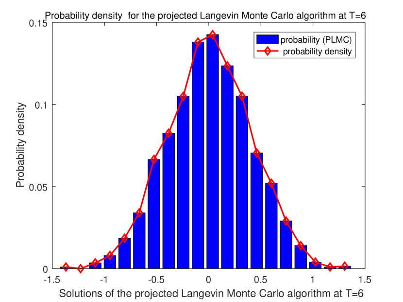
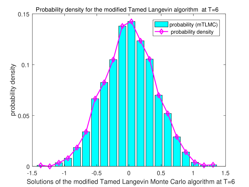
Figure 1: Probability density of the first component of the double-well model.

Convergence test. Moving on to the convergence analysis, we run the PLMC algorithm (2.17) for the Langevin SDEs with drift (6.1) by different stepsizes and dimension $d\in\{6,10,50,100\}$ till $T=6$. Further, the exact solutions are represented by the MTLMC algorithm (6.4) at a fine stepsize $h_{ref}=2^{-13}$. The reference lines of slope $0.5$ and $1$ are presented as well. From Figure 2, Figure 3, Figure 4 and Figure 5, it is natural to obtain that the convergence rate under the total variation distance with $d\in\{6,10,50,100\}$ is of order $1$. Also, all weak errors are reported in Table 1, Table 2, Table 3 and Table 4.

Weak errors for $d=6$
$h$\$\phi$	$\phi_{1}(x)$	$\exp(-\|x\|)$	$\phi_{2}(x)$	$\arctan(\|x\|)$
$2^{-5}$	3.13e-02	8.64e-04	3.83e-02	1.25e-03
$2^{-6}$	1.33e-02	5.36e-04	1.68e-02	7.63e-04
$2^{-7}$	6.00e-03	1.95e-04	8.00e-03	2.81e-04
$2^{-8}$	3.00e-03	1.14e-04	4.12e-03	1.63e-04
$2^{-9}$	1.33e-03	5.19e-05	1.83e-03	7.39e-05

Table 1: Weak errors of PLMC algorithm for the double well model ($d=6$)

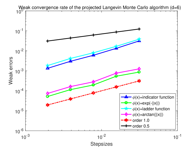
Figure 2: Weak convergence rates of PLMC algorithm for the double well model ($d=6$)

Weak errors for $d=10$
$h$\$\phi$	$\phi_{1}(x)$	$\exp(-\|x\|)$	$\phi_{2}(x)$	$\arctan(\|x\|)$
$2^{-5}$	6.13e-02	3.95e-03	8.52e-02	5.51e-03
$2^{-6}$	2.67e-02	1.93e-03	3.63e-02	2.68e-03
$2^{-7}$	1.50e-02	9.50e-04	2.10e-03	1.32e-03
$2^{-8}$	6.00e-03	4.64e-04	8.50e-03	6.43e-04
$2^{-9}$	2.33e-03	2.00e-04	3.67e-03	2.78e-04

Table 2: Weak errors of PLMC algorithm for the double well model ($d=10$)

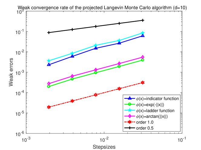
Figure 3: Weak convergence rates of PLMC algorithm for the double well model ($d=10$)

Weak errors for $d=50$
$h$\$\phi$	$\phi_{1}(x)$	$\exp(-\|x\|)$	$\phi_{2}(x)$	$\arctan(\|x\|)$
$2^{-5}$	3.14e-01	1.70e-02	4.01e-01	2.53e-02
$2^{-6}$	1.59e-01	6.88e-03	1.99e-01	1.02e-02
$2^{-7}$	7.17e-02	3.17e-03	8.97e-02	4.67e-03
$2^{-8}$	2.70e-02	1.41e-03	3.38e-02	2.08e-03
$2^{-9}$	1.20e-02	5.62e-04	1.50e-02	8.26e-04

Table 3: Weak errors of PLMC algorithm for the double well model ($d=50$)

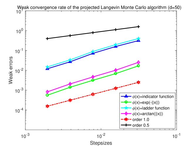
Figure 4: Weak convergence rates of PLMC algorithm for the double well model ($d=50$)

Weak errors for $d=100$
$h$\$\phi$	$\phi_{1}(x)$	$\exp(-\|x\|)$	$\phi_{2}(x)$	$\arctan(\|x\|)$
$2^{-5}$	5.87e-01	2.64e-02	4.45e-01	4.36e-02
$2^{-6}$	1.52e-01	9.34e-03	1.12e-02	1.50e-02
$2^{-7}$	3.67e-02	3.93e-03	2.63e-02	6.27e-03
$2^{-8}$	1.30e-02	1.65e-03	9.25e-03	2.63e-03
$2^{-9}$	5.67e-03	5.32e-04	4.08e-03	8.46e-04

Table 4: Weak errors of PLMC algorithm for the double well model ($d=100$)

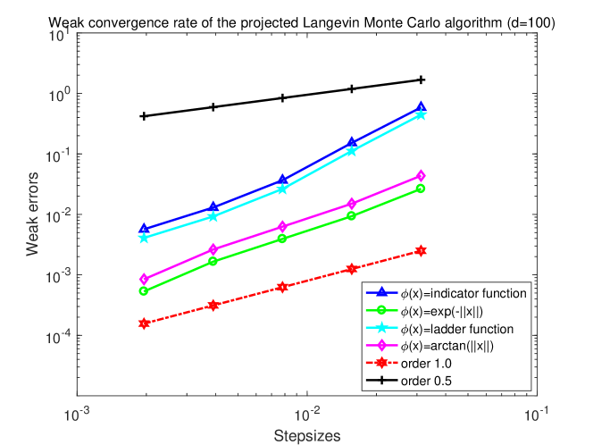
Figure 5: Weak convergence rates of PLMC algorithm for the double well model ($d=100$)

Appendix A Proof of Lemmas in Section 3

A.1 Proof of Lemma 3.1

Proof of Lemma 3.1.

Applying the Itô formula to $e^{cpt}(\epsilon_{3}+\|X_{t}\|^{2})^{p}$, for some constants $c\in(0,a_{1})$ and $\epsilon_{3}>0$, with the Cauchy-Schwarz inequality shows,

$$e^{cpt}\left(\epsilon_{3}+\|X_{t}\|^{2}\right)^{p}$$ (A.1)

$$\leq(\epsilon_{3}+\|x_{0}\|^{2})^{p}+cp\int_{0}^{t}e^{cps}\left(\epsilon_{3}+\|X_{s}\|^{2}\right)^{p}\text{d}s+2p\int_{0}^{t}e^{cps}\left(\epsilon_{3}+\|X_{s}\|^{2}\right)^{p-1}\left\langle X_{s},f(X_{s})\right\rangle\text{d}s$$

$$\quad+2\sqrt{2}p\int_{0}^{t}e^{cps}\left(\epsilon_{3}+\|X_{s}\|^{2}\right)^{p-1}\text{d}W_{s}+2p(2p-1)d\int_{0}^{t}e^{cps}\left(\epsilon_{3}+\|X_{s}\|^{2}\right)^{p-1}\text{d}s.$$

For $\gamma>1$, taking expectations on the both sides of (A.1) with Assumption 2.4 and letting $\epsilon_{3}\rightarrow 0^{+}$ yield

$$e^{cpt}\mathbb{E}\left[\|X_{t}\|^{2p}\right]$$ (A.2)

$$\leq\mathbb{E}\left[\|x_{0}\|^{2p}\right]+p\mathbb{E}\left[\int_{0}^{t}e^{cps}\Big{[}-a_{1}\|X_{s}\|^{2p+\gamma-1}+c\|X_{s}\|^{2p}+(4pd-2d+a_{2})\|X_{s}\|^{2p-2}\Big{]}\text{d}s\right].$$

Using the Young inequality

$$ab^{2p-2}\leq\dfrac{1}{p}a^{p}+\dfrac{p-1}{p}b^{2p},$$ (A.3)

for any $a,b>0$ and $p\geq 1$ suggests

$$(4pd-2d+a_{2})\|X_{s}\|^{2p-2}\leq\dfrac{(4pd-2d+a_{2})^{p}}{p}+\dfrac{p-1}{p}\|X_{s}\|^{2p}.$$ (A.4)

Putting (A.4) into (A.2) with the fact that

$$-a_{1}\|x\|^{2p+\gamma-1}+\left(c+\dfrac{p-1}{p}\right)\|x\|^{2p}\leq C,\quad\forall x\in\mathbb{R}^{d},\ p\geq 1,$$ (A.5)

where $C$ depends on $a_{1},p,\gamma$, we deduce,

$$e^{cpt}\mathbb{E}\left[\|X_{t}\|^{2p}\right]\leq\mathbb{E}\left[\|x_{0}\|^{2p}\right]+Cd^{p}\int_{0}^{t}e^{cps},$$ (A.6)

leading to

$$\mathbb{E}\left[\|X_{t}\|^{2p}\right]\leq e^{-cpt}\mathbb{E}\left[\|x_{0}\|^{2p}\right]+Cd^{p}.$$ (A.7)

Especially, for the case $\gamma=1$, recalling Assumption 2.4 and the Itô formula, we obtain

$$e^{cpt}\mathbb{E}\left[\|X_{t}\|^{2p}\right]$$ (A.8)

$$\leq\mathbb{E}\left[\|x_{0}\|^{2p}\right]+p\mathbb{E}\left[\int_{0}^{t}e^{cps}\Big{[}\big{(}-a_{1}+c\big{)}\|X_{s}\|^{2p}+\big{(}4pd-2d+a_{2}\big{)}\|X_{s}\|^{2p-2}\Big{]}\text{d}s\right].$$

Choosing $c\in(0,a_{1})$, we obtain that the following estimate holds true by the similar approach above,

$$\left(-a_{1}+c\right)\|X_{s}\|^{2p}+\big{(}4pd-2d+a_{2}\big{)}\|X_{s}\|^{2p-2}\leq Cd^{p}.$$ (A.9)

Hence, we arrive at

$$e^{cpt}\mathbb{E}\left[\|X_{t}\|^{2p}\right]\leq\mathbb{E}\left[\|x_{0}\|^{2p}\right]+Cd^{p}\int_{0}^{t}e^{cs}\text{d}s,$$ (A.10)

resulting in

$$\mathbb{E}\left[\|X_{t}\|^{2p}\right]\leq e^{-cpt}\mathbb{E}\left[\|x_{0}\|^{2p}\right]+Cd^{p}.$$ (A.11)

The proof is completed. ∎

Appendix B Proof of lemmas in Section 4

B.1 Proof of Lemma 4.2

Proof of Lemma 4.2.

The existence and the uniqueness of the mean-square derivatives up to the second order can be derived owing to Remark 2.3 (see [5, 28]). For simplicity, we denote that

$$\eta^{v_{1}}(t,x):=\mathcal{D}X^{x}_{t}v_{1},\quad\xi^{v_{1},v_{2}}(t,x):=\mathcal{D}^{2}X^{x}_{t}(v_{1},v_{2}),\quad\forall x,v_{1},v_{2}\in\mathbb{R}^{d}.$$ (B.1)

Part I: estimate of the first variation process

It follows from Remark 2.3 that,

$$\langle Df(x)y,y\rangle\leq L\|y\|^{2},\quad\forall x,y\in\mathbb{R}^{d}.$$ (B.2)

Moreover, for the first variation process of SDE (1.2), one gets

$$\text{d}\eta^{v_{1}}(t,x)=Df(X^{x}_{t})\eta^{v_{1}}(t,x)\,\text{d}t,\quad\eta^{v_{1}}(0)=v_{1}.$$ (B.3)

Taking the temporal derivative of $\|\eta^{v_{1}}(t,x)\|^{2}$, we obtain that

$$\text{d}\|\eta^{v_{1}}(t,x)\|^{2} =2\left\langle\eta^{v_{1}}(t,x),Df(X^{x}_{t})\eta^{v_{1}}(t,x)\right\rangle\leq 2L\|\eta^{v_{1}}(t,x)\|^{2},$$ (B.4)

which leads to

$$\|\eta^{v_{1}}(t,x)\|^{2}\leq e^{2Lt}\|v_{1}\|^{2}.$$ (B.5)

Part II: estimate of the second variation process

Similarly, due to the variation approach, we have the second variation process with respect to SDEs (1.2) as follows,

$$\text{d}\xi^{v_{1},v_{2}}(t,x)=\Big{(}Df(X^{x}_{t})\xi^{\upsilon_{1},\upsilon_{2}}(t,x)+D^{2}f(X^{x}_{t})\big{(}\eta^{\upsilon_{1}}(t,x),\eta^{\upsilon_{2}}(t,x)\big{)}\Big{)}\text{d}t,\quad\xi^{\upsilon_{1},\upsilon_{2}}(0)=0.$$ (B.6)

Following the same argument as before and the Young inequality, we deduce that

$$\text{d}\|\xi^{\upsilon_{1},\upsilon_{2}}(t,x)\|^{2}$$ (B.7)

$$=\Big{(}2\left\langle\xi^{\upsilon_{1},\upsilon_{2}}(t,x),Df(X^{x}_{t})\xi^{\upsilon_{1},\upsilon_{2}}(t,x)\right\rangle+2\left\langle\xi^{\upsilon_{1},\upsilon_{2}}(t,x),D^{2}f(X^{x}_{t})\big{(}\eta^{\upsilon_{1}}(t,x),\eta^{\upsilon_{2}}(t,x)\big{)}\right\rangle\Big{)}\text{d}t$$

$$\leq(2L+1)\|\xi^{\upsilon_{1},\upsilon_{2}}(t,x)\|^{2}\text{d}t+\left\|D^{2}f(X^{x}_{t})\big{(}\eta^{\upsilon_{1}}(t,x),\eta^{\upsilon_{2}}(t,x)\big{)}\right\|^{2}\text{d}t.$$

The key issue is to estimate $\left\|D^{2}f(X^{x}_{t})(\eta^{\upsilon_{1}}(t,x),\eta^{\upsilon_{2}}(t,x))\right\|_{L^{2}(\Omega,\mathbb{R}^{d})}$, where, by Assumption 2.1, the range of $\gamma$ deserves to be discussed carefully. If $1\leq\gamma\leq 2$, with (B.5) and the Hölder inequality in mind, we will arrive at, for some constants $\rho_{1},\rho_{2}>1$ with $1/\rho_{1}+1/\rho_{2}=1$, and some random variables $\upsilon_{1}\in L^{2\rho_{1}}(\Omega,\mathbb{R}^{d})$, $\upsilon_{2}\in L^{2\rho_{2}}(\Omega,\mathbb{R}^{d})$,

$$\left\|D^{2}f(X^{x}_{t})\big{(}\eta^{\upsilon_{1}}(t,x),\eta^{\upsilon_{2}}(t,x)\big{)}\right\|_{L^{2}(\Omega,\mathbb{R}^{d})} \leq C\big{\|}\left\|\eta^{\upsilon_{1}}(t,x)\right\|\cdot\left\|\eta^{\upsilon_{2}}(t,x)\right\|\big{\|}_{L^{2}(\Omega,\mathbb{R})}$$ (B.8)

$$\leq Ce^{2Lt}\left\|\upsilon_{1}\right\|_{L^{2\rho_{1}}(\Omega,\mathbb{R}^{d})}\left\|\upsilon_{2}\right\|_{L^{2\rho_{2}}(\Omega,\mathbb{R}^{d})}.$$

Taking this into (B.7) shows

$$\mathbb{E}\left[\|\xi^{\upsilon_{1},\upsilon_{2}}(t,x)\|^{2}\right]\leq(2L+1)\int_{0}^{t}\mathbb{E}\left[\|\xi^{\upsilon_{1},\upsilon_{2}}(s,x)\|^{2}\right]\text{d}s+C\int_{0}^{t}e^{4Ls}\text{d}s\left\|\upsilon_{1}\right\|^{2}_{L^{2\rho_{1}}(\Omega,\mathbb{R}^{d})}\left\|\upsilon_{2}\right\|^{2}_{L^{2\rho_{2}}(\Omega,\mathbb{R}^{d})},$$ (B.9)

and by the Gronwall inequality we get the result. If $\gamma>2$, using the Hölder inequality with (B.5) yields, for $\rho_{1},\rho_{2},\rho_{3}>1$ with $1/\rho_{1}+1/\rho_{2}+1/\rho_{3}=1$,

$$\left\|D^{2}f(X^{x}_{t})\big{(}\eta^{\upsilon_{1}}(t,x),\eta^{\upsilon_{2}}(t,x)\big{)}\right\|_{L^{2}(\Omega,\mathbb{R}^{d})}$$ (B.10)

$$\leq C\big{\|}\left(1+\|X^{x}_{t}\|\right)^{\gamma-2}\left\|\eta^{\upsilon_{1}}(t,x)\right\|\cdot\left\|\eta^{\upsilon_{2}}(t,x)\right\|\big{\|}_{L^{2}(\Omega,\mathbb{R})}$$

$$\leq C\big{\|}\left(1+\|X^{x}_{t}\|\right)^{\gamma-2}\big{\|}_{L^{2\rho_{1}}(\Omega,\mathbb{R})}\left\|\eta^{\upsilon_{1}}(t,x)\right\|_{L^{2\rho_{2}}(\Omega,\mathbb{R}^{d})}\left\|\eta^{\upsilon_{2}}(t,x)\right\|_{L^{2\rho_{3}}(\Omega,\mathbb{R}^{d})}.$$

In the same manner, thanks to the Gronwall inequality, we have, for some random variables $\upsilon_{1}\in L^{2\rho_{2}}(\Omega,\mathbb{R}^{d})$ and $\upsilon_{2}\in L^{2\rho_{3}}(\Omega,\mathbb{R}^{d})$,

$$\|\xi^{\upsilon_{1},\upsilon_{2}}(t,x)\|_{L^{2}(\Omega,\mathbb{R}^{d})}\leq Ce^{(3L+1/2)t}\sup_{r\in[0,\infty)}\left\|\left(1+\|X^{x}_{r}\|\right)^{\gamma-2}\right\|_{L^{2\rho_{1}}(\Omega,\mathbb{R})}\left\|\upsilon_{1}\right\|_{L^{2\rho_{2}}(\Omega,\mathbb{R}^{d})}\left\|\upsilon_{2}\right\|_{L^{2\rho_{3}}(\Omega,\mathbb{R}^{d})}.$$ (B.11)

Combining (B.9) and (B.11), the proof is completed. ∎

Appendix C Proof of Lemmas in Section 5

C.1 Proof of Lemma 5.2

Proof of Lemma 5.2.

Consider these two measurable sets

$$\mathcal{A}_{h}:=\left\{\omega\in\Omega:\|\zeta(\omega)\|\leq\vartheta d^{\frac{1}{2\gamma}}h^{-\frac{1}{2\gamma}}\right\},\quad\mathcal{A}_{h}^{c}:=\Omega\backslash\mathcal{A}_{h}.$$ (C.1)

Therefore, owing to the Hölder inequality, for $1/q+1/q^{\prime}=1$, we obtain

$$\mathbb{E}\left[\|\zeta-\mathscr{P}(\zeta)\|\right]=\mathbb{E}\left[\|\zeta-\mathscr{P}(\zeta)\|\textbf{1}_{\mathcal{A}_{h}^{c}}\right]\leq\|\zeta-\mathscr{P}(\zeta)\|_{L^{q}(\Omega,\mathbb{R}^{d})}\|\textbf{1}_{\mathcal{A}_{h}^{c}}\|_{L^{q^{\prime}}(\Omega,\mathbb{R})}.$$ (C.2)

Here, using Lemma 3.3 with the triangular inequality yields

$$\|\zeta-\mathscr{P}(\zeta)\|_{L^{q}(\Omega,\mathbb{R}^{d})}\leq\|\zeta\|_{L^{q}(\Omega,\mathbb{R}^{d})}+\|\mathscr{P}(\zeta)\|_{L^{q}(\Omega,\mathbb{R}^{d})}\leq 2\|\zeta\|_{L^{q}(\Omega,\mathbb{R}^{d})}.$$ (C.3)

In addition, it follows from the Markov inequality that,

$$\|\textbf{1}_{\mathcal{A}_{h}^{c}}\|_{L^{q^{\prime}}(\Omega,\mathbb{R})}=\big{(}\mathbb{P}(\mathcal{A}_{h}^{c})\big{)}^{\frac{1}{q^{\prime}}}\leq\vartheta^{-\frac{\beta}{q^{\prime}}}d^{-\frac{\beta}{2\gamma q^{\prime}}}h^{\frac{\beta}{2\gamma q^{\prime}}}\|\zeta\|^{\frac{\beta}{q^{\prime}}}_{L^{\beta}(\Omega,\mathbb{R}^{d})}.$$ (C.4)

We choose $q=4\gamma+1$, $q^{\prime}=1+1/4\gamma$ and $\beta=4\gamma+1$, then the proof is completed.

∎

Appendix D Proof of Remark 2.8

Proof.

Given tolerance $\epsilon\in(0,1)$ and $k\in\mathbb{N}$, it follows from Theorem 2.6 that

$$\left\|\Pi(\widetilde{Y}^{x_{0}}_{k})-\pi\right\|_{\text{TV}}\leq\underbrace{Ce^{-Ckh}\left(1+\mathbb{E}\left[\|x_{0}\|^{2}\right]\right)}_{\leq\frac{\epsilon}{2}}+\underbrace{Cd^{3/2}h|\ln h|}_{\leq\frac{\epsilon}{2}}.$$ (D.1)

Solving the first part on the right hand of (D.1) yields

$$k\geq\dfrac{C}{h}\ln\big{(}\dfrac{1}{\epsilon}\big{)}.$$ (D.2)

The second part on the right hand of (D.1) goes to

$$\dfrac{\tfrac{1}{h}}{\ln(\tfrac{1}{h})}\geq C\dfrac{d^{3/2}}{\epsilon},$$ (D.3)

leading to

$$\dfrac{1}{h}\geq C\dfrac{d^{3/2}}{\epsilon}\cdot\ln\big{(}\dfrac{d}{\epsilon}\big{)}.$$ (D.4)

To obtain this result, from (D.3), we denote by $\widehat{C}:=Cd^{3/2}/\epsilon$ to find an appropriate $1/h$ such that

$$\dfrac{1}{h}-\widehat{C}\ln\big{(}\dfrac{1}{h}\big{)}\geq 0.$$ (D.5)

As we know, the function $x-\widehat{C}\ln x$ is increasing when $x\geq\widehat{C}$. Hence one can take $1/h=\mathcal{O}(\widehat{C}\ln\widehat{C})$, for example, choosing $1/h=2\widehat{C}\ln\widehat{C}$, to make (D.4) hold. Plugging this into (D.2) yields

$$k\geq C\dfrac{d^{3/2}}{\epsilon}\cdot\ln\big{(}\dfrac{d}{\epsilon}\big{)}\cdot\ln\big{(}\dfrac{1}{\epsilon}\big{)},$$ (D.6)

which completes the proof. ∎

References

- [1] W.-J. Beyn, E. Isaak, and R. Kruse. Stochastic C-stability and B-consistency of explicit and implicit Euler-type schemes. Journal of Scientific Computing, 67(3):955–987, 2016.
- [2] W.-J. Beyn, E. Isaak, and R. Kruse. Stochastic C-stability and B-consistency of explicit and implicit Milstein-type schemes. Journal of Scientific Computing, 70(3):1042–1077, 2017.
- [3] C.-E. Bréhier. Approximation of the invariant measure with an Euler scheme for stochastic PDEs driven by space-time white noise. Potential Analysis, 40(1):1–40, 2014.
- [4] N. Brosse, A. Durmus, É. Moulines, and S. Sabanis. The tamed unadjusted Langevin algorithm. Stochastic Processes and their Applications, 129(10):3638–3663, 2019.
- [5] S. Cerrai. Second order PDE’s in finite and infinite dimension: a probabilistic approach. Springer, 2001.
- [6] X. Cheng, N. S. Chatterji, Y. Abbasi-Yadkori, P. L. Bartlett, and M. I. Jordan. Sharp convergence rates for Langevin dynamics in the nonconvex setting. arXiv preprint arXiv:1805.01648, 2018.
- [7] G. Da Prato. An introduction to infinite-dimensional analysis. Springer Science & Business Media, 2006.
- [8] A. S. Dalalyan. Theoretical guarantees for approximate sampling from smooth and log-concave densities. Journal of the Royal Statistical Society Series B: Statistical Methodology, 79(3):651–676, 2017.
- [9] A. Durmus and É. Moulines. Nonasymptotic convergence analysis for the unadjusted Langevin algorithm. The Annals of Applied Probability, 27(3):1551–1587, 2017.
- [10] A. Durmus and É. Moulines. High-dimensional Bayesian inference via the unadjusted Langevin algorithm. Bernoulli, 25(4A):2854–2882, 2019.
- [11] K. D. Elworthy and X.-M. Li. Formulae for the derivatives of heat semigroups. Journal of Functional Analysis, 125(1):252–286, 1994.
- [12] B. Goldys. Exponential Ergodicity for Stochastic Reaction–Diffusion Equations. Stochastic Partial Differential Equations and Applications-VII, page 115, 2005.
- [13] M. Hutzenthaler, A. Jentzen, and P. E. Kloeden. Strong and weak divergence in finite time of Euler’s method for stochastic differential equations with non-globally Lipschitz continuous coefficients. Proceedings of the Royal Society A: Mathematical, Physical and Engineering Sciences, 467(2130):1563–1576, 2011.
- [14] M. Hutzenthaler, A. Jentzen, and P. E. Kloeden. Strong convergence of an explicit numerical method for SDEs with nonglobally Lipschitz continuous coefficients. The Annals of Applied Probability, 22(4):1611–1641, 2012.
- [15] R. Li, H. Zha, and M. Tao. Sqrt (d) Dimension Dependence of Langevin Monte Carlo. In The International Conference on Learning Representations, 2022.
- [16] X. Li, X. Mao, and G. Yin. Explicit numerical approximations for stochastic differential equations in finite and infinite horizons: truncation methods, convergence in pth moment and stability. IMA Journal of Numerical Analysis, 39(2):847–892, 2019.
- [17] X. Li, F.-Y. Wang, and L. Xu. Unadjusted Langevin Algorithms for SDEs with Hölder Drift. arXiv preprint arXiv:2310.00232, 2023.
- [18] M. B. Majka, A. Mijatović, and L. Szpruch. Nonasymptotic bounds for sampling algorithms without log-concavity. The Annals of Applied Probability, 30(4):1534–1581, 2020.
- [19] J. C. Mattingly, A. M. Stuart, and D. J. Higham. Ergodicity for SDEs and approximations: locally Lipschitz vector fields and degenerate noise. Stochastic processes and their applications, 101(2):185–232, 2002.
- [20] A. Neufeld, M. N. C. En, and Y. Zhang. Non-asymptotic convergence bounds for modified tamed unadjusted Langevin algorithm in non-convex setting. arXiv preprint arXiv:2207.02600, 2022.
- [21] G. Pages and F. Panloup. Unadjusted Langevin algorithm with multiplicative noise: Total variation and Wasserstein bounds. The Annals of Applied Probability, 33(1):726–779, 2023.
- [22] C. Pang, X. Wang, and Y. Wu. Linear implicit approximations of invariant measures of semi-linear SDEs with non-globally Lipschitz coefficients. arXiv preprint arXiv:2308.12886, 2023.
- [23] S. Sabanis. Euler approximations with varying coefficients: the case of superlinearly growing diffusion coefficients. The Annals of Applied Probability, 26(4):2083–2105, 2016.
- [24] Ł. Szpruch and X. Zhāng. V-integrability, asymptotic stability and comparison property of explicit numerical schemes for non-linear SDEs. Mathematics of Computation, 87(310):755–783, 2018.
- [25] X. Wang and S. Gan. The tamed Milstein method for commutative stochastic differential equations with non-globally Lipschitz continuous coefficients. Journal of Difference Equations and Applications, 19(3):466–490, 2013.
- [26] X. Wang, J. Wu, and B. Dong. Mean-square convergence rates of stochastic theta methods for SDEs under a coupled monotonicity condition. BIT Numerical Mathematics, 60(3):759–790, 2020.
- [27] X. Wang, Y. Zhao, and Z. Zhang. Weak error analysis for strong approximation schemes of SDEs with super-linear coefficients. IMA Journal of Numerical Analysis, page drad083, 11 2023.
- [28] Y. Zhao, X. Wang, and Z. Zhang. Second-order numerical methods of weak convergence for SDEs with super-linear coefficients. preprint, 2023.