High-order Finite-Volume Central Targeted ENO Family Scheme for Compressible Flows in Unstructured Meshes

Abstract

Due to its innovative weighting method, the high-order target ENO (TENO) system has shown tremendous potential for complicated flow prediction. For unstructured meshes, we have developed non-oscillatory central target ENO family schemes in this study. In comparison with standard WENO schemes, the compact directional stencils significantly enhance the possibility that one of them will be in smooth area. The scheme is inherently limited in size in order to simplify the directional stencils in implementation. Following an effective scale separation method, we employ the ENO-like stencil selection technique, which selects candidate reconstructions from large central stencils in smooth areas to enforce the ENO property and from small directional stencils at discontinuities to restore high-order accuracy. With the validation of a number of test cases, a detailed comparison of CWENO, TENO, CTENO and CTENOZ schemes was carried out to assess their performance based on accuracy, robustness, parallel scalability and run time. Our findings demonstrate high-order precision, lower numerical dissipation, and superior sharp shock-capturing performance of proposed CTENO and CTENOZ schemes.

1 Introdution

In computational fluid dynamics, high-order accuracy techniques are an essential area of study. It is necessary for the solution to resolve smooth flows with high order precision while keeping the solution non-oscillatory in the presence of discontinuities. High order and low dissipation characteristics are crucial for resolving small-scale flow patterns in complicated flow simulations. These conditions provide challenges for the development of current algorithms for computation. Several methods have been put out for this target, such as artificial viscosity schemes[1], total variation diminishing (TVD) schemes[2], essentially non-oscillatory (ENO) schemes[3] and weighted essentially non-oscillatory (WENO) schemes[4].

WENO schemes, considered as most efficient high-order numerical methods for shock-capturing, were initially proposed in finite-volume format by Liu et al. [4] and subsequently expanded to finite-difference format by Jiang and Shu et al.[5]. These schemes were derived from ENO proposed by Harten et al.[3] and surpass ENO by incorporating all candidate stencils using indicators of smoothness. This guarantees restoration of globally achieving optimal high-order accuracy in smooth areas asymptotically. Subsequently, WENO scheme near critical points was improved by redefining the nonlinear weights, leading to low dissipation such as WENO-M[6] and WENO-Z[7]. However, this practical use of WENO family schemes in accurately predicting complex flows has shown that they introduce excessive dissipation when used for under-resolved simulations, such as turbulence [8]. To enhance the low dissipation characteristic of WENO schemes, several approaches have been explored. These include increasing the non-smooth weights of stencil points [9], limiting nonlinear adjustments in smooth areas [10], optimizing spectral characteristics of linear scheme background [11], and new nonlinear weights for improving accuracy and resolution[12]. For more comprehensive examination of WENO and their respective details, readers are advised to refer [13].

Fu et al.[14, 15] recently explored a group of schemes, known as targeted ENO (TENO). Utilizing ENO-like stencil selection methods, TENO possess low dissipation while still preserving the ability to capture sharp shocks. A notable feature of TENO schemes is their capability to maintain the exact linear scheme for intermediate wavenumbers, without compromising their ability to capture strong discontinuities. TENO schemes on structured meshes have found applications in various flow scenarios[16], such as multi-phase flows[17], detonation simulations[18], and turbulent flows[19, 20]. While TENO schemes have been successful in demonstrating their effectiveness for compressible fluid and predicting turbulence on structured grids, extending their applicability to unstructured meshes presents a significant challenge. Simultaneously achieving accuracy with high-order in smooth areas, small structure features with lower dissipation and precise shock-capturing abilities, ensuring numerical stability further compounds the difficulty.

When it comes to handling intricate geometries, it becomes crucial to extend high order schemes to unstructured meshes[21]. As evidenced in [22, 23], when utilizing the traditional WENO method on unstructured grids, like triangular or tetrahedral, optimal linear coefficients needed to create reconstructions with orders by collecting small stencil elements can alter considerably based on different quadrature points and mesh configurations. In certain scenarios, these weights may result in numerical instabilities and necessitate additional specific handling[24]. One possibility is to utilize multi-resolution WENO schemes[25] or adaptive order WENO schemes[26]. One potential technique to alleviate the hardship of defining the ideal linear weights is to lower desired order of accuracy for large stencils to match small candidate stencils[27]. The central WENO (CWENO) schemes [28, 29], incorporate both large and small stencils, implementing customized weighting strategies that permit flexibility in choosing the linear weights. Utilization of the CWENO scheme provides benefits of decreased computational footprints compared with conventional WENO because of smaller directional stencil size. Notably, Tsoutsanis et al.[30] succeed in expanding high-order WENO to unstructured meshes with mixed-element and accurately forecasted complex turbulent flows [31] based on the strategy of weight. Recently, Ji et al.[32, 33] extended TENO to unstructured grids within the finite-volume methods, which offers to seventh order accuracy.

Unlike WENO for unstructured grids[30], CWENO schemes have received less attention despite they have increased robustness. The CWENO reduce width of directional stencils, resulting in more likelihood of one stencil existing in smooth region. This enhanced robustness sets it apart from WENO schemes[29]. In this research, our aim is to develop central target ENO (CTENO) and CTENOZ scheme on unstructured grids under finite volume framework with high-order. Compact design of CTENO scheme makes it particularly well-suited for complex flow simulation. In order to achieve reduced dissipation and improved shock-capture abilities, we utilize stencil selection strategy inspired by ENO method[32], which is built upon a customized arrangement of candidate stencils, comprising of larger and multiple smaller stencils. The CWENO and CTENO schemes have incorporated central stencil algorithm with stencil-based compact (SBC) and directional stencil Type 3 algorithm[34], resulting a significant reduction in their computational footprint. The construction of directional stencils included in central stencil is relatively simple and compact (especially for higher-order cases). This simplifies the process compared with original WENO. We have developed the CTENO scheme with a spatial accuracy of up to 7th order for unstructured meshes. Following the WENOZ and CWENOZ scheme[7, 30], the CTENOZ scheme is provided to decrease the numerical dissipation based on CTENO scheme. Our ultimate aim focus on enhancing affordability and robustness of this class of schemes, even in large-scale industrial applications.

This proposed CTENO and CTENOZ scheme is implemented in UCNS3D open source solver[35]. Our main focus is to assess its performance in accuracy, robustness, parallel scalability and run time for various test benchmarks[36, 37, 38, 39, 40]. Additionally, we compare the numerical results obtained from CTENO and CTENOZ schemes with TENO and CWENO schemes. The paper is structured as follows: Section 2 introduces numerical framework used to finite-volume methodology with high-order on unstructured grids, including process of reconstruction for WENO, CWENO, TENO, CTENO and CTENOZ, as well as the selected fluxes and temporal discretization methods. In Section 3, we present the results obtained from test benchmarks and compare them with analytical, reference, or experimental solutions. Finally, Section 4 concludes research.

2 Numerical framework

In this study, we examine the Euler equation, which is commonly known as hyperbolic conservation laws. The conservative form of these equations is expressed by

$$\frac{\partial U}{\partial t}+\bigtriangledown\cdot(F(U))=0,$$ (1)

where $U=U(x,y,z,t)$ is vector of conserved variables, $F(U)=(F^{x}(U),F^{y}(U),F^{z}(U))$ is convection flux functions. The physical domain comprises a mix of hexahedral,tetrahedral, prism, or pyramid elements in 3D, as well as triangular or quadrilateral elements in 2D. Integrating Equation 1 in considered element $i$ presents in the following format.

$$\frac{\mathrm{d}U_{i}}{\mathrm{d}t}=-\frac{1}{\mid V_{i}\mid}\sum_{j}^{N_{f}}\sum_{k}^{N_{q}}F^{n_{i,j}}(U_{i,j,L}^{n}(x_{i,j,k},t),U_{i,j,R}^{n}(x_{i,j,k},t))\omega_{k}\mid A_{i,j}\mid,$$ (2)

where $U_{i}=\frac{1}{\mid V_{i}\mid}\int_{V_{i}}U(x,y,z)dV$ is the cell average value of conserved variables, $V_{i}$ is volume of considered element $i$, and $F^{n_{i,j}}$ is numerical flux function in normal direction of interface between cell $i$ and its adjacent cell $j$. $N_{f}$ is total number of cell faces, $N_{q}$ are quadrature points utilized to approximate surface integrals of high-order. $U_{i,j,L}^{n}$ and $U_{i,j,R}^{n}$ are the approximate solutions on the interface from the left and right, respectively. To approximate volume/surface/line integrals, Gauss quadrature rule is employed, which suits the polynomial order effectively. $\omega_{k}$ is weight assigned to Gauss integration point $x_{i,j,k}$, and$\mid A_{i,j}\mid$ is surface area of face $j$. Temporal discretization method employed is the 4th-order explicit Runge-Kutta method[41], unless stated otherwise.

2.1 Reconstruction

For considered element $i$, $r$ order polynomial $p_{i}(x,y,z)$ can provides $r+1$ order of accuracy, by maintaining that possess an equivalent mean value with $U_{i}$, which is expressed as:

$$U_{i}=\frac{1}{\mid V_{i}\mid}\int_{V_{i}}U(x,y,z)dV=\frac{1}{\mid V_{i}\mid}\int_{V_{i}}P_{i}(x,y,z)dV.$$ (3)

For unstructured grids comprising cells of diverse form, converting cells from the physical space $(x,y,z)$ to a reference space $(\xi,\eta,\zeta)$ to mitigate scaling effects is advantageous, while ensuring the spatial cell average of conserved variable remains unchanged during the transformation.

$$U_{i}=\frac{1}{\mid V_{i}\mid}\int_{V_{i}}U(x,y,z)dV=\frac{1}{\mid V_{i}^{{}^{\prime}}\mid}\int_{V_{i}^{{}^{\prime}}}U(\xi,\eta,\zeta)d\xi d\eta d\zeta.$$ (4)

To compute reconstructed values of specified cell $i$, compact stencil $S$ consisting of $M+1$ elements including the targeted element $i$, is created alongside adjacent elements of $i$. SBC is utilized because of lower computational cost and improved robustness, for more details please refer to [34]. We employ $M=2K$ for improved robustness as mentioned in various previous studies [34, 42], where $K$ is number of coefficients in a polynomial:

$$K(r,d)=\frac{1}{d!}\prod_{l=1}^{d}(r+l),$$ (5)

where $d\in[2,3]$ is space dimensions. This entire stencil is converted to reference space $S^{{}^{\prime}}$. The $r_{th}$ order reconstructed polynomials are extended by a set of polynomial basis functions $\phi_{k}(\xi,\eta,\zeta)$:

$$p(\xi,\eta,\zeta)=\sum_{k=0}^{K}a_{k}\phi_{k}(\xi,\eta,\zeta)=U_{0}+\sum_{k=1}^{K}a_{k}\phi_{k}(\xi,\eta,\zeta),$$ (6)

where $U_{0}$ demonstrates cell average solution in specified cell $i$, $a_{k}$ denotes the degrees of freedom. To guarantee the limitation of Equation 3 for the element $i$ and satisfy choices of all the elements in the stencil, the basis functions are expressed as

$$\phi_{k}(\xi,\eta,\zeta)=\psi_{k}(\xi,\eta,\zeta)-\frac{1}{\mid V_{0}^{{}^{\prime}}\mid\ }\int_{V_{0}^{{}^{\prime}}}\psi_{k}d\xi d\eta d\zeta\quad\psi_{k}=\xi,\eta,\zeta,\xi^{2},\eta^{2},\zeta^{2},\xi\eta,\xi\zeta,\eta\zeta...\quad k=1,2...K.$$ (7)

The degrees of freedom $a_{k}$ for cell $m$ in the stencil are defined by meeting requirement that cell average value of reconstructed polynomial $p(\xi,\eta,\zeta)$ maintain the same with the cell average value of solution $U_{m}$.

$$\int_{V_{m}^{{}^{\prime}}}p(\xi,\eta,\zeta)d\xi d\eta d\zeta=\mid V_{m}^{{}^{\prime}}\mid U_{0}+\sum_{k=1}^{K}\int_{V_{m}^{{}^{\prime}}}a_{k}\phi_{k}d\xi d\eta d\zeta=\mid V_{m}^{{}^{\prime}}\mid U_{m}\quad m=1,2...M.$$ (8)

Indicating the calculations of basis function integral $k$ of cell $m$ in stencils, the vector $A_{mk}$ and $b$ respectively is expressed as:

$$A_{mk}=\int_{V_{m}^{{}^{\prime}}}\phi_{k}d\xi d\eta d\zeta\quad b_{m}=\mid V_{m}^{{}^{\prime}}\mid(U_{m}-U_{0}).$$ (9)

The degrees of freedom in the equations can be formulated in matrix format

$$\sum_{k=1}^{K}A_{mk}a_{k}=b_{m}.$$ (10)

The matrix $A_{mk}$ exclusively includes the geometric data for each element within the considered stencil $S$. $A_{mk}$ can be simplified by employing QR decomposition method with Householder transformations [43].

$$a_{k}=(A_{mk}^{T}A_{mk})^{-1}A_{mk}^{T}b_{m}=((QR)^{T}(QR))^{-1}A_{mk}^{T}b_{m}=(R^{T}R)^{-1}A_{mk}^{T}b_{m}.$$ (11)

2.2 WENO schemes

In hyperbolic systems, high-order linear reconstruction scheme is inappropriate to handle discontinuous shockwaves. WENO scheme utilizes a combination of non-linear reconstruction polynomials obtained by central stencil and directional stencil [5]. The weight assigned to each polynomial depends on solution’s smoothness. The polynomials employed in WENO are stated as follows:

$$p_{i}(\xi,\eta,\zeta)^{WENO}=\sum_{s=1}^{s_{t}}\omega_{s}p_{s}(\xi,\eta,\zeta),$$ (12)

where $s_{t}$ is total number of stencils, nonlinear weight $w_{k}$ is given by

$$\omega_{s}=\frac{\tilde{\omega}}{\sum_{s=1}^{s_{t}}\tilde{\omega}}\quad,where\quad\tilde{\omega}=\frac{\lambda_{s}}{(\epsilon+SI_{s})^{b}}.$$ (13)

Smoothness indicator $SI_{s}$ is calculated by:

$$SI_{s}=\sum_{q=1}^{r}\int_{V_{0}^{{}^{\prime}}}(D^{q}p_{s}(\xi,\eta,\zeta))^{2}d\xi d\eta d\zeta,$$ (14)

where $r$ is the order of polynomial, $b=4$ and $D$ is derivative operator, $\epsilon=10^{-6}$ is utilized to prevent division by zero, $\lambda_{s}$ is linear weight. The central stencil is given significant large $\lambda_{1}$ and directional stencils are given $\lambda_{s}=1$. Previous subsection discussed the assembly of linear candidate stencil reconstructions, defined by $p_{s}(\xi,\eta,\zeta)$, that exhibit precise orders. These reconstructed candidates maintain criteria of matching cell average results of the relevant elements. They are obtained by employing the identical limited least-squares techniques to resolve over-determined linear systems. While the application of characteristic varibles decomposition in process substantially raises the computational footprints of schemes, numerous studies have consistently demonstrated the superior performance of WENO reconstructions in suppressing numerical oscillations when applied to characteristic variables, compared to primitive or conservative variables. This is particularly pronounced in cases featuring strong shocks and contact discontinuities, as evidenced by [5, 14].

2.3 CWENO schemes

The CWENO scheme originates from the methodology proposed by Tsoutsanis and Dumbser [30]. This approach utilizes a combination of optimal polynomial $p_{opt}$ with high-order and a set of polynomials with lower-order. The high-order polynomial is reconstructed by employing an extended central stencil that corresponds to the required polynomial order, while lower-order polynomials are reconstructed using directional stencils with compactness. All polynomials must fullfil same condition of matching the cell average values of the results, and solve with the same limited least-squares technique. In comparison to traditional WENO schemes, the CWENO scheme decreases computational expenses by employing smaller directional stencils within the central stencil (see Fig. 1). This method establishes an optimal polynomial, which is a high-order polynomial that satisfies the desired accuracy order. The optimal polynomial’s definition is provided by

$$p_{opt}=\sum_{s=1}^{s_{t}}\lambda_{s}p_{s}(\xi,\eta,\zeta),$$ (15)

where $s_{t}$ is total number of stencils, $s=1$ is central stencil, $s=(2,3,...s_{t})$ is directional stencil, and $\lambda_{s}$ is linear coefficient, whose sum equals to $1$. The $p_{1}$ obtained by deducting lower-order polynomials from optimal polynomial is given in the following manner:

$$p_{1}(\xi,\eta,\zeta)=\frac{1}{\lambda_{1}}(p_{opt}(\xi,\eta,\zeta)-\sum_{s=2}^{s_{t}}\lambda_{s}p_{s}(\xi,\eta,\zeta)).$$ (16)

The CWENO reconstructed polynomial is expressed as nonlinear combination of all polynomials by:

$$p_{i}(\xi,\eta,\zeta)^{CWENO}=\sum_{s=1}^{s_{t}}\omega_{s}p_{s}(\xi,\eta,\zeta),$$ (17)

where $\omega_{s}$ is nonlinear weight and can be calculated the same with WENO. Unlike the WENO scheme, the linear coefficients $\lambda_{s}$ are defined by

$$\lambda_{1}=1-\frac{1}{\lambda_{1}^{{}^{\prime}}}\quad and\quad\lambda_{s}=\frac{1-\lambda_{1}}{s_{t}-1},$$ (18)

where $\lambda_{1}^{{}^{\prime}}$ is an arbitrary value. When the scale of local flow is smooth, high-order reconstruction gradually approaches restoration to $p_{1}$. As discontinuities are approached, the influence of large stencil diminishes, and smooth small directional stencils take control over the polynomial of final reconstruction. Consequently, CWENO’s precision relies on reconstruction applied to large stencil, while reconstruction effectiveness of non-smooth areas is determined by small stencils.

While compactness of CWENO schemes has its benefits in regions with discontinuities on a coarse grid, the nonlinear weight of central stencil inaccurately decrease in smooth areas of the flow as a result of grid topology or morphology. As a consequence, this characteristic leads to substantial reduction in accuracy order compared with traditional WENO schemes [34]. The outcomes achieved with CWENO schemes demonstrate a greater reliance on the parameters involved, due to the need for a delicate balance and adjustment between the higher-order approximation obtained from central stencil and directional stencils.

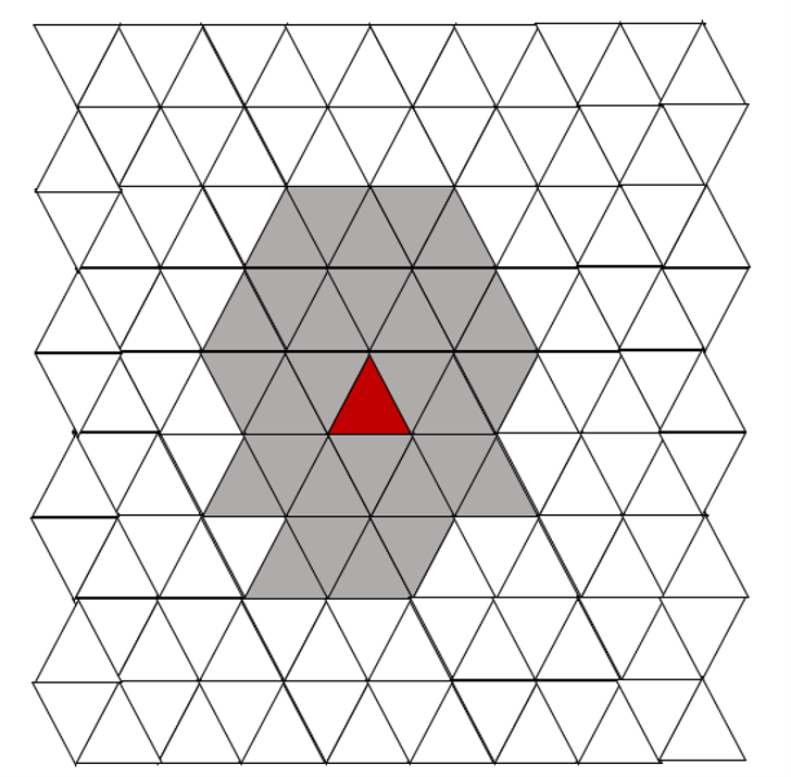
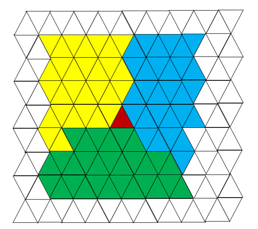
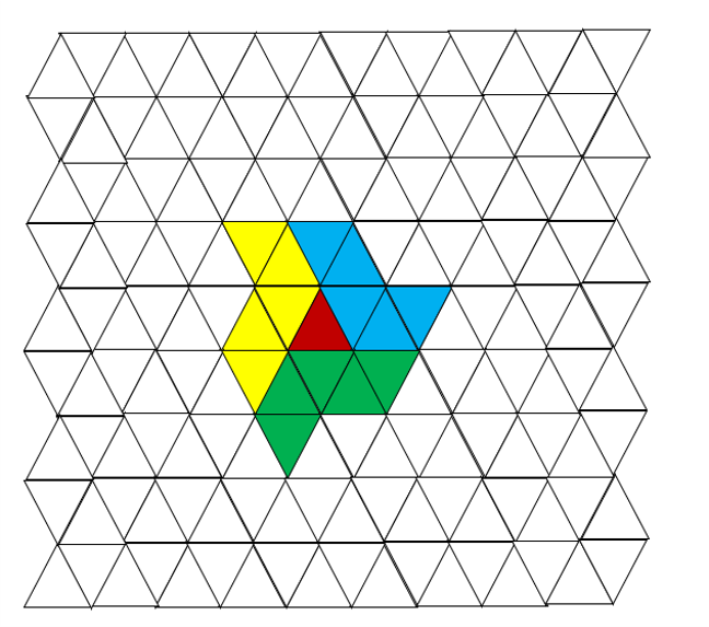
Fig. 1: The stencil for WENO on triangular grid is the fifth-order central stencil(a) and fifth-order directional stencils(b). The stencil for CWENO on triangular grid is the fifth-order central stencil(a) and second-order small directional stencils(c). The considered cell displayed in red, while the central stencil elements are displayed in gray, and each directional stencil is indicated by different colors.

2.4 TENO schemes

Similar to previous CWENO scheme, the recently proposed TENO scheme in unstructured grids aims to create stencils comprising a significant central stencil and various directional small stencils [32]. TENO schemes adopt high-order reconstruction techniques that utilizes large central stencil to resolve smooth region, while employing a serious of schemes with the small directional stencils to capture discontinuities. In order to differentiate between discontinuities and smoother scales, the TENO weighting approach utilizes a core algorithm that evaluates candidate stencils’s smoothness with noticeable separation of scale [14, 44]. This is achieved by assessing the scale separation of a stencil using the following definition.

$$\gamma_{s}=\frac{1}{(SI_{s}+\epsilon)^{6}}\quad s=1,2...s_{t}.$$ (19)

The definition of $SI_{s}$ is defined the same with WENO scheme. In comparison to WENO and CWENO schemes, for better scale separation and lower dissipation property, a larger exponent parameter is considered [5, 28]. It should be noted that previous studies using Cartesian TENO schemes [44] have shown the effectiveness of the proposed approach in achieving good scale separation. In TENO, the ENO-like method is used in stencil selection to assess each stencil as either a smooth or non-smooth candidate. To start, the indicator of measured smoothness is defined as:

$$\chi_{s}=\frac{\gamma_{s}}{\sum_{s=1}^{s_{t}}\gamma_{s}},$$ (20)

and then exposed to a rigorous truncation function,

$$\delta_{s}=\begin{cases}0,\text{ if }\chi_{s}<C_{T}\\ 1,\text{ otherwise }\end{cases}$$ (21)

where $C_{T}$ determines wavenumber and acts as a boundary between the smooth and nonsmooth scales. In practical applications, the selection of $C_{T}$ is quite flexible, ranging from $10^{-5}$ to $10^{-7}$. The proposed approach has been proven to possess numerical robustness and low-dissipation characteristics through extensive simulations performed on broad flow scales[14, 45]. In stencil selection steps, the value of parameter $C_{T}$ is set to $10^{-6}$ in order to achieve optimal performance. Further optimization related to the choice of $C_{T}$ is not covered in this paper. For more detailed information, interested readers are recommended to consult the discussions in [14, 46].

The large candidate stencil possesses the highest level of accuracy and excellent spectral properties, making it highly effective in resolving smooth flow. A collection of smaller directional stencils has been developed to capture potential discontinuities. These smaller stencils employ a non-linear adaptation technique to enhance their performance. As a result, the process of determining final reconstruction at cell interface is carried out in the following two distinct steps:

(i) Gather candidate stencils and utilize the ENO-type stencil selection method using Equation 20 and Equation 21. In the event that largest stencil is continuous, reconstruction scheme is expressed as:

$$p_{i}(\xi,\eta,\zeta)^{TENO}=p_{1}(\xi,\eta,\zeta).$$ (22)

(ii) If it is found that the largest candidate stencil is not smooth, the nonlinear adjustment between the smaller stencils will capture the discontinuities by ensuring the property and implementing the selection of ENO-type stencils. Consequently, the ultimate reconstruction scheme will be formulated by

$$p_{i}(\xi,\eta,\zeta)^{TENO}=\sum_{s=2}^{s_{t}}\omega_{s}p_{s}(\xi,\eta,\zeta),\quad where\quad\omega_{s}=\frac{\delta_{s}}{\sum_{s=2}^{s_{t}}\delta_{s}},\quad s=2,3...s_{t}.$$ (23)

2.5 CTENO schemes

Following the CWENO schemes, we utilize the optimal polynomial to calculate $p_{1}$ in Equation 15 and Equation 16. The linear coefficients $\lambda_{s}$ are defined by Equation 18. The reconstruction polynomials of CTENO schemes are as follows:

$$p_{i}(\xi,\eta,\zeta)^{CTENO}=\frac{\omega_{1}}{\lambda_{1}}(p_{opt}(\xi,\eta,\zeta)-\sum_{s=2}^{s_{t}}\lambda_{s}p_{s}(\xi,\eta,\zeta))+\sum_{s=2}^{s_{t}}\omega_{s}p_{s}(\xi,\eta,\zeta)$$ (24)

The stencil selection strategy is identical to CWENO and TENO, which contains a central stencil and a collection of directional stencils with small size. Unlike WENO and CWENO, TENO system does not calculate the non-linear coefficient $\omega_{s}$ directly. In CTENO schemes, we apply the TENO weight strategy to evaluate and capture discontinuities. The scale separation strategy of stencils is the same with that used in TENO schemes [32, 33]. After judging the smooth and non-smooth stencil with ENO-like stencil selection strategy, ultimate reconstruction are described in two steps:

(i) If large stencil is continuous, reconstruction scheme is expressed as:

$$p_{i}(\xi,\eta,\zeta)^{CTENO}=p_{1}(\xi,\eta,\zeta).$$ (25)

(ii) If large candidate stencil is non-smooth , nonlinear combination between the small candidate stencils will capture the discontinuities. Reconstruction scheme will be described by

$$p_{i}(\xi,\eta,\zeta)^{CTENO}=\sum_{s=2}^{s_{t}}\omega_{s}p_{s}(\xi,\eta,\zeta),\quad where\quad\omega_{s}=\frac{\delta_{s}}{\sum_{s=2}^{s_{t}}\delta_{s}},\quad s=2,3...s_{t}.$$ (26)

One crucial feature of CTENO is integration of optimal polynomial with high-order based on large central stencil. In smooth area, optimal polynomial is obtained to achieve the acquired accuracy level, while lower-order polynomials include smooth data at the points of discontinuous, thus reducing oscillations in calculated results. All polynomials involved in stencils are bound by the requirements as specified, matching the average value of solution in each cell. Taking into account previous version of unstructured TENO schemes [32, 33], the CTENO scheme with a high-order optimal polynomial and low-order polynomials allows for construction of unstructured CTENO reconstructions with arbitrarily high orders and exceptional numerical stability, as demonstrated in the subsequent section. For the algorithm of CTENO scheme, outlined in algorithm 1.

1 PROCEDURE CTENO scheme;

2 Compute the optimal polynomial $p_{1}$;

3 for each admissible stencil $s$ do

4       Compute the Smooth Indicator $SI_{s}$;

5      

6 end for

7!Compute Weight;

8 for each variable j do

9       $\omega_{s}=0$;

10      

11 end for

12for each admissible stencil $s$ do

13       Compute $\gamma_{s}=\frac{1}{(SI_{s}+\epsilon)^{6}}$;

14      

15 end for

16

17Computer sum $\sum_{s=1}^{s_{t}}\gamma_{s}$;

18 for each admissible stencil $s$ do

19       Compute $\chi_{s}=\frac{\gamma_{s}}{\sum_{s=1}^{s_{t}}\gamma_{s}}$;

20      

21 end for

22for each admissible stencil $s$ do

23       Compute $\delta_{s}=\begin{cases}0,&\text{ if }\chi_{s}<C_{T}\\ 1,&\text{ otherwise }\end{cases}$;

24      

25 end for

26

27if $\delta_{1}=1$ then

28       $\omega_{1}=1$;

29       for other admissible stencil $s$ do

30             $\omega_{s}=0$

31       end for

32      

33else

34       $\omega_{1}=0$;

35       for other admissible stencil $s$ do

36             $\omega_{s}=\frac{\delta_{s}}{\sum_{s=2}^{s_{t}}\delta_{s}}$

37       end for

38      

39 end if

Algorithm 1 Pseudocode for CTENO schemes computation for cell i

2.6 CTENOZ schemes

The CTENOZ essentially follows the framework of CTENO, the determinations of stencil selection strategy and optimal polynomial remains unchanged as CTENO. The primary distinction lies in the implementation of the scale separation strategy. The smoothness indicators of CWENO and CTENO schemes are obtained with polynomials from different orders. The WENOZ scheme, initially proposed by Borges et al. and Castro et al. [7, 47], is considered in the research. However, it is customized to handle polynomials with unequal orders, reconstructed stencils of varying sizes, and arbitrary shape of cells, as reported in recent studies by [48, 49]. The CTENOZ weighting strategy for scale separation aims to assess the degree of smoothness in candidate stencils by:

$$\gamma_{s}=1+\frac{\tau}{(SI_{s}+\epsilon)}\quad s=1,2...s_{t}.$$ (27)

$\tau$ is universal indicator of oscillation, which is regarded as the absolute difference values of smoothness indicators, described by:

$$\tau=(\frac{\sum_{s=2}^{s_{t}}\mid SI_{s}-SI_{1}\mid}{s_{t}-1})^{6}$$ (28)

After measuring the smoothness with strong scale-separation formula of CTENOZ schemes, the reconstruction polynomial will be calculated the same with TENO and CTENO schemes.

(i) If it is determined that central stencil is smooth, final reconstruction on the cell interface will be provided as

$$p_{i}(\xi,\eta,\zeta)^{CTENOZ}=p_{1}(\xi,\eta,\zeta).$$ (29)

(ii) Otherwise, the ultimate reconstruction scheme will be formulated by

$$p_{i}(\xi,\eta,\zeta)^{CTENOZ}=\sum_{s=2}^{s_{t}}\omega_{s}p_{s}(\xi,\eta,\zeta),\quad where\quad\omega_{s}=\frac{\delta_{s}}{\sum_{s=2}^{s_{t}}\delta_{s}},\quad s=2,3...s_{t}.$$ (30)

The algorithm of CTENOZ schemes is shown in the algorithm 2. Comparison between WENO, CWENO, TENO, CTENO, and CTENOZ schemes are shown in Fig. 2. The stencil selection, weight strategy, polynomial, linear coefficient, and scale separation for the schemes are categorized.

1 PROCEDURE CTENOZ scheme;

2 Compute the optimal polynomial $p_{1}$;

3 for each admissible stencil $s$ do

4       Compute the Smooth Indicator $SI_{s}$;

5      

6 end for

7

8Compute universal indicator of oscillation;

9 $\tau=(\frac{\sum_{s=2}^{s_{t}}\mid SI_{s}-SI_{1}\mid}{s_{t}-1})^{6}$ ;

10

11!Compute Weight;

12 for each variable j do

13       $\omega_{s}=0$;

14      

15 end for

16for each admissible stencil $s$ do

17       Compute $\gamma_{s}=1+\frac{\tau}{(SI_{s}+\epsilon)}$;

18      

19 end for

20

21Computer sum $\sum_{s=1}^{s_{t}}\gamma_{s}$;

22 for each admissible stencil $s$ do

23       Compute $\chi_{s}=\frac{\gamma_{s}}{\sum_{s=1}^{s_{t}}\gamma_{s}}$;

24      

25 end for

26for each admissible stencil $s$ do

27       Compute $\delta_{s}=\begin{cases}0,&\text{ if }\chi_{s}<C_{T}\\ 1,&\text{ otherwise }\end{cases}$;

28      

29 end for

30

31if $\delta_{1}=1$ then

32       $\omega_{1}=1$;

33       for other admissible stencil $s$ do

34             $\omega_{s}=0$

35       end for

36      

37else

38       $\omega_{1}=0$;

39       for other admissible stencil $s$ do

40             $\omega_{s}=\frac{\delta_{s}}{\sum_{s=2}^{s_{t}}\delta_{s}}$

41       end for

42      

43 end if

Algorithm 2 Pseudocode for CTENOZ schemes computation for cell i

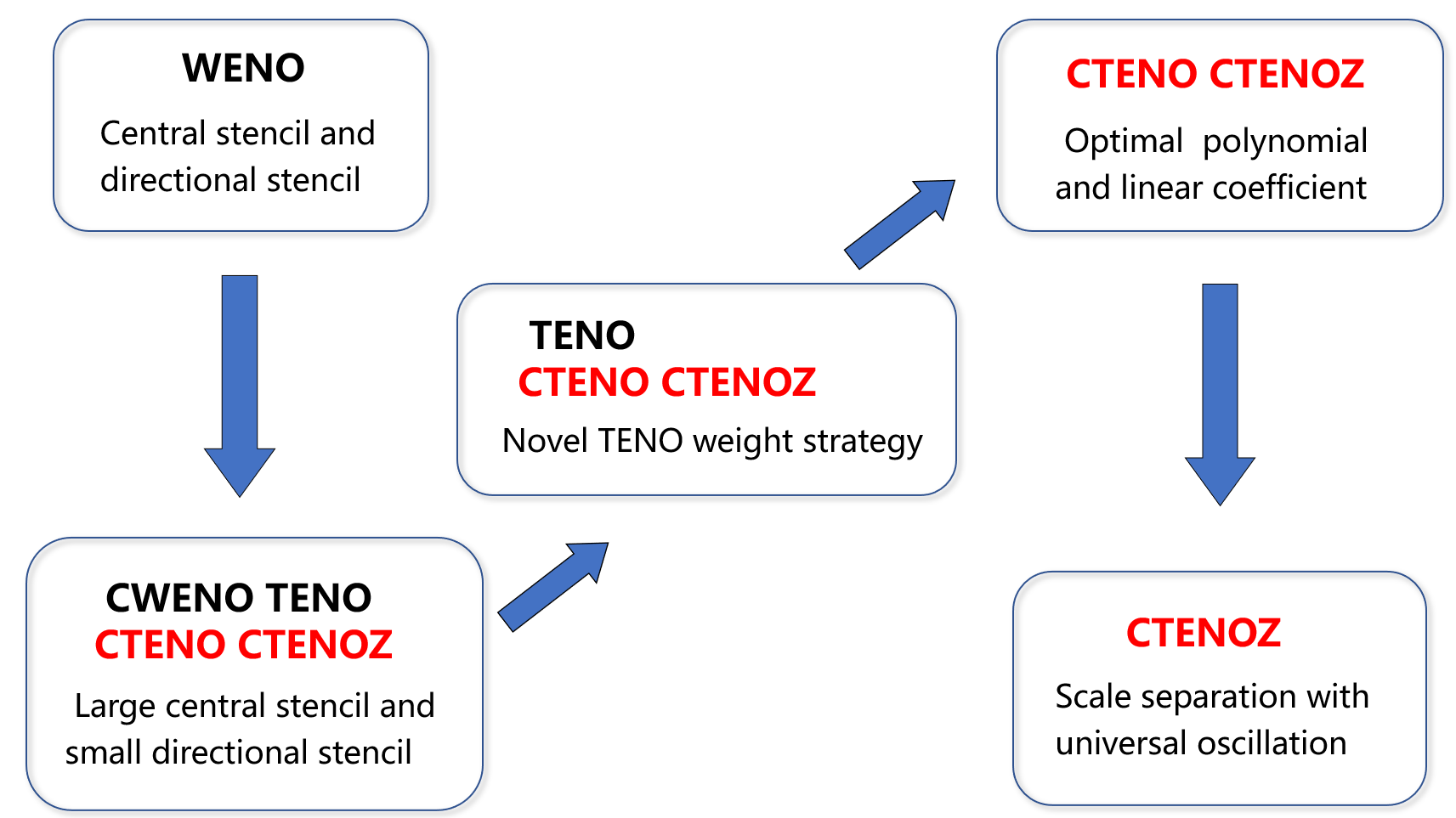
Fig. 2: The categorized features for WENO, CWENO, TENO, CTENO, and CTENOZ schemes are listed. The CTENO and CTENOZ shemes developed in this paper are marked in red.

2.7 Fluxes approximation

Harten-Lax-van Leer-Contact Riemann solver(HLLC)[50] is applied to inviscid fluxes, providing reliable approximations. The discontinuous left and right state $\mathbf{U}_{L}$ , $\mathbf{U}_{R}$ is

$$\mathbf{U}=\begin{cases}\mathbf{U}_{L},\text{ if }S_{L}>0\\ \mathbf{U}_{L}^{*},\text{ if }S_{L}\leq 0<S_{M}\\ \mathbf{U}_{R}^{*},\text{ if }S_{M}\leq 0<S_{R}\\ \mathbf{U}_{R},\ \text{ if }S_{R}<0\end{cases}$$ (31)

and the corresponding flux is

$$\mathbf{F}(\mathbf{U}_{L},\mathbf{U}_{R})=\begin{cases}\mathbf{F}_{L},\text{ if }S_{L}>0\\ \mathbf{F}_{L}^{*}=\mathbf{F}_{L}+S_{L}(\mathbf{U}_{L}^{*}-\mathbf{U}_{L}),\text{ if }S_{L}\leq 0<S_{M}\\ \mathbf{F}_{R}^{*}=\mathbf{F}_{R}+S_{R}(\mathbf{U}_{R}^{*}-\mathbf{U}_{R}),\text{ if }S_{M}\leq 0<S_{R}\\ \mathbf{F}_{R}.\ \text{ if }S_{R}<0\end{cases}$$ (32)

where $\mathbf{F}_{L}=\mathbf{F}(\mathbf{U}_{L})$ and $\mathbf{F}_{L}=\mathbf{F}(\mathbf{U}_{L})$. The acoustic wave-speed are evaluated by

$$S_{L}=min(u_{L}-c_{L},\tilde{u}-\tilde{c}),\quad S_{R}=max(u_{R}+c_{R},\tilde{u}+\tilde{c}),$$ (33)

where

$$\begin{cases}D_{\rho}=\sqrt{\frac{\rho_{R}}{\rho_{L}}},\\ \tilde{u}=\frac{u_{L}+u_{R}D_{\rho}}{1+D_{\rho}},\\ \tilde{H}=\frac{H_{L}+H_{R}D_{\rho}}{1+D_{\rho}},\\ \tilde{c}=\sqrt{(\gamma-1)[\tilde{H}-\frac{1}{2}\tilde{u}^{2}]}.\ \end{cases}$$ (34)

In order to determine the state $\mathbf{U}_{L}^{*}$ and $\mathbf{U}_{R}^{*}$, it is assumed that

$$S_{M}=u^{*}=u_{L}^{*}=u_{R}^{*},\quad p^{*}=p_{L}^{*}=p_{R}^{*}.$$ (35)

The speed of the contact wave is calculated as

$$S_{M}=\frac{\rho_{R}u_{R}(S_{R}-u_{R})-\rho_{L}u_{L}(S_{L}-u_{L})+p_{L}-p_{R}}{\rho_{R}(S_{R}-u_{R})-\rho_{L}(S_{L}-u_{L})},\quad p^{*}=\rho_{L}(u_{L}-S_{L})(u_{L}-S_{M})+p_{L},$$ (36)

where

$$\begin{cases}\rho_{L}^{*}=\rho_{L}\frac{S_{L}-u_{L}}{S_{L}-S_{M}},\rho_{R}^{*}=\rho_{R}\frac{S_{R}-u_{R}}{S_{R}-S_{M}},\\ \rho_{L}^{*}u_{L}^{*}=\frac{(S_{L}-u_{L})\rho_{L}u_{L}+p^{*}-p_{L}}{S_{L}-S_{M}},\rho_{R}^{*}u_{R}^{*}=\frac{(S_{R}-u_{R})\rho_{R}u_{R}+p^{*}-p_{R}}{S_{R}-S_{M}},\\ \rho_{L}^{*}v_{L}^{*}=\frac{(S_{L}-u_{L})\rho_{L}v_{L}}{S_{L}-S_{M}},\rho_{R}^{*}v_{R}^{*}=\frac{(S_{R}-u_{R})\rho_{R}v_{R}}{S_{R}-S_{M}},\\ \rho_{L}^{*}w_{L}^{*}=\frac{(S_{L}-u_{L})\rho_{L}w_{L}}{S_{L}-S_{M}},\rho_{R}^{*}w_{R}^{*}=\frac{(S_{R}-u_{R})\rho_{R}w_{R}}{S_{R}-S_{M}},\\ E_{L}^{*}=\frac{(S_{L}-u_{L})E_{L}-p_{L}u_{L}+p^{*}S_{M}}{S_{L}-S_{M}},E_{R}^{*}=\frac{(S_{R}-u_{R})E_{R}-p_{R}u_{R}+p^{*}S_{M}}{S_{R}-S_{M}}.\ \end{cases}$$ (37)

In the subsequent section, the HLLC method is utilized as the Riemann solver, which has been proven to possess robustness and reliability for the Euler equations.

3 Numerical tests

The effectiveness of proposed CTENO and CTENOZ schemes will be assessed through a set of numerical simulations. We perform various benchmark test problems that involve both smooth and discontinuous solutions. The evaluation focuses on the performance of the CTENO and CTENOZ scheme in capturing interfaces in the inviscid compressible Euler equations. Several test problems are listed below:

• Accuracy Order Tests: This test problem evaluates the accuracy and errors of the methods in verifying the designed order of accuracy.

• Shock-tube problem: This test examines the effectiveness of proposed schemes by comparing their solutions to the exact Sod problem, demonstrating their capability to accurately capture discontinuities.

• Shock-density wave interaction: This test problem evaluates the non-oscillatory characteristics when combined with smooth flow features. The impact of the linear weight of the central stencil is also take into account.

• 2D Double Mach Reflection of a Strong Shock: This test problem evaluates the ability to capture discontinuities and the properties of dissipation. The refined mesh is considered and the computational cost is compared among different schemes. The parallel scalability is tested on the refined mesh.

• Single-Material Triple Point Problem: This test problem assesses the efficiency in capturing interfacial instability and smaller-scale structure. The computational cost associated with different orders is also investigated.

• Kelvin-Helmholtz instability: This problem serves as a test to evaluate the precision and dissipation characteristics of numerical techniques. The dissipation of total kinetic energy is examined to assess the performance of schemes.

• Interaction of a Shock Wave with a Wedge in 2D: This test problem is used to assess the performance involving strong gradients that interact with vortices, and compare it with the experimental results.

• Helium Bubble Shock Wave: This test problem is utilized to evaluate the capability of simulating multicomponent flow. The results is compared to experiment, revealing the interaction between shock waves and bubbles.

3.1 Accuracy Order Tests

We consider the two-dimensional Euler equations, the initial conditions of the test are $\rho(x,y,0)=1+0.2sin(2\pi(x+y))$, $u(x,y,0)=1$, $v(x,y,0)=1$, $p(x,y,0)=1$. The computational domain is $[0,1]\times[0,1]$, and periodic boundary conditions are employed. The exact solution of the density is $\rho(x,y,t)=1+0.2sin(2\pi(x+y-2t))$. The numerical errors $L^{2}error$ and $L^{\infty}error$ are calculated by:

$$L^{2}error=\sqrt{\frac{\sum_{i}\int_{V_{i}}(U_{e}(x,t)-U_{c}(x,t))^{2}dV}{\sum_{i}\mid V_{i}\mid}},$$ (38)

$$L^{\infty}error=Max\mid U_{e}(x,t)-U_{c}(x,t)\mid,$$ (39)

where $U_{e}(x,t)$ and $U_{c}(x,t)$ are the exact and numerical results at the end of simulation. We select a large central stencil linear weight of $\lambda_{1}^{{}^{\prime}}=10^{15}$ to fully utilize the capabilities of high order polynomials.[30]. The errors and numerical accuracy orders at time $t=1$ are displayed in Table 1. After simulating the smooth indicators of each stencil, the CTENO and CTENOZ schemes provide the same error and accuracy order due to the choice of large center stencil in smooth areas. In the case of two dimensions Euler equations, it is observed that the theoretical order of accuracy and errors are achieved. The CTENO and CTENOZ schemes demonstrate the designed convergence order for both $L^{2}error$ and $L^{\infty}error$.

Table 1: Errors and accuracy with two dimensional Euler equations for CTENO and CTENOZ schemes. $h$ is the number of edges. $Ne$ is the total number of elements. Both $L^{\infty}error$ and $L^{2}error$ are calculated based on $h$ and $Ne$.

	$h$	$Ne$	$L^{\infty}error$	$L^{\infty}order$	$L^{2}error$	$L^{2}order$
CTENO3	1/10	100	1.06E-01		7.54E-02
CTENOZ3	1/16	256	3.60E-02	2.29	2.57E-02	2.29
	1/20	400	1.97E-02	2.70	1.40E-02	2.71
	1/32	1024	5.11E-03	2.87	3.63E-03	2.88
	1/40	1600	2.65E-03	2.95	1.88E-03	2.95
CTENO4	1/10	100	5.39E-02		3.72E-02
CTENOZ4	1/16	256	1.02E-02	3.55	6.95E-03	3.57
	1/20	400	4.32E-03	3.84	2.96E-03	3.83
	1/32	1024	6.80E-04	3.93	4.71E-04	3.91
	1/40	1600	2.80E-04	3.97	1.95E-04	3.95
CTENO5	1/10	100	2.31E-02		1.63E-02
CTENOZ5	1/16	256	2.56E-03	4.68	1.83E-03	4.65
	1/20	400	8.69E-04	4.84	6.19E-04	4.87
	1/32	1024	8.58E-05	4.92	6.08E-05	4.94
	1/40	1600	2.84E-05	4.96	2.00E-05	4.97
CTENO6	1/10	100	1.33E-02		9.10E-03
CTENOZ6	1/16	256	9.22E-04	5.67	6.35E-04	5.67
	1/20	400	2.48E-04	5.88	1.71E-04	5.89
	1/32	1024	1.48E-05	6.00	1.03E-05	5.97
	1/40	1600	3.88E-06	6.00	2.69E-06	6.01
CTENO7	1/10	100	9.52E-03		6.63E-03
CTENOZ7	1/16	256	3.15E-04	7.25	2.24E-04	7.21
	1/20	400	6.87E-05	6.82	4.88E-05	6.83
	1/32	1024	2.71E-06	6.88	1.89E-06	6.91
	1/40	1600	6.08E-07	6.70	4.07E-07	6.89

3.2 Shock-tube problem

The 1D shock-tube problem has been extensively employed for evaluating implementation of numerical methods[51]. The provided initial conditions are detailed below:

$$(\rho,u,p)=\begin{cases}(1,0,0.1),\ -0.5\leq x<0\\ (0.125,0,0.1).\ 0\leq x\leq 0.5\end{cases}$$ (40)

The computational domain spans from $[-0.5,0.5]\times[0,0.2]$. In this case, unstructured elements are utilized with an approximate resolution of $h\approx 1/68$. The high-order reconstruction uses characteristic variables. The simulation is conducted on an unstructured mesh comprising of 2112 uniformly triangular cells. The ultimate computation time is set at $t=0.2$.

The profiles of density and velocity acquired from the CTENO and CTENOZ of varies orders are presented in Fig. 3, effectively capturing the discontinuities without any spurious oscillations. The precise solution to the Sod shock tube was obtained from Riemann problem. Fig. 4 presents solutions of density and velocity distributions using different schemes. These results from all schemes exhibit good agreement with the exact solution, accurately capturing discontinuity and shock wave. However, the CTENO and CTENOZ scheme demonstrate higher accuracy compared to the CWENO and TENO scheme near the discontinuities.

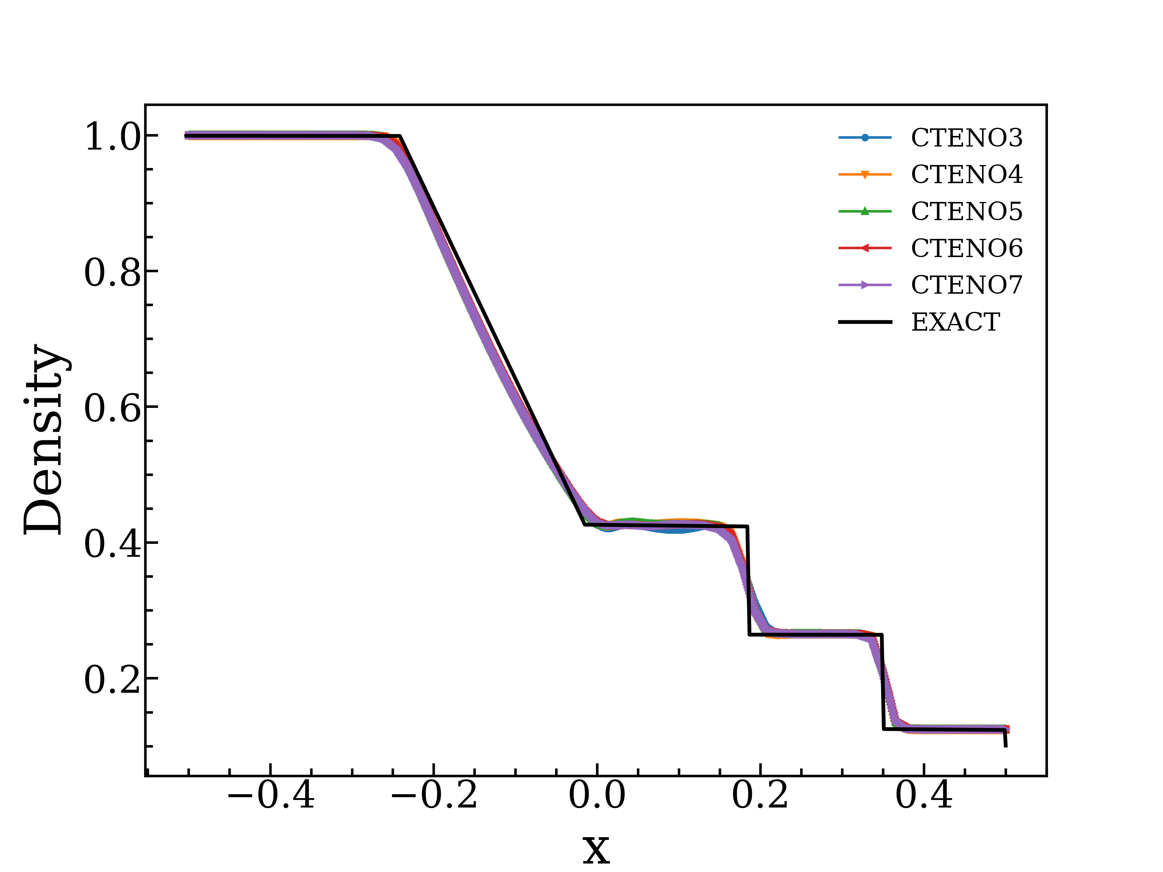
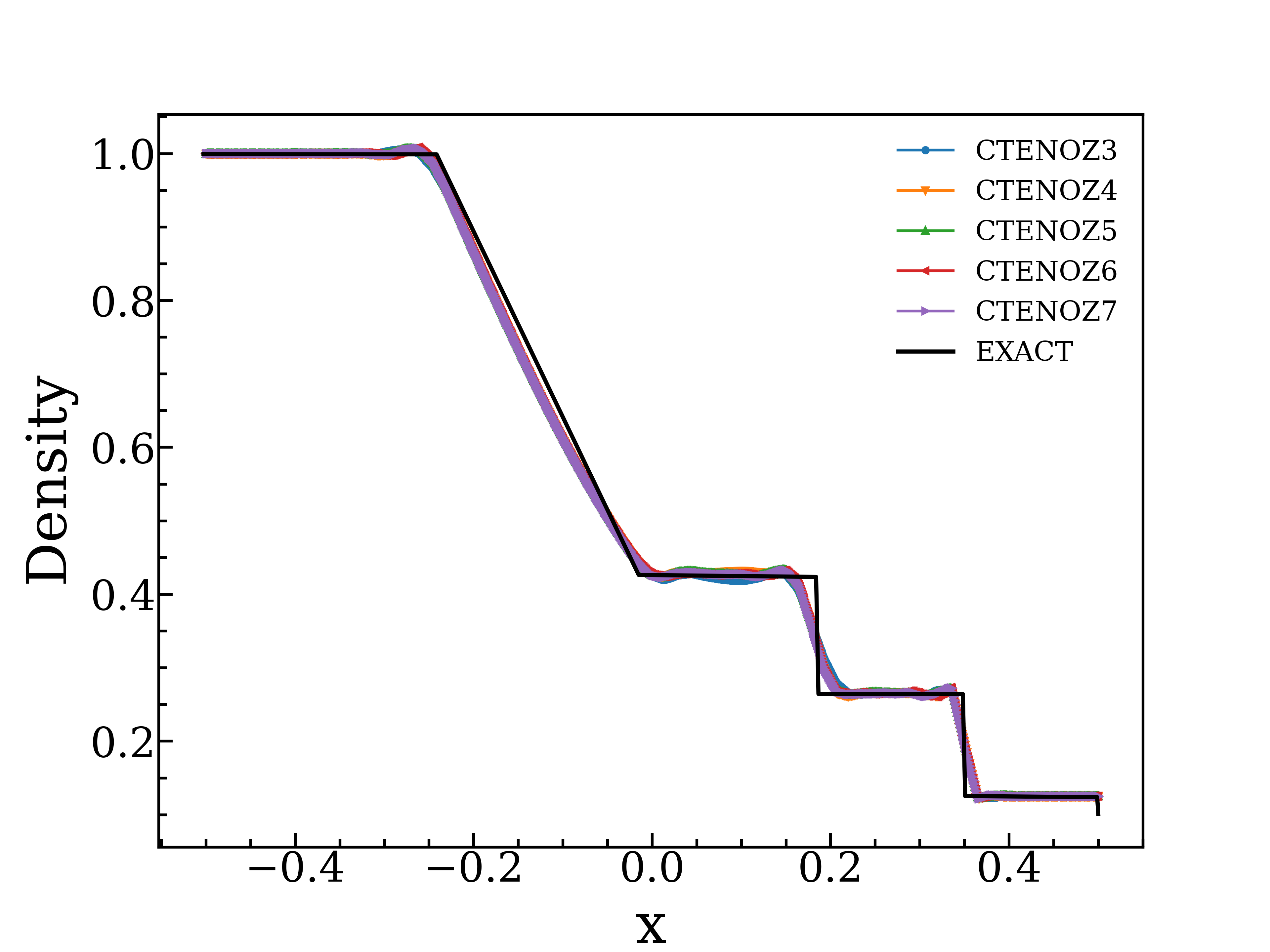
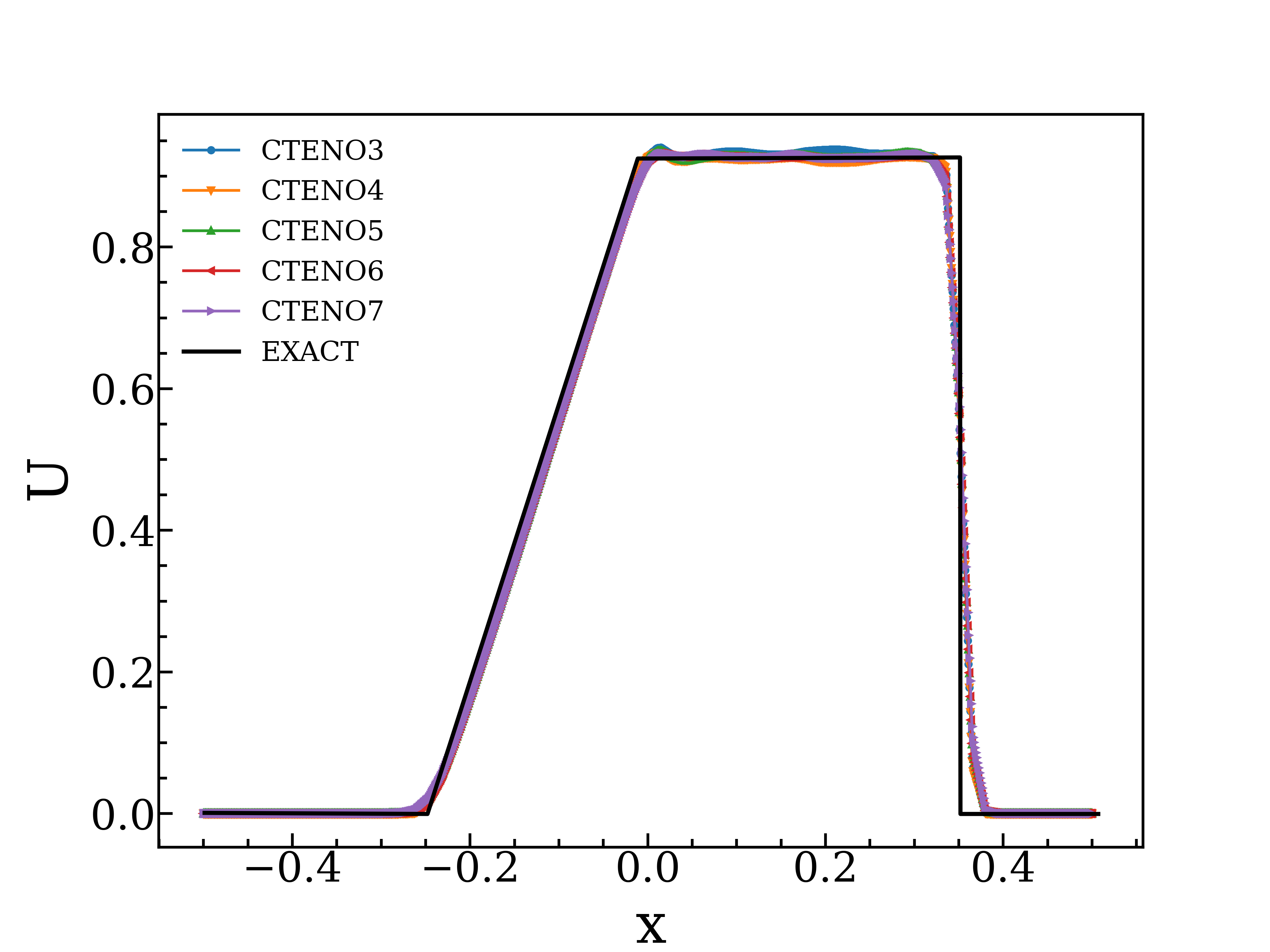
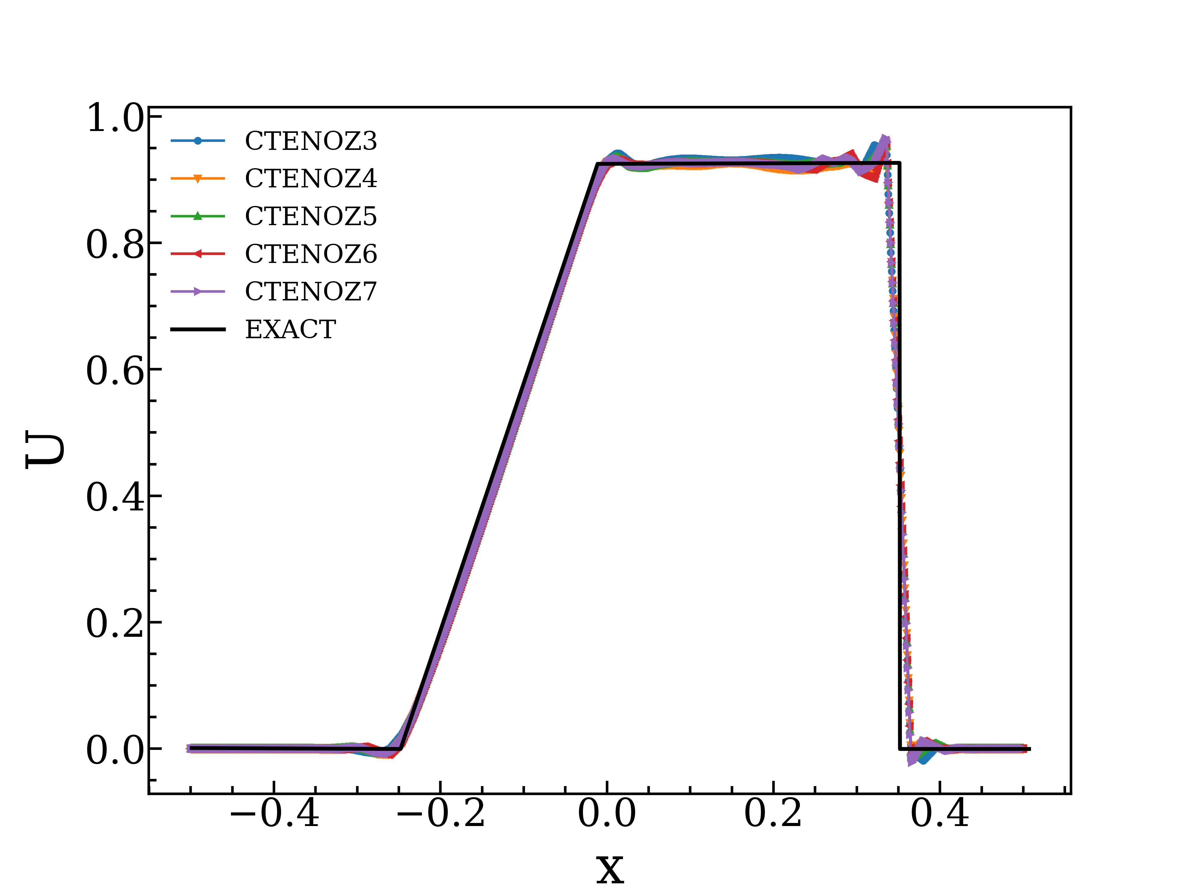
Fig. 3: shock-tube problem: solutions from CTENO and CTENOZ schemes of different orders. Density and velocity profiles are compared with precise solution.

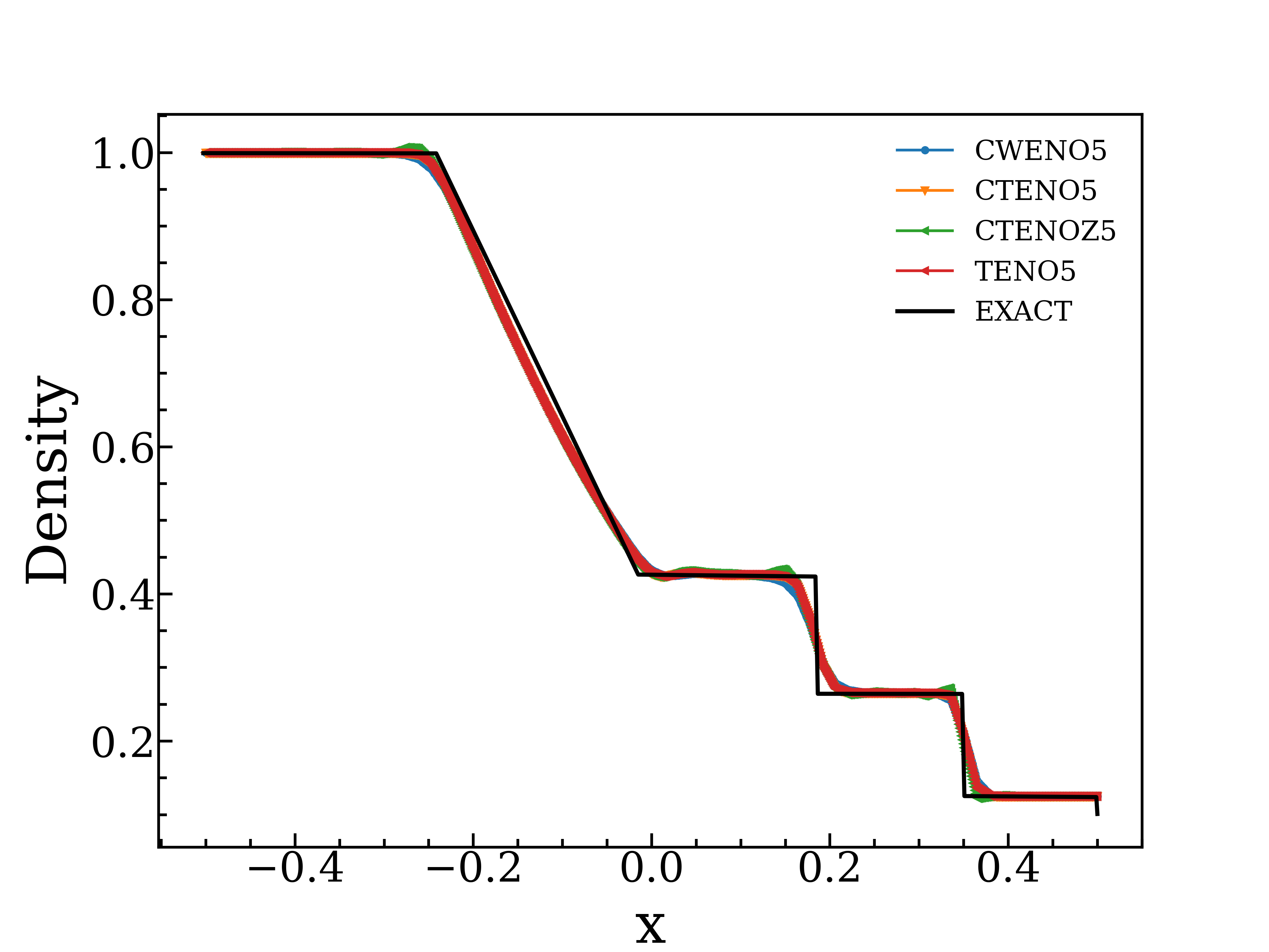
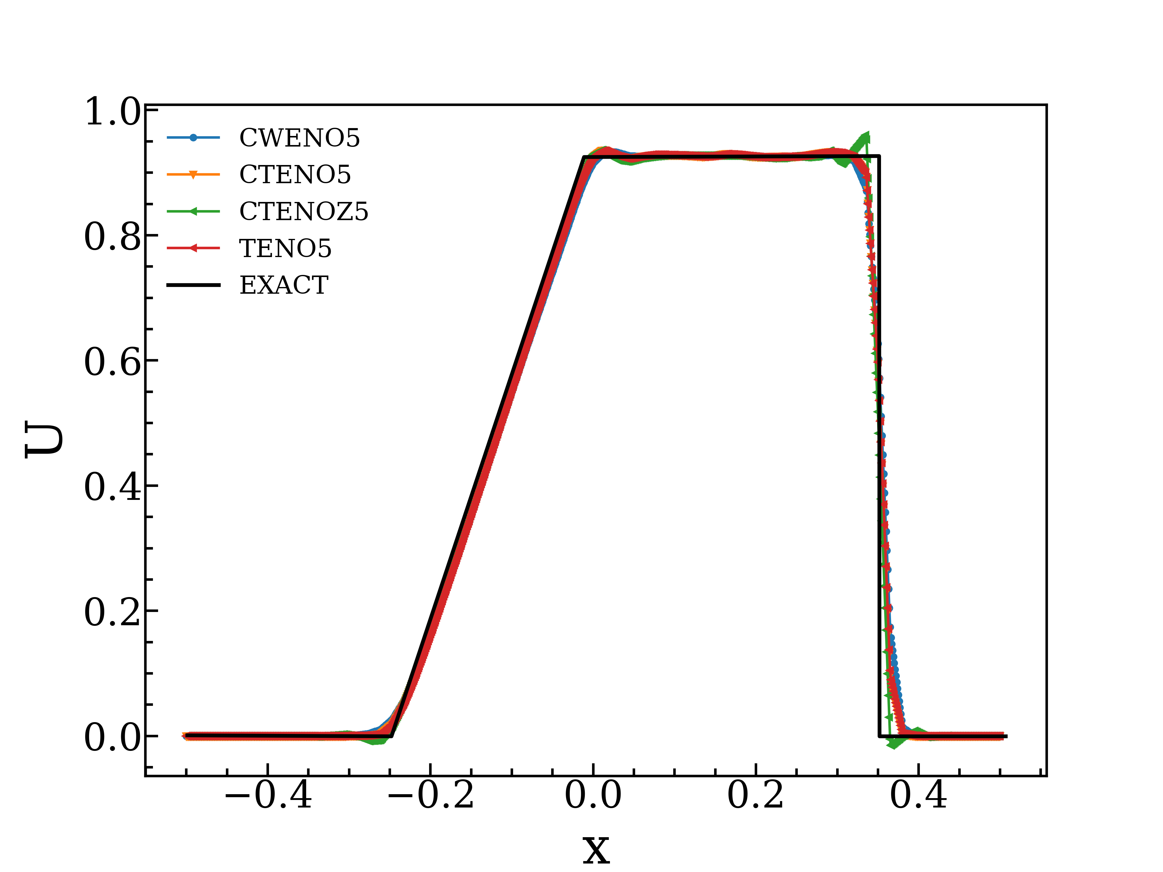
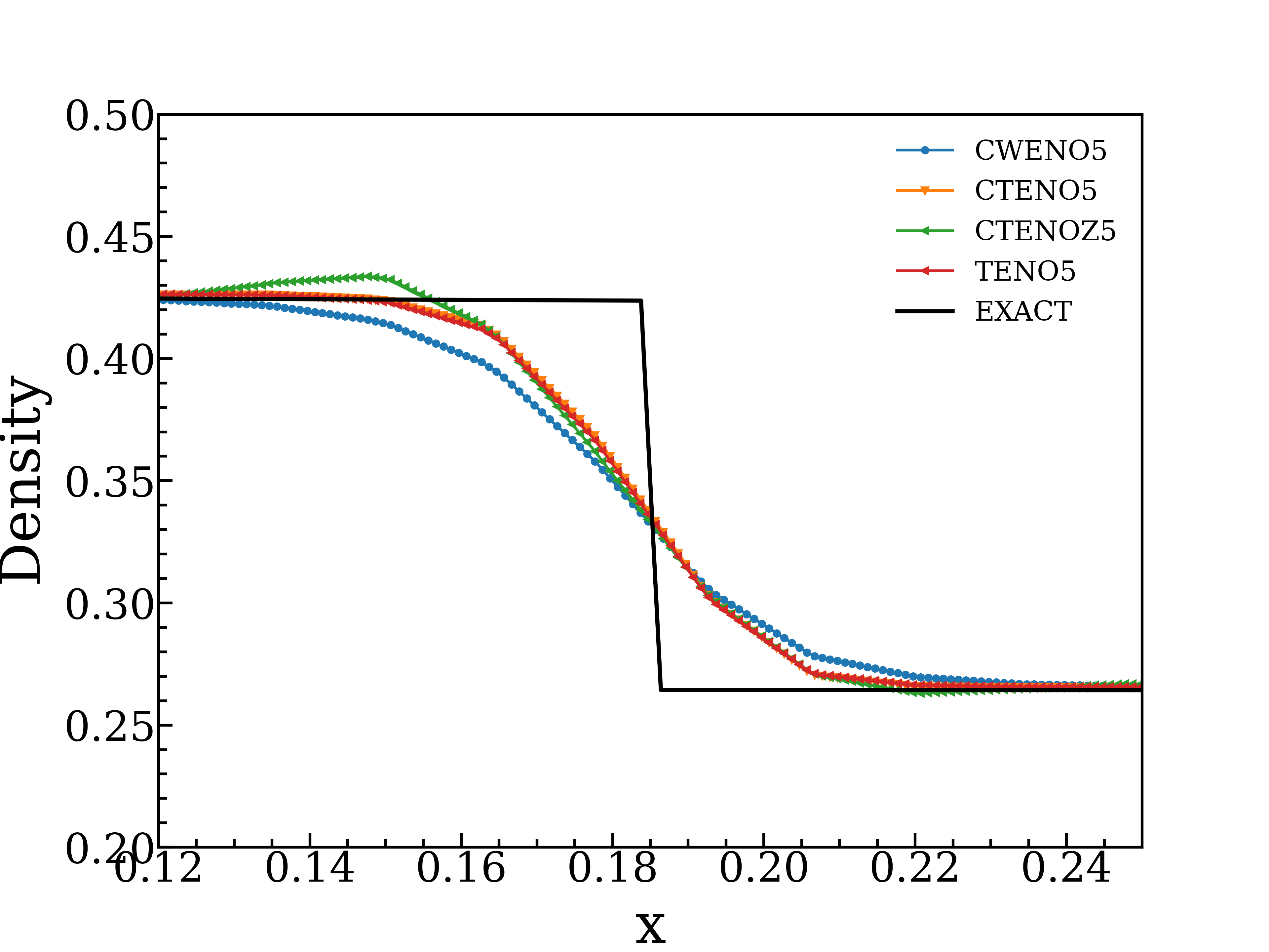
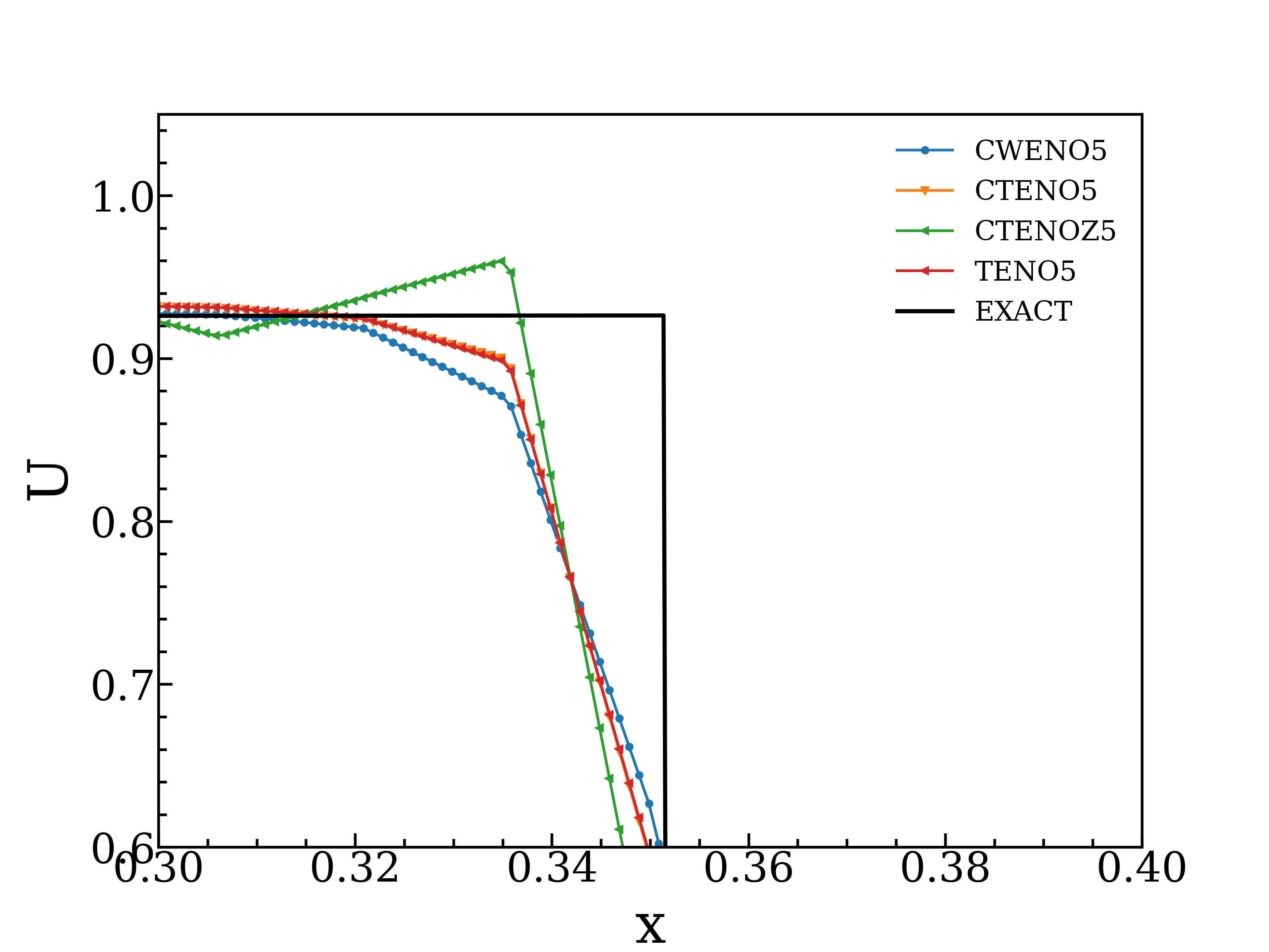
Fig. 4: shock-tube problem: solutions from CWENO,TENO,CTENO and CTENOZ schemes with 5th-order. Density and velocity profiles are compared with precise solution.

3.3 Shock-density wave interaction

The problem of shock-density wave interaction focus on a 1D shock wave with Mach number $3$ and disturbed density field, as proposed in [52]. This interaction results in the development of structures and discontinuities in small-scale. Consequently, this test problem is commonly utilized to assess abilities to capture shock waves and resolve wave numbers with different numerical methods. The initialization of flow field is

$$(\rho,u,p)=\begin{cases}(3.8571,2.6294,10.333),\ -5\leq x<-4\\ (1+0.2sin(5x),0,1).\ -4\leq x\leq 5\end{cases}$$ (41)

The computational domain is $[-5,5]\times[0,2]$ and consists of 18282 triangular mesh cells distributed in a uniform manner, approximately with $h\approx 1/20$. The time of the ultimate evolution is $t=1.8$. To obtain an accurate reference solution, a 1D Euler equations is utilized, with $2000$ grid nodes and WENO scheme of 5th order. Fig. 5(a) illustrates the successful capture of sound waves and small shocklets with robustness in various schemes. Regarding the entropy wave in the same accuracy order, the CTENO and CTENOZ schemes display a notable enhancement in comparison with CWENO and TENO. This improvement is attributed to their superior preservation of the density wave amplitude. The CWENO demonstrate highest dissipation, resulting in dissipation of certain structures with small-scale. Among all schemes presented by Fig. 5(a), CTENOZ schemes shows the least dissipation and better performance than other schemes. The CTENOZ schemes show higher order of accuracy with the increase of different orders an shown in Fig. 5(b).

According to Tsoutsanis and Dumbser[30], CWENO schemes have the flexibility to choose different values of central stencil linear weight $\lambda_{1}^{{}^{\prime}}$. When dealing with problems involving strong discontinuities, using a too large $\lambda_{1}^{{}^{\prime}}$ often leads to simulation failure and sacrifices robustness. To conduct a comprehensive comparison of CTENO and CTENOZ schemes with different values of $\lambda_{1}^{{}^{\prime}}$, the density profiles of CTENO and CTENOZ schemes with values of $10^{3}$, $10^{4}$, $10^{5}$, and $10^{6}$ are presented in Fig. 6. In CTENO schemes, it can be observed that larger $\lambda_{1}^{{}^{\prime}}$ values provide better resolution for high-wavenumber fluctuations, similar to the conclusion tested in CWENO schemes through numerical experiments. The CTENOZ schemes achieve almost identical results, while not being sensitive to the choice of $\lambda_{1}^{{}^{\prime}}$. The insensitivity to the central stencil linear weight can be attributed to the scaling of smoothness indicators provided by polynomials of various orders. To achieve a harmonious equilibrium between performance and robustness, a uniform $\lambda_{1}^{{}^{\prime}}$ value of $10^{4}$ is adopted for CTENO schemes in this paper.

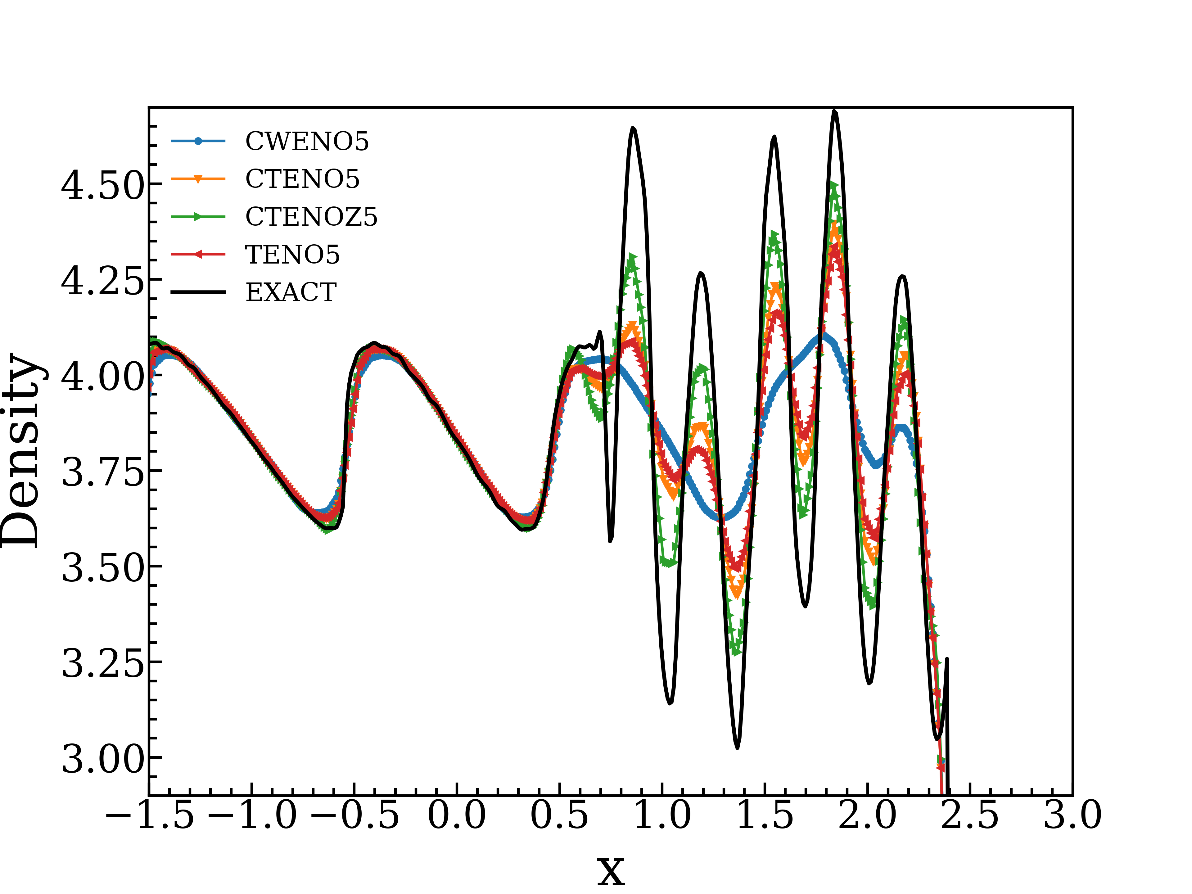
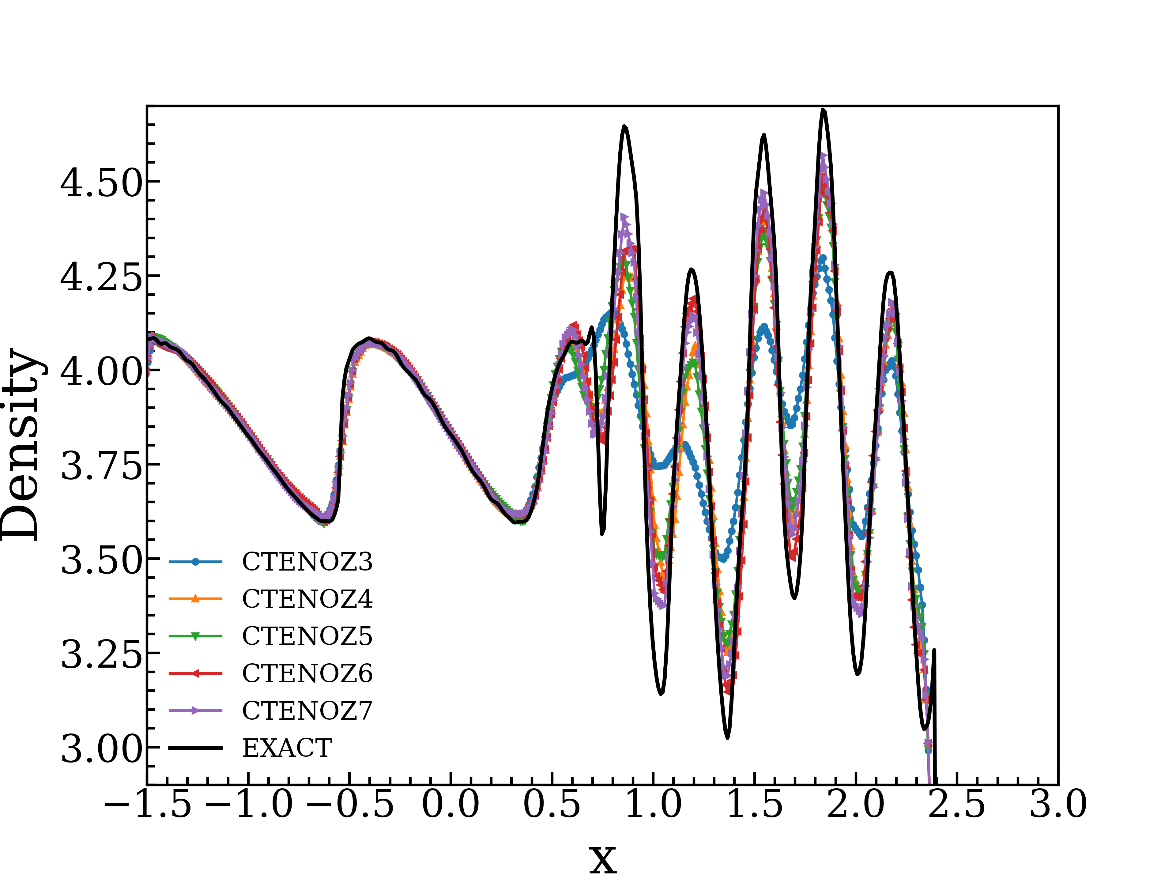
Fig. 5: shock-density wave interaction: solutions from (a) CWENO, TENO ,CTENO and CTENOZ of 5th-order,(b) CTENOZ scheme of various orders. Density profiles are compared with reference solution.

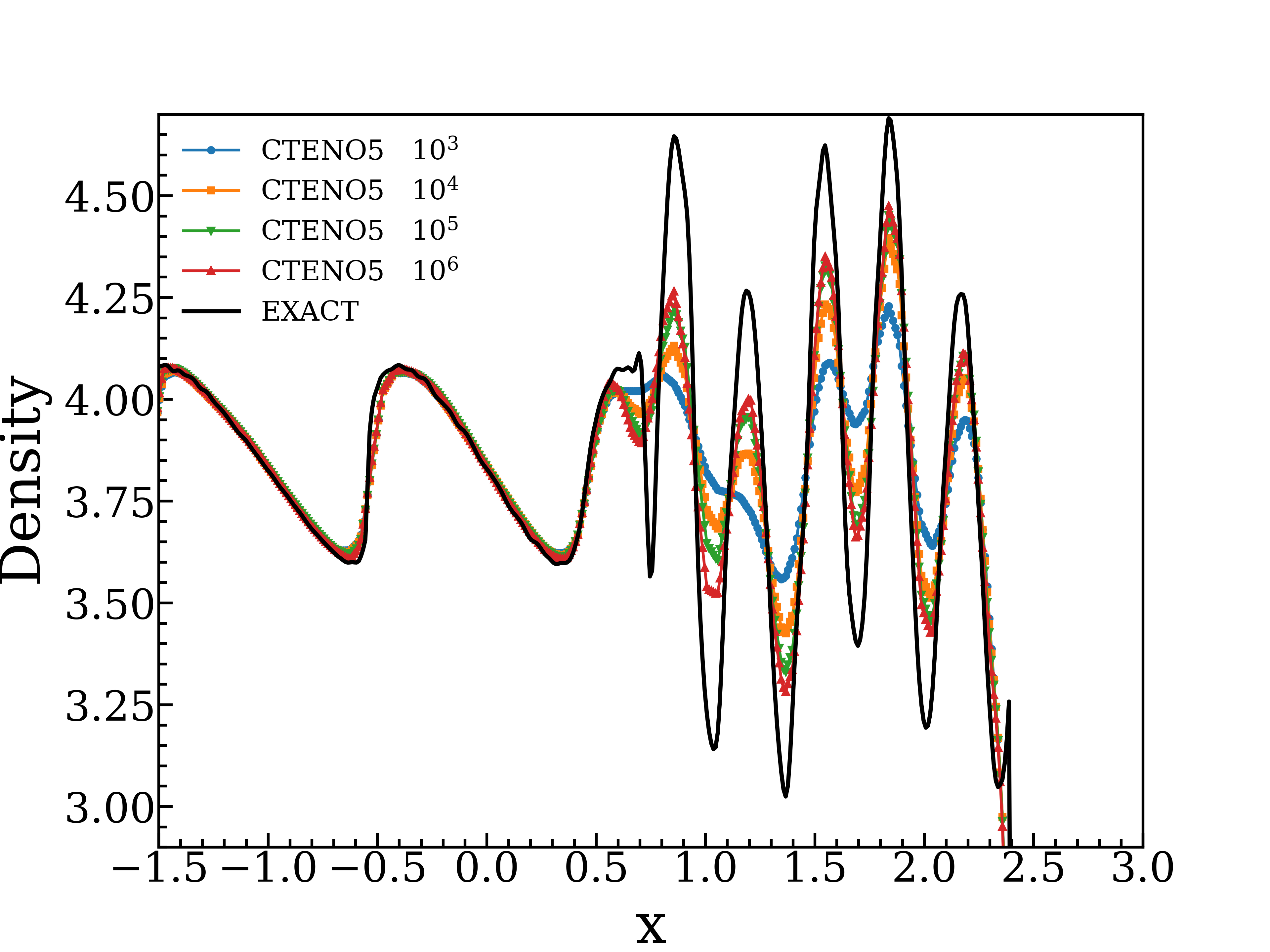
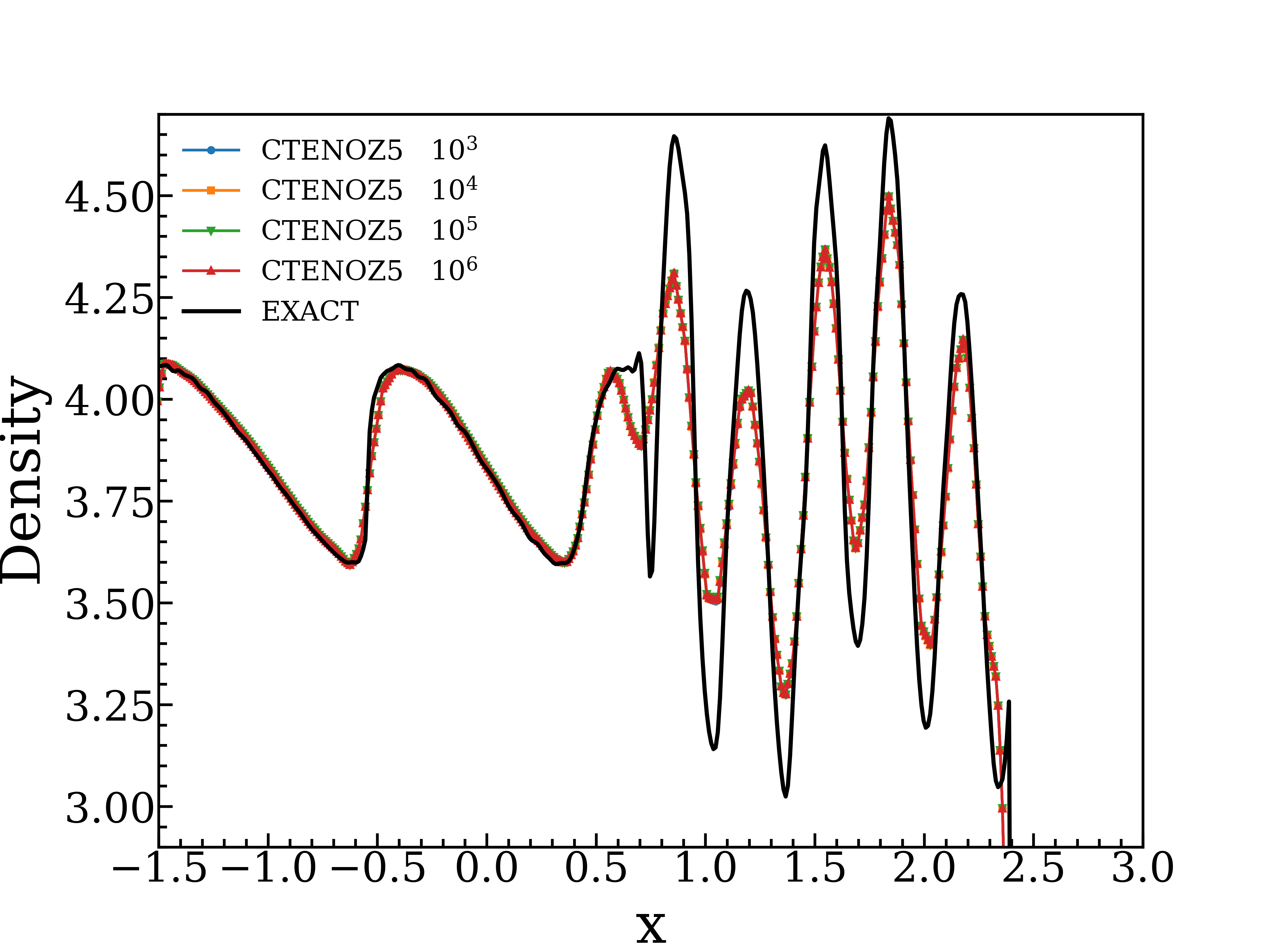
Fig. 6: shock-density wave interaction: 5th-order solutions from CTENO and CTENOZ with different $\lambda_{1}^{{}^{\prime}}$. Density profiles are compared with reference solution.

3.4 2D Double Mach Reflection of a Strong Shock

This classical 2D double Mach reflection of a strong shock is referenced from [53]. It is commonly employed for assessing the properties of dissipation and capability to capture discontinuous. The initialization of computational domain is:

$$\begin{array}[]{c}(\rho,u,v,p)=\begin{cases}(1.4,0,0,1),\ \text{ if }y<1.732(x-0.1667)\\ (8,7.145,-4.125,116.8333).\ \text{ otherwise }\end{cases}\end{array}$$ (42)

The computational domain spans from $[0,4]\times[0,1]$ and consists of 369604 and 714138 uniformly distributed triangular cells, with each cell approximately $h\approx 1/200$ and $h\approx 1/278$. The simulation runs until $t=0.2$. A shock wave with Mach number of $10$ originates from $x=0.1667$ and has an incident angle of $60$ degrees relative to $x$-axis, travels towards right. The initial state of post-shock is enforced from $x=0$ to $x=0.1667$, while wall boundary condition is applied from $x=0.1667$ to $x=4$ at bottom. The fluid are defined at the top to accurately capture the behavior of shockwave.

Fig. 7 and Fig. 8 illustrates the numerical results for 5th and 7th orders of CTENO and CTENOZ schemes and their respective CWENO and TENO schemes. As shown in Fig. 7 and Fig. 8 , for the same mesh resolution, higher-order CTENO and CTENOZ schemes can accurately capture small-scale features with greater precision and reduced numerical dissipation, while the CTENOZ schemes shows the best performance. The density distributions reveals the absence of any erroneous numerical oscillations near the discontinuities. It is important to highlight that CWENO, TENO, CTENO, and CTENOZ schemes demonstrate robustness across all tested mesh resolutions, with their robustness outperforming the WENO scheme [54]. The region surrounding the double Mach stems showed significant variations in the results, with CTENO and CTENOZ demonstrating lower dissipation and facilitating improved identification of small-scale vortex structures. Overall, the CTENO and CTENOZ scheme outperformed the CWENO and TENO schemes in terms of performance. Similarly, the current simulation results exhibit a high degree of similarity to the results obtained using a more refined mesh.

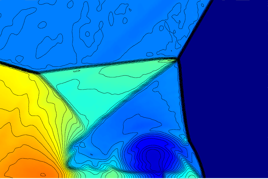
(a) CWENO5

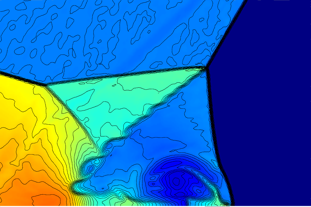
(b) TENO5

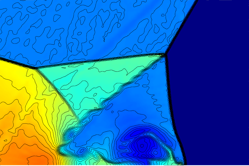
(c) CTENO5

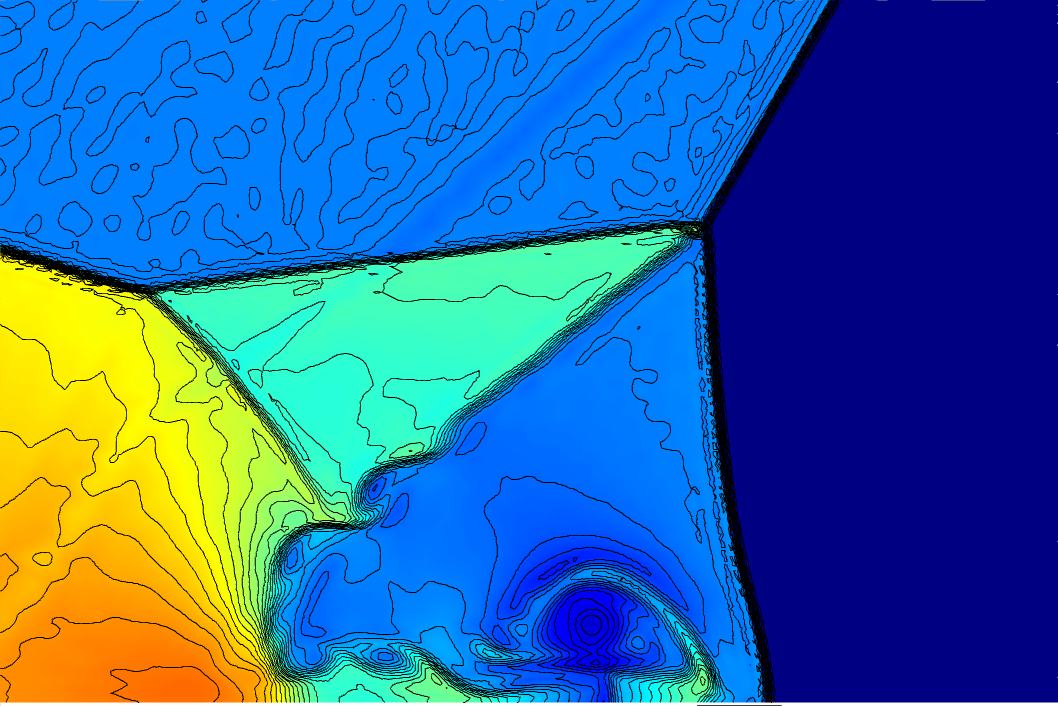
(d) CTENOZ5

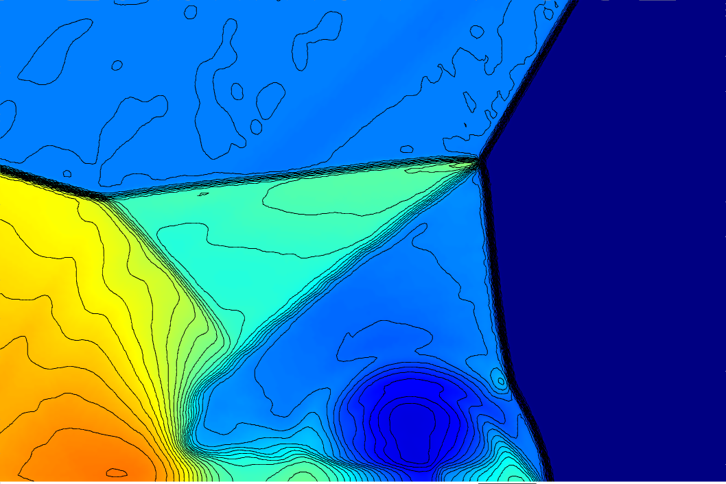
(e) CWENO7

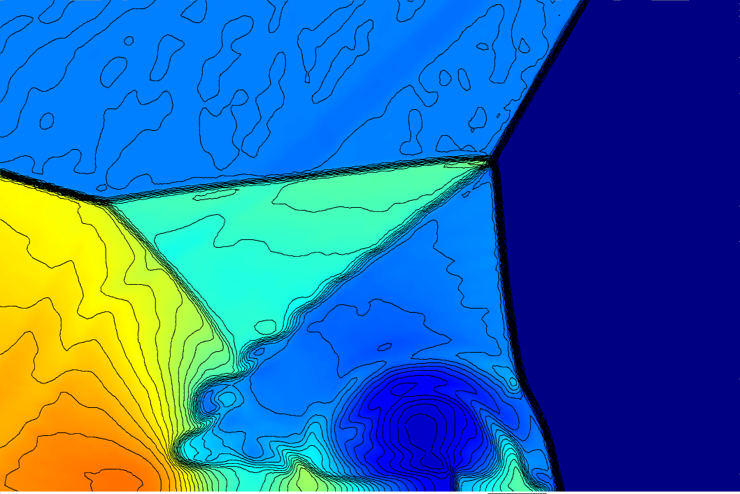
(f) TENO7

(g) CTENO7

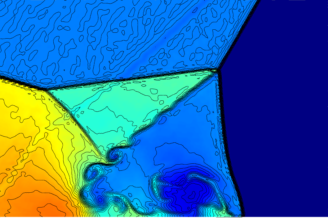
(h) CTENOZ7

Fig. 7: 2D double Mach reflection of a strong shock: results from (a) CWENO5, (b) TENO5,(c)CTENO5,(d) CTENOZ5,(e) CWENO7 ,(f)TENO7,(g)CTENO7 and (h)CTENOZ7. The figures contain 50 density contours ranging from 2 to 23. The mesh consists of 369604 uniform triangular cells.

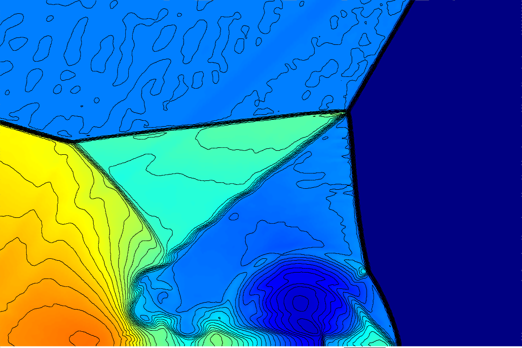
(a) CWENO5

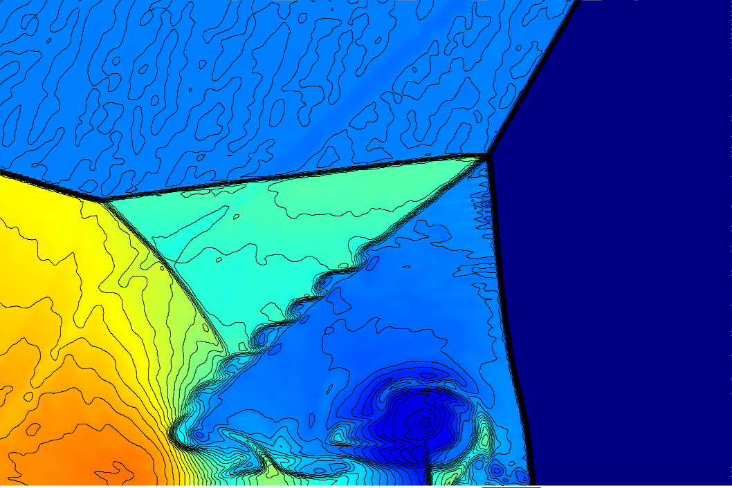
(b) TENO5

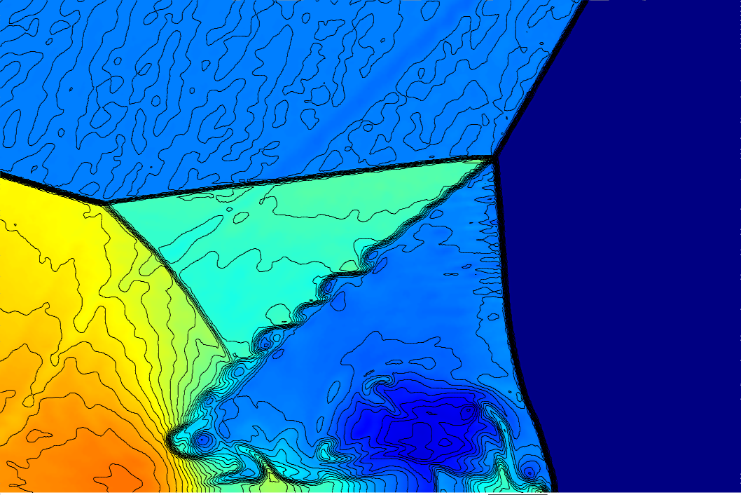
(c) CTENO5

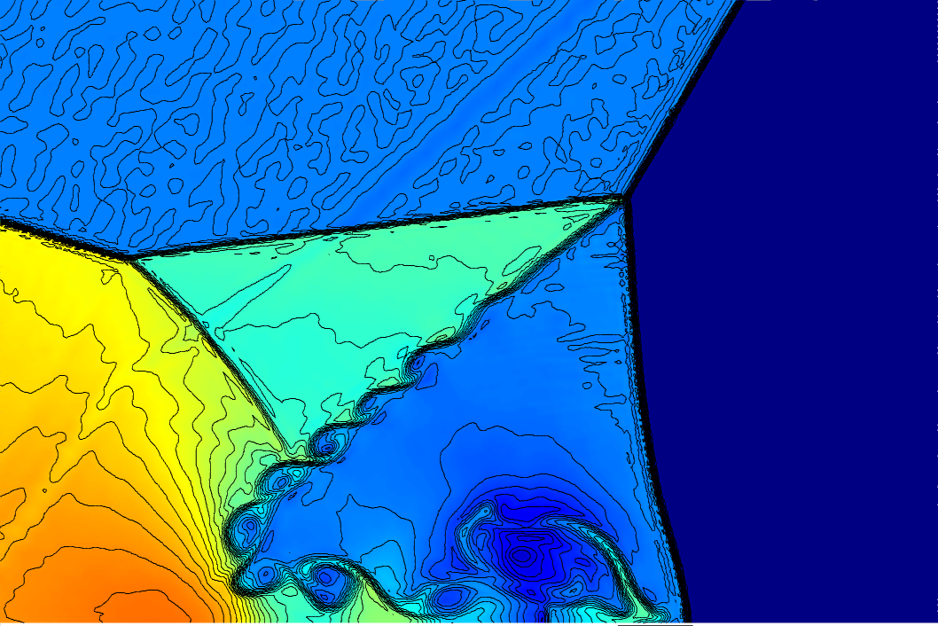
(d) CTENOZ5

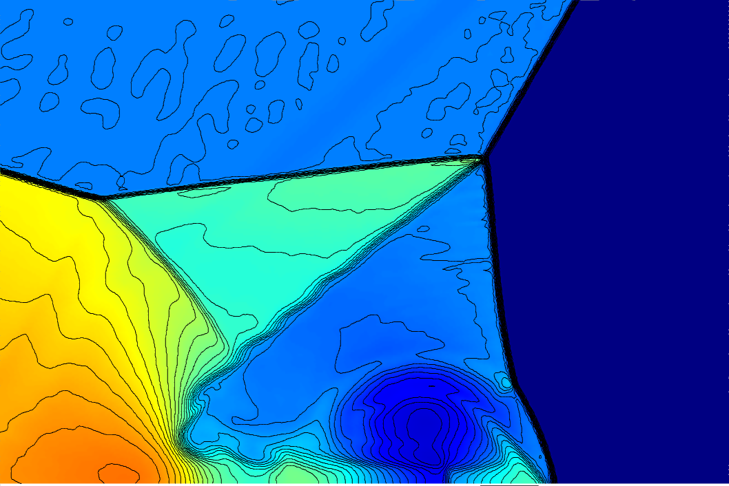
(e) CWENO7

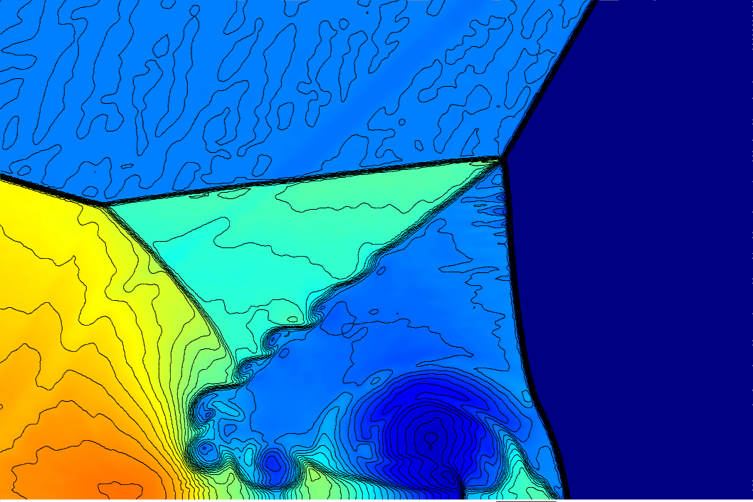
(f) TENO7

(g) CTENO7

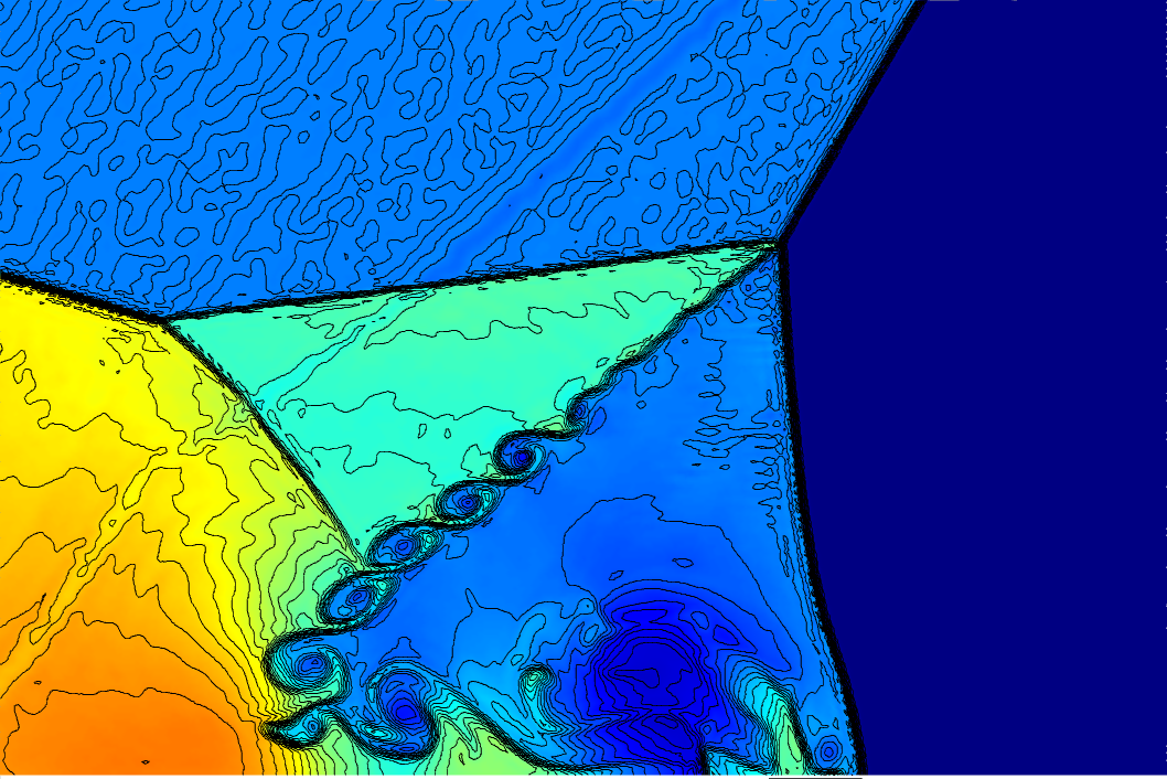
(h) CTENOZ7

Fig. 8: 2D double Mach reflection of a strong shock: results from (a) CWENO5, (b) TENO5,(c)CTENO5,(d) CTENOZ5,(e) CWENO7 ,(f)TENO7,(g)CTENO7 and (h)CTENOZ7. The figures contain 50 density contours ranging from 2 to 23. The mesh consists of 714138 uniform triangular cells.

3.4.1 run time

The computational times presented in 2D double Mach reflection were derived from identical hardware (and compilation settings) and standardized against a reference setup on the same hardware. This normalization allows for a fair comparison of algorithm performance under identical hardware conditions. The benefits of the CWENO schemes, in contrast to the WENO scheme, are not solely limited to reduced computational time but also exhibit significantly improved robustness [30, 31]. In this particular test, the CWENO ,TENO, CTENO, and CTENOZ scheme require approximately the same amount of time with the same spatial order, as shown in Table 2.

Table 2: Normalised computational times (with respect to CWENO 5th order with 369604 uniform triangular elements) for 2D Double Mach Reflection test problem.

Elements	CWENO5	TENO5	CTENO5	CTENOZ5
369604	1.000	1.036	1.033	1.000
714138	2.798	2.870	2.795	2.811

3.4.2 Parallel scalability

The performance of parallelization for existing methods and computer code was evaluated by implementing the 2D double Mach reflection flow case with the finest mesh consisting of 714138 triangular elements. Grid partitioning was performed using the METIS software[36]. The numerical methods used in this study were incorporated into Fortran 90 code, which employed the Message Passing Interface (MPI) for parallel communications. The performance tests were conducted at the Beijing Super Cloud Computing Center (BSCC) facility. The numerical experiments were carried out on the AMD EPYC 7542 CPU model. The maximum computational time for 2000 iterations was recorded for all test cases.

The original code implementation shows that the calculation of WENO weights takes up the most time, followed by least-square reconstruction and extrapolation of flow variables and gradients at cell interfaces. When considering communication expenses, the most expensive aspect lies in communication of the reconstructed solutions and their gradients for the Gaussian quadrature points between inter-processor boundaries, rather than communication of the solutions for the stencil elements across inter-processor boundaries. Therefore, the calculation of WENO weights has been recognized as having the capability to greatly improve the performance of the CFD code[37]. This research focuses on examining the weights calculation of CTENO and CTENOZ schemes in order to assess their parallel performance.

The reference time for normalizing the CPU results of the numerical simulations was calculated based on the time required for one time-iteration of the CTENO-5th order scheme on 64 processors. To assess the scalability of the methods and computer code, experiments were conducted with the number of processors ranging from 64 to 1024. As the numerical accuracy order increases, the computational time increases at a faster rate compared to the communication time, indicating that higher-order numerical schemes exhibit better scalability than lower-order schemes. This is illustrated inFig. 9.

The parallelization of the unstructured schemes involves interprocessor communication for exchanging two types of data: (i) the cell-centered values of halo elements on the stencil, and (ii) the reconstructed, boundary extrapolated values of Gaussian quadrature points on the direct-side halo neighboring elements. The second communication requirement is commonly found in high-order schemes. The amount of data needed for (i) is much smaller compared to (ii) because the latter involves the boundary extrapolated values of the solution and solution gradients (for viscous flows) at each surface Gaussian quadrature point. For the CTENO-5th order scheme, the wall-clock time per iteration is 1.7s on 64 processors, and for the CTENO-7th order scheme, it is approximately 1.5 times higher. When the number of processors increases from 64 to 128, 256, 512, 1024, the iteration time decreases, resulting in an approximately 2.0 times speedup in practice Fig. 9.

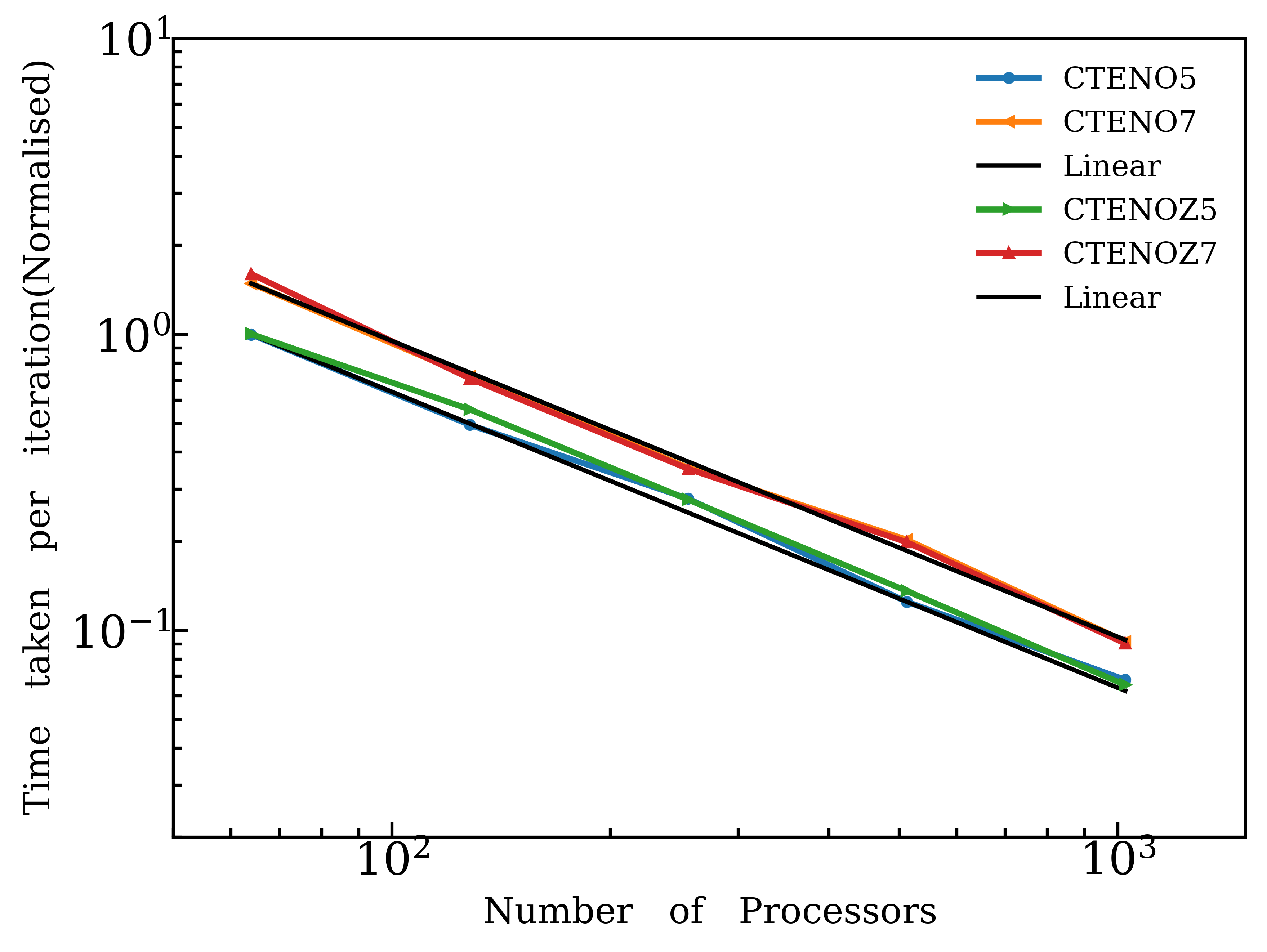
Fig. 9: Parallel scalability of CTENO5, CTENO7, CTENOZ5 and CTENOZ7 numerical schemes for the 2D double Mach reflection.

3.5 Single-Material Triple Point Problem

We examine single-material triple point problem and adopt the configuration outlined in [55]. The simulation region is $[0,7]\times[0,3]$ and initialization is specified as follows

$$\begin{array}[]{c}(\rho,u,v,p)=\begin{cases}(1,0,0,1),\ \text{ if }0\leq x\leq 1\\ (0.125,0,0,0.1),\ \text{ if }1<x\leq 7\text{ and }1.5<y\leq 3\\ (1,0,0,0.1).\ \text{ if }1<x\leq 7\text{ and }0\leq y\leq 1.5\end{cases}\end{array}$$ (43)

Wall conditions are applied at edges of the domain. Total time of simulation is $t=5$. The mesh comprises 214770 uniform triangular elements, with an estimated element size of $h\approx 1/67$. The solutions obtained from CWENO,TENO, CTENO and CTENOZ can be seen in Fig. 10. The CTENO and CTENOZ schemes of high order achieve improved resolution of interfacial instability, incorporating smaller-scale structures. In comparison, the CTENOZ schemes outperform the corresponding other schemes, especially near the tips of the structures. The computational times needed for the CWENO ,TENO, CTENO, and CTENOZ schemes in this problem are also comparable to the time required for the same spatial order, as shown in Table 3.

(a) CWENO5

(b) TENO5

(c) CTENO5

(d) CTENOZ5

(e) CWENO7

(f) TENO7

(g) CTENO7

(h) CTENOZ7

Fig. 10: Single-material triple point problem: results from the (a)CWENO5, (b)TENO5, (c)CTENO5,(d)CTENOZ5,(e)CWENO7, (f)TENO7, (g)CTENO7,and (h)CTENOZ7 schemes. The figures contain 25 density contours ranging from 0.2 to 5.0.

Table 3: Normalised computational times (with respect to CWENO 5th order) for Single-Material Triple Point Problem.

Order	CWENO	TENO	CTENO	CTENOZ
5th	1.000	1.024	1.043	1.081
7th	1.538	1.557	1.571	1.643

3.6 Kelvin-Helmholtz instability

This section examines 2D Kelvin-Helmholtz instability, which transforms a narrow shear layer into a complex arrangement of vortices. Such problems serve as a common benchmark to assess the precision and dissipation characteristics of numerical techniques in transforming a linear disturbance into a nonlinear state [56]. The simulation domain corresponds to $[0,1]\times[0,1]$, and initial state is provided by:

$$\begin{array}[]{c}(\rho,u,v,p)=\begin{cases}(2,-0.5,0.01sin(2\pi(x-0.5)),2.5),\ \text{ if }0.25<y<0.75\\ (1,0.5,0.01sin(2\pi(x-0.5)),2.5),\ \text{ otherwise }\end{cases}\end{array}$$ (44)

where $\gamma=1.4$ . Simulation concludes at a final time of $t=1$. The mesh consists of 577416 uniformly triangular cells with size of approximately $h\approx 1/500$.

After comparing numerical results, the superior density distributions obtained with the CTENO and CTENOZ compared to CWENO and TENO are visible in Fig. 11. High-order CTENO and CTENOZ scheme demonstrates enhanced accuracy, resulting in a significant resolution of the fine-scale vortical structures, as shown in Fig. 11. It should be emphasized that the lack of a convergent solution arises from the interaction of instabilities, resulting in the emergence of new vortices and chaos during later stages. Additionally, discrepancies in mesh resolution and the choice of numerical methods further contribute to the distinctiveness of solutions achieved through different numerical methods.

When examining the development of overall kinetic energy $E_{K}$ depicted in Fig. 12, it becomes apparent that CWENO exhibits the highest level of dissipation, whereas CTENOZ demonstrates the least dissipation, as expected in both 5th-order and 7th-order. When it comes to the conservation of kinetic energy, CTENO and CTENOZ outperform CWENO and TENO schemes.

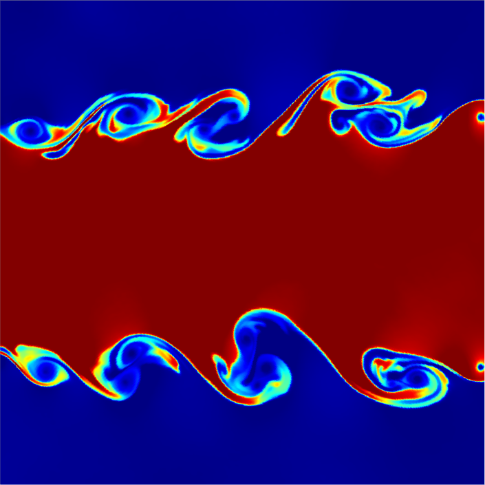
(a) CWENO5

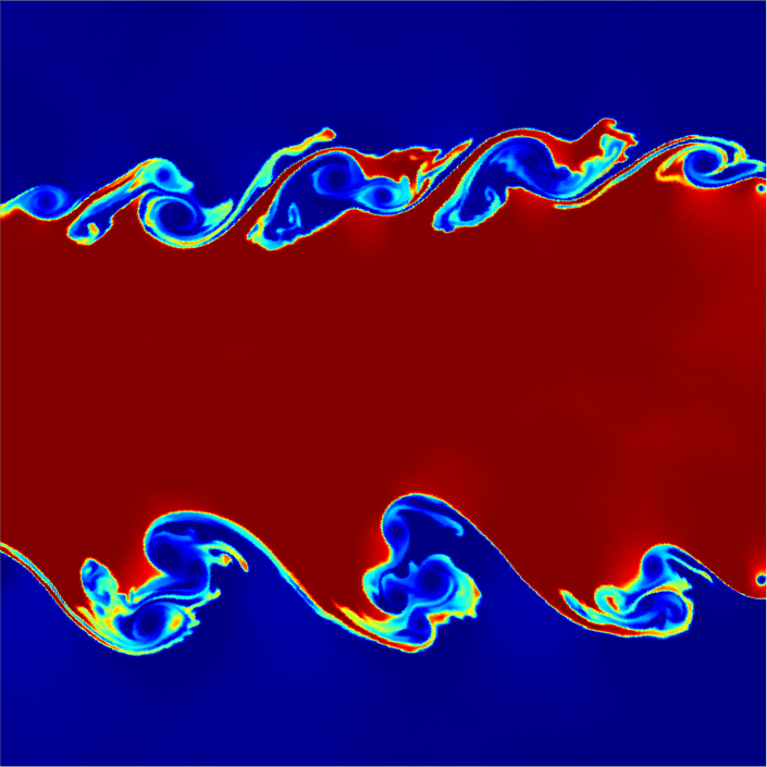
(b) TENO5

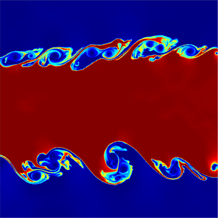
(c) CTENO5

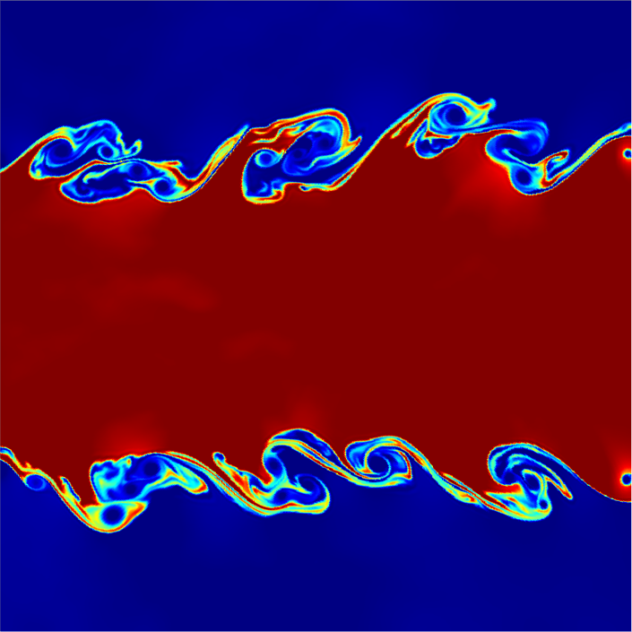
(d) CTENOZ5

(e) CWENO7

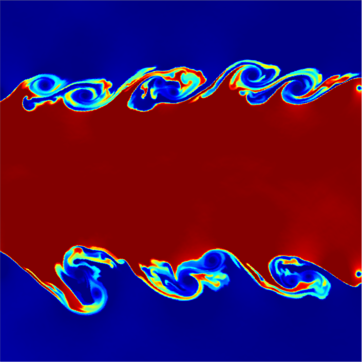
(f) TENO7

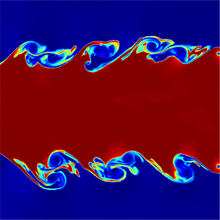
(g) CTENO7

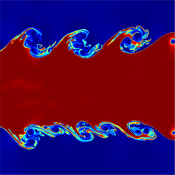
(h) CTENOZ7

Fig. 11: 2D Kelvin-Helmholtz instability: density field from (a)CWENO5, (b)TENO5, (c)CTENO5,(d)CTENOZ5,(e)CWENO7, (f)TENO7, (g)CTENO7,and (h)CTENOZ7. The figures contain 13 density contours ranging from 0.9 to 2.1.

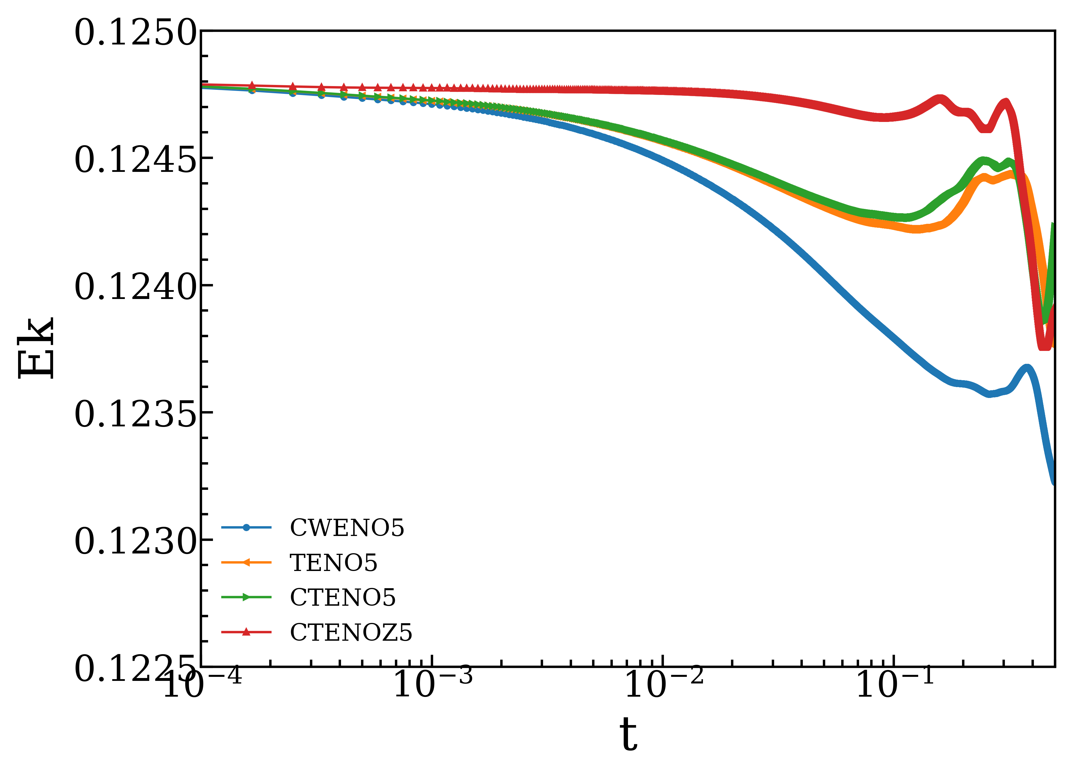
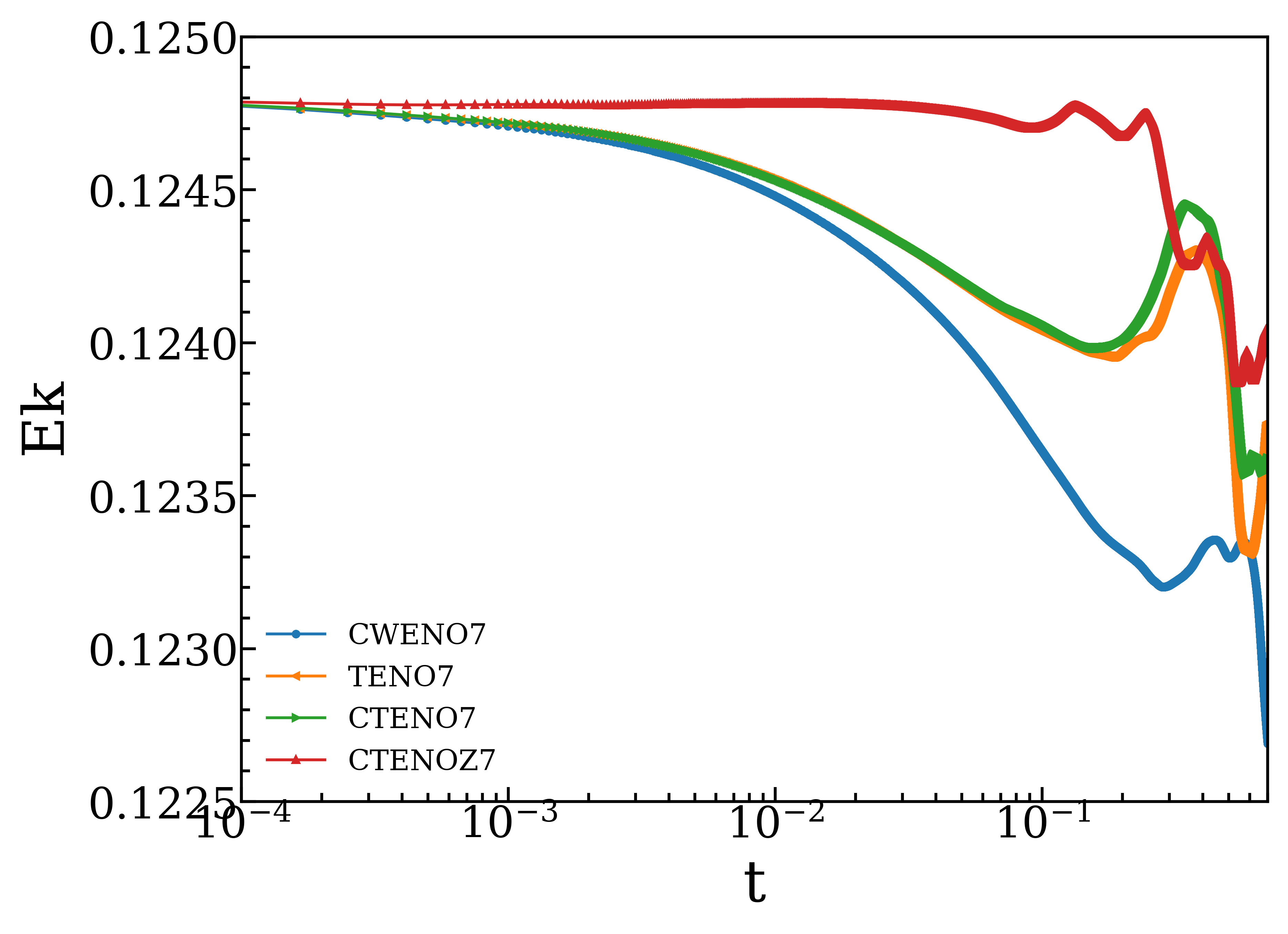
Fig. 12: 2D Kelvin-Helmholtz instability: Time histories of total kinetic energy $E_{K}$ obtained with CWENO, TENO, CTENO,and CTENOZ schemes with 5th and 7th orders.

3.7 Interaction of a Shock Wave with a Wedge in 2D

The Schearldin’s probllem [57], which deals with interaction between shock wave and 2D wedge, is considered in this subsection. The simulation domain we are working with is $[-2,6]\times[-3,3]$, with the wedge tip positioned at $[0,0]$. The length and height of wedge has one unit, with symmetrical conditions imposed on top and bottom regions. The inflow and outflow conditions are assigned to the respective left and right sides. To enhance precision of capturing interaction, unstructured mesh has been refined near the wedge. Fig. 13 visualizes the experimental results at $t=2.1$, utilizing a mesh comprising 413791 uniformly distributed triangular elements. The initial condition is provided according to [58].

$$(\rho,u,v,p)=\begin{cases}(2.122,0.442,0,1.805),\ \text{ if }x<-1\\ (1.4,0,0,1).\ \text{ otherwise }\end{cases}$$ (45)

The density field computed at $t=2.1$ using the CTENO and CTENOZ schemes is presented in Fig. 14, demonstrating well agreement with experimental measurements. Fig. 15 displays shockwave patterns and counter-rotating vortices observed downstream at $t=4$ for different accuracy orders of the proposed CTENO and CTENOZ schemes, exhibiting no visible numerical oscillations in the density fields. These findings indicate that the considered schemes accurately captures all significant flow features in their exact positions, including bow shock, tip vortices, and interface between them.

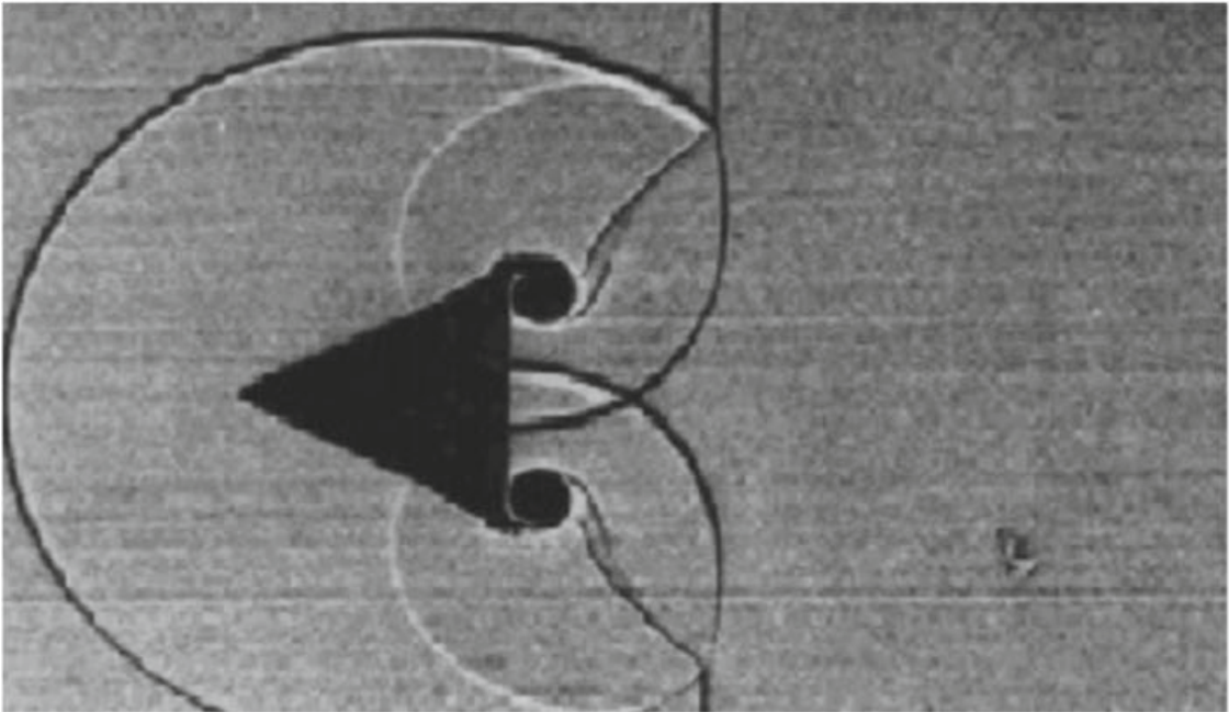
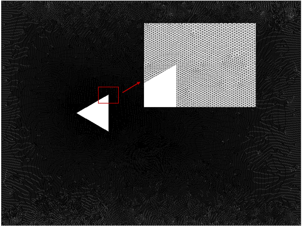
Fig. 13: Interaction of a shock wave with a wedge in 2D: (a) experiment at $t=2.1$ and (b) computational domain with 413791 uniform triangular elements. The region around wedge has being refined.

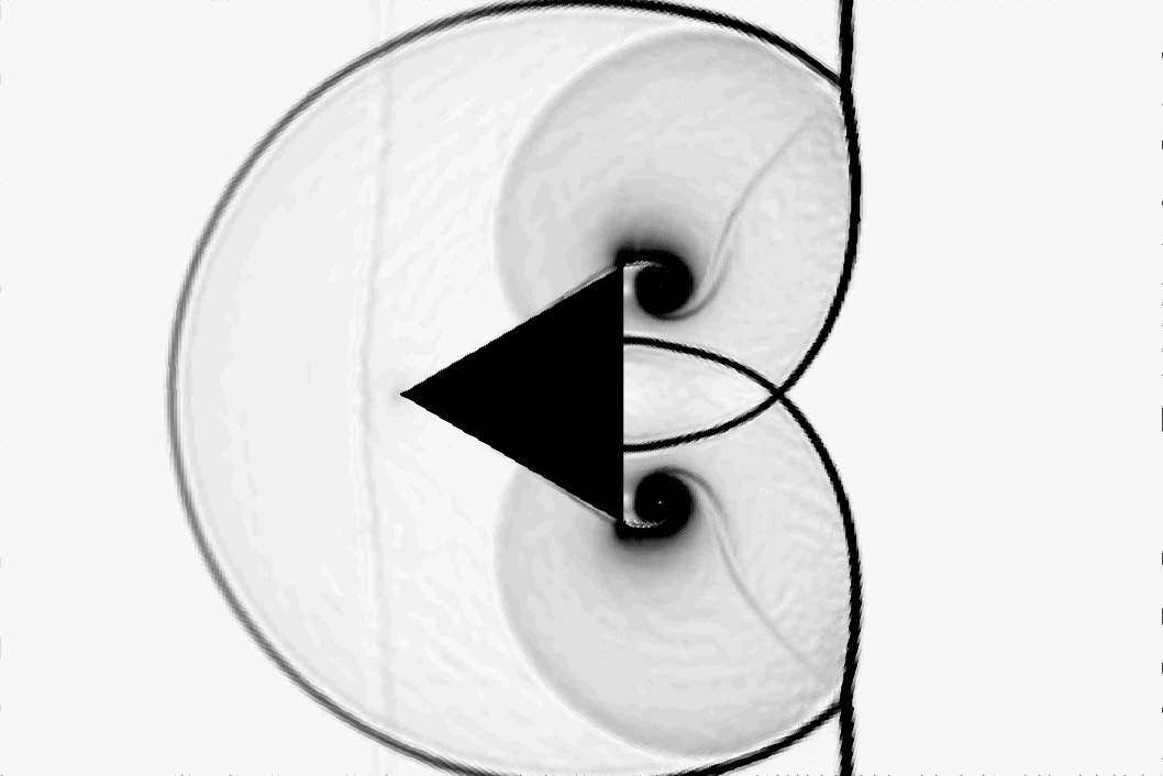
(a) CTENO5

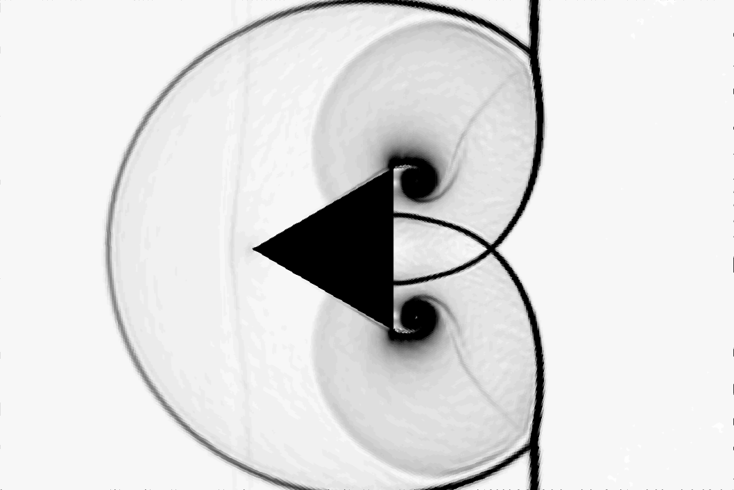
(b) CTENO7

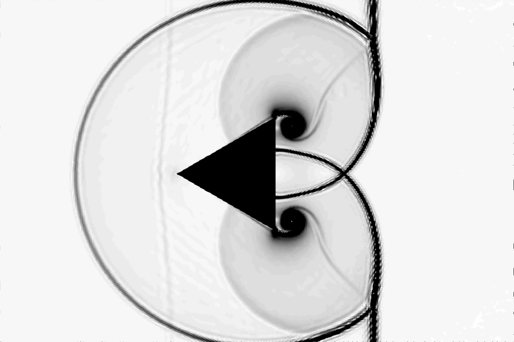
(c) CTENOZ5

(d) CTENOZ7

Fig. 14: Interaction of a shock wave with a wedge in 2D: result from (a)CTENO5,(b)CTENO7,(c)CTENOZ5 and (d)CTENOZ7 scheme at $t=2.1$. The figures contain 40 density gradient magnitude contours ranging from 0 to 5.

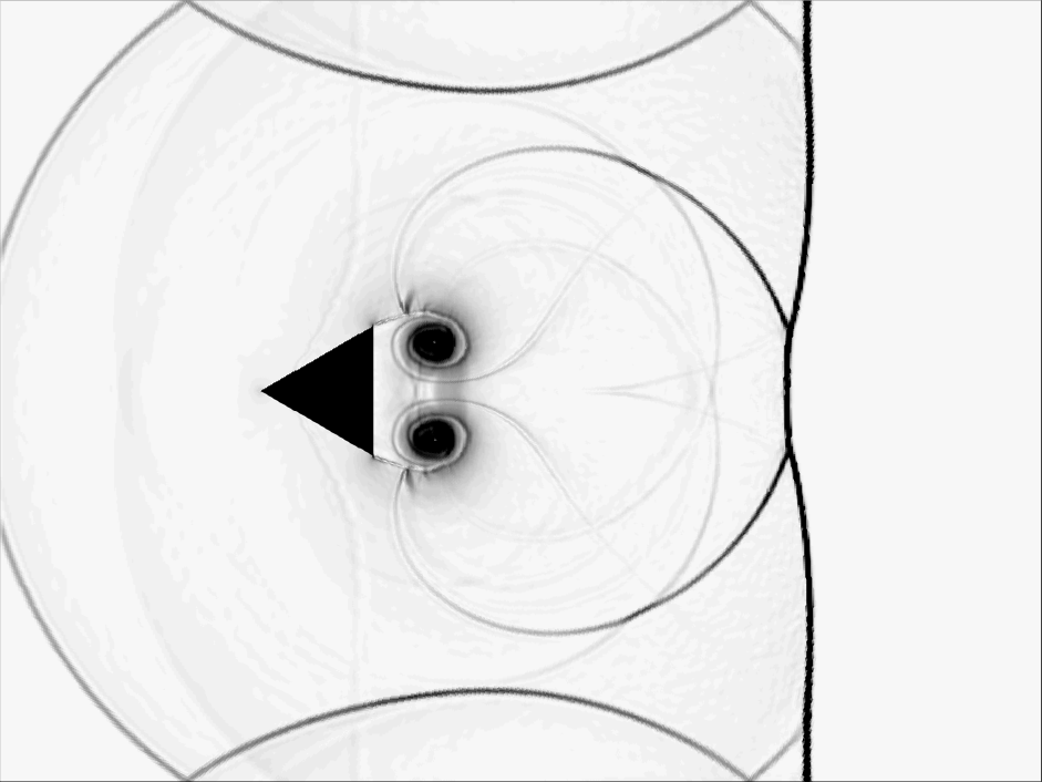
(a) CTENO5

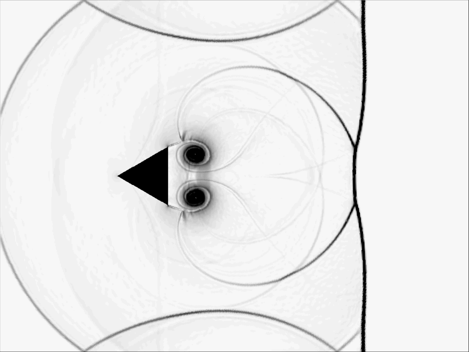
(b) CTENO7

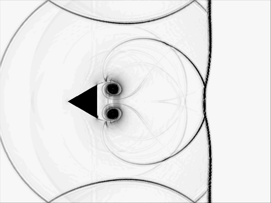
(c) CTENOZ5

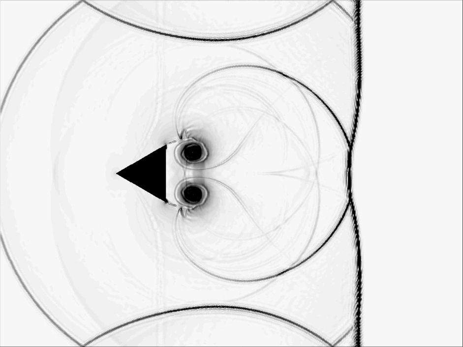
(d) CTENOZ7

Fig. 15: Interaction of a shock wave with a wedge in 2D: result from (a)CTENO5,(b)CTENO7,(c)CTENOZ5,and (d)CTENOZ7 scheme at $t=4$. The figures contain 40 density gradient magnitude contours ranging from 0 to 5.

3.8 Helium Bubble Shock Wave

This model has been created to simulate interaction between bubble and low-intensity shockwave, which is widely utilized to assess numerous methods for modeling multicomponent flow. In this study, quasi-conservative five-equation model is utilized to characterize behavior of inviscid compressible multicomponent flows, which is proposed by Allaire et al. [59]. The equations are closed by incorporating a stiffened gas equation of state. A bubble, consisting of a mixture of helium and air, with a diameter of $D=5cm$, is positioned inside a shock tube filled with air. Bubble is affected by the shockwave traveling from right to left, causing contamination of air. The value of specific heats of air and helium are assigned to values of 1.4 and 1.66 respectively. The initial state is defined in reference [60].

$$\begin{array}[]{c}(a_{1}\rho_{1},a_{2}\rho_{2},u,v,p,a_{1})=\begin{cases}(0.158,0.016,0,0,101325,0.95),\ \text{ for Bubble }\\ (0,1.658,-114.49,0,159060,0),\ \text{ for Post-shock }\\ (0,1.204,0,0,101325,0),\ \text{for Pre-shock }\end{cases}\end{array}$$ (46)

The computational domain utilized in this study is $[-0.25,0.25]\times[0,0.1]$. This domain is composed of three regions, pre-shock, post-shock, and bubble regions.We utilized a unstructured mesh with mixed-element consists of triangular and quadrilateral cells. It is crucial that we refined shock-bubble interaction region to improve the accuracy of our simulations. The total mesh consists of 256252 elements. The slip-wall conditions were imposed at the domain’s top and bottom edges. Inflow and outflow conditions were utilized at right and left edges, respectively. We utilized CTENO and CTENOZ scheme with a 5th-order accuracy, and the simulations were conducted until $t=983\mu s$ with explicit Runge-Kutta method of 3rd-order.

According to the displayed results in Fig. 16, it is clear that CTENO and CTENOZ successfully capture the interaction between the bubble and shockwave during the time evolution. The occurrence of late-stage phenomena, such as the creation of a vortex ring and a jet, has been recognized. These findings align with the qualitative outcomes observed in previous research studies [60, 61]. The instability at the helium bubble interface is amplified by the application of high-order schemes. The spatial-temporal positions of these interfaces reveals a close alignment between the predicted interface positions and the results of reference provided by Terashima and Tryggvason [62] and Quirk and Karni [63].

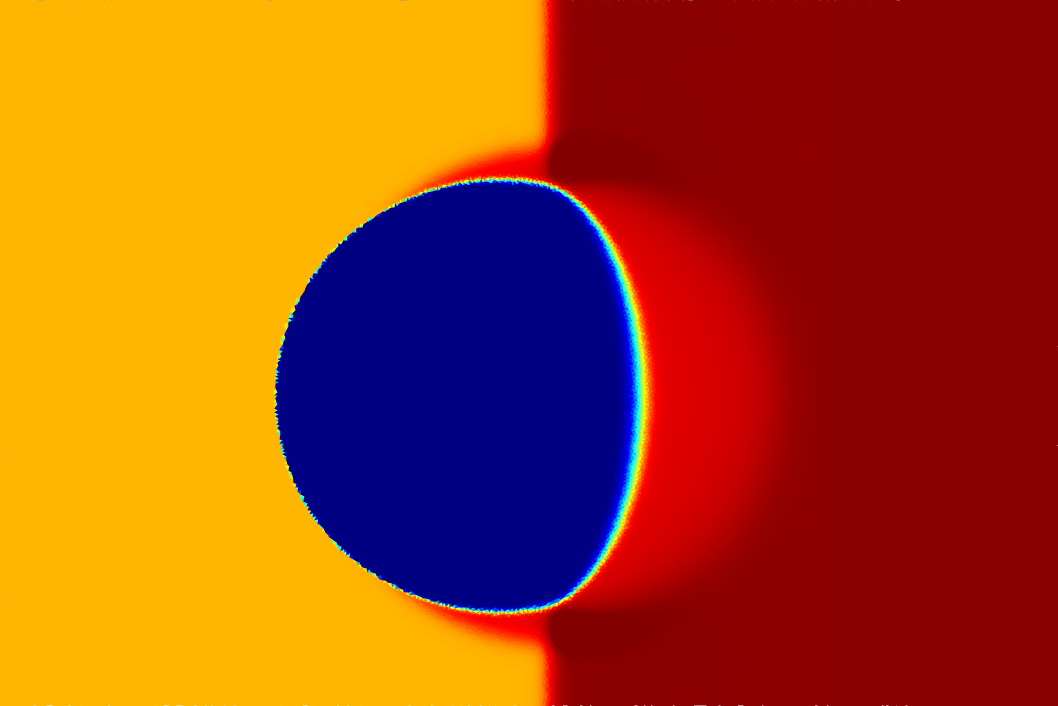
(a) CTENO5 $t=101\mu s$

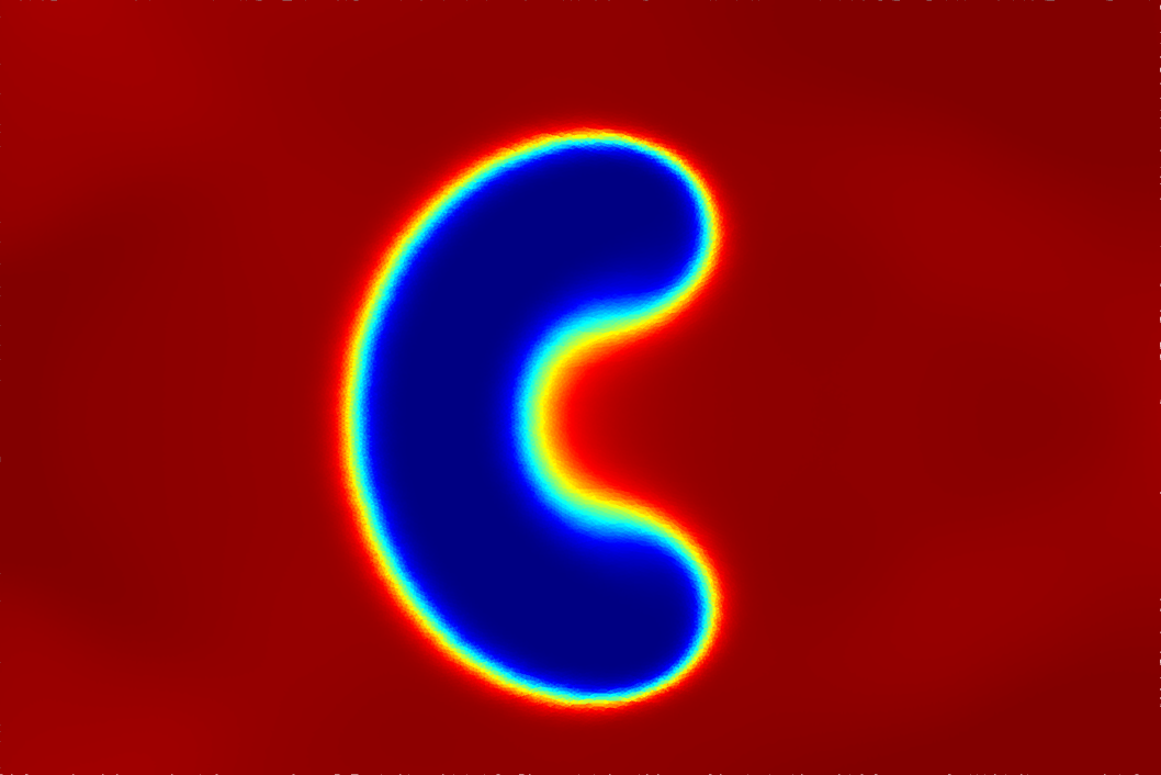
(b) CTENO5 $t=400\mu s$

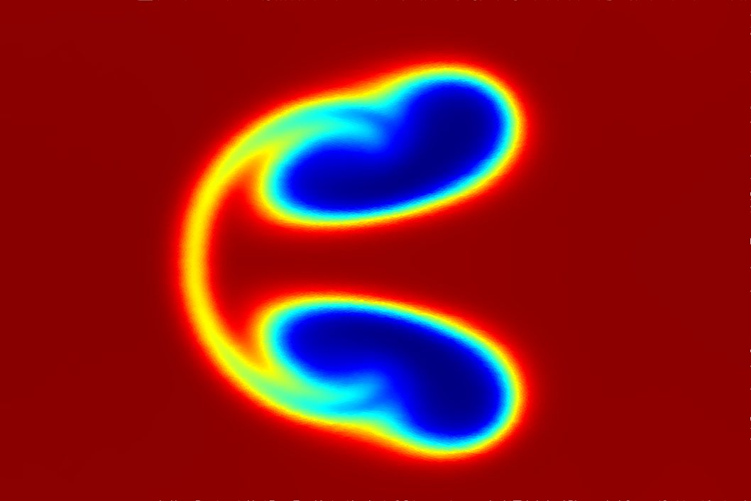
(c) CTENO5 $t=983\mu s$

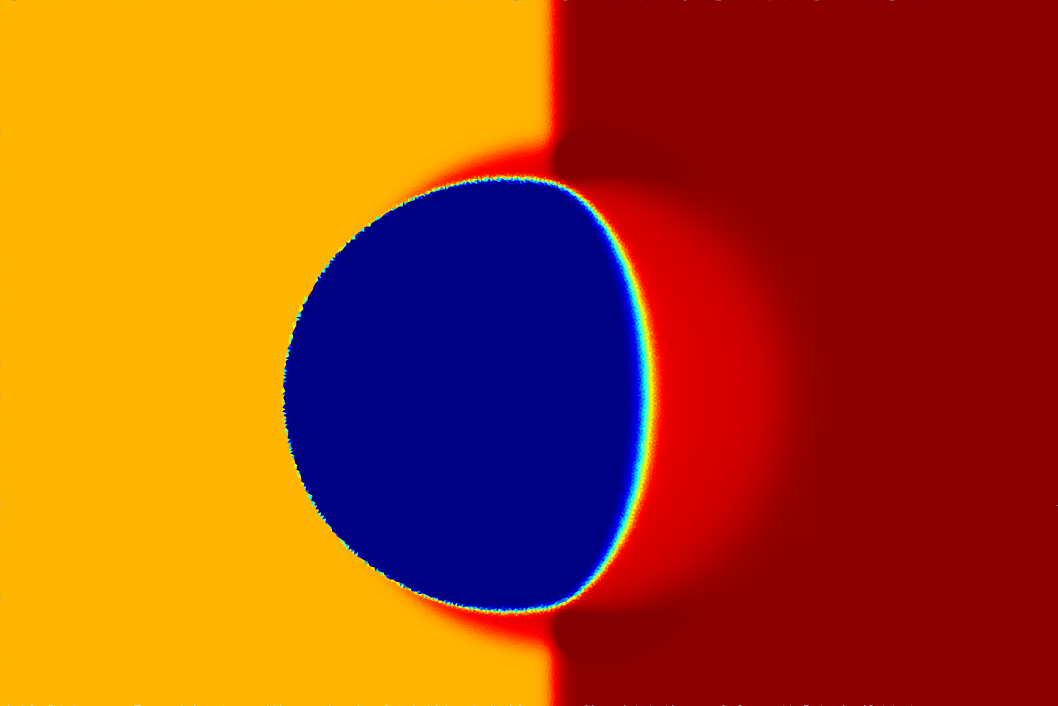
(d) CTENOZ5 $t=101\mu s$

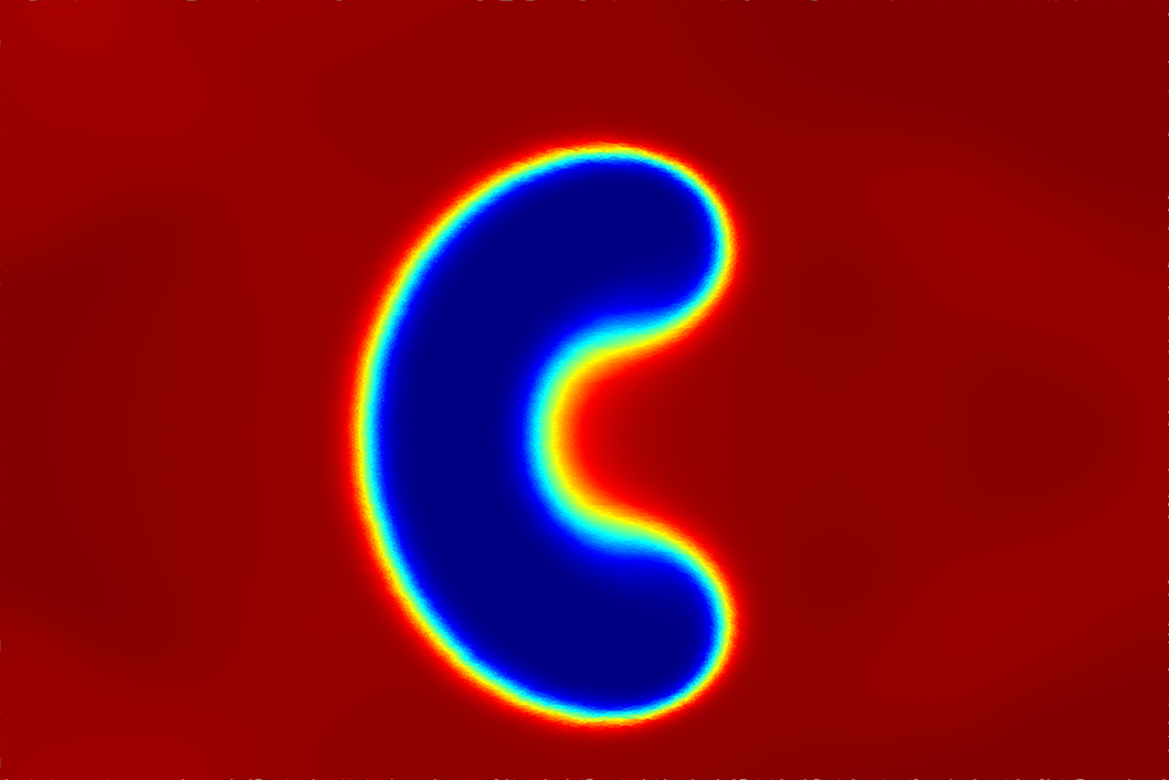
(e) CTENOZ5 $t=400\mu s$

(f) CTENOZ5 $t=983\mu s$

Fig. 16: Helium Bubble Shock Wave:results at various instants from the CTENO and CTENOZ schemes with 5th-order. The figures contain 14 density contours ranging from 0.3 to 1.6.

4 Conclusion

In this study, we expand central targeted ENO family schemes to unstructured meshes with high-order. We have developed and validated a set of CTENO and CTENOZ schemes that exhibit high-order accuracy. These newly proposed schemes are comprised of a stencil with a large central biased and multiple directional small stencils. Compared to WENO candidate stencils with the same order, CWENO, TENO, CTENO, CTENOZ schemes have a more compact overall stencil width. Similar with the TENO used to structured grids, these proposed TENO family schemes in unstructured grids inherit the low-dissipation characteristic by carefully selecting the stencil, optimizing its application, or completely disregarding it when it comes to discontinuities. In order to adapt to unstructured meshes, a ENO-like stencil selection strategy is implemented by employing a rigorous procedure for strong scale separation. The CTENO and CTENOZ weighting strategy guarantees high-order precision by utilizing reconstruction obtained from large central stencil, while preserving ability to accurately capture sharp shocks by choosing candidate reconstruction from small directional stencils. CTENO utilizes optional polynomial and linear coefficients from the CWENO schemes to realise the potential of high order accuracy. After considering smoothness indicators derived from polynomials with varying order of accuracy, CTENOZ schemes exhibits lower dissipation based on CTENO schemes. These schemes are constructed up to the seventh-order accuracy, with its built-in parameters explicitly defined.

Several benchmark simulations were carried out in order to assess the proposed schemes. The numerical findings reveal that these scheme exhibits great robustness in conducting compressible fluid simulations, with low dissipation and ability to accurately capture discontinuities. Moreover, the CTENO and CTENOZ schemes exhibit reduced dissipation and enhanced accuracy compared to CWENO and TENO schemes of equivalent accuracy orders, while still maintaining their strong shock-capturing capability. The parallel scalability is tested in 2D Double Mach Reflection problem, which proves great scaling performance. The computational time of the proposed CTENO and CTENOZ can be roughly equivalent compared to CWENO and TENO schemes, i.e. 2D Double Mach Reflection and Single-Material Triple Point Problem. Considering the impressive effectiveness demonstrated by the CTENO and CTENOZ framework and its potential for future expansion, future research will concentrate on implementing these methods in more complex flows, including chemical-reacting flows and external aerodynamics involving realistic geometries.

References

- [1] Jameson A. Analysis and design of numerical schemes for gas dynamics 1, artificial diffusion, upwind biasing, limiters and their effect on multigrid convergence. riacs technical report no. 94.15. Int J Comput Fluid Dyn, 4(3):171–218, 1995.
- [2] Harten A. High resolution schemes for hyperbolic conservation laws. J Comput Phys, 1983.
- [3] Harten A and Osher S. Uniformly high-order accurate nonoscillatory schemes. SIAM J Numer Anal, 1987.
- [4] Liu X D, Osher S, and Chan T. Weighted essentially non-oscillatory schemes. J Comput Phys, 115(1):200–212, 1994.
- [5] Jiang G S and Shu C W. Efficient implementation of weighted eno schemes. J Comput Phys, 126(1):202–228, 1996.
- [6] Henrick A K, Aslam T D., and Powers J M. Mapped weighted essentially non-oscillatory schemes: Achieving optimal order near critical points. J Comput Phys, 207(2):542–567, 2005.
- [7] Borges R, Carmona M, Costa B, and Don W S. An improved weighted essentially non-oscillatory scheme for hyperbolic conservation laws. J Comput Phys, 227(6):3191–3211, 2008.
- [8] Johnsen E, Larsson J, Bhagatwala A V., Cabot W H., Moin P, Olson B J., Rawat P S., Shankar S K., S.Green B.Rn, and Yee H C. Assessment of high-resolution methods for numerical simulations of compressible turbulence with shock waves. J Comput Phys, 229(4):1213–1237, 2010.
- [9] Acker F., De R. Borges R B., and Costa B. An improved weno-z scheme. J Comput Phys, pages 726–753, 2016.
- [10] Hill D J and Pullin D I. Hybrid tuned center-difference-weno method for large eddy simulations in the presence of strong shocks. J Comput Phys, 194(2):435–450, 2004.
- [11] Weirs V G. and Candler G. Optimization of weighted eno schemes for dns of compressible turbulence. In 13th Computational Fluid Dynamics Conference, 1997.
- [12] Yan Z G, Liu H Y, Mao M L, Zhu H J, and Deng X G. New nonlinear weights for improving accuracy and resolution of weighted compact nonlinear scheme. Comput & Fluids, 127:226–240, 2016.
- [13] Shu C W. Essentially non-oscillatory and weighted essentially non-oscillatory schemes. Acta Numer, 29:701–762, 2020.
- [14] Fu L, Hu X Y, and Adams N A. A family of high-order targeted eno schemes for compressible-fluid simulations. J Comput Phys, 305, 2016.
- [15] Fu L. A low-dissipation finite-volume method based on a new teno shock-capturing scheme. Comput Phys Comm, 235:25–39, 2019.
- [16] Ye C C, P J Y Zhang, Wan Z H, and Sun D J. An alternative formulation of targeted eno scheme for hyperbolic conservation laws. Comput & Fluids, (238-), 2022.
- [17] Haimovich O and Frankel S H. Numerical simulations of compressible multicomponent and multiphase flow using a high-order targeted eno (teno) finite-volume method. Comput & Fluids, 146:105–116, 2017.
- [18] Dong H, Fu L, Zhang F, Liu Y, and Liu J. Detonation simulations with a fifth-order teno scheme. Commun. Comput. Phys., 25(5):1357–1393, 2019.
- [19] Lusher D J. and Sandham N D. Shock-wave/boundary-layer interactions in transitional rectangular duct flows. Appl Sci Res, 105(6), 2020.
- [20] Lusher D J. and Sandham N. Assessment of low-dissipative shock-capturing schemes for transitional and turbulent shock interactions. In AIAA Aviation 2019 Forum, 2019.
- [21] Vincent P. E. and Jameson A. Facilitating the adoption of unstructured high-order methods amongst a wider community of fluid dynamicists. Math Model Nat Phenom, 6(3):97–140, 2011.
- [22] Hu C and Shu C W. Weighted essentially non-oscillatory schemes on triangular meshes. J Comput Phys, 150(1):97–127, 1999.
- [23] Zhang Y T and Shu C W. Third order weno scheme on three dimensional tetrahedral meshes. Commun Comput Phys, 5(2):836–848, 2009.
- [24] Shi J, Hu C, and Shu C W. A technique of treating negative weights in weno schemes. J Comput Phys, 175(1):108–127, 2002.
- [25] Zhu J and Shu C W. A new type of multi-resolution weno schemes with increasingly higher order of accuracy on triangular meshes. J Comput Phys, 2019.
- [26] B Dinshaw S Balsara A. An efficient class of weno schemes with adaptive order for unstructured meshes - sciencedirect. J Comput Phys, 404, 2019.
- [27] Michael D and Martin K. Arbitrary high order non-oscillatory finite volume schemes on unstructured meshes for linear hyperbolic systems. J Comput Phys, 221(2):693–723, 2007.
- [28] Levy D. Compact central weno schemes for multidimensional conservation laws. SIAM J, 2000.
- [29] Dumbser M, Boscheri W, Semplice M, and Russo G. Central weighted eno schemes for hyperbolic conservation laws on fixed and moving unstructured meshes. SIAM J Sci Comput, 39(6):A2564–A2591, 2017.
- [30] Panagiotis T and Michael D. Arbitrary high order central non-oscillatory schemes on mixed-element unstructured meshes. Comput & Fluids, 2021.
- [31] Panagiotis T, Adebayo E M, Merino A C, Arjona A P, and Skote M. Cweno finite-volume interface capturing schemes for multicomponent flows using unstructured meshes. J Sci Comput, (3), 2021.
- [32] Ji Z, Liang T, and Fu L. A class of new high-order finite-volume teno schemes for hyperbolic conservation laws with unstructured meshes. J Sci Comput, 92(2):1–39, 2022.
- [33] Ji Z, Liang T, and Fu L. High-order finite-volume teno schemes with dual eno-like stencil selection for unstructured meshes. J Sci Comput, 95(3), 2023.
- [34] Panagiotis T. Stencil selection algorithms for weno schemes on unstructured meshes. J Comput Phys, 2019.
- [35] Antonis F. A, Dimitris D, Pericles S. F, Fu L, Ioannis K, Xesús N, Paulo A.S.F. Silva, Martin S, Vladimir T, and Panagiotis T. Ucns3d: An open-source high-order finite-volume unstructured cfd solver. Comput Phys Commun, 279:108453, 2022.
- [36] George K and Vipin K. Multilevelk-way partitioning scheme for irregular graphs. J PARALLEL DISTR COM, 48(1):96–129, 1998.
- [37] Panagiotis T, Antonis F A, and Karl W J. Improvement of the computational performance of a parallel unstructured weno finite volume cfd code for implicit large eddy simulation. Comput & Fluids, 173:157–170, 2018.
- [38] Bartosz D W, Freddie D W, Francis P R, Vincent P E, and Paul H J K. Gimmik—generating bespoke matrix multiplication kernels for accelerators: Application to high-order computational fluid dynamics. Comput Phys Commun, 202:12–22, 2016.
- [39] Loppi N A, Witherden F D, Jameson A, and Vincent P E. A high-order cross-platform incompressible navier–stokes solver via artificial compressibility with application to a turbulent jet. Comput Phys Commun, 233:193–205, 2018.
- [40] Panagiotis T, Antoniadis A F, and Drikakis D. Weno schemes on arbitrary unstructured meshes for laminar, transitional and turbulent flows. J Comput Phys, 256(1):254–276, 2014.
- [41] Gottlieb S and Shu C W. Total variation diminishing runge-kutta schemes. Math Comp, 67(221), 1996.
- [42] Drikakis A D. Weno schemes on arbitrary unstructured meshes for laminar, transitional and turbulent flows. J Comput Phys, 2014.
- [43] Stewart G W. Matrix algorithms: basic decompositions. Soc Ind App, 1998.
- [44] Fu L. A very-high-order teno scheme for all-speed gas dynamics and turbulence. Comput Phys Commun, 244:117–131, 2019.
- [45] Fu L, Hu X Y., and Adams N A. A new class of adaptive high-order targeted eno schemes for hyperbolic conservation laws. J Comput Phys, 374:S0021999118305047–, 2018.
- [46] Fu L, Hu X Y., and Adams N A. Targeted eno schemes with tailored resolution property for hyperbolic conservation laws. J Comput Phys, pages 97–121, 2017.
- [47] Castro M, Costa B, and Don W. High order weighted essentially non-oscillatory weno-z schemes for hyperbolic conservation laws. J Comput Phys, 230(5):1766–1792, 2011.
- [48] Zhu J and Qiu J. New finite volume weighted essentially nonoscillatory schemes on triangular meshes. SIAM J Sci Comput, 2018.
- [49] Zhu J and Shu C W. A new type of third-order finite volume multi-resolution weno schemes on tetrahedral meshes. J Comput Phys, 406(6):109212, 2019.
- [50] Toro E. F., Spruce M., and Speares W. Restoration of the contact surface in the hll-riemann solver. Shock Waves, 4(1):25–34, 1994.
- [51] Sod Gary A. A survey of several finite difference methods for systems of nonlinear hyperbolic conservation laws. J Comput Phys, 27(1):1–31, 1978.
- [52] Shu C W and Osher S. Efficient implementation of essentially non-oscillatory shock-capturing schemes. J Comput Phys, 77(2):439–471, 1989.
- [53] Paul W and Phillip C. The numerical simulation of two-dimensional fluid flow with strong shocks. J Comput Phys, 54(1):115–173, 1984.
- [54] Panagiotis T. Extended bounds limiter for high-order finite-volume schemes on unstructured meshes. J Comput Phys, page S0021999118300858, 2018.
- [55] Zeng X. and Scovazzi G. A frame-invariant vector limiter for flux corrected nodal remap in arbitrary lagrangian–eulerian flow computations. J Comput Phys, 270(3):753–783, 2014.
- [56] San O and Kara K. Evaluation of riemann flux solvers for weno reconstruction schemes: Kelvin–helmholtz instability. Comput & Fluids, 117:24–41, 2015.
- [57] Milton, Van, Dyke, Editor, Frank, M., White, and Reviewer. An album of fluid motion. J Fluids Eng, 1982.
- [58] Dumbser M, KSer M, Titarev V A., and Toro E F. Quadrature-free non-oscillatory finite volume schemes on unstructured meshes for nonlinear hyperbolic systems. J Comput Phys, 226(1):204–243, 2007.
- [59] Grégoire A, Sébastien C, and Kokh S. A five-equation model for the simulation of interfaces between compressible fluids. J Comput Phys, 181(2):577–616, 2002.
- [60] Sturtevant B. and Haas J. F. Interaction of weak shock waves with cylindrical and spheric inhomogeneities. 1987.
- [61] Vedran C and Tim C. Finite-volume weno scheme for viscous compressible multicomponent flows. J Comput Phys, 274:95–121, 2014.
- [62] Hiroshi T and Grétar T. A front-tracking/ghost-fluid method for fluid interfaces in compressible flows. J Comput Phys, 228(11):4012–4037, 2009.
- [63] Quirk J J. and Karni S. On the dynamics of a shock–bubble interaction. J Fluid Mech, 318:129–163, 1996.