Quantum Liquid: From the perspective of Surface Tension

Abstract

We analyze the surface tension in ultra-cold atomic gases in quasi one dimensional and one dimensional geometry. In recent years, experimental observations have confirmed the “clustering of atoms” to form droplets in ultra-cold atomic gases and the emergence of this new phase is attributed to the beyond mean-field interaction. However, two decades earlier, liquid formation was predicted due to the competition of two-body and three-body interactions. Here, we review both the propositions and comment on the role of beyond mean-field and three-body interaction in liquid formation by calculating the surface tension.

I Introduction

The physics at ultra-low temperature is always a matter of extreme interest. In this direction a new impetus has been provided through the experimental observations of liquid-like phase in ultra-cold gases Kadau et al. (2016); Li et al. (2017); Cabrera et al. (2018); Chomaz et al. (2019); Böttcher et al. (2019); Tanzi et al. (2019); Donner (2019). The experimental observation is treated as verification of the suggested theoretical framework offered recently Petrov (2015); Petrov and Astrakharchik (2016). In the current theoretical model, the beyond mean-field (BMF) contribution (proposed by Lee-Huan-Yang Lee et al. (1957)) is considered as the catalyst in the stabilization mechanism which in effect supports the formation of the liquid-like droplets (can be called as dropleton). One of the prominent signatures of the formation of liquid-like states is the homogeneous spatial density Ferrier-Barbut (2019).

However, one must note that, about two decades ago, a similar state of matter was predicted based on the Efimov effect which results in creation of three-body bound states Bulgac (2002); Bedaque et al. (2003); Bulgac (2020). The competition between the two-body mean-field interaction (cubic non-linearity) and three-body interaction (quintic non-linearity) is at the heart of this theory. The liquid formation was substantiated through the calculation of non-zero surface tension.

In recent years there have been some suggestions that the flat-top density distribution arising from the competition between cubic-quintic non-linearity, actually points to flat-top solitons (FTS) or platicons which are different from the droplets in its dynamical nature Lobanov et al. (2021); Alotaibi et al. (2023). In this context, we plan to investigate the ambiguity associated with dropleton and platicon by analyzing the non-linear Schrodinger equation with LHY correction and three-body interaction (as suggested in Ref.Bulgac (2002)) in one dimensional (1D) and quasi 1D (Q1D) systems.

The theoretical discussions on droplet formation in 1D Bose gas or in a Q1D binary Bose-Einstein condensate (BEC) revolves around the nature of the BMF interaction. To be more precise, in the 1D system the BMF interaction manifests via quadratic non-linearity Petrov and Astrakharchik (2016); Astrakharchik and Malomed (2018) while it is quartic non-linearity in Q1D Debnath and Khan (2021). Our primary objective is to study the competition between two-body mean-field interaction, BMF and three-body interaction in liquid formation. For this purpose, we will rely on the calculation of surface tension.

We have arranged our results in the following way: in Sec. II we summarize the recent theoretical model to describe Q1D and 1D systems after taking into account the LHY contribution. Later, we note down the equation of motion in Q1D and 1D with three-body interaction, which we describe as cubic-quartic-quintic non-linear Schrödinger equation (CQQNLSE) and quadratic-cubic-quintic non-linear Schrödinger equqaiton (QCQNLSE) respectively. In the next section i.e., in Sec.III we explicate the analytical solutions and calculate the surface tension. Our findings relate to both the dimensions and we identify the role of interaction as well as dimensionality in liquid formation. We draw our conclusion in Sec.IV.

II Theoretical Models

In this section we plan to summarize the existing theories for both Q1D and 1D. The theory of Q1D is derived from the three dimensional model Petrov (2015) with suitable dimension reduction technique (which we will touch upon here) Debnath and Khan (2021) and the 1D theory is provided in Ref. Petrov and Astrakharchik (2016).

Quasi-One-Dimensional System

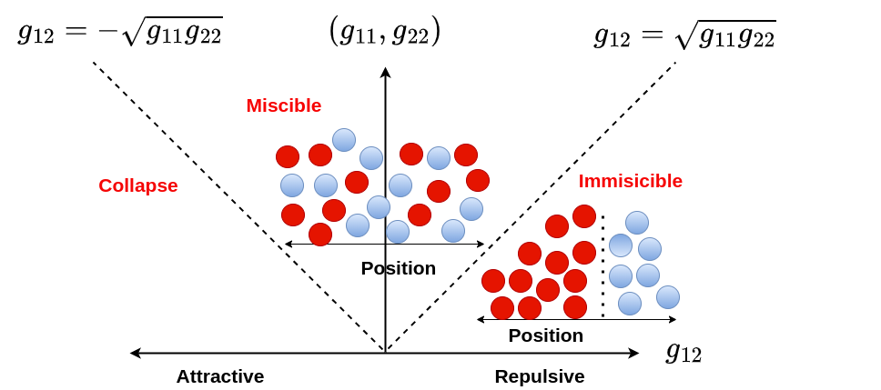
Figure 1: Schematic representation of the competition between inter-species and intra-species interactions in atomic two component BEC and associated quantum states. The red and blue circles represent two different atomic species.

In two-component BEC or binary BEC (the two components can be two different species of atoms Pu and Bigelow (1998) or two-different hyper-fine states of same species Myatt et al. (1997)) due to the competition between inter-species and intra-species interactions one can observe distinct mixing dynamics (as schematically described in Fig. 1). The intra-species coupling is described via $g_{11}$ and $g_{22}$ while the inter-species interaction is denoted as $g_{12}$. If $g_{11},g_{22}$ and $g_{12}$ all are repulsive then we can look forward to transition between miscible and the immiscible phase. The condensate will be in miscible phase when $-\sqrt{g_{11}g_{22}}<g_{12}<\sqrt{g_{11}<g_{22}}$, and will be in immiscible phase when $g_{12}>\sqrt{g_{11}g_{22}}$ while the condensate will collapse for $-\sqrt{g_{11}g_{22}}>g_{12}$.

In a uniform Bose mixture, having two components of masses $m_{1}$ and $m_{2}$ Ancilotto et al. (2018), the coupling constant of intra-species($g_{11}=4\pi a_{11}\hbar^{2}/m_{1},\hskip 5.69054ptg_{22}=4\pi a_{22}\hbar^{2}/m_{2}$) and inter-species($g_{12}=2\pi a_{12}\hbar^{2}/m_{r}$) interactions, where $m_{r}$ is the reduced mass ($m_{1}m_{2}/(m_{1}+m_{2}$) and, $a_{11}$ and $a_{22}$ are the intra-species interaction, both are positive, meanwhile inter-species $a_{12}$ is negative. If number densities are $n_{1}$ and $n_{2}$ then there normalized form can be represented respectively as : $\int_{V}n_{1}dr=N_{1}$ and $\int_{V}n_{2}dr=N_{2}$. Here, $N=N_{1}+N_{2}$ represents the total number of bosons in the mixture along with the total number density, $n=n_{1}+n_{2}$. Therefore, energy functional can be written as Cappellaro et al. (2018),

$$E = \sum_{j=1,2}\Big{[}\frac{\hbar^{2}}{2m}|\nabla\psi_{j}|^{2}+V_{ex}(r)|\psi_{j}|^{2}+\frac{1}{2}g_{jj}|\psi_{j}|^{4}\Big{]}$$ (1)

$$+g_{12}|\psi_{1}|^{2}|\psi_{2}|^{2}+E_{BMF}(\psi_{1},\psi_{2}).$$

Here, $E_{BMF}$ stands for the beyond mean-field interaction energy. As described in Fig. 1, near the line of collapse where the effective interaction $g_{12}+\sqrt{g_{11}g_{22}}\rightarrow 0$, the relatively weak BMF interaction plays important role in stabilizing the system. For the case when we had gone close to the MF instability boundary i.e $\delta g<0$, we need to avoid the imaginary contribution for which we approximate that the instability is very weak i.e $|\delta g|<<g$ and hence we assume $|\delta g|\approx 0$.

Now, considering that density ratio will be $n_{1}/n_{2}=\sqrt{g_{22}/g_{11}}$ = $\eta$, via two components have indistinguishable spatial mode $n_{i=1,2}=|\psi|^{2}$. Therefore, $g$ = $\sqrt{g_{11}g_{22}}$ and $\delta g$ = $g+\sqrt{g_{11}g_{22}}$. The energy functional in Eq.(1) can now be rewritten as,

$$E = \frac{\hbar^{2}}{2m}|\nabla\psi|^{2}+V_{trap}|\psi|^{2}+\delta g\frac{\eta}{(\eta+1)^{2}}|\psi|^{4}$$ (2)

$$+\frac{8m^{3/2}}{15\pi^{2}\hbar^{3}}(\eta g_{11})^{5/2}|\psi|^{5}$$

The corresponding effective one component equation of motion can be noted as Cheiney et al. (2018),

$$i\hbar\frac{\partial\psi}{\partial t}=\Big{[}-\frac{\hbar^{2}}{2m}\nabla^{2}+V_{trap}+U|\psi|^{2}+U^{{}^{\prime}}|\psi|^{3}\Big{]}\psi,$$ (3)

where, $U$ = $2\delta g\frac{\eta}{(1+\eta)^{2}}n$ and $U^{{}^{\prime}}$ = $\frac{4m^{3/2}}{3\pi^{2}\hbar^{3}}(ng_{11})^{5/2}n^{3/2}$. Here, it is important to note that the above equation contains two types of non-linearity: one is cubic non-linearity, which is responsible for the mean field (MF) interaction and another is quartic non-linearity which is justification of beyond mean field (BMF) interaction.

In Eq.(3), the external potential $V_{trap}$ has two components: one in the transverse direction, defined as $V_{T}(y,z)=\frac{1}{2}m\omega^{2}_{\perp}(y^{2}+z^{2})$ and the other in the longitudinal direction, noted as $V_{L}(x)=\frac{1}{2}m\omega_{o}^{2}x^{2}$ where $\omega_{\perp}$ and $\omega_{o}$ is the transverse and longitudinal trap frequency respectively Khaykovich et al. (2002). One can now conveniently reduce Eq.(3) from $3+1$ dimension to $1+1$ dimension by setting $\omega_{\perp}$ as ten times the $\omega_{o}$. Hence, by tuning the trapping frequency it is possible to create a cigar shaped BEC in quasi one dimension. For a trapped gas the characteristic length scale is defined as $a_{\perp}=\sqrt{\frac{\hbar}{m\omega_{\perp}}}$, however, in quasi one dimension it would be, $a_{x}/a_{\perp}\approx\sqrt{10}$. Here, $a_{x}$ will be $a_{x}=\sqrt{\frac{\hbar}{m\omega_{o}}}$. In order to reduce the dimension of Eq.(3) in an effective one dimensional (Q1D) equation we consider an ansatz of the following form Khan and Panigrahi (2013),

$$\psi(r,t)=\frac{1}{\sqrt{2\pi a_{B}a_{\perp}}}\psi\Big{(}\frac{x}{a_{\perp}},\omega_{\perp}t\Big{)}e^{\Big{(}-i\omega_{\perp}t-\frac{y^{2}+z^{2}}{a_{\perp}^{2}}\Big{)}}$$ (4)

A systematic and careful calculation then leads to the Q1D CQNLSE (here, we have ignored the details for brevity),

$$i\frac{\partial\psi(r,t)}{\partial t} = \left[-\frac{1}{2}\frac{\partial^{2}\psi(x,t)}{\partial x^{2}}+\frac{1}{2}Kx^{2}+G_{1}|\psi(x,t)|^{2}\right.$$ (5)

$$\left.+G_{4}|\psi(x,t)|^{3}\right]\psi(x,t),$$

where $G_{1}=\frac{\delta gnm}{4\pi a_{B}\hbar^{2}}$, $G_{4}=\frac{\sqrt{2}}{3}\frac{m^{3/2}n^{3/2}g_{sym}^{5/2}}{\pi^{2}a_{B}^{3/2}a_{\perp}\hbar^{5}}$, $g_{sym}=g_{11}=g_{22}$ and $K={\omega_{o}^{2}}/{\omega_{\perp}^{2}}$. In a more generic manner we can write the equation as,

$$i\frac{\partial\psi(r,t)}{\partial t} = \left[-\frac{1}{2}\frac{\partial^{2}\psi(x,t)}{\partial x^{2}}+V(x)+g_{1}|\psi(x,t)|^{2}\right.$$ (6)

$$\left.+g_{4}|\psi(x,t)|^{3}\right]\psi(x,t),$$

Here, $g_{1}$ and $g_{4}$ stands for the MF and BMF interaction strength while $V(x)$ is the external potential.

One Dimensional System

Contrary to the Q1D picture (derived from three dimensional setup), in 1D Bose gas the BMF contribution manifests as quadratic non-linearity. Further, one can also note that the nature of MF and BMF interaction is reversed in 1D, i.e., MF interaction is repulsive and BMF interaction is attractive.

In 1D system, we define, $\delta g$ = $g_{12}+\sqrt{g_{11}g_{22}}$ which is in the vicinity of unstable region which implies $0<\delta g<\sqrt{g_{11}g_{22}}$. Therefore, to explain the one dimension GP equation including the beyond mean field (BMF) correction, a small variation between the inter-component attraction strength $(g_{12<0})$ and intra-component self-repulsion, $\delta g=g+g_{12}>0$ along with $g<0$, can be expressed as Debnath et al. (2022),

$$i\hbar\frac{\partial\psi}{\partial t}=-\frac{\hbar^{2}}{2m}\frac{\partial^{2}\psi}{\partial x^{2}}+V(x)\psi+\delta g|\psi|^{2}\psi-\frac{\sqrt{2m}}{\pi\hbar}g^{3/2}|\psi|\psi,$$ (7)

where $V(x)$ is the external potential and $m$ is the atomic mass. For further analysis we write the equation motion in a more generic form such that,

$$i\frac{\partial\psi}{\partial t}=-\frac{1}{2}\frac{\partial^{2}\psi}{\partial x^{2}}+V(x)\psi+g_{3}|\psi|^{2}\psi+g_{2}|\psi|\psi.$$ (8)

Here, $g_{3}$ and $g_{2}$ denote the strength of the MF and BMF interactions respectively.

Inclusion of Three-Body Interaction

In the earlier subsections, we have discussed the inclusion of BMF contribution in the GP equation at lower dimensions. However, exactly two decades ago, we found the first suggestion of droplet formation due to the competition between two-body MF interaction and three-body interaction Bulgac (2002); Bedaque et al. (2003); Bulgac (2020). Here, we plan to explicate the formalism introduced in Ref. Bulgac (2002).

It is well known that, for a dilute Bose system if two-body scattering length is very large i.e., $a>>r_{0}$, where $r_{0}$ is the range of the potential, we start observing three-body bound state formation. This is commonly described as the Efimov effect Efimov (1973). In this regime there are two independent dimensionless parameters $\rho a^{3}$ and $\rho r_{0}^{3}$. The three-body bound states appear irrespective of whether the two-body scattering length is positive or negative. It is further noted that, if the three-body zero-energy scattering amplitude defined as $g_{3}$ then the contribution of the three-particle collisions to the ground state energy density of a dilute Bose gas can be expressed as, $\mathcal{E}_{3}(\rho)=\frac{1}{6}g_{3}\rho^{3}$. In this situation, the ground state energy for N bosons in an ensemble can be noted as,

$$E(N)=\int d^{3}r\Big{[}\frac{\hbar^{2}}{2m}|\nabla\psi(r)|^{2}+\frac{1}{2}g_{1}\rho(r)^{2}+\frac{1}{6}g_{3}\rho(r)^{3}\Big{]}$$ (9)

Here, $\rho(r)=|\psi(r)|^{2}$ is the number density. Also $g_{1}={4\pi\hbar^{2}a}/{m}$ ($a$ = two particle scattering length and $m$ = particle mass).

Following the usual prescription of energy minimization and applying the dimensional reduction method expressed in earlier, we can write the equation of motion as,

$$i\hbar\frac{\partial\psi}{\partial t}=-\frac{\hbar^{2}}{2m}\frac{\partial^{2}\psi}{\partial x^{2}}+\frac{g_{1}}{2}|\psi|^{2}\psi+\frac{g_{3}}{6}|\psi|^{4}\psi$$ (10)

However, accounting the result from Eq. 6 and Eq. 8 and incorporating the three-body interaction in these equations the effective cubic-quartic-quintic NLSE (CQQNLSE) and quadratin-cubic-quintic NLSE (QCQNLSE) will read:

$$i\frac{\partial\psi}{\partial t} = -\frac{1}{2}\frac{\partial^{2}\psi}{\partial x^{2}}+g_{1}|\psi|^{2}\psi+g_{4}|\psi|^{3}\psi$$ (11)

$$+g_{3}|\psi|^{4}\psi+V(x)\psi$$

$$i\frac{\partial\psi}{\partial t} = -\frac{1}{2}\frac{\partial^{2}\psi}{\partial x^{2}}+g_{1}|\psi|^{2}\psi+g_{2}|\psi|\psi$$ (12)

$$+g_{3}|\psi|^{4}\psi+V(x)\psi$$

where, $g_{1}$ and $g_{3}$ are the two-body and three body interaction strength respectively. $g_{2}(g_{4})$ describes the BMF interaction in 1D (Q1D) geometry while $V(x)$ stands for external potential. In the next section we will propose the possible analytical solution. Further, we will comment on the potential structures which are essential to stabilize the solutions. Also in the above equations, we have not made any specific comment on the nature of the interactions which we plan to explicate in the next section.

III Analytical solutions

In the preceding section we have discussed the equation of motion in different geometries and explicated the intriguing nature of the BMF interaction while moving from Q1D to 1D system. One can find a more detailed discussion on this aspect in Ref. Debnath et al. (2022). Here, we plan to examine the existence of cnoidal solutions for the above mentioned equations. For this purpose we follow the similar flow description as earlier and discuss Q1D geometry first and then we elaborate on the 1D system.

Analytical Solution in Q1D

Now, we are interested in finding out the solution of Eq.(11) by considering trapping potential in a cnoidal form Abramowitz et al. (1988); Debnath et al. (2022). Further, we assume the temporal evolution is sinusoidal such that, $\psi(x,t)=\phi(x)e^{-i\alpha t}$. Here, $\alpha$ can be interpreted as chemical potential. We also use $z=\zeta x$ so that $z$ is dimensionless and $\zeta$ can be interpreted as inverse of the coherence length. The cnoidal potential is defined as, $V(z)=V_{0}cn^{4}(z,m)$. The form of the potential plays an important role in stabilizing the solution. Hence, the modified CQQNLSE will read,

$$\zeta^{2}\frac{\partial^{2}\phi}{\partial x^{2}}-\phi(z)[\alpha-g_{1}|\phi(z)|^{2}-g_{4}|\phi(z)|^{3}$$

$$-g_{3}|\phi(z)|^{4}-V_{0}cn^{4}(z,m)]=0.$$ (13)

To find an analytical solution for Eq.(13) we consider an ansatz of the form $\phi(z)=A+Bcn(z,m)$, $m$ being the moduli parameter.

So, by applying the ansatz in Eq.(13), we derive the set of consistency conditions such that,

$$-A\alpha+A^{3}g_{1}+A^{4}g_{4}+A^{5}g_{3}=0$$ (14)

$$-B(\alpha+\zeta^{2}-2m\zeta^{2}-3A^{2}g_{1}-4A^{3}g_{4}-5A^{4}g_{3})=0$$

(15)

$$AB^{2}(3g_{1}+2A(3g_{4}+5Ag_{3}))=0$$ (16)

$$-2Bm\zeta^{2}+B^{3}g_{1}+4AB^{3}g_{4}+10A^{2}B^{3}g_{3}=0$$ (17)

$$B^{4}g_{4}+A(5B^{4}g_{3}+V_{0})=0$$ (18)

$$B(B^{4}g_{3}+V_{0})=0$$ (19)

Solving and rearranging the set of equations Eq.(14) to Eq.(19), we are able to find solution parameter ($A$ and $B$) in terms of the equation parameters ($V_{0}$, $g_{3}$ and $g_{4}$).

$${B=\Big{(}-\frac{V_{0}}{g_{3}}\Big{)}^{\frac{1}{4}}},\hskip 14.22636pt{A=-\frac{g_{4}}{4g_{3}}}.$$ (20)

Further, we obtain a set of constrained condition such as,

$$g_{1} = \frac{7g_{4}^{2}}{24g_{3}}$$ (21)

$$\alpha = \frac{5g_{4}^{2}}{768g_{3}^{3}}$$ (22)

$$\zeta = \sqrt{\frac{g_{4}^{2}}{12g_{3}}\Big{[}\frac{g_{4}^{2}}{16g_{3}}-i\sqrt{\frac{V_{0}}{g_{3}}}\Big{]}}$$ (23)

The constrained conditions allow us to examine the competition between the three interaction strengths. From Eq.(20) and Eq.(23) we realize that the three body interaction strength ($g_{3}$) or the strength of the external potential ($V_{0}$) must be negative such that $B>0$. This will also ensure that the inverse of coherence length is real. Moreover, later we will see that the same condition is also mandatory to obtain real value of surface tension. From the above set of equations, we can also conclude that the nature of BMF interaction is redundant in the current context which implies that it can be attractive or repulsive in nature without making any significant change in the obtained results. However, Eq.(21) implies that the mean-field interaction is attractive and Eq.(22) tells us that $\alpha$, which can be treated as scaled chemical potential, is negative.

From a deeper examination of the interplay between the interactions, we realize that MF interaction has parabolic dependence on BMF interaction as depicted in Fig. 2. Interestingly, if BMF interaction is zero then by Eq.(21) the MF interaction is also nonexistent, which leads to infinite coherence length (see Eq.(23)) and unacceptable solution. Hence, a small contribution of BMF interaction is essential for a physically meaningful solution. Fig. 3 and Eq.(21) reveals that the MF and three body interactions are inversely proportional which resonates with our intuitions. Also, it is worth noting that $g_{4}\propto\sqrt{g_{1}g_{3}}$.

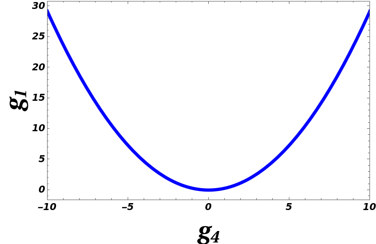
Figure 2: Variation of two body interaction as a function of BMF term (for $g_{3}=2$). The figure clearly suggests a parabolic dependence between these two interactions. The scale and the parameter value is in an arbitrary unit.

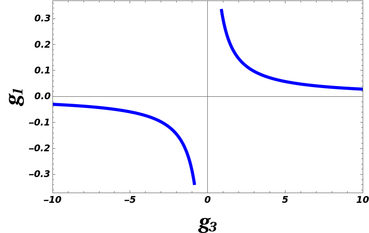
Figure 3: Variation of two-body interaction with three-body interaction strength for a fixed BMF interaction. The scale and the parameter value is in arbitrary units.

The final solution can be noted as,

$${\phi(z)=-\frac{g_{4}}{4g_{3}}+\Big{(}-\frac{V_{0}}{g_{3}}\Big{)}^{\frac{1}{4}}cn(z,m)}.$$ (24)

We have depicted the density distribution obtained from Eq.(24) for $m=0$ and $m=1$ in Fig. 4 and 5 respectively. The density variation is scaled by the density at the centre of trap, i.e., $|\phi_{0}|^{2}=|\phi(z=0)|^{2}=\left(\frac{g_{4}}{4g_{3}}\left(\left(\frac{|V_{0}|}{g_{3}}\right)^{1/4}\frac{4g_{3}}{g_{4}}-1\right)\right)^{2}$. For $m=0$ we obtain a periodic but binary amplitude distribution. The localized solution corresponding to $m=1$ depicts a $w$-soliton like structure with finite background density Debnath and Khan (2020).

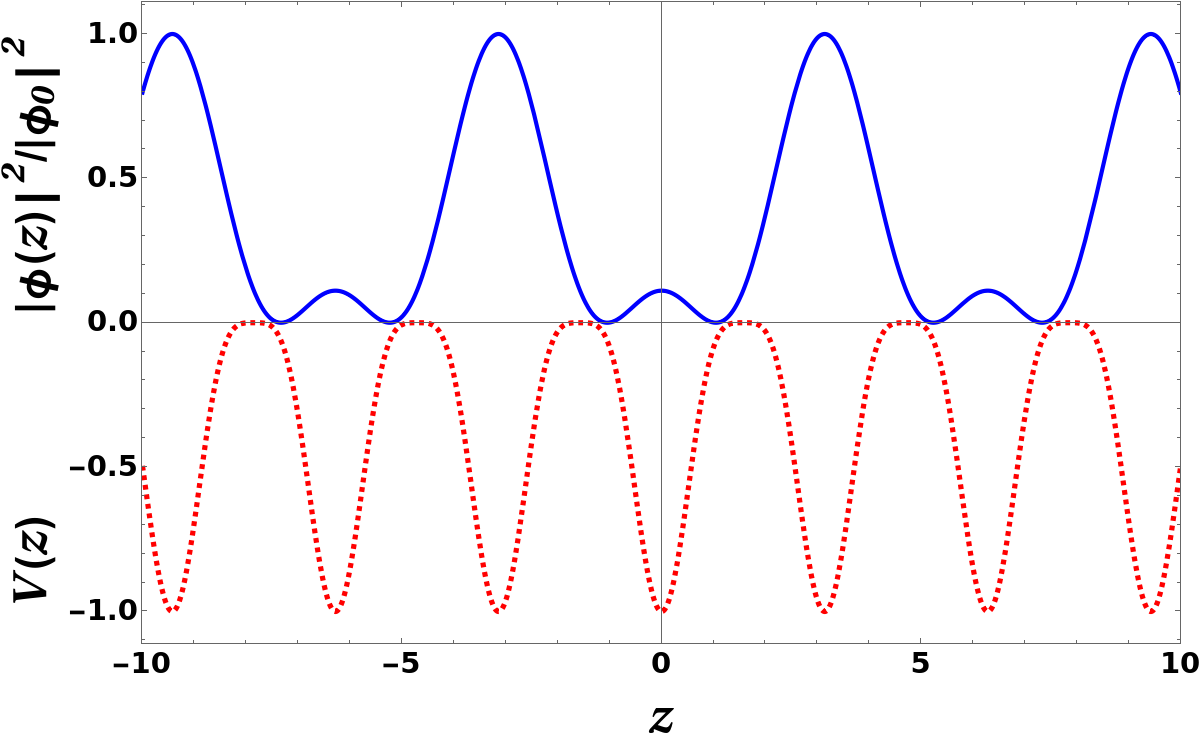
Figure 4: (Colour Online) The figure depicts the density distribution (blue solid line) and the variation of the external potential (red dotted line). The density is scaled by $|\phi_{0}|^{2}=|\phi(z=0)|^{2}$. For better visibility it is further scaled by the peak value. $V(z)$ is in the units of $V_{0}$. Here, $m=0$; $g_{4}=2$; $g_{3}=1$; $V_{0}=-1$. The parameter values are in arbitrary units.

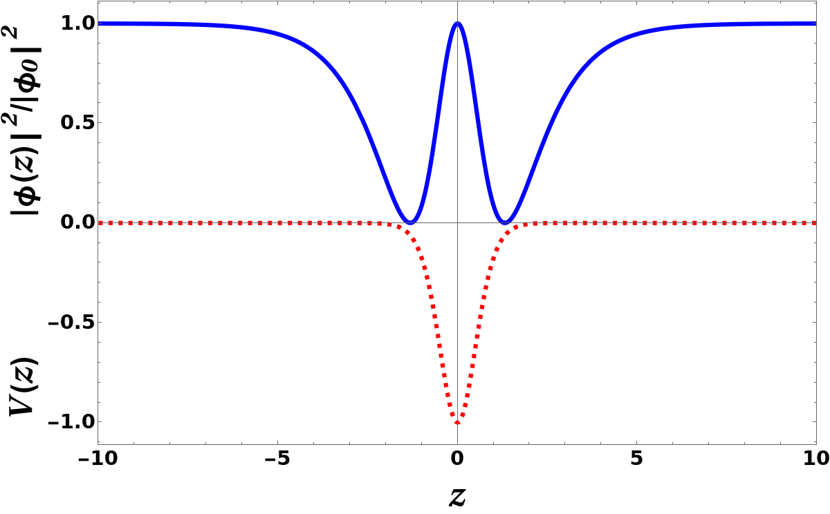
Figure 5: (Colour Online) Density distribution (blue solid line) and spatial variation of the external potential (red dotted line) is described here (scaled by $|\phi_{0}|^{2}$). The figure is prepared for $m=1$; $g_{4}=2$; $g_{3}=1$; $V_{0}=-1$. The parameter values are in arbitrary units.

Analytical Solution in 1D

We now repeat the similar strategy to solve QCQNLSE as described in Eq.(12). We assume, $\psi(x,t)=\phi(z)e^{-i\alpha t}$ with ansatz solution as $\phi(z)=Bcn(z,m)$. As described earlier, $z=\eta x$, and $\eta$ is the inverse of coherence length. We realize that to stabilize the system we require a super-lattice type potential such that, $V(z)=V_{0}cn(z,m)+V_{1}cn^{4}(z,m)$ Debnath et al. (2022).

Now Eq.(12) in $z$ variable can be written as,

$$\eta^{2}\frac{\partial^{2}\phi}{\partial z^{2}}+\phi(z)[\alpha-g_{1}|\phi(z)|^{2}-g_{2}|\phi(z)|-g_{3}|\phi(z)|^{4}$$

$$-V_{0}cn(z,m)-V_{1}cn^{4}(z,m)]=0$$ (25)

Inserting the ansatz solution we obtain a set of consistency equations which are noted as,

$$B\alpha-B\eta^{2}+2Bm\eta^{2} = 0$$ (26)

$$-B^{2}g_{2}-BV_{0} = 0$$ (27)

$$-B^{3}g_{1}-2Bm\eta^{2} = 0$$ (28)

$$-B^{5}g_{3}-BV_{1} = 0$$ (29)

An appropriate rearrangement will lead to the solution of the Eqs. (26), (27), (28) and (29). We yield a relationship between the equation parameters and solution parameters in the following form,

$${B=-\frac{V_{0}}{g_{2}}},\hskip 14.22636pt{g_{1}=-\frac{2m\eta^{2}}{V_{0}^{2}}g_{2}^{2}}.$$ (30)

Thus, the mean-field interaction is proportional to the square of the BMF interaction. Further, we obtain a constrained relationship between the interactions ($g_{2}$ and $g_{3}$) and potential strengths ($V_{0}$ and $V_{1}$) such that $\frac{g_{2}^{4}}{g_{3}}=-\frac{V_{0}^{4}}{V_{1}}$. The chemical potential and the inverse of coherence length reads:

$$\alpha = -\frac{V_{0}^{2}(1-2m)}{2m}\Big{(}\frac{g_{1}}{g_{2}^{2}}\Big{)},$$ (31)

$$\eta = \sqrt{\frac{\alpha}{1-2m}}.$$ (32)

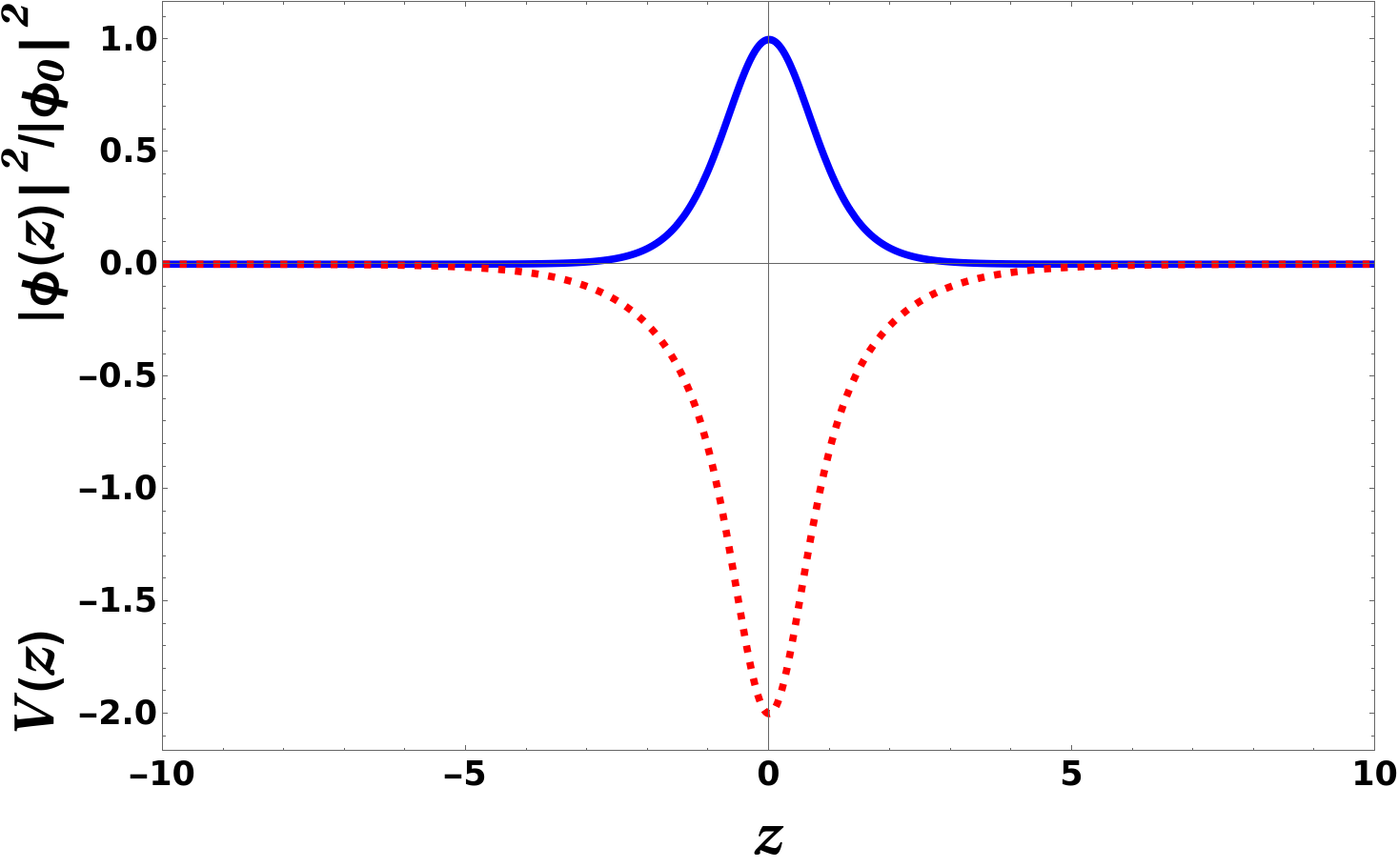
Figure 6: (Colour Online) Variation of density (blue solid line) and description of potential landscape (red dotted line) is illustrated here (with moduli parameter, $m=1$). The density is scaled by the centre of the trap density, i.e., $|\phi_{0}|^{2}=|\phi(z=0)|^{2}=(-V_{0}/g_{2})^{2}$. The potential is in units of $V_{0}$. All the parameters are in arbitrary units such that $g_{2}=1$; $V_{0}=-1$; $V_{1}=1$.

Therefore, the final solution turns out as,

$${\phi(z)=-\frac{V_{0}}{g_{2}}cn(z,m)}$$ (33)

A closer inspection of Eqs.(31) and (32) allows us to conclude that at $m=0$, $\eta\rightarrow\infty$ so to keep the dimensionless parameter $z$ finite, $x\rightarrow 0$. Also, Eq.(33) reveals to us that it is essential to have the BMF interaction for a physically acceptable solution. In Fig. 6 we depict the density distribution via blue solid line and external trap variation through red dotted line. The solution clearly manifests bright soliton like nature where $\phi(z)\rightarrow 0$ asymptotically. We also note the periodic solution against the backdrop of quasi periodic potential landscape in Fig. 7.

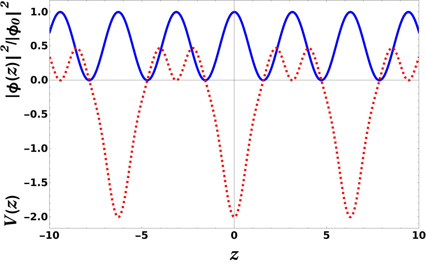
Figure 7: (Colour Online) The figure describes the periodic variation of the density mode (blue solid line) in a super-lattice like potential landscape (red dotted line). The moduli parameter or $m$ is considered as zero here. The density is scaled by the centre of the trap density, i.e., $|\phi_{0}|^{2}=|\phi(z=0)|^{2}=(-V_{0}/g_{2})^{2}$. The other parameters are in arbitrary units such as $g_{2}=1$; $V_{0}=-1$ and $V_{1}=1$.

Calculation of Surface Tension

Surface tension is a solely liquid property that allows it to resist an external force, due to the cohesive nature of its molecules. Hence, in the context of liquid formation in quantum gases, existence of surface tension can be regarded as one of the significant pieces of evidence as pointed out in Ref. Bulgac (2002).

In quantum gases, if the effective scattering length is attractive (say $a<0$) then energy per particle relation for a uniform condensate(i.e $E_{2}=\frac{1}{2}g_{2}\rho$ , where $g_{2}=\frac{4\pi\hbar^{2}a}{m}$), is unbounded and density be will unstable with respect to the density fluctuations. However, it was suggested that inclusion of three-body correlation effect changes the situation dramatically and predicted that stable droplet formation can be possible via surface tension calculation Bulgac (2002).

If two body scattering length is large enough(i.e $|a|>>r_{0}$, where, $r_{0}$ is the two body interaction radius) then there will be two independent dimensionless parameter $\rho a^{3}$ and $\rho r_{0}^{3}$. In this situation, three-body interaction starts playing significant role irrespective of the nature of two-body interaction (i.e., whether it is attractive or repulsive), eventually we observe emergence of three-body bound state which is commonly known as Efimov effect Efimov (1973). In this situation, the surface tension can be defined as,

$$\sigma=\int_{-\infty}^{\infty}dx[\epsilon(x)-\mu_{0}\rho(x)],$$ (34)

where $\epsilon(x)$ is the energy density and $\rho(x)$ is the density. Now applying Eq.(24) and Eq.(33) in Eq.(34) using the energy functional corresponding to Eq.(11) and Eq.(12) we can obtain the non zero surface tension for Q1D and 1D respectively,

$$\sigma_{Q1D} = \frac{1}{3}\sqrt{-\frac{V_{0}}{g_{3}}},$$ (35)

$$\sigma_{1D} = \frac{1}{3}\left(\frac{V_{0}}{g_{2}}\right)^{2}.$$ (36)

The calculation is carried out after carefully transforming the $x$ variable to $z$ variable.

Eq.(35) and Eq.(36) possess some common attributes while they are quite distinctive in nature as well. In both cases we find that the trapping potential has an important role to play and if $V_{0}=0$ then surface tension is zero which implies that the atoms can not form clusters to emerge as liquid-like state. However, one striking difference is, in Q1D three-body interaction is essential for non-zero surface tension while in 1D the BMF interaction plays that role. Fig. 8 describes that the surface tension is proportional to the inverse square root of three body interaction while in Fig. 9 we observe that the surface tension varies with the inverse square of BMF interaction. This implies that, in Q1D we should be able to yield quantum droplets even if we do not take into account BMF interaction which was precisely pointed out in Ref. Bulgac (2020), nevertheless in 1D system, we see a role reversal.

If we now look into the chronological perspective, the recent discussions on droplets are mainly from the perspective of BMF interaction; the earlier discussion was more in the context of interplay between two-body and three-body interactions. However, our current discussion suggests that BMF interaction is irreplaceable in 1D, while in Q1D, three-body interaction can induce liquid formation. Hence, based on the recent discussions on platicons (FTS) and dropletons Lobanov et al. (2021); Alotaibi et al. (2023), and our current observation, motivates us to characterize the Q1D liquid as platicon and 1D liquid as dropleton.

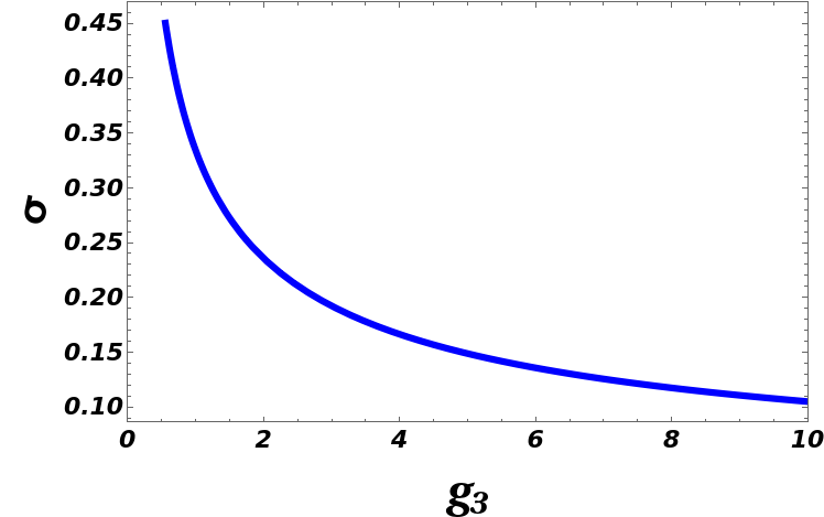
Figure 8: Variation of surface tension as a function of three body interaction in Q1D system. Here, $V_{0}$ is considered as $-1$ in arbitrary units.

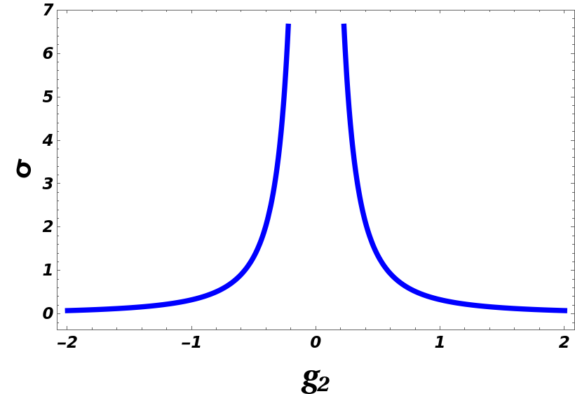
Figure 9: Variation of surface tension with BMF interaction in 1D system. Here, $V_{0}$ is considered as $-1$ in arbitrary units.

IV Conclusion

In recent years, we have observed significant interest in understanding liquid-like state formation in ultra-cold atomic gases due to the theoretical developments Petrov (2015); Petrov and Astrakharchik (2016); Ilg et al. (2018) and experimental verification Cabrera et al. (2018); Ferrier-Barbut et al. (2016); Wächtler and Santos (2016). The fundamental theoretical proposition suggests that the BMF interaction competes with the effective MF interaction to support the clustering of atoms. However, two decades ago a similar exotic phase was predicted theoretically by considering the competition of two-body and three-body interactions Bulgac (2002); Bedaque et al. (2003). In this article, we have tried to review both the perspectives in Q1D and 1D geometry through a pathelogical model.

We have already noted interesting differences in Q1D and 1D geometry from mathematical and physical perspective Debnath et al. (2022) when we include BMF interaction. We have noted that in Q1D, the dynamical equation boils down to a CQNLSE while in 1D it is QCNLSE. We have now included the three-body interaction in our calculation and obtained the cnoidal solutions. We know that the cnoidal functions can boil down to periodic or localized function based on their moduli parameter. Hence, to exploit this mathematical manoeuvrability we restrict our solutions to cnoidal functions only. Later, we calculate the corresponding surface tension associated with each dimension. Interestingly, we note that an external potential is invariably required for non-zero surface tension in both the cases. However, in Q1D, surface tension is independent of BMF interaction and we can have non-zero surface tension due to the competition between two-body and three-body interactions while in 1D, it is essential to have BMF interaction whereas three-body interaction appears redundant.

We hope our current analysis will shed some light in the context of dropleton and platicon and will also motivate some experiments to study these exotic phases in lower dimensions.

References

- Kadau et al. (2016) H. Kadau, M. Schmitt, M. Wenzel, C. Wink, T. Maier, I. Ferrier-Barbut, and T. Pfau, Nature 530, 194 (2016).
- Li et al. (2017) J.-R. Li, J. Lee, W. Huang, S. Burchesky, B. Shteynas, F. Ç. Top, A. O. Jamison, and W. Ketterle, Nature 543, 91 (2017).
- Cabrera et al. (2018) C. Cabrera, L. Tanzi, J. Sanz, B. Naylor, P. Thomas, P. Cheiney, and L. Tarruell, Science 359, 301 (2018).
- Chomaz et al. (2019) L. Chomaz, D. Petter, P. Ilzhöfer, G. Natale, A. Trautmann, C. Politi, G. Durastante, R. Van Bijnen, A. Patscheider, M. Sohmen, et al., Physical Review X 9, 021012 (2019).
- Böttcher et al. (2019) F. Böttcher, J.-N. Schmidt, M. Wenzel, J. Hertkorn, M. Guo, T. Langen, and T. Pfau, Physical Review X 9, 011051 (2019).
- Tanzi et al. (2019) L. Tanzi, E. Lucioni, F. Famà, J. Catani, A. Fioretti, C. Gabbanini, R. N. Bisset, L. Santos, and G. Modugno, Physical review letters 122, 130405 (2019).
- Donner (2019) T. Donner, Physics 12, 38 (2019).
- Petrov (2015) D. S. Petrov, Phys. Rev. Lett. 115, 155302 (2015).
- Petrov and Astrakharchik (2016) D. S. Petrov and G. E. Astrakharchik, Phys. Rev. Lett. 117, 100401 (2016).
- Lee et al. (1957) T. D. Lee, K. Huang, and C. N. Yang, Phys. Rev. 106, 1135 (1957).
- Ferrier-Barbut (2019) I. Ferrier-Barbut, Physics Today 72, 46 (2019).
- Bulgac (2002) A. Bulgac, Physical review letters 89, 050402 (2002).
- Bedaque et al. (2003) P. F. Bedaque, A. Bulgac, and G. Rupak, Physical Review A 68, 033606 (2003).
- Bulgac (2020) A. Bulgac, Physics Today 73, 10 (2020).
- Lobanov et al. (2021) V. E. Lobanov, A. E. Shitikov, R. R. Galiev, K. N. Min’kov, O. V. Borovkova, and N. M. Kondratiev, Physical Review A 104, 063511 (2021).
- Alotaibi et al. (2023) M. Alotaibi, L. Al Sakkaf, and U. Al Khawaja, Physics Letters A 487, 129120 (2023).
- Astrakharchik and Malomed (2018) G. E. Astrakharchik and B. A. Malomed, Phys. Rev. A 98, 013631 (2018).
- Debnath and Khan (2021) A. Debnath and A. Khan, Annalen der Physik 533, 2000549 (2021).
- Pu and Bigelow (1998) H. Pu and N. Bigelow, Physical review letters 80, 1130 (1998).
- Myatt et al. (1997) C. Myatt, E. Burt, R. Ghrist, E. A. Cornell, and C. Wieman, Physical Review Letters 78, 586 (1997).
- Ancilotto et al. (2018) F. Ancilotto, M. Barranco, M. Guilleumas, and M. Pi, Physical Review A 98, 053623 (2018).
- Cappellaro et al. (2018) A. Cappellaro, T. Macrì, and L. Salasnich, Physical Review A 97, 053623 (2018).
- Cheiney et al. (2018) P. Cheiney, C. R. Cabrera, J. Sanz, B. Naylor, L. Tanzi, and L. Tarruell, Phys. Rev. Lett. 120, 135301 (2018).
- Khaykovich et al. (2002) L. Khaykovich, F. Schreck, G. Ferrari, T. Bourdel, J. Cubizolles, L. D. Carr, Y. Castin, and C. Salomon, Science 296, 1290 (2002).
- Khan and Panigrahi (2013) A. Khan and P. K. Panigrahi, Journal of Physics B: Atomic, Molecular and Optical Physics 46, 115302 (2013).
- Debnath et al. (2022) A. Debnath, J. Tarun, and A. Khan, Journal of Physics B: Atomic, Molecular and Optical Physics 55, 025301 (2022).
- Efimov (1973) V. Efimov, Nuclear Physics A 210, 157 (1973).
- Abramowitz et al. (1988) M. Abramowitz, I. A. Stegun, and R. H. Romer, “Handbook of mathematical functions with formulas, graphs, and mathematical tables,” (1988).
- Debnath and Khan (2020) A. Debnath and A. Khan, The European Physical Journal D 74, 1 (2020).
- Ilg et al. (2018) T. Ilg, J. Kumlin, L. Santos, D. S. Petrov, and H. P. Büchler, Physical Review A 98, 051604 (2018).
- Ferrier-Barbut et al. (2016) I. Ferrier-Barbut, H. Kadau, M. Schmitt, M. Wenzel, and T. Pfau, Phys. Rev. Lett. 116, 215301 (2016).
- Wächtler and Santos (2016) F. Wächtler and L. Santos, Phys. Rev. A 93, 061603 (2016).