Regularized Exponentially Tilted Empirical Likelihood for Bayesian Inference

Abstract

Bayesian inference with empirical likelihood faces a challenge as the posterior domain is a proper subset of the original parameter space due to the convex hull constraint. We propose a regularized exponentially tilted empirical likelihood to address this issue. Our method removes the convex hull constraint using a novel regularization technique, incorporating a continuous exponential family distribution to satisfy a Kullback–Leibler divergence criterion. The regularization arises as a limiting procedure where pseudo-data are added to the formulation of exponentially tilted empirical likelihood in a structured fashion. We show that this regularized exponentially tilted empirical likelihood retains certain desirable asymptotic properties of (exponentially tilted) empirical likelihood and has improved finite sample performance. Simulation and data analysis demonstrate that the proposed method provides a suitable pseudo-likelihood for Bayesian inference. The implementation of our method is available as the R package retel. Supplementary materials for this article are available online.

Keywords: Bernstein–von Mises theorem; Convex hull; Entropy balancing; Kullback–Leibler divergence; Pseudo-data

1 Introduction

Statistical models defined through estimating equations and moment conditions allow semiparametric inferences on quantities of interest without distributional assumptions. Empirical likelihood (EL) (Owen, 1988; Qin & Lawless, 1994), a popular approach in the frequentist setting, enables nonparametric but still likelihood style inference. It shares many desirable properties with parametric likelihood, exhibiting Wilks’ phenomenon under mild conditions and allowing for Bartlett correction (DiCiccio et al., 1991). Moreover, confidence regions from EL have data-driven shapes and orientations.

EL is a member of the class of generalized empirical likelihoods (GEL) (Smith, 1997; Newey & Smith, 2004), which includes the exponential tilting of Efron (1981). Newey & Smith (2004) showed a duality between GEL and the class of minimum discrepancy methods (Cressie & Read, 1984; Corcoran, 1998). In this context, EL is formulated by finding a distribution supported on the sample that minimizes the Kullback–Leibler (KL) divergence to the empirical distribution, subject to moment constraints. Exponentially tilted empirical likelihood (ETEL) (Efron, 1981; Jing & Wood, 1996; Schennach, 2005) is obtained by combining exponential tilting and EL, which minimizes the reverse KL divergence.

Bayesian analysis of EL poses a challenge, as posterior inference via Bayes’ Theorem requires a complete specification of the sampling distribution or the likelihood function. Lazar (2003) proposed using EL as a replacement for the likelihood function in Bayesian inference. Through simulation, she showed that the EL-posterior distributions can exhibit strong similarities to traditional posterior distributions. Schennach (2005) strengthened the case for these methods by showing that ETEL arises as the limit of nonparametric Bayesian procedures with a particular type of prior favoring entropy-maximizing distributions. Chib et al. (2018) established a Bernstein–von Mises theorem for the Bayesian ETEL-posterior distribution, ensuring that the frequentist coverage of credible sets is asymptotically correct. Similar asymptotic results for EL were established by Sueishi (2022).

However, both EL and ETEL have an inherent limitation in that they are only defined on a proper subset of the original parameter space due to the convex hull constraint or empty set problem (Grendár & Judge, 2009). By convention, the likelihoods are set to zero for parameter values that violate the convex hull constraint. For Bayesian inference, the zeroes in the likelihood imply a restricted posterior domain. This is conceptually unsatisfactory as, with a larger sample size, the convex hull may expand and the likelihood become positive. Additionally, as the restricted domain is often non-convex (Chaudhuri et al., 2017), a more sophisticated posterior sampling scheme may be needed to fit the model.

To address these issues, various adjustments to EL have been suggested (Bartolucci, 2007; Chen et al., 2008; Tsao & Wu, 2013). Most relevant to our work, Chen et al. (2008) proposed the adjusted empirical likelihood (AEL), which adds a pseudo-observation in a way that satisfies the convex hull constraint for any given parameter value. This approach has been further developed by Emerson & Owen (2009) and Liu & Chen (2010), and it has been adapted for ETEL by Zhu et al. (2009) as the adjusted exponentially tilted empirical likelihood (AETEL).

In this paper, we propose a method to address the convex hull constraint for Bayesian ETEL. While previous proposals have primarily focused on EL and frequentist inference, our proposal builds upon the AEL framework, introducing notable distinctions. First, we extend the method to accommodate multiple pseudo observations with fractional weights, combining the approaches of weighted empirical likelihood (Glenn & Zhao, 2007) and an entropy balancing scheme (Hainmueller, 2012). Second, we pass to the limit, ensuring that the convex hull constraint is satisfied for all parameter values simultaneously. This resulting formulation naturally induces a form of regularization that removes the constraint. Our method’s main contributions encompass: (i) addressing the convex hull constraint for ETEL while retaining desirable asymptotic properties; (ii) enhancing stability and robustness of small-sample performance compared to existing methods; (iii) providing flexibility in Bayesian modelling and allowing one to incorporate a novel form of prior information.

This paper is organized as follows. In Section 2, we introduce the notation used in the paper and provide a brief overview of ETEL. Then, we propose a weighted version of ETEL that incorporates fractional pseudo-data with the maximum entropy reweighting scheme. In Section 3, we propose inducing regularization on the formulation of ETEL, exploring two equivalent approaches: (i) a limiting procedure with fractional pseudo-data and (ii) direct incorporation of a continuous exponential family distribution in the minimization of the KL divergence. We derive asymptotic properties of the proposed method. In Section 4, we evaluate the performance of the methods through simulation studies. In Section 5, we present an application to the estimation of median income for four-person families. Finally, we conclude with a discussion of directions for future research in Section 6. The proofs of the theoretical results are provided in the supplementary materials. The proposed method is implementation in the R package retel (Kim, 2024), available from the Comprehensive R Archive Network (CRAN) at https://cran.r-project.org/package=retel.

2 Weighted Exponentially Tilted Empirical Likelihood with Fractional Pseudo-Data

We begin by introducing ETEL, along with the setup and some notation. Let ${\mathcal{D}_{n}}={\{\bm{X}_{i}\}_{i=1}^{n}}$ denote independent ${d_{x}}$-dimensional observations from a complete probability space ${(\mathcal{X},\mathcal{F},P)}$ satisfying the moment condition: ${\textnormal{E}_{P}[\bm{g}(\bm{X}_{i},\bm{\theta})]=\bm{0}}$, where ${\bm{g}}:{\mathbb{R}^{d_{x}}\times\Theta}\mapsto{\mathbb{R}^{p}}$ is an estimating function with the true parameter value ${\bm{\theta}_{0}}\in{\Theta}\subset\mathbb{R}^{p}$. Consider a discrete probability distribution ${P_{0}}$ that is absolutely continuous with respect to the empirical distribution ${P_{n}}$. The KL divergence from ${P_{n}}$ to ${P_{0}}$ is ${D_{KL}(P_{0}\ \|\ P_{n})=\sum_{i=1}^{n}p_{i}\log(np_{i})}$, where ${p_{i}}$ are probabilities attached to the observations by ${P_{0}}$. By minimizing the KL divergence subject to the constraints in the moment condition, we obtain a unique set of ${p_{i}}$ and the associated distribution. For a given ${\bm{\theta}}$, the maximization problem

$$\max_{p_{1},\dots,p_{n}}\left\{\sum_{i=1}^{n}\left(-p_{i}\log\left(np_{i}\right)\right)\mathrel{}\middle|\mathrel{}\sum_{i=1}^{n}p_{i}\bm{g}\left(\bm{X}_{i},\bm{\theta}\right)=\bm{0},\quad p_{i}\geq 0,\quad\sum_{i=1}^{n}p_{i}=1\right\}$$

yields a unique solution ${(p_{1}(\bm{\theta}),\dots,p_{n}(\bm{\theta}))}$, and ETEL is defined as ${L_{ET}(\bm{\theta})=\prod_{i=1}^{n}p_{i}(\bm{\theta})}$. By applying the method of Lagrange multipliers, we obtain

$$p_{i}\left(\bm{\theta}\right)=\frac{\exp\left({\bm{\lambda}_{ET}}^{\top}\bm{g}\left(\bm{X}_{i},\bm{\theta}\right)\right)}{\sum_{j=1}^{n}\exp\left({\bm{\lambda}_{ET}}^{\top}\bm{g}\left(\bm{X}_{j},\bm{\theta}\right)\right)},$$

where ${\bm{\lambda}_{ET}}\equiv{\bm{\lambda}_{ET}(\bm{\theta})}$ solves the equation ${n^{-1}\sum_{i=1}^{n}\exp({\bm{\lambda}}^{\top}\bm{g}(\bm{X}_{i},\bm{\theta}))\bm{g}(\bm{X}_{i},\bm{\theta})=\bm{0}}$. The dual problem provides the solution: ${\bm{\lambda}_{ET}=\operatorname*{\arg\!\min}_{\bm{\lambda}\in\mathbb{R}^{p}}\sum_{i=1}^{n}\exp(\bm{\lambda}^{\top}\bm{g}(\bm{X}_{i},\bm{\theta}))}$. By construction, an ${M}$-estimator ${\widehat{\bm{\theta}}}$ that solves ${n^{-1}\sum_{i=1}^{n}\bm{g}(\bm{X}_{i},\bm{\theta})}={\bm{0}}$ maximizes ETEL (Yiu et al., 2020).

In the Bayesian framework, ETEL can be used with a prior ${\pi(\bm{\theta})}$ to define the ETEL-posterior distribution $\pi(\bm{\theta}\mid\mathcal{D}_{n})\propto\pi(\bm{\theta})L_{ET}(\bm{\theta})$. Schennach (2005) showed that when all observations are distinct, ${L_{ET}(\bm{\theta})}$ can be obtained as the limit of a nonparametric Bayesian procedure. Her procedure involves assigning a mixture of uniform densities as a nonparametric prior on ${P}$ that satisfies the moment condition and then marginalizing over the nuisance parameters. The convex hull constraint serves as the implicit constraint in the primal optimization problem, indicating that the interior of the convex hull of ${\{\bm{g}(\bm{X}_{i},\bm{\theta})\}_{i=1}^{n}}$, denoted by ${\textnormal{Conv}_{n}(\bm{\theta})}$, must contain ${\bm{0}}$. Consequently, the (posterior) domain of ETEL is restricted to ${\Theta_{n}}={\{\bm{\theta}\in\Theta:\bm{0}\in\textnormal{Conv}_{n}(\bm{\theta})\}}$ so that even a ${100\%}$ credible set may fail to contain ${\bm{\theta}_{0}}$. In general, ${\Theta_{n}}$ is nonconvex and is challenging to identify. Simulation methods to fit the models, such as Markov chain Monte Carlo or Hamiltonian Monte Carlo, require long runs and may or may not be effective (Chaudhuri et al., 2017; Yu & Bondell, 2023), leading to potential undercoverage issues and unreliable inference.

To address the convex hull constraint for EL, the AEL approach introduces a pseudo-observation that depends on ${\bm{\theta}}$. Here and throughout, we use ${\bm{g}_{i}(\bm{\theta})}={\bm{g}(\bm{X}_{i},\bm{\theta})}$, ${i}={1,\dots,n}$, for notational convenience. The pseudo-observation has

$$\bm{g}_{n+1}(\bm{\theta})=-\frac{a_{n}}{n}\sum_{i=1}^{n}\bm{g}_{i}(\bm{\theta}),$$ (1)

where ${a_{n}}>{0}$. Properties of the sequence ${a_{n}}$ are used to establish asymptotic results. The addition of ${\bm{g}_{n+1}(\bm{\theta})}$ ensures that the convex hull constraint is satisfied for each ${\bm{\theta}}\in{\Theta}$.

Emerson & Owen (2009) and Liu & Chen (2010) proposed adding two pseudo-observations to improve the coverage accuracy of confidence regions obtained from AEL. Yu & Bondell (2023) established a Bernstein–von Mises theorem for Bayesian AEL. While the AEL approach is directly applicable to ETEL for fixing the convex hull constraint for a particular ${\bm{\theta}}$, it may introduce irregularities throughout ${\Theta}$ in the resulting posterior distribution when applied to Bayesian analysis, since it involves a preliminary entropy maximization step in constructing the likelihood function. Incorporating one or two pseudo-observations, specific to each ${\bm{\theta}}$, and treating them on par with actual observations may contribute to these irregularities.

As an initial step towards addressing the convex hull constraint for ETEL and establishing a connection with the regularization method discussed in Section 3, we propose a weighted exponentially tilted empirical likelihood (WETEL) approach with fractional pseudo-data. Our approach extends the AEL method by incorporating multiple pseudo-observations, in combination with the entropy balancing scheme of Hainmueller (2012). Entropy balancing is a data preprocessing technique used to achieve covariate balance in observational studies with a binary treatment and in survey sampling. The preprocessing step involves applying a maximum-entropy reweighting scheme to ensure that the reweighted data satisfy a set of moment conditions. In the context of our framework, the pseudo-data can be seen as providing additional information for the analysis.

We introduce a fixed number, ${m}\in\mathbb{N}$, of pseudo-data denoted as ${\bm{g}_{n+j}(\bm{\theta})}\in{\mathbb{R}^{p}}$ for ${j}={1,\dots,m}$. The use of the estimating function ${\bm{g}}$ for the pseudo-data is for notational consistency. Apart from their dependence on ${\bm{\theta}}$, they need not necessarily be related to the observed data or estimating function. At this stage, we do not discuss any specific strategy for creating the pseudo-data. Instead, for our current purposes, we simply assume that the augmented data, comprising both the observed data and pseudo-data, satisfy the convex hull constraint.

Let ${w_{i}}$ be the base weight for the ${i}$th observation in the augmented data, such that ${\sum_{i=1}^{N}w_{i}}={1}$, with ${N}={n+m}$. We consider the following maximum-entropy reweighting scheme:

$$\max_{p_{1},\dots,p_{N}}\left\{\sum_{i=1}^{N}\left(-p_{i}\log\left(\frac{p_{i}}{w_{i}}\right)\right)\mathrel{}\middle|\mathrel{}\sum_{i=1}^{N}p_{i}\bm{g}_{i}\left(\bm{\theta}\right)=\bm{0},\quad p_{i}\geq 0,\quad\sum_{i=1}^{N}p_{i}=1\right\}.$$

This scheme is equivalent to minimizing ${D_{KL}(P_{0}\ \|\ P_{w})}$ subject to the constraints above, where ${P_{w}}$ is the weighted empirical distribution. Both ${P_{0}}$ and ${P_{w}}$ are now supported on the augmented data. The objective function is modified to account for the weights and pseudo-data, and the moment condition is matched by the augmented data. The method of Lagrange multipliers yields

$$p_{i}\left(\bm{\theta}\right)=\frac{w_{i}\exp\left({\bm{\lambda}_{WET}}^{\top}\bm{g}_{i}\left(\bm{\theta}\right)\right)}{\sum_{j=1}^{N}w_{j}\exp\left({\bm{\lambda}_{WET}}^{\top}\bm{g}_{j}\left(\bm{\theta}\right)\right)},$$

where ${\bm{\lambda}_{WET}}={\operatorname*{\arg\!\min}_{\bm{\lambda}\in\mathbb{R}^{p}}\sum_{i=1}^{N}w_{i}\exp({\bm{\lambda}}^{\top}\bm{g}_{i}(\bm{\theta}))}$.

Next, building upon the weighted EL approach proposed by Glenn & Zhao (2007), we formulate the likelihood function as ${L_{WET}(\bm{\theta})}={\prod_{i=1}^{N}{p_{i}(\bm{\theta})}^{Nw_{i}}}$. Based on the inequality ${\prod_{i=1}^{N}{p_{i}(\bm{\theta})}^{Nw_{i}}}\leq{\prod_{i=1}^{N}w_{i}^{Nw_{i}}}$ for any solution ${p_{i}(\bm{\theta})}$, the likelihood ratio function of WETEL can be defined as ${R_{WET}\left(\bm{\theta}\right)}={\prod_{i=1}^{N}(p_{i}(\bm{\theta})/{w_{i}})^{Nw_{i}}}$. Consequently, the maximum WETEL estimator ${\widehat{\bm{\theta}}_{w}}$ is obtained by solving the equation ${\sum_{i=1}^{N}w_{i}\bm{g}_{i}(\bm{\theta})}={\bm{0}}$. When using uniform weights with $w_{i}={1/N}$, the resulting WETEL reduces to ETEL with the pseudo-data included. However, in finite sample settings, the size of ${m}$ relative to ${n}$, the pseudo-data specification, and the choice of weights can lead to substantial differences between WETEL and ETEL. To prevent this, we treat all pseudo-data as a single observation and assign fractional weights to them. Specifically, we set the weights as follows:

$$w_{i}=\begin{dcases*}\frac{1}{n+1}&$\left(i=1,\dots,n\right)$,\\[4.30554pt] \frac{1}{m\left(n+1\right)}&$\left(i=n+1,\dots,n+m\right)$.\end{dcases*}$$ (2)

This weight specification balances the contribution from the pseudo-data with the modified multiplier: ${\bm{\lambda}_{WET}}={\operatorname*{\arg\!\min}_{\bm{\lambda}\in\mathbb{R}^{p}}\{\sum_{i=1}^{n}\exp({\bm{\lambda}}^{\top}\bm{g}_{i}(\bm{\theta}))+m^{-1}\sum_{i=n+1}^{n+m}\exp({\bm{\lambda}}^{\top}\bm{g}_{i}(\bm{\theta}))\}}$.

Since WETEL is a generalization of ETEL with finite pseudo-data, it preserves the major asymptotic properties of ETEL as ${n}\to{\infty}$. Let ${\bm{G}}={\textnormal{E}_{P}[\partial_{\bm{\theta}}\bm{g}_{i}(\bm{\theta}_{0})]}$, ${\bm{V}}={\textnormal{E}_{P}[\bm{g}_{i}(\bm{\theta}_{0}){\bm{g}_{i}(\bm{\theta}_{0})}^{\top}]}$, and ${\bm{\Omega}}={({\bm{G}}^{\top}{\bm{V}}^{-1}\bm{G})^{-1}}$, where ${\partial_{\bm{\theta}}\bm{g}_{i}(\bm{\theta}_{0})}$ denotes the Jacobian matrix of ${\bm{g}_{i}(\bm{\theta})}$ evaluated at ${\bm{\theta}_{0}}$. Moreover, the Euclidean norm for vectors is denoted by ${|\cdot|}$, and the Frobenius norm for matrices is denoted by ${\|\cdot\|}$. We also use ${N(\bm{\mu},\bm{\Sigma})}$ to represent a multivariate normal distribution with mean ${\bm{\mu}}$ and covariance matrix ${\bm{\Sigma}}$, and ${\chi^{2}_{p}}$ to represent a chi-square distribution with ${p}$ degrees of freedom. We present the following technical conditions required to establish theoretical results.

Condition 1.

The parameter space ${\Theta}$ is compact, with ${\bm{\theta}_{0}}$ an interior point of ${\Theta}$ and the unique solution to ${\textnormal{E}_{P}[\bm{g}_{i}(\bm{\theta})]}={\bm{0}}$.

Condition 2.

With probability ${1}$, ${\bm{g}_{i}(\bm{\theta})}$ is continuous at each ${\bm{\theta}}\in{\Theta}$, continuously differentiable in a neighborhood ${\mathcal{N}}$ of ${\bm{\theta}_{0}}$, and ${\textnormal{E}_{P}[\sup_{\bm{\theta}\in\mathcal{N}}\|\partial_{\bm{\theta}}\bm{g}_{i}(\bm{\theta})\|]}<{\infty}$.

Condition 3.

${\textnormal{rank}({\bm{G}})}={\textnormal{rank}({\bm{V}})}={p}$.

Condition 4.

For some ${\alpha}>{3}$, ${\textnormal{E}_{P}[\sup_{\bm{\theta}\in\Theta}|\bm{g}_{i}(\bm{\theta})|^{\alpha}]}<{\infty}$.

These conditions are standard regularity conditions used to study the asymptotic behavior of GEL; see, for example, Newey & Smith (2004). We establish that the discrepancies between ETEL and WETEL, in terms of estimators and Lagrange multipliers, become asymptotically negligible.

Proposition 1.

Under Conditions 1, 2, 3 and 4, ${\widehat{\bm{\theta}}_{w}-\widehat{\bm{\theta}}}={o_{P}(n^{-1/2})}$ and ${\bm{\lambda}_{WET}(\bm{\theta}_{0})}-{\bm{\lambda}_{ET}(\bm{\theta}_{0})}={O_{P}(n^{-1})}$.

Consequently, WETEL shares with GEL first-order asymptotic properties.

Theorem 1.

Under Conditions 1, 2, 3 and 4, ${n^{1/2}(\widehat{\bm{\theta}}_{w}-\bm{\theta}_{0})}$ converges in distribution to ${N(\bm{0},\bm{\Omega})}$ as ${n}\to{\infty}$, and ${-2\log R_{WET}(\bm{\theta}_{0})}$ converges in distribution to ${\chi^{2}_{p}}$ as ${n}\to{\infty}$.

3 Regularized Exponentially Tilted Empirical Likelihood

In Section 2, we did not explicitly discuss the specification of pseudo-data for WETEL. When ${m}$ is fixed, the convex hull constraint issue may arise in WETEL, where ${\bm{0}}\notin{\textnormal{Conv}_{N}(\bm{\theta})}$ for certain values of ${\bm{\theta}}$, unless the pseudo-data are carefully specified. Even if we adopt a strategy like the one in Equation 1, the limitation remains because the specification of pseudo-data, regardless of careful selection or the magnitude of ${m}$, still needs to depend on the observed data and parameter values. In this sense, the pseudo-data approach can be viewed as an ad-hoc solution that pragmatically addresses the issue but does not fully resolve the underlying challenge associated with a finite ${m}$.

In this section, we consider a procedure where ${m}$ tends to infinity, enabling the pseudo-data to represent a continuous distribution in the limit. Since ETEL induces an exponential family of distributions supported on the data, a natural choice for the pseudo-data is a continuous exponential family distribution. To accomplish this, we introduce an auxiliary random variable ${\widetilde{\bm{g}}}\sim{N(\bm{\mu},\bm{\Sigma})}$ with known ${\bm{\mu}}$ and ${\bm{\Sigma}}$, where ${\bm{\Sigma}}$ is assumed to be of full rank. The pseudo-data ${\{\widetilde{\bm{g}}_{1},\widetilde{\bm{g}}_{2},\dots\}}$ may be selected as appropriate quantiles of ${N(\bm{\mu},\bm{\Sigma})}$, aiming to approximate the distribution as ${m}$ increases. For the purposes of our discussion, we assume that the pseudo-data are independent samples from ${N(\bm{\mu},\bm{\Sigma})}$, while treating the sample size ${n}$ and the parameter ${\bm{\theta}}$ as fixed.

Using the fractional weights in Equation 2, we introduce a sequence of stochastic minimization problems for WETEL: ${\min_{\bm{\lambda}\in\mathbb{R}^{p}}c_{m}(\bm{\lambda})}={\min_{\bm{\lambda}\in\mathbb{R}^{p}}\{d_{n}(\bm{\theta},\bm{\lambda})+p_{m}(\bm{\lambda})\}}$ for ${m}={1,2,\dots}$, where ${d_{n}(\bm{\theta},\bm{\lambda})}={\sum_{i=1}^{n}\exp(\bm{\lambda}^{\top}\bm{g}_{i}(\bm{\theta}))}$ and ${p_{m}(\bm{\lambda})}={m^{-1}\sum_{j=1}^{m}\exp(\bm{\lambda}^{\top}\widetilde{\bm{g}}_{j})}$. It follows from the independent sampling that ${p_{m}(\bm{\lambda})}\to{p(\bm{\lambda})}$ with probability ${1}$ as ${m}\to{\infty}$, where ${p(\bm{\lambda})}={\exp(\bm{\lambda}^{\top}\bm{\mu}+\bm{\lambda}^{\top}\bm{\Sigma}\bm{\lambda}/2)}$ is the moment-generating function of ${\widetilde{\bm{g}}}$. This suggests directly considering the following minimization problem:

$$\min_{\bm{\lambda}\in\mathbb{R}^{p}}c\left(\bm{\lambda}\right)=\min_{\bm{\lambda}\in\mathbb{R}^{p}}\left\{d_{n}\left(\bm{\theta},\bm{\lambda}\right)+p\left(\bm{\lambda}\right)\right\},$$ (3)

with the minimization performed after taking the limit. Then, the sequence of minimization problems can be viewed as a discretization of the population version of the minimization problem. Such a setting can be commonly found in applications of stochastic programming (Wets, 1974; Dupačová, 1992), equipped with epi-convergence (Dupačová & Wets, 1988; King & Wets, 1991; Rockafellar & Wets, 2009). We refer to this method as regularized exponentially tilted empirical likelihood (RETEL) and introduce the corresponding multiplier ${\bm{\lambda}_{RET}=\operatorname*{\arg\!\min}_{\bm{\lambda}\in\mathbb{R}^{p}}\{d_{n}(\bm{\theta},\bm{\lambda})+p(\bm{\lambda})\}}$.

From the convexity and lower semicontinuity of ${\exp(\bm{\lambda}^{\top}\widetilde{\bm{g}})}$, it is shown that ${p_{m}(\bm{\lambda})}$ epi-converges to ${p(\bm{\lambda})}$ as ${m}\to{\infty}$ with probability ${1}$ (see, for example, Artstein & Wets, 1995, Theorem 2.3). This establishes the consistency of the minimizers with the following intermediate result:

Proposition 2.

Under Condition 2, with probability ${1}$, the minimization problem in Equation 3 has a unique global minimizer ${\bm{\lambda}_{RET}}$ for each ${\bm{\theta}}\in{\Theta}$. Additionally, for any ${\epsilon_{m}}\downarrow{0}$, we have ${\lim_{m\to\infty}\left\{\epsilon_{m}\textnormal{-}\operatorname*{\arg\!\min}_{\bm{\lambda}\in\mathbb{R}^{p}}c_{m}\left(\bm{\lambda}\right)\right\}=\{\bm{\lambda}_{RET}\}}$, where ${\{\epsilon_{m}\textnormal{-}\operatorname*{\arg\!\min}_{\bm{\lambda}\in\mathbb{R}^{p}}c_{m}(\bm{\lambda})\}}={\{\bm{\lambda}\mid c_{m}(\bm{\lambda})\leq\inf_{\bm{\lambda}\in\mathbb{R}^{p}}c_{m}(\bm{\lambda})+\epsilon_{m}\}}$.

With probability ${1}$, ${\bm{\lambda}_{RET}}$ is a limit point of the sequence of approximate solutions to the minimization problems. For any finite ${m}$, ${\operatorname*{\arg\!\min}_{\bm{\lambda}\in\mathbb{R}^{p}}c_{m}(\bm{\lambda})}$ may not exist with positive probability. However, the existence and uniqueness of ${\bm{\lambda}_{RET}}$ are guaranteed by the strict convexity of ${p(\bm{\lambda})}$, which acts as a penalty that regularizes ${\bm{\lambda}}$ and prevents ${|\bm{\lambda}|}$ from diverging, regardless of whether ${\bm{0}}\in{\textnormal{Conv}_{n}(\bm{\theta})}$. Figure 1 shows an example where ${\lambda_{WET}}$ converges to ${\lambda_{RET}}$ as a sequence of pseudo-data approximates a normal distribution.

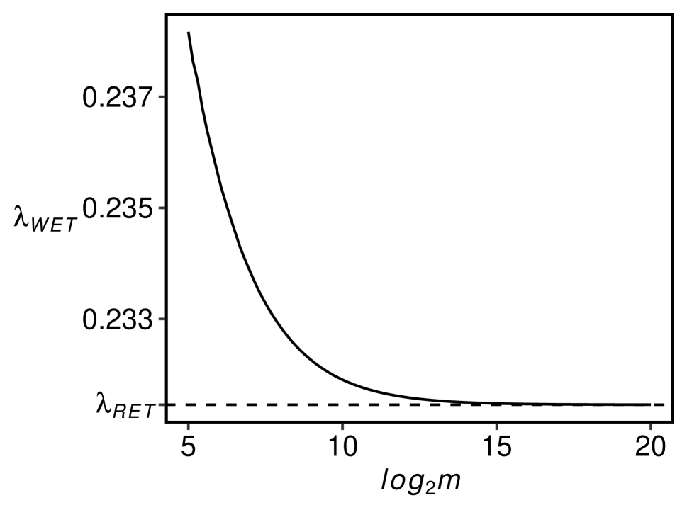
(a)

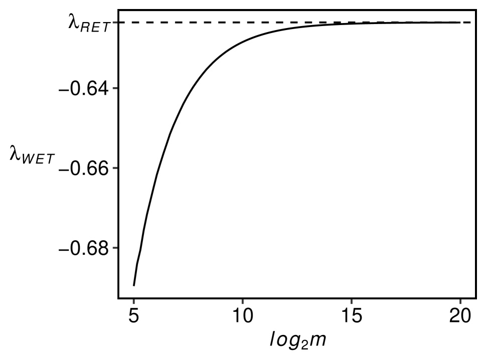
(b)

Figure 1: Plots of ${\lambda_{WET}(\theta)}$ versus ${\log_{2}{m}}$ for the mean parameter ${\theta}$. With two observations ${-2}$ and ${2}$ fixed, the convex hull constraint is satisfied at ${\theta}={1}$ in (a) and violated at ${\theta}={3}$ in (b). For each ${m}$, the pseudo-data are generated as the ${k/(m+1)}$ quantile of the standard normal distribution for ${k}={1,\dots,m}$. When the convex hull constraint is satisfied, ${\lambda_{WET}}$ converges faster to the respective ${\lambda_{RET}}$ (horizontal dashed lines).

The choice of ${\bm{\mu}}$ and ${\bm{\Sigma}}$ in ${p(\bm{\lambda})}$ depends on the requirements of a specific application, and each choice uniquely determines the shape and curvature of ${p(\bm{\lambda})}$. One simple option is to set ${\bm{\mu}}={\bm{0}}$ and ${\bm{\Sigma}}={\bm{I}_{p}}$, where ${\bm{I}_{p}}$ denotes the ${p\times p}$ identity matrix. More generally, we can consider

$$p_{n}\left(\bm{\theta},\bm{\lambda}\right)=\tau_{n}\exp\left(\bm{\lambda}^{\top}\bm{\mu}_{n,\bm{\theta}}+\frac{1}{2}\bm{\lambda}^{\top}\bm{\Sigma}_{n,\bm{\theta}}\bm{\lambda}\right),$$ (4)

and the corresponding minimization problem in Equation 3 becomes:

$$\min_{\bm{\lambda}\in\mathbb{R}^{p}}c_{n}\left(\bm{\theta},\bm{\lambda}\right)=\min_{\bm{\lambda}\in\mathbb{R}^{p}}\left\{d_{n}\left(\bm{\theta},\bm{\lambda}\right)+p_{n}\left(\bm{\theta},\bm{\lambda}\right)\right\},$$ (5)

with the solution still denoted by ${\bm{\lambda}_{RET}}$. Here, ${\tau_{n}}>{0}$ is a tuning parameter that controls the strength of ${p(\bm{\lambda})}$ as a penalty. The parameters ${\bm{\mu}_{n,\bm{\theta}}}$ and ${\bm{\Sigma}_{n,\bm{\theta}}}$, which may vary with ${n}$ and ${\bm{\theta}}$, can be drawn from prior information, allowing for more flexibility in the regularization.

Note that the description of the regularization suppresses an implicit connection to ${\bm{\theta}}$. For example, when considering the mean parameter ${\bm{\theta}}$, setting ${\bm{\mu}_{n,\bm{\theta}}}={\bm{0}}$ and ${\bm{\Sigma}_{n,\bm{\theta}}}={\bm{I}_{p}}$ corresponds to assuming a latent normal distribution $N(\bm{\theta},\bm{I}_{p})$ at each ${\bm{\theta}}$. On the other hand, changing to ${\bm{\mu}_{n,\bm{\theta}}}={\overline{\bm{X}}-\bm{\theta}}$ introduces $N(\overline{\bm{X}},\bm{I}_{p})$ centered at the sufficient statistic ${\overline{\bm{X}}}$, making the regularization invariant with respect to ${\bm{\theta}}$. In this case, the two choices will lead to considerably different ${\bm{\lambda}_{RET}}$ for ${\bm{\theta}}$ lying outside the convex hull of the observed data.

From an operational perspective, any function ${p(\cdot)}:{\mathbb{R}^{p}}\mapsto{\mathbb{R}_{>0}}$ that increases superlinearly with ${|\bm{\lambda}|}$ can be considered to ensure a finite ${\bm{\lambda}_{RET}}$. This penalty method can also be extended to other GEL methods that share the Cressie–Read family of discrepancies. However, we focus on ETEL due to its connection to the exponential family it generates (Yiu et al., 2020) and to the auxiliary continuous exponential family distribution that is naturally introduced.

In the following, we present an alternative approach to formulating the minimization problem in Equation 5. This approach does not involve the concept of a sequence of procedures with pseudo-data but instead directly considers a mixture of a normal and a multinomial distribution supported on the data. For a given ${\bm{\lambda}}$, we apply exponential tilting to the ${N(\bm{\mu}_{n,\bm{\theta}},\bm{\Sigma}_{n,\bm{\theta}})}$ distribution of ${\widetilde{\bm{g}}}$, resulting in the ${\bm{\lambda}}$-tilted distribution ${N(\bm{\mu}_{n,\bm{\theta}}+\bm{\Sigma}_{n,\bm{\theta}}\bm{\lambda},\bm{\Sigma}_{n,\bm{\theta}})}$. We denote the corresponding random variable as ${\widetilde{\bm{g}}_{\bm{\lambda}}}$. To formulate the problem, we consider two probability distributions:

$$\widetilde{P}_{n}=\frac{n}{n+\tau_{n}}P_{n}+\frac{\tau_{n}}{n+\tau_{n}}N\left(\bm{\mu}_{n,\bm{\theta}},\bm{\Sigma}_{n,\bm{\theta}}\right),\quad\widetilde{P}_{\bm{\lambda}}=\left(1-p_{c}\right)P_{0}+p_{c}N\left(\bm{\mu}_{n,\bm{\theta}}+\bm{\Sigma}_{n,\bm{\theta}}\bm{\lambda},\bm{\Sigma}_{n,\bm{\theta}}\right),$$

where each distribution is defined as a convex mixture of a discrete and a continuous distribution. The constant ${p_{c}}$ in ${\widetilde{P}_{\bm{\lambda}}}$ represents the probability assigned to the tilted distribution. The following result parallels the idea that ${D_{KL}({P}_{0}\ \|\ {P}_{n})}$ is minimized by ETEL.

Proposition 3.

For any ${\bm{\theta}}\in{\Theta}$, the minimization problem in Equation 5 is the dual problem of minimizing ${D_{KL}(\widetilde{P}_{\bm{\lambda}}\|\ \widetilde{P}_{n})}$ with respect to ${p_{i}}$, ${i}={1,\dots,n}$, and ${p_{c}}$, subject to $\sum_{i=1}^{n}p_{i}\bm{g}_{i}(\bm{\theta})+p_{c}\textnormal{E}_{\widetilde{P}_{\bm{\lambda}}}[{\widetilde{\bm{g}}_{\bm{\lambda}}}]={\bm{0}}$, ${p_{c}}\geq{0}$, ${p_{i}}\geq{0}$, and ${\sum_{i=1}^{n}p_{i}+p_{c}}={1}$.

As a consequence, the optimal values of ${p_{i}(\bm{\theta})}$ and ${p_{c}(\bm{\theta})}$ can be expressed as follows:

$$p_{i}\left(\bm{\theta}\right)=\frac{\exp\left({\bm{\lambda}_{RET}}^{\top}\bm{g}_{i}\left(\bm{\theta}\right)\right)}{c_{n}\left(\bm{\theta},\bm{\lambda}_{RET}\right)}\quad\left(i=1,\dots,n\right),\quad p_{c}\left(\bm{\theta}\right)=\frac{p_{n}\left(\bm{\theta},\bm{\lambda}_{RET}\right)}{c_{n}\left(\bm{\theta},\bm{\lambda}_{RET}\right)},$$

where ${\bm{\lambda}_{RET}}$ is the solution to the equation:

$$\sum_{i=1}^{n}\exp\left(\bm{\lambda}^{\top}\bm{g}_{i}\left(\bm{\theta}\right)\right)\bm{g}_{i}\left(\bm{\theta}\right)+p_{n}\left(\bm{\theta},\bm{\lambda}\right)\left(\bm{\mu}_{n,\bm{\theta}}+\bm{\Sigma}_{n,\bm{\theta}}\bm{\lambda}\right)=\bm{0}.$$ (6)

The formulations presented above suggest the possibility of using other exponential family distributions without modification. However, in this context, we proceed with normal distributions since the focus is to expand the domain to the entire parameter space for any estimating function. Furthermore, the normal distribution has the unique property of being the maximum entropy distribution among all distributions with a given mean and covariance (Cover & Thomas, 2006, Theorem 8.6.5).

Once we have determined ${\bm{\lambda}_{RET}}$, we define the likelihood and likelihood ratio functions as follows:

$$L_{RET}\left(\bm{\theta}\right)=p_{c}\left(\bm{\theta}\right)\prod_{i=1}^{n}p_{i}\left(\bm{\theta}\right),\quad R_{RET}\left(\bm{\theta}\right)=\left(\frac{n+\tau_{n}}{\tau_{n}}p_{c}\left(\bm{\theta}\right)\right)\prod_{i=1}^{n}\left(n+\tau_{n}\right)p_{i}\left(\bm{\theta}\right).$$ (7)

RETEL differs from penalty approaches for EL (Tang & Leng, 2010; Leng & Tang, 2012; Chang et al., 2018), where a penalty term is added to the empirical log-likelihood ratio to induce sparsity in the solution ${\widehat{\bm{\theta}}}$. Instead, RETEL aims to regularize the behavior of the multiplier ${\bm{\lambda}}$ before computing the likelihood. With ${\bm{\lambda}}$ having a concrete interpretation as a tilting parameter in minimizing the KL divergence, RETEL is also distinct from the penalized EL approach of Bartolucci (2007). It is worth noting that RETEL shares some connection with hybrid approaches that combine EL with a parametric likelihood (Qin, 1994; Hjort et al., 2018). However, instead of directly multiplying ETEL by a parametric likelihood function, RETEL takes a more indirect approach by employing ${p_{c}(\bm{\theta})}$, which captures the effect from the assumed normal distribution.

To make RETEL more closely reflect the observed data, we can drop ${p_{c}(\bm{\theta})}$ from Equation 7 and define another version of RETEL with the following functions:

$$\widetilde{L}_{RET}\left(\bm{\theta}\right)=\prod_{i=1}^{n}p_{i}\left(\bm{\theta}\right),\quad\widetilde{R}_{RET}\left(\bm{\theta}\right)=\prod_{i=1}^{n}\left(n+\tau_{n}\right)p_{i}\left(\bm{\theta}\right).$$ (8)

Dropping ${p_{c}(\bm{\theta})}$ does not mean reverting to the original ETEL since ${p_{c}(\bm{\theta})}$ affects the other ${p_{i}(\bm{\theta})}$ such that ${\sum_{i=1}^{n}p_{i}(\bm{\theta})+p_{c}(\bm{\theta})}={1}$. The impact of ${p_{c}(\bm{\theta})}$ and the underlying normal distribution remains embedded in the procedure and cannot be entirely removed, although ${\tau_{n}}$ can control the degree of this effect. A larger value of ${\tau_{n}}$ assigns more probability to ${p_{c}(\bm{\theta})}$ relative to the other ${p_{i}(\bm{\theta})}$, resulting in a greater reliance on the ${\bm{\lambda}}$-tilted distribution for inference. We distinguish between the two versions by using ${\textnormal{RETEL}_{f}}$ and ${\textnormal{RETEL}_{r}}$ to refer to the approaches using Equations 7 and 8, respectively.

To ensure that the same ${M}$-estimator ${\widehat{\bm{\theta}}}$ of ETEL also maximizes RETEL, it is desirable to formulate RETEL in a way that preserves this property. This can be achieved by setting ${\bm{\mu}_{n,\bm{\theta}}}={\bm{0}}$ or ${\bm{\mu}_{n,\bm{\theta}}}={n^{-1}\sum_{i=1}^{n}\bm{g}_{i}(\bm{\theta})}$ in Equation 6, which leads to ${\bm{\lambda}_{RET}(\widehat{\bm{\theta}})}={\bm{0}}$ and ${R_{RET}(\widehat{\bm{\theta}})}=\widetilde{R}_{RET}(\widehat{\bm{\theta}})={1}$. This property of RETEL, where the ${M}$-estimator is naturally preserved, distinguishes it from WETEL and other methods that add finite pseudo-data. Figure 2 illustrates, with a single observation, the difference between ${\log R_{RET}(\bm{\theta})}$ and ${\log\widetilde{R}_{RET}(\bm{\theta})}$ as ${\tau_{n}}$ increases.

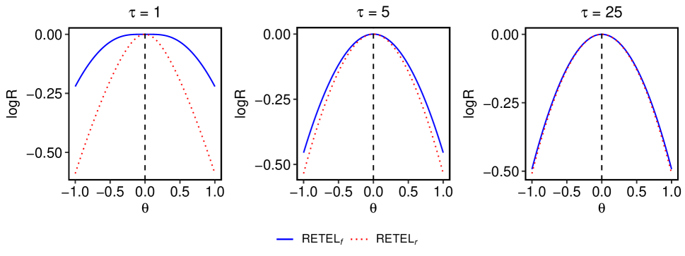
Figure 2: Plots of ${\log R_{RET}(\bm{\theta})}$ (solid blue lines) and ${\log\widetilde{R}_{RET}(\bm{\theta})}$ (dashed red lines) for the mean parameter with varying ${\tau_{n}}\in\{1,5,25\}$. Both versions of RETEL achieve their maximum at the single data point ${0}$ (vertical dashed line). Here, ${\mu_{n,\theta}}$ and ${\Sigma}_{n,\theta}$ are set to ${-\theta}$ and ${1}$, respectively. The difference between the two versions diminishes as ${\tau_{n}}$ increases.

Now, we establish that RETEL retains certain desirable asymptotic properties of EL and ETEL. We consider RETEL obtained from ${\bm{\lambda}_{RET}}$ in Equation 5. The following condition controls ${p_{n}(\bm{\theta},\bm{\lambda})}$ in Equation 4. The condition ensures the asymptotic stability of the regularization when it depends on ${n}$ and ${\bm{\theta}}$:

Condition 5.

${\tau_{n}}={O(\log n)}$; ${\bm{\mu}_{n,\bm{\theta}_{0}}}={\bm{\mu}}+{o_{P}(1)}$ for some ${\bm{\mu}}\in{\mathbb{R}^{p}}$; ${\bm{\Sigma}_{n,\bm{\theta}_{0}}}$ is positive definite for any ${n}$ with probability ${1}$; and ${\bm{\Sigma}_{n,\bm{\theta}_{0}}}={\bm{\Sigma}}+{o_{P}(1)}$ for some ${\bm{\Sigma}}\in\mathbb{R}^{p\times p}$.

Theorem 2.

Under Conditions 1, 2, 4, 2, 3 and 5, ${\log(R_{RET}(\bm{\theta}_{0})/\widetilde{R}_{RET}(\bm{\theta}_{0}))}=O_{P}({n^{-1/2}})$. Additionally, both ${-2\log R_{RET}(\bm{\theta}_{0})}$ and ${-2\log\widetilde{R}_{RET}(\bm{\theta}_{0})}$ converge in distribution to ${\chi^{2}_{p}}$.

As a consequence, the logarithms of the regularized methods are identical up to ${O_{P}(n^{-1/2})}$, and both methods exhibit Wilks’ theorem. For Bayesian inference, we can obtain the Bernstein–von Mises result for both versions of RETEL.

Condition 6.

The prior measure admits a density with respect to the Lebesgue measure. The density ${\pi}(\cdot)$ is continuous in ${\Theta}$ and is positive in a neighborhood of ${\bm{\theta}_{0}}$.

Condition 7.

For any ${\delta}>{0}$, there exists ${\epsilon}>{0}$ such that

$$P\left(\sup_{\left|\bm{\theta}-\bm{\theta}_{0}\right|>\delta}\frac{1}{n}\left(\log L_{RET}\left(\bm{\theta}\right)-\log L_{RET}\left(\bm{\theta}_{0}\right)\right)\leq-\epsilon\right)\to 1.$$

Condition 6 and Condition 7 are regularity conditions to establish the Bernstein–von Mises theorem for EL and ETEL (Chib et al., 2018; Yu & Bondell, 2023).

Theorem 3.

Under Conditions 1, 2, 4, 2, 3, 5, 6 and 7,

$$\sup_{\mathcal{B}}\left|\pi\left(n^{1/2}\left(\bm{\theta}-\bm{\theta}_{0}\right)\in\mathcal{B}\mathrel{}\middle|\mathrel{}\mathcal{D}_{n}\right)-N\left(\bm{0},\bm{\Omega}\right)\left(\mathcal{B}\right)\right|\to 0$$

in probability, where ${\pi(n^{1/2}(\bm{\theta}-\bm{\theta}_{0})\mid\mathcal{D}_{n})}$ is the posterior distribution of ${n^{1/2}(\bm{\theta}-\bm{\theta}_{0})}$ obtained from RETEL, and ${\mathcal{B}}\in{\Theta}$ denotes any Borel set.

This result implies that, when the moment constraints are correctly specified, the total variation distance between the posterior distribution of ${n^{1/2}(\bm{\theta}-\bm{\theta}_{0})}$ and ${N(\bm{0},\bm{\Omega})}$ tends to zero in probability.

4 Simulation

4.1 Posterior Coverage

Monahan & Boos (1992) proposed examining the validity of a pseudo-likelihood ${L(\theta)}$ based on the coverage probabilities of posterior intervals. For a parameter ${\theta}\in\mathbb{R}$, let ${\pi(\theta\mid x)}$ be the posterior density obtained using ${L(\theta)}$ with an absolutely continuous prior density ${\pi(\theta)}$ and observed data ${x}$. For this pseudo-likelihood to be valid by coverage, posterior intervals should provide correct coverage probabilities. In particular, when ${(X,\theta)}$ is generated from the Bayesian model, the random variable ${H}={\int_{-\infty}^{\theta}\pi(t\mid X)dt}$ should follow a uniform distribution ${U(0,1)}$. This approach has been adopted for EL by Lazar (2003) and Cheng & Zhao (2019).

To investigate the validity of RETEL for Bayesian inference, we begin by simulating a value of ${\theta}$ from a logistic distribution denoted as ${\textnormal{Logistic}(l,s)}$, where ${l}$ is the location parameter and ${s}$ is the scale parameter. Next, we generate ${n}$ observations from ${N(\theta,1)}$ and compute ${H}$ for the two versions of RETEL. Throughout the analysis, we employ ${p_{n}(\theta,\lambda)}$ in Equation 4 with ${\mu_{n,\theta}}={\overline{X}-\theta}$ and ${\Sigma_{n,\theta}}={1}$ for the univariate mean parameter ${\theta}$. For comparison purposes, we also compute ${H}$ using ETEL and AETEL. Keeping ${l}$ fixed at ${0}$, we repeat this procedure $10000$ times for each combination of ${n}\in{\{5,20,50,100\}}$, ${s}\in{\{1,5\}}$, and ${\tau_{n}}\in{\{1,\log n\}}$. We approximate the posterior distributions on a grid of ${\theta}$ values. Using the computed ${H}$ values, we conduct the Kolmogorov–Smirnov test to evaluate the uniformity of the distributions.

The resulting ${p}$-values are reported in Table 1, and Figure 3 displays the quantile-quantile plots for the distribution of ${H}$ versus ${U(0,1)}$ when ${n}={5}$, ${s}={5}$, and ${\tau_{n}}={1}$.

Table 1: ${p}$-values from the Kolmogorov–Smirnov test for uniformity.

		${\tau_{n}}={1}$		${\tau_{n}}={\log n}$
${n}$	${s}$	${\textnormal{RETEL}_{f}}$	${\textnormal{RETEL}_{r}}$	${\textnormal{RETEL}_{f}}$	${\textnormal{RETEL}_{r}}$	ETEL	AETEL
${5}$	${1}$	${<0.001}$	${0}$	${<0.001}$	${<0.001}$	${0}$	${0}$
	${5}$	${<0.001}$	${<0.001}$	${<0.001}$	${<0.001}$	${0}$	${0}$
${20}$	${1}$	${<0.001}$	${<0.001}$	${<0.001}$	${<0.001}$	${<0.001}$	${0.007}$
	${5}$	${<0.001}$	${<0.001}$	${0.001}$	${<0.001}$	${<0.001}$	${0.064}$
${50}$	${1}$	${0.262}$	${0.248}$	${0.303}$	${0.303}$	${0.221}$	${0.425}$
	${5}$	${0.360}$	${0.320}$	${0.414}$	${0.423}$	${0.303}$	${0.466}$
${100}$	${1}$	${0.428}$	${0.430}$	${0.417}$	${0.418}$	${0.364}$	${0.714}$
	${5}$	${0.363}$	${0.367}$	${0.389}$	${0.369}$	${0.323}$	${0.781}$

The plots highlight the differences in the tails of the distributions that are not apparent from the ${p}$-values alone. With a smaller sample size of ${n}={5}$, RETEL tends to show a closer conformity to ${U(0,1)}$ compared to ETEL and AETEL. The impact of a larger prior variance (${s}={5}$) and a larger ${p_{c}(\theta)}$ (${\tau_{n}}={\log n}$) becomes more apparent when ${n}={50}$. As the sample size increases, the differences between the posterior distributions of the methods become negligible. All of the methods provide an excellent approximation to the null distribution when ${n}$ is ${50}$ or more. We emphasize that the Kolmogorov–Smirnov tests are based on a sample of $10000$ replicates and so are able to pick up quite small departures from the uniform distribution. Additional plots for the full results are provided in Section 8 in the supplementary materials.

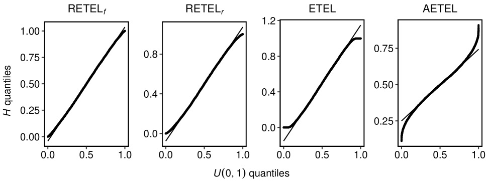
Figure 3: Quantile-quantile plots for the distribution of ${H}$ versus ${U(0,1)}$ when ${n}={5}$, ${s}={5}$, and ${\tau_{n}}={1}$. The light-tailed distribution from ETEL is due to the convex hull constraint. AETEL produces a heavier-tailed distribution than the others.

Next, we investigate the frequentist properties of the posterior intervals obtained from RETEL. We consider a true mean parameter value ${\theta_{0}}={0}$ and generate ${n}$ observations from ${N(0,1)}$. Using the logistic prior distribution described earlier, we compute ${95\%}$ posterior credible interval for ${\theta}$ using each of the four methods. This procedure is repeated $10000$ times for different combinations of ${n}\in{\{5,20,50,100\}}$, ${s}\in{\{0.5,1,5\}}$, and ${l}\in{\{0,2\}}$, while fixing ${\tau_{n}}$ at ${\log n}$. We then calculate the coverage rate and average length of the central credible intervals.

The results for ${l}={0}$ are presented in Table 2, where the prior mean matches the true parameter value. It can be seen that for all methods, as the sample size increases, the intervals become shorter and the coverage rates approach the target of ${95\%}$. As ${s}$ decreases, indicating stronger prior information on ${\theta}$ at ${0}$, higher coverage rates and shorter intervals are obtained. The differences between the methods are most pronounced when ${n}={5}$. The intervals obtained from ETEL exhibit significantly lower coverage rates compared to the other methods. AETEL produces the widest intervals with coverage rates higher than the nominal level. The wider intervals and departure from the nominal coverage rate are related to the boundedness problem of AEL, which arises due to the addition of one pseudo-observation (Emerson & Owen, 2009). On the other hand, RETEL yields coverage rates closer to the nominal level but features much shorter intervals compared to AETEL. Within RETEL, ${\textnormal{RETEL}_{f}}$ produces wider intervals with higher coverage rates than ${\textnormal{RETEL}_{r}}$, consistent with the findings from the plots in Figure 3.

Table 3 shows the results when ${l}={2}$, indicating a prior mean that is far from the true parameter value. In this case, the credible intervals tend to be wider with lower coverage rates. ETEL is relatively unaffected due to the convex hull constraint. However, the effect of different ${l}$ values is noticeable for the other methods. Particularly when ${n}={5}$ and ${s}={0.5}$, the strong prior shifts the intervals toward ${2}$. AETEL is the most affected, as its coverage rate is considerably lower than that of RETEL, even with wider intervals. To sum up, RETEL exhibits robust performance across various prior means and variances, demonstrating close-to-nominal posterior coverage rates with small sample sizes.

Table 2: Coverage rates (CR) and average lengths (Length) of ${95\%}$ credible intervals when ${l}={0}$.

$<{l}={0}>$		${\textnormal{RETEL}_{f}}$		${\textnormal{RETEL}_{r}}$		ETEL		AETEL
${n}$	${s}$	CR	Length	CR	Length	CR	Length	CR	Length
${5}$	${0.5}$	${95.9}$	${1.445}$	${94.4}$	${1.385}$	${79.2}$	${1.128}$	${100}$	${2.572}$
	${1}$	${94.1}$	${1.581}$	${92.4}$	${1.505}$	${77.8}$	${1.200}$	${100}$	${5.338}$
	${5}$	${93.2}$	${1.647}$	${91.3}$	${1.561}$	${77.2}$	${1.230}$	${100}$	${9.367}$
${20}$	${0.5}$	${94.2}$	${0.805}$	${94.0}$	${0.803}$	${93.1}$	${0.790}$	${96.3}$	${0.886}$
	${1}$	${93.6}$	${0.830}$	${93.4}$	${0.828}$	${92.4}$	${0.815}$	${96.0}$	${0.932}$
	${5}$	${93.3}$	${0.839}$	${93.1}$	${0.837}$	${92.2}$	${0.824}$	${96.1}$	${0.965}$
${50}$	${0.5}$	${94.8}$	${0.534}$	${94.8}$	${0.534}$	${94.5}$	${0.530}$	${95.8}$	${0.558}$
	${1}$	${94.5}$	${0.542}$	${94.5}$	${0.542}$	${94.2}$	${0.537}$	${95.4}$	${0.566}$
	${5}$	${94.5}$	${0.544}$	${94.4}$	${0.544}$	${94.1}$	${0.540}$	${95.3}$	${0.569}$
${100}$	${0.5}$	${94.8}$	${0.385}$	${94.8}$	${0.385}$	${94.6}$	${0.380}$	${95.2}$	${0.394}$
	${1}$	${94.7}$	${0.387}$	${94.7}$	${0.387}$	${94.4}$	${0.383}$	${95.1}$	${0.397}$
	${5}$	${94.6}$	${0.388}$	${94.6}$	${0.388}$	${94.3}$	${0.384}$	${95.1}$	${0.398}$

• Notes: CR is shown in percentage. The largest standard error of the lengths is ${0.005}$ when ${n}={5}$ and ${s}={5}$.

Table 3: Coverage rates (CR) and average lengths (Length) of ${95\%}$ credible intervals when ${l}={2}$.

$<{l}={2}>$		${\textnormal{RETEL}_{f}}$		${\textnormal{RETEL}_{r}}$		ETEL		AETEL
${n}$	${s}$	CR	Length	CR	Length	CR	Length	CR	Length
${5}$	${0.5}$	${86.3}$	${1.610}$	${85.3}$	${1.530}$	${73.2}$	${1.157}$	${80.0}$	${3.887}$
	${1}$	${92.6}$	${1.616}$	${90.8}$	${1.534}$	${76.9}$	${1.207}$	${100}$	${6.174}$
	${5}$	${93.1}$	${1.647}$	${91.3}$	${1.561}$	${77.2}$	${1.230}$	${100}$	${10.858}$
${20}$	${0.5}$	${91.6}$	${0.834}$	${91.4}$	${0.832}$	${90.7}$	${0.819}$	${94.2}$	${1.529}$
	${1}$	${93.0}$	${0.835}$	${92.9}$	${0.833}$	${92.1}$	${0.820}$	${96.6}$	${0.995}$
	${5}$	${93.3}$	${0.839}$	${93.1}$	${0.837}$	${92.2}$	${0.824}$	${96.2}$	${0.975}$
${50}$	${0.5}$	${93.5}$	${0.543}$	${93.4}$	${0.543}$	${93.3}$	${0.539}$	${94.4}$	${0.569}$
	${1}$	${94.3}$	${0.543}$	${94.3}$	${0.543}$	${94.1}$	${0.538}$	${95.2}$	${0.568}$
	${5}$	${94.5}$	${0.554}$	${94.5}$	${0.544}$	${94.1}$	${0.540}$	${95.3}$	${0.569}$
${100}$	${0.5}$	${94.2}$	${0.388}$	${94.2}$	${0.388}$	${94.0}$	${0.384}$	${94.7}$	${0.398}$
	${1}$	${94.5}$	${0.388}$	${94.4}$	${0.388}$	${94.2}$	${0.384}$	${95.0}$	${0.398}$
	${5}$	${94.6}$	${0.388}$	${94.6}$	${0.388}$	${94.3}$	${0.384}$	${95.1}$	${0.398}$

• Notes: CR is shown in percentage. The largest standard error of the lengths is ${0.006}$ when ${n}={20}$ and ${s}={0.5}$.

4.2 Expected Kullback–Leibler Divergence

The restricted posterior domain significantly affects Bayesian inference with EL and ETEL, especially when the sample size is small. In an example with only two observations, ${X_{1}}$ and ${X_{2}}$, where the interest is in the mean parameter ${\theta}$, the posterior domain shrinks to a singleton as ${|X_{1}-X_{2}|}$ decreases toward zero. This example illustrates a problematic aspect of EL and ETEL, where we have more definitive information on the parameter with fewer data.

More generally, consider a parametric model ${\mathcal{M}}={\{p(\bm{x}\mid\bm{\theta})\mid\bm{x}\in\mathcal{X},\bm{\theta}\in\Theta\}}$ and a prior density ${\pi(\bm{\theta})}$. The expected information obtained from observing ${\bm{x}}$ from ${\mathcal{M}}$ can be measured using the expected KL divergence:

$$I\left(\pi\mathrel{}\middle|\mathrel{}\mathcal{M}\right)=\int_{\mathcal{X}}D_{KL}\left(\pi\left(\cdot\mathrel{}\middle|\mathrel{}\bm{x}\right)\mathrel{}\middle\|\mathrel{}\pi\left(\cdot\right)\right)m\left(\bm{x}\right)d\bm{x},$$

where ${\pi(\bm{\theta}\mid\bm{x})}={\pi(\bm{\theta})p(\bm{x}\mid\bm{\theta})/m(\bm{x})}$ and ${m(\bm{x})}={\int_{\Theta}\pi(\bm{\theta})p(\bm{x}\mid\bm{\theta})d\bm{\theta}}$. Let ${I(\pi\mid\mathcal{M}_{n})}$ denote the expected information obtained from the set of observations ${\{\bm{x}_{1},\dots,\bm{x}_{n}\}}$. It is expected that ${I(\pi\mid\mathcal{M}_{n})}$ increases monotonically with ${n}$ (Mantovan & Todini, 2006). The following result, based on Berger et al. (2009, Theorem 3), illustrates this monotonicity property.

Proposition 4.

Let ${\mathcal{M}}={\{p(\bm{x}_{1},\bm{x}_{2}\mid\bm{\theta})\mid\bm{x}_{1}\in\mathcal{X},\bm{x}_{2}\in\mathcal{X},\bm{\theta}\in\Theta\}}$ be a model with a sufficient statistic ${\bm{t}}={\bm{t}(\bm{x}_{1},\bm{x}_{2})}\in{\mathcal{U}}$. Suppose ${\pi(\bm{\theta})}$ is a strictly positive and continuous prior on ${\Theta}$, where ${\pi(\bm{\theta}\mid\bm{x}_{1},\bm{x}_{2})}={\pi(\bm{\theta})p(\bm{x}_{1},\bm{x}_{2}\mid\bm{\theta})/m(\bm{x}_{1},\bm{x}_{2})}$ and ${m(\bm{x}_{1},\bm{x}_{2})}={\int_{\Theta}\pi(\bm{\theta})p(\bm{x}_{1},\bm{x}_{2}\mid\bm{\theta})d\bm{\theta}}<{\infty}$. Under Condition 1, if ${\int_{\mathcal{U}}p(\bm{t}\mid\bm{\theta})\log(p(\bm{t}\mid\bm{\theta})/p(\bm{t}\mid{\bm{\theta}}^{\prime}))dt}<{\infty}$ for any ${\bm{\theta}}\in{\Theta}$ and ${{\bm{\theta}}^{\prime}}\in{\Theta}$, then ${I(\pi\mid\mathcal{M}_{1})}\leq{I(\pi\mid\mathcal{M}_{2})}<{\infty}$.

Based on the above proposition, the approximate validity of a pseudo-likelihood for Bayesian inference can be evaluated by examining whether it preserves the monotonicity property.

To examine the performance of RETEL compared to EL and ETEL, we consider two independent experiments where we obtain independent observations, denoted as ${X_{ij}}$ for ${i}={1,2}$ and ${j}={1,\dots,n}$, from the following hierarchical model:

$$X_{ij}\mid\theta_{i} \sim N\left(\theta_{i},\sigma^{2}\right),$$

$$\theta_{i}\mid\mu \sim\textnormal{Cauchy}\left(\mu,\gamma\right),$$

$$\mu \sim N\left(0,\tau^{2}\right).$$

We assume fixed values of ${\sigma}={1}$, ${\gamma}={1}$, and ${\tau}={10}$. We use a variety of empirical likelihoods in place of the normal density for $X_{ij}$. Our main focus is on the marginal posterior distribution of ${\mu}$, with the density denoted by ${\pi(\mu\mid\mathcal{D}_{n})}$. Given the values of ${\theta_{1}}$ and ${\theta_{2}}$ with ${\Delta}={|\theta_{1}-\theta_{2}|}>{2}$, the Cauchy distribution for ${\theta_{1}}$ and ${\theta_{2}}$ yields two maximum likelihood estimates of ${\mu}$ given by ${(\theta_{1}+\theta_{2})/2}\pm{\sqrt{\Delta^{2}-1}}$ (Dharmadhikari & Joag-Dev, 1985). Consequently, when combined with the large standard deviation of the prior distribution for ${\mu}$, the restricted posterior domain of ${\theta_{1}}$ and ${\theta_{2}}$ from EL and ETEL leads to a bimodal marginal posterior distribution for ${\mu}$. This bimodality can potentially result in inflated values of ${I(\pi\mid\mathcal{M}_{n})}$ for EL and ETEL, particularly when ${n}$ is small.

The marginal likelihood, ${m({\bm{x}})}$, for the four methods cannot be computed analytically. Instead, we can observe that $I(\pi\mid\mathcal{M})$ can be expressed as:

$$I\left(\pi\mathrel{}\middle|\mathrel{}\mathcal{M}\right)=\int_{\Theta}\pi\left(\bm{\theta}\right)\left[\int_{\mathcal{X}}D_{KL}\left(\pi\left(\cdot\mathrel{}\middle|\mathrel{}\bm{x}\right)\mathrel{}\middle\|\mathrel{}\pi\left(\cdot\right)\right)p\left(\bm{x}\mid\bm{\theta}\right)d\bm{x}\right]d\bm{\theta},$$

where ${D_{KL}(\pi(\cdot\mid\bm{x})\|\pi(\cdot))}$ is computed with respect to ${\mu}$. Since our focus is on comparing ${I(\pi\mid\mathcal{M}_{n})}$ for the methods, we fix ${\theta_{1}}$ and ${\theta_{2}}$ at ${-3}$ and ${3}$, respectively. For each method and ${n}\in{\{2,4,6,8,10\}}$, we estimate the inner integrand of ${I(\pi\mid\mathcal{M}_{n})}$ through simulation using the following steps:

1. Generate ${X_{1j}}$ from ${N(-3,1)}$ and ${X_{2j}}$ from ${N(3,1)}$ for ${j}={1,\dots,n}$.

2. Generate $10000$ posterior samples of ${\theta_{1}}$, ${\theta_{2}}$, and ${\mu}$ with a random-walk Metropolis–Hastings algorithm.

3. Estimate ${\pi(\mu\mid\mathcal{D}_{n})}$ from the posterior samples and compute ${D_{KL}(\pi(\cdot\mid\mathcal{D}_{n})\ \|\ \pi(\cdot))}$ by numerical integration with adaptive quadrature.

4. Repeat Steps 1–3 $1000$ times and take the average of the estimates from Step 3.

Step 2 is implemented with two chains of length $5000$, ensuring that the potential scale reduction factor (Gelman & Rubin, 1992) remains below ${1.1}$ on average for each method. For the regularized methods, ${\tau_{n}}={1}$ is used when ${n=2}$, and ${\tau_{n}}={\log n}$ is used otherwise. We implement EL using the R package melt (Kim et al., 2024).

The results are summarized in Figure 4.

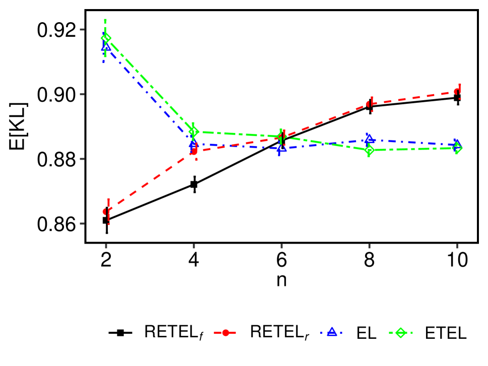
(a)

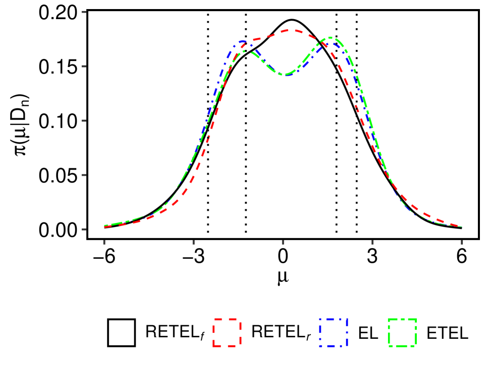
(b)

Figure 4: Plots of (a) the expected KL divergence (inner integrand) and (b) the marginal posterior density ${\pi(\mu\mid\mathcal{D}_{n})}$ with ${n}={2}$. The error bars in (a) represent plus or minus one standard error. The vertical dotted lines in (b) indicate the four realized data points.

In Figure 4(a), it can be seen that ${I(\pi\mid\mathcal{M}_{n})}$ is the smallest when ${n}={2}$ for ${\textnormal{RETEL}_{f}}$ (${0.861}$) and ${\textnormal{RETEL}_{r}}$ (${0.864}$), and it increases monotonically as the sample size grows. ${\textnormal{RETEL}_{r}}$ tends to produce slightly larger ${I(\pi\mid\mathcal{M}_{n})}$ compared to ${\textnormal{RETEL}_{f}}$. On the other hand, EL and ETEL attain the largest ${I(\pi\mid\mathcal{M}_{n})}$ when ${n}={2}$, with values of ${0.914}$ and ${0.917}$, respectively. The values of ${I(\pi\mid\mathcal{M}_{n})}$ decrease as the sample size and the range of the data increase. EL and ETEL do not exhibit an upward trend in ${I(\pi\mid\mathcal{M}_{n})}$ and, even as ${n}$ moves toward ${10}$, do not show a notable improvement. This discrepancy is caused by the strong bimodality of ${\pi(\mu\mid\mathcal{D}_{n})}$, as illustrated in Figure 4(b).

5 Application

We present an application of RETEL to the estimation of median 1989 income for four-person families by State in the USA. In the field of small area estimation (Ghosh & Rao, 1994; Rao, 2003), the state-level direct estimates provided by the Census Bureau based on the Current Population Survey data may not be sufficiently accurate for some states due to limited sample sizes. To address this issue, Bayesian methods have been proposed, which incorporate additional information or related auxiliary variables specific to these small areas (Fay & Herriot, 1979; Datta et al., 1996; Ghosh et al., 1996). In particular, EL has been applied to small area estimation in hierarchical Bayesian models (Chaudhuri & Ghosh, 2011; Chaudhuri et al., 2017; Jahan et al., 2022).

Let ${Y_{i}}$, ${i}={1,\dots,51}$, represent the direct estimate of the 1989 median income for four-person families in the ${i}$th state, including the District of Columbia. We also consider the direct estimate of the 1979 median income, denoted by ${X_{1i}}$, as an auxiliary variable. Additionally, following Chung et al. (2019), we incorporate the adjusted census median income denoted by ${X_{2i}}$, where ${X_{2i}}={(\textnormal{PCI}_{i,1989}/\textnormal{PCI}_{i,1979})X_{1i}}$. Here, ${\textnormal{PCI}_{i,1979}}$ and ${\textnormal{PCI}_{i,1989}}$ refer to per capita income from the Bureau of Economic Analysis in 1979 and 1989, respectively. All variables are standardized to ensure numerical stability and facilitate illustration.

Similar to the generalized linear model approach of Chaudhuri & Ghosh (2011), we assume that the ${Y_{i}}$ are conditionally independent given ${\theta_{i}}$. Specifically, we assume:

$$\textnormal{E}\left[Y_{i}\mid\theta_{i}\right]=\theta_{i}, \quad\textnormal{Var}\left[Y_{i}\mid\theta_{i}\right]=V_{i},$$

$$\theta_{i}\mid\bm{\beta},\sigma^{2} \overset{\textnormal{ind}}{\sim}N\left(\bm{X}_{i}^{\top}\bm{\beta},\sigma^{2}\right),$$

$$\bm{\beta}\mid\sigma^{2} \sim N\left(\bm{\beta}_{0},g\sigma^{2}\left(\bm{X}^{\top}\bm{X}\right)^{-1}\right),$$

$$\sigma^{2} \sim\pi\left(\sigma^{2}\mathrel{}\middle|\mathrel{}\mathcal{D}_{n}\right)\propto\frac{1}{\sigma^{2}}.$$

Here, ${\bm{\beta}}={(\beta_{1},\beta_{2})}$, ${\bm{X}_{i}}={(X_{1i},X_{2i})}$, and ${\bm{X}}$ is the matrix with the ${i}$th row given by ${\bm{X}_{i}^{\top}}$. The sampling variance ${V_{i}}$ is set to ${1}$. We adopt the ${g}$-prior of Zellner (1988) for ${\bm{\beta}}$ with ${\bm{\beta}_{0}}={(\bm{X}^{\top}\bm{X})^{-1}\bm{X}^{\top}\bm{Y}}$ and ${g}={0.1}$, where ${\bm{Y}}={(Y_{1},\dots,Y_{51})}$. For the likelihood function, we use ${\textnormal{RETEL}_{f}}$, ${\textnormal{RETEL}_{r}}$, EL, and ETEL with the bivariate estimating function ${(Y_{i}-\theta_{i},(Y_{i}-\theta_{i})^{2}/V_{i}-1)}$.

For each method, we use a random-walk Metropolis–Hastings algorithm to draw posterior samples of ${\bm{\theta}}$, ${\bm{\beta}}$, and ${\sigma^{2}}$ from four chains, each of length $250000$. The regularized versions employ ${\mu_{n,\bm{\theta}}}={n^{-1}\sum_{i=1}^{n}\bm{g}(Y_{i},\bm{\theta})}$, ${\bm{\Sigma}_{n,\bm{\theta}}}={(n-1)^{-1}\sum_{i=1}^{n}\bm{g}(Y_{i},\bm{\theta}){\bm{g}(Y_{i},\bm{\theta})}^{\top}}$, and ${\tau_{n}}={\log n}$, where ${n}={51}$. The maximum potential scale reduction factor of all the methods is ${1.0119}$ for ${\bm{\theta}}$, ${1.0006}$ for ${\bm{\beta}}$, and ${1.0137}$ for ${\sigma^{2}}$. We compute the ${95\%}$ posterior credible interval for each ${\theta_{i}}$ and use the posterior median ${\widehat{\theta}_{i}}$ as an estimate for ${Y_{i}}$. The performance of the methods is evaluated using the following metrics: average absolute deviation (AAD) ${n^{-1}\sum_{i=1}^{n}|\widehat{\theta}_{i}-Y_{i}|}$, average absolute relative deviation (AARD) ${n^{-1}\sum_{i=1}^{n}|(\widehat{\theta}_{i}-Y_{i})/Y_{i}|}$, average squared deviation (ASD) ${n^{-1}\sum_{i=1}^{n}(\widehat{\theta}_{i}-Y_{i})^{2}}$, and average squared relative deviation (ASRD) ${n^{-1}\sum_{i=1}^{n}((\widehat{\theta}_{i}-Y_{i})/Y_{i})^{2}}$.

Table 4 provides the summary. The results show that RETEL demonstrates improvement over EL and ETEL, exhibiting smaller deviations in all metrics and providing more accurate estimates. Although RETEL has slightly longer intervals compared to EL and ETEL, ${\textnormal{RETEL}_{r}}$ performs the best among the methods in terms of accuracy. On the other hand, EL and ETEL exhibit nearly equivalent performances, aligning with the findings in Chaudhuri & Ghosh (2011).

Table 4: Comparison of the accuracy of estimates of ${\bm{\theta}}$ from the four methods. The average length of the ${51}$ credible intervals is added for each method (Length).

Method	AAD	AARD	ASD	ASRD	Length
${\textnormal{RETEL}_{f}}$	${0.278}$	${0.911}$	${0.111}$	${3.982}$	${3.754}$
${\textnormal{RETEL}_{r}}$	${0.272}$	${0.900}$	${0.109}$	${3.831}$	${3.781}$
EL	${0.280}$	${0.947}$	${0.112}$	${4.587}$	${3.755}$
ETEL	${0.279}$	${0.942}$	${0.115}$	${4.696}$	${3.729}$

6 Discussion

Bayesian methods are fundamentally based on probability, with inference proceeding from the prior distribution to the posterior distribution via conditioning on the observed data. Bayesian versions of EL and ETEL place a prior distribution on a finite number of features of a nonparametric (and hence infinite dimensional) distribution and regard the remainder of the distribution itself as a nuisance parameter. The lack of a full probability model prevents one from integrating over the nuisance parameter. EL and ETEL replace the integration with a maximization, and this replacement produces artifacts that clash with known properties that all Bayesian methods must have.

The most striking departure from Bayesian behavior is the zeroing out of regions of the parameter space as one moves from prior distribution to posterior distribution, with the expectation that, as more data are collected, the zeroed out regions will reappear and be assigned positive probability. These regions concern the main parameters of interest–those that are represented by the estimating equations that give rise to EL and ETEL. The regions and behavior follow from the convex hull constraint. Another feature of Bayesian methods (and most other statistical methods) is that the data are the data. An observation, ${\bm{X}_{i}}$, may come from a distribution that depends on an unknown parameter ${\bm{\theta}}$, but ${\bm{X}_{i}}$ is not allowed to differ for different values of ${\bm{\theta}}$. Methods previously proposed to handle the convex hull constraint, such as AEL and AETEL, rely on pseudo-data that change with the parameter.

This paper has investigated a suite of methods to deal with the convex hull constraint without the need to invoke parameter-dependent pseudo-data. The first step was the development of WETEL as an extension of AEL and AETEL. WETEL accommodates fractional observations and reduces the dependence of pseudo-data on the parameter, allowing for a massive expansion of the convex hull while aligning the pseudo-data more closely with the observed data. As a subsequent step, WETEL leads to the regularization technique of RETEL by passing to a limit where pseudo-data are added in a particular way. We also provided a distinct derivation of RETEL as the solution to a KL divergence optimization problem involving a mixture of the empirical distribution and a continuous exponential family distribution.

The likelihood ratios from RETEL compare the constrained regularized likelihood to the unconstrained regularized likelihood. This is implicit in Equations 7 and 8. In essence, RETEL replaces the empirical distribution with a regularized empirical distribution before considering tilts that match constraints. This stabilizes the results, particularly for smaller sample sizes. It also appears to produce a posterior distribution that is less pathological and more amenable to traditional sampling techniques for model fitting. We showed that RETEL retains the desirable properties of EL and ETEL such as Wilks’ and Bernstein–von Mises’ theorems. The simulation and data analysis demonstrated that RETEL exhibits improved finite sample performance compared to EL and ETEL for Bayesian inference. Overall, our findings highlight the effectiveness of RETEL as a pseudo-likelihood for Bayesian inference in overcoming the convex hull constraint of EL and ETEL.

There are a number of reasons to replace integration in a Bayesian model with maximization. In addition to handling the nuisance parameter, maximization can be much quicker than integration. We suspect that an appropriate regularization in RETEL will bring the maximized version of the problem closer to a genuine Bayesian solution. This is a direction for future research. Another promising direction involves investigating whether RETEL retains the robust higher-order asymptotic properties of ETEL. Jing & Wood (1996) showed that ETEL is not Bartlett correctable. Schennach (2007) showed that the ETEL has robust higher-order asymptotic properties under model misspecification compared to the EL estimator. Chib et al. (2018) established Bernstein–von Mises results for ETEL under model misspecification. Further research is needed to determine the extent to which these properties hold for RETEL.

Supplementary Materials

The supplementary materials contain technical proofs and plots from simulations.

Funding

This work was supported by the National Science Foundation under Grants No. SES-1921523 and DMS-2015552.

References

- (1)
- Artstein & Wets (1995) Artstein, Z. & Wets, R. J.-B. (1995), ‘Consistency of minimizers and the SLLN for stochastic programs’, Journal of Convex Analysis 2, 1–17.
- Bartolucci (2007) Bartolucci, F. (2007), ‘A penalized version of the empirical likelihood ratio for the population mean’, Statistics & Probability Letters 77, 104–110.
- Berger et al. (2009) Berger, J. O., Bernardo, J. M. & Sun, D. (2009), ‘The formal definition of reference priors’, The Annals of Statistics 37, 905–938.
- Chang et al. (2018) Chang, J., Tang, C. Y. & Wu, T. T. (2018), ‘A new scope of penalized empirical likelihood with high-dimensional estimating equations’, The Annals of Statistics 46, 3185–3216.
- Chaudhuri & Ghosh (2011) Chaudhuri, S. & Ghosh, M. (2011), ‘Empirical likelihood for small area estimation’, Biometrika 98, 473–480.
- Chaudhuri et al. (2017) Chaudhuri, S., Mondal, D. & Yin, T. (2017), ‘Hamiltonian Monte Carlo sampling in Bayesian empirical likelihood computation’, Journal of the Royal Statistical Society, Series B 79, 293–320.
- Chen et al. (2008) Chen, J., Variyath, A. M. & Abraham, B. (2008), ‘Adjusted empirical likelihood and its properties’, Journal of Computational and Graphical Statistics 17, 426–443.
- Cheng & Zhao (2019) Cheng, Y. & Zhao, Y. (2019), ‘Bayesian jackknife empirical likelihood’, Biometrika 106, 981–988.
- Chib et al. (2018) Chib, S., Shin, M. & Simoni, A. (2018), ‘Bayesian estimation and comparison of moment condition models’, Journal of the American Statistical Association 113, 1656–1668.
- Chung et al. (2019) Chung, H. C., Datta, G. S. & Maples, J. (2019), Estimation of Median Incomes of the American States: Bayesian Estimation of Means of Subpopulations, Springer-Verlag, pp. 505–518.
- Corcoran (1998) Corcoran, S. A. (1998), ‘Bartlett adjustment of empirical discrepancy statistics’, Biometrika 85, 967–972.
- Cover & Thomas (2006) Cover, T. M. & Thomas, J. A. (2006), Elements of Information Theory, Wiley-Interscience.
- Cressie & Read (1984) Cressie, N. & Read, T. R. (1984), ‘Multinomial goodness-of-fit tests’, Journal of the Royal Statistical Society, Series B 46, 440–464.
- Datta et al. (1996) Datta, G., Ghosh, M., Nangia, N. & Natarajan, K. (1996), Estimation of median income of four-person families: a Bayesian approach, in ‘Bayesian analysis in statistics and econometrics: essays in honor of Arnold Zellner’, pp. 129–140.
- Dharmadhikari & Joag-Dev (1985) Dharmadhikari, S. & Joag-Dev, K. (1985), ‘Examples of nonunique maximum likelihood estimators’, The American Statistician 39, 199–200.
- DiCiccio et al. (1991) DiCiccio, T. J., Hall, P. & Romano, J. (1991), ‘Empirical likelihood is Bartlett-correctable’, The Annals of Statistics 19, 1053–1061.
- Dupačová (1992) Dupačová, J. (1992), ‘Epi-consistency in restricted regression models: The case of a general convex fitting function’, Computational Statistics & Data Analysis 14, 417–425.
- Dupačová & Wets (1988) Dupačová, J. & Wets, R. J.-B. (1988), ‘Asymptotic behavior of statistical estimators and of optimal solutions of stochastic optimization problems’, The Annals of Statistics 16, 1517–1549.
- Efron (1981) Efron, B. (1981), ‘Nonparametric standard errors and confidence intervals’, Canadian Journal of Statistics 9, 139–158.
- Emerson & Owen (2009) Emerson, S. C. & Owen, A. B. (2009), ‘Calibration of the empirical likelihood method for a vector mean’, Electronic Journal of Statistics 3, 1161–1192.
- Fay & Herriot (1979) Fay, R. E. & Herriot, R. A. (1979), ‘Estimates of income for small places: An application of James–Stein procedures to census data’, Journal of the American Statistical Association 74, 269–277.
- Gelman & Rubin (1992) Gelman, A. & Rubin, D. B. (1992), ‘Inference from iterative simulation using multiple sequences’, Statistical Science 7, 457–472.
- Ghosh et al. (1996) Ghosh, M., Nangia, N. & Kim, D. H. (1996), ‘Estimation of median income of four-person families: A Bayesian time series approach’, Journal of the American Statistical Association 91, 1423–1431.
- Ghosh & Rao (1994) Ghosh, M. & Rao, J. N. K. (1994), ‘Small area estimation: An appraisal’, Statistical Science 9, 55–76.
- Glenn & Zhao (2007) Glenn, N. & Zhao, Y. (2007), ‘Weighted empirical likelihood estimates and their robustness properties’, Computational Statistics & Data Analysis 51, 5130–5141.
- Grendár & Judge (2009) Grendár, M. & Judge, G. (2009), ‘Empty set problem of maximum empirical likelihood methods’, Electronic Journal of Statistics pp. 1542–1555.
- Hainmueller (2012) Hainmueller, J. (2012), ‘Entropy balancing for causal effects: A multivariate reweighting method to produce balanced samples in observational studies’, Political Analysis 20, 25–46.
- Hjort et al. (2018) Hjort, N. L., McKeague, I. W. & van Keilegom, I. (2018), ‘Hybrid combinations of parametric and empirical likelihoods’, Statistica Sinica 28, 2389–2407.
- Jahan et al. (2022) Jahan, F., Kennedy, D. W., Duncan, E. W. & Mengersen, K. L. (2022), ‘Evaluation of spatial Bayesian empirical likelihood models in analysis of small area data’, PLOS ONE 17, 1–27.
- Jing & Wood (1996) Jing, B.-Y. & Wood, A. T. A. (1996), ‘Exponential empirical likelihood is not Bartlett correctable’, The Annals of Statistics 24, 365–369.
-
Kim (2023)
Kim, E. (2023), melt: Multiple Empirical Likelihood Tests.
R package version 1.10.0.
https://CRAN.R-project.org/package=melt -
Kim (2024)
Kim, E. (2024), retel: Regularized Exponentially Tilted Empirical Likelihood.
R package version 0.1.0.
https://CRAN.R-project.org/package=retel - Kim et al. (2024) Kim, E., MacEachern, S. N. & Peruggia, M. (2024), ‘melt: Multiple empirical likelihood tests in R’, Journal of Statistical Software 108(5), 1–33.
- King & Wets (1991) King, A. J. & Wets, R. J.-B. (1991), ‘Epi‐consistency of convex stochastic programs’, Stochastics and Stochastic Reports 34, 83–92.
- Lazar (2003) Lazar, N. A. (2003), ‘Bayesian empirical likelihood’, Biometrika 90, 319–326.
- Leng & Tang (2012) Leng, C. & Tang, C. Y. (2012), ‘Penalized empirical likelihood and growing dimensional general estimating equations’, Biometrika 99, 703–716.
- Liu & Chen (2010) Liu, Y. & Chen, J. (2010), ‘Adjusted empirical likelihood with high-order precision’, The Annals of Statistics 38, 1341–1362.
- Mantovan & Todini (2006) Mantovan, P. & Todini, E. (2006), ‘Hydrological forecasting uncertainty assessment: Incoherence of the GLUE methodology’, Journal of Hydrology 330, 368–381.
- Monahan & Boos (1992) Monahan, J. F. & Boos, D. D. (1992), ‘Proper likelihoods for Bayesian analysis’, Biometrika 79, 271–278.
- Newey & Smith (2004) Newey, W. K. & Smith, R. J. (2004), ‘Higher order properties of GMM and generalized empirical likelihood estimators’, Econometrica 72, 219–255.
- Owen (1988) Owen, A. B. (1988), ‘Empirical likelihood ratio confidence intervals for a single functional’, Biometrika 75, 237–249.
- Qin (1994) Qin, J. (1994), ‘Semi-empirical likelihood ratio confidence intervals for the difference of two sample means’, Annals of the Institute of Statistical Mathematics 46, 117–126.
- Qin & Lawless (1994) Qin, J. & Lawless, J. (1994), ‘Empirical likelihood and general estimating equations’, The Annals of Statistics 22, 300–325.
- Rao (2003) Rao, J. N. K. (2003), Small Area Estimation, Wiley-Interscience.
- Rockafellar & Wets (2009) Rockafellar, R. T. & Wets, R. J.-B. (2009), Variational analysis, Springer-Verlag.
- Schennach (2005) Schennach, S. M. (2005), ‘Bayesian exponentially tilted empirical likelihood’, Biometrika 92, 31–46.
- Schennach (2007) Schennach, S. M. (2007), ‘Point estimation with exponentially tilted empirical likelihood’, The Annals of Statistics 35, 634–672.
- Smith (1997) Smith, R. J. (1997), ‘Alternative semi‐parametric likelihood approaches to generalised method of moments estimation’, The Economic Journal 107, 503–519.
- Sueishi (2022) Sueishi, N. (2022), ‘Large sample justifications for the Bayesian empirical likelihood’, Econometric Theory 0, 1–31.
- Tang & Leng (2010) Tang, C. Y. & Leng, C. (2010), ‘Penalized high-dimensional empirical likelihood’, Biometrika 97, 905–920.
- Tsao & Wu (2013) Tsao, M. & Wu, F. (2013), ‘Empirical likelihood on the full parameter space’, The Annals of Statistics 41, 2176–2196.
- Wets (1974) Wets, R. J.-B. (1974), ‘Stochastic programs with fixed recourse: The equivalent deterministic program’, SIAM Review 16, 309–339.
- Yiu et al. (2020) Yiu, A., Goudie, R. J. B. & Tom, B. D. M. (2020), ‘Inference under unequal probability sampling with the Bayesian exponentially tilted empirical likelihood’, Biometrika 107, 857–873.
- Yu & Bondell (2023) Yu, W. & Bondell, H. D. (2023), ‘Variational Bayes for fast and accurate empirical likelihood inference’, Journal of the American Statistical Association 0, 1–13.
- Zellner (1988) Zellner, A. (1988), ‘Bayesian analysis in econometrics’, Journal of Econometrics 37, 27–50.
- Zhu et al. (2009) Zhu, H., Zhou, H., Chen, J., Li, Y., Lieberman, J. & Styner, M. (2009), ‘Adjusted exponentially tilted likelihood with applications to brain morphology’, Biometrics 65(3), 919–927.