1]\orgdivDepartment of Physics, \orgnameUniversity of Belgrade, \orgaddress\streetStudentski Trg 12-16, \cityBelgrade, \postcode11000, \countrySerbia
2]\orgdivCenter for the Study of Complex Systems, \orgnameInstitute of Physics Belgrade, \orgaddress\streetPregrevica 118, \cityBelgrade, \postcode11080, \countrySerbia
Thermodynamic formalism and anomalous transport in 1D semiclassical Bose-Hubbard chain
Abstract
We analyze the time-dependent free energy functionals of the semiclassical one-dimensional Bose-Hubbard chain. We first review the weakly chaotic dynamics and the consequent early-time anomalous diffusion in the system. The anomalous diffusion is robust, appears with strictly quantized coefficients, and persists even for very long chains (more than hundred sites), crossing over to normal diffusion at late times. We identify fast (angle) and slow (action) variables and thus consider annealed and quenched partition functions, corresponding to fixing the actions and integrating over the actions, respectively. We observe the leading quantum effects in the annealed free energy, whereas the quenched energy is undefined in the thermodynamic limit, signaling the absence of thermodynamic equilibrium in the quenched regime. But already the leading correction away from the quenched regime reproduces the annealed partition function exactly. This encapsulates the fact that in both slow- and fast-chaos regime both the anomalous and the normal diffusion can be seen (though at different times).
keywords:
Bose-Hubbard model, Quantum chaos, Anomalous transport, Thermodynamic formalism, Quenched disorder1 Introduction
The vast and interesting phenomenology of cold atom systems [1], the universal behavior of theoretical models such as the SYK model [2, 3, 4], and novel indicators of quantum dynamics such as OTOC [5, 6, 7, 8] and Krylov complexity [9, 10, 11, 12] have led to resurgent interest in quantum chaos. The Bose-Hubbard model is an example of a cold-atom system which is nonintegrable and exhibits quantum chaos [13, 14, 15, 16, 17, 18, 19]. A convenient property of this model is also that it has a classical limit [20, 21], facilitating the comparisons of classical and quantum dynamics.
Our goal is to study the interplay between (weak) chaos and dynamics of the system, in particular the transport which we have previously found to be strongly anomalous [19]. Anomalous transport is expected in weakly chaotic systems [22, 23], however in our case it has strictly integer exponents and , where is a non-negative integer. This is surprising as the anomalous exponents are usually fractional [23]. We have found that anomalous diffusion holds even for enormous chains, with sites. This is also surprising as we expect the relative measure of stable regions in phase space to diminish to zero in the limit, leading to strong chaos and normal diffusion.
In this work we look at weak chaos and anomalous transport from the thermodynamic point of view: we calculate the partition function and free energy of the system. Since the dynamics exhibits timescale separation into fast and slow variables, it is natural to consider two possible definitions of the partition function: integrate over both fast and slow variables (annealed partition function) or solely over the fast variables, fixing the slow ones (quenched partition function). With some hindsight, we can say that the two approaches correspond to different epochs in the evolution of the system: early-time anomalous diffusion versus long-time normal diffusion regime. Nevertheless, the complete picture is still evasive, as we can only evaluate the free energies at leading order, in a very crude approximation.
2 The model
We consider a one-dimensional Bose-Hubbard chain with sites, whose Hamiltonian is given by:
| (1) |
where is the hopping parameter, is the on-site Coulomb repulsion, are bosonic creation and annihilation operators, is the occupation number of the site and is the chemical potential. We do not impose periodic boundary conditions, so for .
We are interested in the semiclassical regime, i.e. when the number of particles goes to infinity while the number of sites stays fixed. The semiclassical Hamiltonian is obtained by introducing new variables: [20, 21, 19]. The commutator of new variables vanishes as and the Hamiltonian becomes classical, with rescaled Coulomb repulsion parameter and the number-conservation constraint . Finally, we introduce the action-angle variables and the Hamiltonian in the these coordinates reads:
| (2) |
Actions have a very simple and natural interpretation: they are the occupation numbers for each site, which is seen also from the constraint . As usual in weakly nonintegrable systems, the actions evolve slowly whilst the angles change rapidly. From Eq. (2) we arrive at the equations of motion:
| (3) | |||
| (4) |
Equations of motions are nonlinear which tells us that the system is nonintegrable. In special cases and the system becomes integrable. In general, low/high ratio corresponds to tight/weak binding regime, leading to the superfluid and Mott insulator regimes respectively [24, 20, 25].111Since the model is one-dimensional there are no phase transitions but we can speak of two regimes separated by a crossover.
3 Chaos and transport
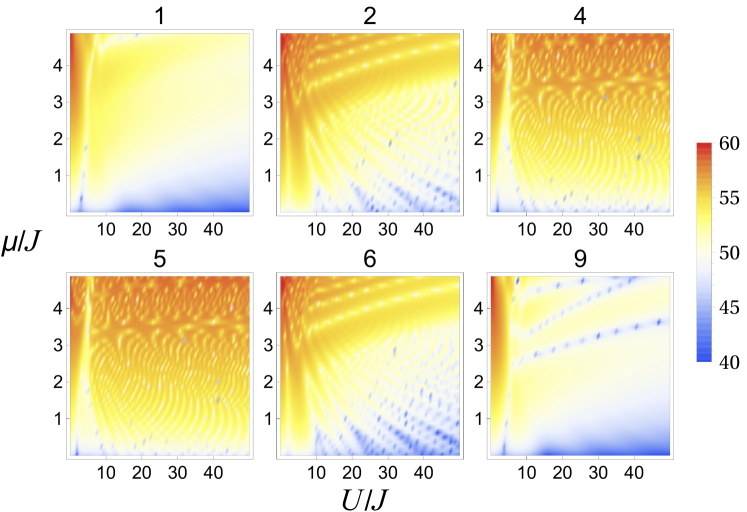
In [19] we have calculated the Lyapunov exponents in order to characterize chaos. What we observe is that the sites with a large initial occupation number in general have largest Lyapunov exponents which do not change significantly with the growth of ; initially empty sites have the lowest Lyapunov exponents (Fig. 1). To further corroborate this we have also computed the Lyapunov exponent for varying and (Figs. 1 and 2), and found that, for strongly chaotic sites, the strength of chaos is almost independent of the system parameters. On the other hand, the initial conditions, i.e. the initial occupation numbers are crucial for the development of chaos.

We now move to the central result of our work so far. We consider a population of orbits in phase space with initial conditions distributed, e.g. as a Gaussian peaked at the point . For strongly chaotic systems we expect to find diffusion in the space of actions [26, 22]. We inspect it by calculating:
| (5) |
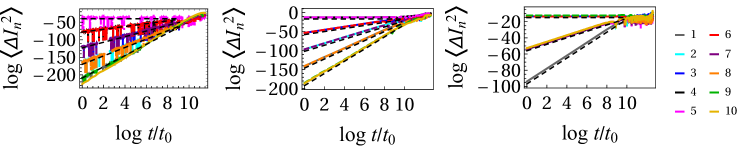
for the observed population of orbits. We observe strong superdiffusion of the action variables, that is where . The only instances where this strongly anomalous diffusion is absent are the initially filled sites, which show no diffusion at all, i.e. they have . The coefficients are completely independent of the parameters of the system (, ). They are thus a characteristic of the model and depend solely on the geometry of the initial conditions.
In general the anomalous exponent equals , with a positive integer which equals the distance of the given site from the nearest initially filled site. In particular this also means that initially filled sites have the exponent . This is observed for almost all initial conditions, and for all ranges of parameters. In special cases, when the initial conditions are sufficiently complicated and many sites are initially partially filled with similar fillings, we also observe exponents equal to with integer . In Fig. 3 we show the typical case, when the exponents equal .
The origin of anomalous coefficients is very hard to understand [27, 23], but according to Zaslavsky [28] we can give a crude explanation, at least for the case . For this case, we can use the non-resonant perturbation theory where the perturbed Hamiltonian has the form of a pendulum Hamiltonian [19]. It turns out that the period of oscillations of the pendulum is proportional to the square root of the action: . Rescaling these quantities by some factors and , we find that the system stays invariant if . Extending this to sites one derives: . From the Renormalization Group of kinetics formalism [28, 22, 23], the diffusion coefficients are given as:
| (6) |
just like in the numerics.
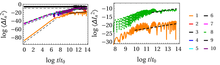
Finally, everything we have said so far of anomalous transport remains true up to some (large) time . Indeed we would expect that at some point the system approaches some form of thermal equilibrium, even if the time to reach it can be very large. This is indeed observed in our numerical calculations. In Fig. 4 we can follow how anomalous diffusion becomes normal, with , for sufficiently large times.
4 Thermodynamics
We have seen that at long times the system reaches the normal diffusion regime. We are still not sure about the meaning of the anomalous regime: is it a pre-thermalized regime or a regime which captures long-distance correlations and thus is not hydrodynamic. In order to shed some light on this, we calculate the partition functions of the system. The catch is that in principle we need to compute them as a function of time, i.e. for the evolving values of the variables – this is necessary because our system is strongly out-of-equilibrium. Instead of integrating over all possible exact trajectories which is a hopeless task we will use two drastic approximations. Of course, it would be preferable to apply the usual formalism of non-equilibrium thermodynamics but for now we just want to have some indication of what is happening in the simplest possible approach.
The are now two possible limits: annealed and quenched. Annealed partition function is obtained when treating all the variables equally, that is, we integrate over the whole phase space, both actions and angles. But since the angles are fast-winding variables and the actions change slowly, it also make sense to consider the quenched approximation where we freeze the actions at their initial values and then integrate the logarithm of the partition function for the angles to arrive at the quenched free energy.
4.1 Annealed partition function
By definition, the partition function is given as:
| (7) |
where indicates integration over all variables and is the inverse temperature. We first perform the integration over the angles:
| (8) |
where is the modified Bessel function of zeroth order. This result follows from the known integral:
| (9) |
Exact integration over the actions in (8) can only be done in the limit, representing the Bessel functions as a power series. The result is given by:
| (10) |
In the above we have denoted , . This is essentially an expansion in , therefore although the annealed approximation would be expected to work only in the superfluid regime where the actions evolve faster than in the Mott regime (though still slower than the angles), in fact we can also write a controlled expansion which remains valid into the Mott regime too. In this regime it makes sense to only keep the zeroth and first term in the above expansion:
| (11) |
From the above relation we can directly obtain the thermodynamic energy and the heat capacity:
| (12) |
Therefore, in the annealed regime the system behaves thermodynamically as an ideal gas – the expressions (12) are just the consequence of the equipartition theorem, with the twist that the degrees of freedom are not enumerated by particles but by sites (each site contributes exactly to the internal energy). In this case the normal diffusion regime (which we observe at very late times) is naturally expected. For later comparison to the quenched case, we also give the free energy in the annealed regime (also at the first order in the expansion (10)):
| (13) |
4.2 Quenched free energy
For the quenched calculation we only integrate over the angles, calculate the logarithm of the outcome (i.e., the free energy) and then average it over the actions, arriving at the following integral:
| (14) |
This integral can be computed exactly, even when does not go to infinity. This is done by introducing the hyperspherical coordinates. We present only the final result:
| (15) | |||||
Above we define (for the previously defined we thus have ). For some intuitive insight we only take the first term in this expansion, i.e. the term with :222The radius of convergence of equation (15) is quite difficult to analyze, as the last term in the sum behaves as a product of Bessel functions suppressed by a polynomial with a leading term being proportional to . We expect it to diverge for a wide range of the parameter. When , we have a controlled approximation leading to results in equations (16) and (17).
| (16) |
From here we derive the internal energy and heat capacity:
| (17) |
We see a few surprising things in this analysis. First, there is the factor of in the quenched quantities which appears from the integration over the -dimensional sphere (which does not happen in the annealed case). Because of this the strict thermodynamic limit predicts zero free energy, i.e. the breakdown of thermodynamics. This basically means that in the quenched regime there is no thermal equilibrium.
Assuming that the above results make some sense for finite , we note that the heat capacity now decreases with temperature as , which is unexpectedly consistent with the results of [29], obtained without assuming the semiclassical approximation. Therefore, the quenched approximation might be able to ”reproduce” the results of the quantum regime – the quenching of the slow variables essentially mimics the influence of quantum corrections.
4.3 Path integral approach
Since both annealed and quenched free energies capture only special limits, we will also calculate the partition function in the full path integral formalism – but for that of course we again need to resort to approximations, reducing the dynamics to linearized oscillations around the equilibrium points. It will turn out that taking into account even small linearized oscillations of the actions already bridges the gap between the annealed and the quenched regime. The Lagrangian of the system is given by Legendre transformation of the Hamiltonian:
| (18) |
The above result is interesting: the Lagrangian is formally given by the sum of ”kinetic energies” of non-interacting point particles of mass . Moreover, the Lagrangian only depends on the Coulomb repulsion , and not on , so we have a non-interacting Lagrangian with a single scale.333Of course, the canonical transformations from the original variables to depend on both and hence the system in fact knows of all the parameters as it has to be. What is more, this also holds for the rectangular and cubic lattice. Now we find the Euclidean action and the partition function (where we do not explicitly write out the normalization ):
| (19) |
where are the variables describing the dynamics of the system around some equilibrium point (below we define in detail). The first approximation for the solution for the actions is Therefore we can define the positions of the actions so that . The path integral is now calculated by perturbing the classical trajectory by some . It can easily be shown that
| (20) |
Substituting the integral becomes:
| (21) |
In the first approximation the result is:
| (22) |
The outcome (and the thermodynamics) is the same as for the annealed partition function. However, the starting assumptions and thus the interpretation are not the same:
-
1.
The annealed partition function is obtained by integrating the statistical weights with the full nonlinear Hamiltonian over the whole phase space, essentially assuming that both the actions and the angles are ergodic and explore the whole phase space during their evolution, for any .
-
2.
On the other hand, in the path integral calculation we introduce just the leading, linear correction to the opposite, quenched regime as we model the evolution of the actions by linear oscillations around fixed positions – and we have a formally noninteracting Lagrangian. Of course, the interactions are hidden in the constraints between the variables which would show up if we did not take a linearized approximation for the fluctuations .
Therefore, there is a tradeoff: ergodic/annealed dynamics for the full interacting system captures the same thermodynamic regime as the near-quenched dynamics but in the linearized approximation.
We would not expect that the annealed approximation for the thermodynamics coincides already with the leading correction to the quenched linear approximation. But this result encapsulates the puzzling behavior of transport from section 3: even in the strongly chaotic regime the early-time transport behaves strongly anomalously, i.e. shows strong correlations and is strongly non-Markovian. And likewise, even in the weakly chaotic regime we eventually reach the normal diffusive regime at very late times for many initial conditions. Here we have expressed the question sharply in thermodynamic terms and hope to answer it in the future.
4.4 Mean kinetic energy
In order to gain some more intuition for the thermodynamic behavior we derive the dispersion relation for the mean kinetic energy . In other words we calculate the second moment of the angular velocity , which dominates the kinetic energy over which tends to be smaller. The calculation is straightforward:
| (23) |
When the number of sites is large we arrive at:
| (24) |
where is the average velocity of ideal gas at temperature . Although the partition function formally corresponds to the ideal gas, the dispersion relation is modified, due to the implicit interactions/cosntraints involved in the definition of action-angle variables.
5 Discussion and conclusions
The key result of our work on chaos in the Bose-Hubbard model are the integer superdiffusion coefficients, which are present at least until some late time. This regime is strongly non-ergodic and is expected to be closer to the quenched regime for the thermodynamics. The fact that in this regime the free energy is not even defined (i.e., finite) except for very high temperatures is not surprising: it merely indicates that the system is very far from equilibrium and does not have a meaningful thermodynamics description, except when thermal averaging becomes strong enough to overcome the non-ergodicitity from regular islands. The possibility to reach the annealed regime from the minimally perturbed quenched regime suggests that one should be able to find that a unified approach describing both the anomalous and normal regime.
The normal diffusion regime is a priori easier to understand. The system equilibrates and, according to our annealed free energy, it is effectively described as a diffusing ideal gas, with some minimal modification.
One question for further work is if we always reach the normal diffusion regime, or there are quasi-invariant structures which always preclude normal diffusion in some cases? Another task is to include quantum corrections, which will likely reveal new physics.
Acknowledgments
We are grateful to Marco Schiro, Jakša Vučičević, Filippo Ferrari, Fabrizio Minganti, Zlatko Papić and Andrea Richaud for stimulating discussions. This work has made use of the excellent Sci-Hub service. Work at the Institute of Physics is funded by the Ministry of Education, Science and Technological Development and by the Science Fund of the Republic of Serbia. M. Č. would like to acknowledge the Mainz Institute for Theoretical Physics (MITP) of the Cluster of Excellence PRISMA+ (Project ID 39083149) for hospitality and partial support during the completion of this work.
References
- \bibcommenthead
- Gross and Bloch [2017] Gross, C., Bloch, I.: Quantum simulations with ultracold atoms in optical lattices. Science (6355), 995–1001 (2017)
- Sachdev and Ye [1993] Sachdev, S., Ye, J.: Gapless spin-fluid ground state in a random quantum heisenberg magnet. Phys. Rev. Lett. 70, 3339–3342 (1993) https://doi.org/10.1103/PhysRevLett.70.3339
- Maldacena and Stanford [2016] Maldacena, J., Stanford, D.: Remarks on the Sachdev-Ye-Kitaev model. Phys. Rev. D 94(10), 106002 (2016) https://doi.org/10.1103/PhysRevD.94.106002 arXiv:1604.07818 [hep-th]
- Marcus and Vandoren [2019] Marcus, E., Vandoren, S.: A new class of SYK-like models with maximal chaos. JHEP 01, 166 (2019) https://doi.org/10.1007/JHEP01(2019)166 arXiv:1808.01190 [hep-th]
- Shenker and Stanford [2014] Shenker, S.H., Stanford, D.: Black holes and the butterfly effect. JHEP 03, 067 (2014) https://doi.org/10.1007/JHEP03(2014)067 arXiv:1306.0622 [hep-th]
- Maldacena et al. [2016] Maldacena, J., Shenker, S.H., Stanford, D.: A bound on chaos. JHEP 08, 106 (2016) https://doi.org/10.1007/JHEP08(2016)106 arXiv:1503.01409 [hep-th]
- Xu et al. [2020] Xu, T., Scaffidi, T., Cao, X.: Does scrambling equal chaos? Phys. Rev. Lett. 124, 140602 (2020) https://doi.org/10.1103/PhysRevLett.124.140602
- Hashimoto et al. [2017] Hashimoto, K., Murata, K., Yoshii, R.: Out-of-time-order correlators in quantum mechanics. JHEP 10, 138 (2017) https://doi.org/10.1007/JHEP10(2017)138 arXiv:1703.09435 [hep-th]
- Roberts and Yoshida [2017] Roberts, D.A., Yoshida, B.: Chaos and complexity by design. JHEP 04, 121 (2017) https://doi.org/10.1007/JHEP04(2017)121 arXiv:1610.04903 [quant-ph]
- Jefferson and Myers [2017] Jefferson, R., Myers, R.C.: Circuit complexity in quantum field theory. JHEP 10, 107 (2017) https://doi.org/10.1007/JHEP10(2017)107 arXiv:1707.08570 [hep-th]
- Rabinovici et al. [2021] Rabinovici, E., Sánchez-Garrido, A., Shir, R., Sonner, J.: Operator complexity: a journey to the edge of Krylov space. JHEP 06, 062 (2021) https://doi.org/10.1007/JHEP06(2021)062 arXiv:2009.01862 [hep-th]
- Caputa et al. [2022] Caputa, P., Magan, J.M., Patramanis, D.: Geometry of Krylov complexity. Phys. Rev. Res. 4(1), 013041 (2022) https://doi.org/10.1103/PhysRevResearch.4.013041 arXiv:2109.03824 [hep-th]
- Kolovsky and Buchleitner [2004] Kolovsky, A.R., Buchleitner, A.: Quantum chaos in the Bose-Hubbard model. EPL (Europhysics Letters) 68(5), 632–638 (2004) https://doi.org/10.1209/epl/i2004-10265-7 arXiv:cond-mat/0403213 [cond-mat.soft]
- Kollath et al. [2010] Kollath, C., Roux, G., Biroli, G., Läuchli, A.M.: Statistical properties of the spectrum of the extended bose–hubbard model. Journal of Statistical Mechanics: Theory and Experiment 2010(08), 08011 (2010) https://doi.org/10.1088/1742-5468/2010/08/P08011
- Kolovsky [2016] Kolovsky, A.R.: Bose-Hubbard Hamiltonian: Quantum chaos approach. International Journal of Modern Physics B 30(10), 1630009 (2016) https://doi.org/10.1142/S0217979216300097 arXiv:1507.03413 [quant-ph]
- Pausch et al. [2021] Pausch, L., Carnio, E.G., Buchleitner, A., Rodríguez, A.: Chaos in the Bose–Hubbard model and random two-body Hamiltonians. New J. Phys. 23(12), 123036 (2021) https://doi.org/10.1088/1367-2630/ac3c0d arXiv:2109.06236 [quant-ph]
- Richaud and Penna [2018] Richaud, A., Penna, V.: Phase separation can be stronger than chaos. New Journal of Physics 20(10), 105008 (2018) https://doi.org/10.1088/1367-2630/aae73e
- Ferrari et al. [2023] Ferrari, F., Gravina, L., Eeltink, D., Scarlino, P., Savona, V., Minganti, F.: Transient and steady-state quantum chaos in driven-dissipative bosonic systems (2023)
- Marković and Čubrović [2023] Marković, D., Čubrović, M.: Chaos and anomalous transport in a semiclassical bose-hubbard chain (2023) arXiv:2308.14720
- Polkovnikov [2003] Polkovnikov, A.: Evolution of the macroscopically entangled states in optical lattices. Phys. Rev. A 68, 033609 (2003) https://doi.org/%****␣sn-article.bbl␣Line␣350␣****10.1103/PhysRevA.68.033609
- Nakerst and Haque [2023] Nakerst, G., Haque, M.: Chaos in the three-site Bose-Hubbard model: Classical versus quantum. Phys. Rev. E 107(2), 024210 (2023) https://doi.org/10.1103/PhysRevE.107.024210 arXiv:2203.09953 [quant-ph]
- Zaslavsky [2002] Zaslavsky, G.M.: Chaos, fractional kinetics, and anomalous transport. Physics Reports 371(6), 461–580 (2002) https://doi.org/10.1016/S0370-1573(02)00331-9
- Zaslavsky [2007] Zaslavsky, G.M.: The Physics of Chaos in Hamiltonian Systems. Imperial College Press, ??? (2007). https://books.google.nl/books?id=W9FKkQCac8IC
- Polkovnikov et al. [2002] Polkovnikov, A., Sachdev, S., Girvin, S.M.: Nonequilibrium gross-pitaevskii dynamics of boson lattice models. Phys. Rev. A 66, 053607 (2002) https://doi.org/10.1103/PhysRevA.66.053607
- Polkovnikov [2003] Polkovnikov, A.: Quantum corrections to the dynamics of interacting bosons: Beyond the truncated wigner approximation. Phys. Rev. A 68, 053604 (2003) https://doi.org/10.1103/PhysRevA.68.053604
- Lichtenberg and Lieberman [1989] Lichtenberg, A.J., Lieberman, M.A.: Regular and Stochastic Motion. Applied Mathematical Sciences. Springer, ??? (1989). https://books.google.nl/books?id=IOb5vQAACAAJ
- Metzler and Klafter [2000] Metzler, R., Klafter, J.: The random walk’s guide to anomalous diffusion: a fractional dynamics approach. Physics Reports 339(1), 1–77 (2000) https://doi.org/10.1016/S0370-1573(00)00070-3
- Zaslavsky [1994] Zaslavsky, G.: Fractional kinetic equation for hamiltonian chaos. Physica D: Nonlinear Phenomena 76, 110–122 (1994)
- Rizzatti et al. [2020] Rizzatti, E.O., Barbosa, M.A.A., Barbosa, M.C.: Double-peak specific heat anomaly and correlations in the bose-hubbard model. arXiv preprint arXiv:2010.06560 (2020)