Symbolic Models for Interconnected Impulsive Systems

Abstract

In this paper, we present a compositional methodology for constructing symbolic models of nonlinear interconnected impulsive systems. Our approach relies on the concept of ”alternating simulation function” to establish a relationship between concrete subsystems and their symbolic models. Assuming some small-gain type conditions, we develop an alternating simulation function between the symbolic models of individual subsystems and those of the nonlinear interconnected impulsive systems. To construct symbolic models of nonlinear impulsive subsystems, we propose an approach that depends on incremental input-to-state stability and forward completeness properties. Finally, we demonstrate the advantages of our framework through a case study.

1 Introduction

The symbolic model (a.k.a abstraction) of dynamical systems involves representing complex systems using finite sets of states, inputs, and transition relations that capture the essential dynamics of the concrete system. The resulting abstract model must be formally included with the concrete system via relations like simulation or alternating simulation [1]. This enables model checking and controller design, e.g., through supervisory control and algorithmic game theory. Abstraction-based controller synthesis, commonly used, handles high-level specifications expressed as temporal logic formulae [2]. However, these approaches depend on state and input space discretization, leading to exponential computational complexity as the concrete system’s state space dimension increases. Thus, they face the curse of dimensionality, particularly in high-dimensional systems.

When dealing with complex, interconnected systems, the use of compositional abstraction becomes essential. In this approach, the abstraction process is broken down into smaller subsystem level construction of abstraction, allowing for a more manageable construction of the abstraction of the concrete system. A significant amount of research has been devoted to developing compositional abstractions for different classes of large-scale interconnected dynamical systems. The results include the construction of compositional abstraction for acyclic interconnected linear [3] , nonlinear [4], and discrete-time time-delay [5] systems, compositional frameworks based on the notion of an (alternating) simulation function and small-gain type conditions [6], compositional frameworks based on dissipativity properties [7], compositional abstraction for interconnected switched systems, [8, 9], and compositional synthesis of abstraction for infinite networks [10, 11, 12, 13], compositional abstraction for interconnected discrete time systems based on relaxed small-gain conditions [14]. A more detailed reference for the compositional framework can be found here [15]. Authors in [16] propose a compositional approach using the concept of assume-guarantee contracts [17]. Finally, authors in [18, 19] proposed compositional abstraction frameworks using the concept of approximate composition.

However, none of the proposed approaches in the literature makes it possible to compositionally construct abstractions for the class of impulsive systems. Indeed, although [20] addressed the abstraction of impulsive systems, it focuses on providing a monolithic abstraction of impulsive systems, which can result in a high computational burden when applied to large-scale interconnected systems. Therefore, this paper aims to address this gap in the literature by developing novel results for the compositional abstraction of interconnected impulsive systems.

This paper establishes a novel compositional scheme for constructing symbolic models of interconnected impulsive systems. In particular, we adapt the notion of alternating approximate simulation functions in [21] to establish a relation between each subsystem and its symbolic model. Based on some small gain-type conditions, we compositionally construct an overall alternating simulation function as a relation between an interconnection of symbolic models and that of the original interconnected subsystems. Furthermore, under certain stability and forward completeness properties, we present the construction of symbolic models for each subsystem of the original model. In our case study, we demonstrate the effectiveness of our approach by comparing the computational efficiency of compositional and monolithic methods for constructing symbolic models of systems while varying the number of interconnected subsystems.

2 Notations and Preliminaries

Notations

We denote by ${\mathbb{R}}$, $\mathbb{Z}$, and ${\mathbb{N}}$ the set of real numbers, integers, and non-negative integers, respectively. These symbols are annotated with subscripts to restrict them in an obvious way, e.g., ${\mathbb{R}}_{>0}$ denotes the positive real numbers. We denote the closed, open, and half-open intervals in ${\mathbb{R}}$ by $[a,b]$, $(a,b)$, $[a,b)$, and $(a,b]$, respectively. For $a,b\in{\mathbb{N}}$ and $a\leqslant b$, we use $[a;b]$, $(a;b)$, $[a;b)$, and $(a;b]$ to denote the corresponding intervals in ${\mathbb{N}}$. Given any $a\in{\mathbb{R}}$, $|a|$ denotes the absolute value of $a$. Given any $u=[u_{1};\ldots;u_{n}]\in{\mathbb{R}}^{n}$, the infinity norm of $u$ is defined by $\|u\|=\max_{i\in[1;n]}\|u_{i}\|$. Given a function $\nu:{\mathbb{R}}_{\geq 0}\rightarrow{\mathbb{R}}^{n}$, the supremum of $\nu$ is denoted by $\|\nu\|_{\infty}$; we recall that $\|\nu\|_{\infty}:=\text{sup}_{t\in{\mathbb{R}}_{\geq 0}}\|\nu(t)\|$. Given $\mathbf{x}:{\mathbb{R}}_{\geqslant 0}\rightarrow{\mathbb{R}}^{n},\forall t,s\in{\mathbb{R}}_{\geqslant 0}$ with $t\geqslant s$, we define $\mathbf{x}(\prescript{-}{}{t})=\lim_{s\rightarrow t}\mathbf{x}(s)$ as the left limit operator. For a given constant $\tau\in{\mathbb{R}}_{\geq 0}$ and a set $\mathcal{W}:=\{\mathbf{x}:{\mathbb{R}}_{\geqslant 0}\rightarrow{\mathbb{R}}^{n}\}$, we denote the restriction of $\mathcal{W}$ to the interval $[0,\tau]$ by $\mathcal{W}|_{[0,\tau]}:=\{\mathbf{x}:[0,\tau]\rightarrow{\mathbb{R}}^{n}\}$. We denote by $\mathcal{C}(\cdot)$ the cardinality of a given set and by $\varnothing$ the empty set. Given sets $U$ and $S\subset U$, the complement of $S$ with respect to $U$ is defined as $U\backslash S=\{x:x\in U,x\notin S\}$. Given a family of finite or countable sets $S_{i},i\in\mathcal{N}\subset{\mathbb{N}}$, the $j^{th}$ element of the set $S_{i}$ is denoted by $s_{i_{j}}$. For any set $S\subseteq{\mathbb{R}}^{n}$ of the form $S=\bigcup_{j=1}^{M}S_{j}$ for some $M\in{\mathbb{N}}_{>0}$, where $S_{j}=\prod_{i=1}^{n}[c_{i}^{j},d_{i}^{j}]\subseteq{\mathbb{R}}^{n}$ with $c^{j}_{i}<d^{j}_{i}$, and non-negative constant $\eta\leqslant\tilde{\eta}$, where $\tilde{\eta}=\min_{j=1,\ldots,M}\eta_{S_{j}}$ and $\eta_{S_{j}}=\min\{|d_{1}^{j}-c_{1}^{j}|,\ldots,|d_{n}^{j}-c_{n}^{j}|\}$, we define $[S]_{\eta}=\{a\in S\,\,|\,\,a_{i}=k_{i}\eta,k_{i}\in\mathbb{Z},i=1,\ldots,n\}$ if $\eta\neq 0$, and $[S]_{\eta}=S$ if $\eta=0$. The set $[S]_{\eta}$ will be used as a finite approximation of the set $S$ with precision $\eta\neq 0$. Note that $[S]_{\eta}\neq\varnothing$ for any $\eta\leqslant\tilde{\eta}$. We use notations $\mathcal{K}$ and $\mathcal{K}_{\infty}$ to denote different classes of comparison functions, as follows: $\mathcal{K}=\{\alpha:\mathbb{R}_{\geqslant 0}\rightarrow\mathbb{R}_{\geqslant 0}|$ $\alpha$ is continuous, strictly increasing, and $\alpha(0)=0\}$; $\mathcal{K}_{\infty}=\{\alpha\in\mathcal{K}|$ $\lim\limits_{s\rightarrow\infty}\alpha(s)=\infty\}$. For $\alpha,\gamma\in\mathcal{K}_{\infty}$ we write $\alpha\leq\gamma$ if $\alpha(r)\leq\gamma(r)$, $\forall r\in{\mathbb{R}}_{\geqslant 0}$, and, by abuse of notation, $\alpha=c$ if $\alpha(r)=cr$ for all $c,r\geqslant 0$. Finally, we denote by $\mathsf{id}$ the identity function over ${\mathbb{R}}_{\geq 0}$, i.e. $\mathsf{id}(r)=r,\forall r\in{\mathbb{R}}_{\geq 0}$.

2.1 Interconnected Impulsive System

2.1.1 Characterization of Impulsive Subsystems

We consider a set of impulsive subsystems indexed by $i\in\mathcal{N}$, where $\mathcal{N}=[1;N]$ and $N\in\mathbb{N}_{\geqslant 1}$. The $i^{th}$ subsystem can be formally defined by,

Definition 2.1

A nonlinear impulsive subsystem $\Sigma_{i}$, $i\in\mathcal{N}$, is defined by the tuple

$$\Sigma_{i}=(\mathbb{R}_{i}^{n_{i}},\mathbb{W}_{i},\mathsf{W}_{i},\mathbb{U}_{i},\mathsf{U}_{i},f_{i},g_{i},\mathbb{Y}_{i},h_{i},\Omega_{i}),$$

where

• ${\mathbb{R}}_{i}^{n_{i}}$ is the state set;

• $\mathbb{W}_{i}\subseteq{\mathbb{R}}^{q_{i}}$ is the internal input set;

• $\mathsf{W}_{i}$ is the set of all measurable bounded internal input functions $\omega_{i}:{\mathbb{R}}_{\geqslant 0}\rightarrow\mathbb{W}_{i}$;

• $\mathbb{U}_{i}\subseteq{\mathbb{R}}^{m_{i}}$ is the external input set;

• $\mathsf{U}_{i}$ is the set of all measurable bounded external input functions $\nu_{i}:{\mathbb{R}}_{\geqslant 0}\rightarrow\mathbb{U}_{i}$;

• $f_{i},g_{i}:{\mathbb{R}}^{n_{i}}\times\mathbb{W}_{i}\times\mathbb{U}_{i}\rightarrow{\mathbb{R}}^{n_{i}}$ are locally Lipschitz functions;

• $\mathbb{Y}_{i}\subseteq{\mathbb{R}}^{p_{i}}$ is the output set;

• $h{{}_{i}}:\mathbb{R}{{}_{i}}\rightarrow\mathbb{Y}_{i}$ is the output map;

• $\Omega_{i}=\{t_{i}^{k}\}_{k\in{\mathbb{N}}}$ is a set of strictly increasing sequence of impulsive times in ${\mathbb{R}}_{\geq 0}$ comes with $t_{i}^{k+1}-t_{i}^{k}\in\{\underline{z}_{i}\tau_{i},\ldots,\overline{z}_{i}\tau_{i}\}$ for fixed jump parameters $\tau_{i}\in{\mathbb{R}}_{>0}$ and $\underline{z}_{i},\overline{z}_{i}\in{\mathbb{N}}_{\geq 1}$, $\underline{z}_{i}\leq\overline{z}_{i}$.

The non-linear flow and jump dynamics, $f_{i}$ and $g_{i}$ are described by differential and difference equations of the form,

$$\Sigma_{i}:\begin{cases}\mathbf{\dot{x}}_{i}(t)=f_{i}(\mathbf{x}_{i}(t),\omega_{i}(t),\nu_{i}(t)),&t\in{\mathbb{R}}_{\geqslant 0}\backslash\Omega_{i},\\ \mathbf{x}_{i}(t)=g_{i}(\mathbf{x}_{i}(\prescript{-}{}{t}),\omega_{i}(\prescript{-}{}{t}),\nu_{i}(t)),&t\in\Omega_{i},\\ \mathbf{y}_{i}(t)=h_{i}(\mathbf{x}_{i}(t)),&t\in{\mathbb{R}}_{\geqslant 0},\end{cases}$$ (2.1)

where $\mathbf{x}_{i}:{\mathbb{R}}_{\geqslant 0}\rightarrow{\mathbb{R}}^{n_{i}}$ and $\omega_{i}:{\mathbb{R}}_{\geqslant 0}\rightarrow\mathbb{W}_{i}$ are the state and internal input signals, respectively, and assumed to be right-continuous for all $t\in{\mathbb{R}}_{\geqslant 0}$. Function $\nu_{i}:{\mathbb{R}}_{\geqslant 0}\rightarrow\mathbb{U}_{i}$ is the external input signal. We will use $\mathbf{x}_{x_{i},\omega_{i},\nu_{i}}(t)$ to denote a point reached at time $t\in{\mathbb{R}}_{\geqslant 0}$ from initial state $x_{i}$ under input signals $\omega_{i}\in\mathsf{W}_{i}$ and $\nu_{i}\in\mathsf{U}_{i}$. We denote by $\Sigma_{c_{i}}$ and $\Sigma_{d_{i}}$ the continuous and discrete dynamics of subsystem $\Sigma_{i}$, i.e., $\Sigma_{c_{i}}:\mathbf{\dot{x}}_{i}(t)=f_{i}(\mathbf{x}_{i}(t),\omega_{i}(t),\nu_{i}(t))$, and $\Sigma_{d_{i}}:\mathbf{x}_{i}(t)=g_{i}(\mathbf{x}_{i}(\prescript{-}{}{t}),\omega_{i}(\prescript{-}{}{t}),\nu_{i}(t))$.

2.1.2 Interconnections among Impulsive Subsystems

We assume that the input-output structure of each impulsive subsystem $\Sigma_{i}$, $i\in\mathbb{N}$, is general and formally given by,

$$\omega_{i}=[\omega_{i1};\dots;\omega_{i(i-1)};\omega_{i(i+1)};\dots;\omega_{iN}],\mathbb{W}_{i}\!\!=\!\!\prod_{\begin{subarray}{c}j=1,\\ j\neq i\end{subarray}}^{N}\!\!\mathbb{W}_{ij},$$ (2.2)

$$y_{i}=[y_{i1};\dots;y_{iN}],\quad\mathbb{Y}_{i}=\prod_{j=1}^{N}\mathbb{Y}_{ij},$$ (2.3)

where $\omega_{ij}\in\mathbb{W}_{ij}$, $y_{ij}=h_{ij}(x_{i})\in\mathbb{Y}_{ij}$, and output function,

$$h_{i}(x_{i})\!\!=\!\![h_{i1}(x_{i});\dots;h_{iN}(x_{i})],$$ (2.4)

and $x_{i}$ denotes the state vector of the $i^{th}$ subsystem. The outputs $y_{ii}$ are considered as external, while $y_{ij}$ with $i\neq$ $j$ are internal and are used to define the connections between the subsystems. In fact, we consider that the dimension of the vector $\omega_{i}$ is equal to that of the vector $y_{i}$. If there is no connection between the subsystems $\Sigma_{i}$ and $\Sigma_{j}$, $h_{ij}$ is fixed as zero, i.e. $h_{ij}\equiv 0$.

Assumption 2.2

The interconnections are constrained by $\omega_{ij}=y_{ji}$, $\mathbb{Y}_{ji}\subseteq\mathbb{W}_{ij}$, $\forall i,j\in\mathcal{N},i\neq j$.

2.1.3 Interconnected Impulsive Systems

The formal definition of the interconnected impulsive system is given by,

Definition 2.3

Consider $N\in{\mathbb{N}}_{\geqslant 1}$ impulsive subsystems,

$$\Sigma_{i}=({\mathbb{R}}^{n_{i}},\mathbb{W}_{i},\mathsf{W}_{i},\mathbb{U}_{i},\mathsf{U}_{i},f_{i},g_{i},\mathbb{Y}_{i},h_{i},\Omega_{i})$$

with input-output structure given by (2.2)-(2.4). The interconnected impulsive system is a tuple $\Sigma=(\mathbb{X},\mathbb{U},f,\mathcal{G},\Omega)$, denoted by $\mathcal{I}(\Sigma_{1},\ldots,\Sigma_{N})$ and described by the differential, difference equation of the form,

$$\Sigma:\begin{cases}\dot{\mathbf{x}}(t)=f(\mathbf{x}(t),\nu(t)),&\forall t\in{\mathbb{R}}_{\geqslant 0}\backslash\Omega\\ \mathbf{x}(t)=\mathcal{G}(\mathbf{x}(\prescript{-}{}{t}),\nu(t))&\forall t\in\Omega\end{cases}$$ (2.5)

with $x\in\!\mathbb{X}\!=\!\prod_{i=1}^{N}{\mathbb{R}}^{n_{i}}$, $\nu\!\in\!\mathbb{U}\!=\!\prod_{i=1}^{N}\mathbb{U}_{i}$, $\Omega\!=\!\bigcup_{i=1}^{N}\Omega_{i}$ and

$$f(\mathbf{x}(t),\nu(t))=\left[f_{1}(x_{1}(t),\omega_{1}(t),v_{1}(t)),\dots,f_{n}(x_{n}(t),\omega_{n}(t),v_{n}(t))\right]$$

$$\mathcal{G}(\mathbf{x}(\prescript{-}{}{t}),\nu(t))=\left[\beta_{1}(x_{1}(\prescript{-}{}{t}),\omega_{1}(\prescript{-}{}{t}),v_{1}(t)),\dots,\beta_{n}(x_{n}(\prescript{-}{}{t}),\omega_{n}(\prescript{-}{}{t}),v_{n}(t))\right]$$

where,

$$\beta_{i}(x_{i}(\prescript{-}{}{t}),\omega_{i}(\prescript{-}{}{t}),v_{i}(t))=\begin{cases}x_{i}(\prescript{-}{}{t})&if\;t\notin\Omega_{i}\\ g_{i}(x_{i}(\prescript{-}{}{t}),\omega_{i}(\prescript{-}{}{t}),v_{i}(t))&if\;t\in\Omega_{i}\end{cases}$$

2.2 Transition systems

2.2.1 Transition Subsystems

Now, we will introduce the class of transition subsystems [22], which will be later interconnected to form an interconnected transition system. Indeed, the concept of transition subsystems permits to model impulsive subsystems and their symbolic models in a common framework.

Definition 2.4

A transition subsystem is a tuple $T_{i}=(X_{i},X_{0_{i}},W_{i},\mathcal{W}_{i},U_{i},\mathcal{U}_{i},\mathcal{F}_{i},Y_{i},{\mathcal{H}}_{i})$, $i\in\mathcal{N}$, consisting of:

• a set of states $X_{i}$;

• a set of initial states $X_{0_{i}}\subseteq X_{i}$;

• a set of internal inputs values $W_{i}$;

• a set of internal inputs signals $\mathcal{W}_{i}\!\!:=\!\!\{\omega_{i}:{\mathbb{R}}_{\geq 0}\rightarrow W_{i}\}$;

• a set of external inputs values $U_{i}$;

• a set of external inputs signals $\mathcal{U}_{i}:=\{u_{i}:{\mathbb{R}}_{\geq 0}\rightarrow U_{i}\}$;

• transition function $\mathcal{F}_{i}:X_{i}\times\mathcal{W}_{i}\times\mathcal{U}_{i}\rightrightarrows X_{i}$;

• an output set $Y_{i}$;

• an output map ${\mathcal{H}}_{i}:X_{i}\rightarrow Y_{i}$.

The transition $x^{+}_{i}\in\mathcal{F}_{i}(x_{i},\omega_{i},u_{i})$ means that the system can evolve from state $x_{i}$ to state $x^{+}_{i}$ under the input signals $\omega_{i}$ and $u_{i}$. Thus, the transition function defines the dynamics of the transition system. Let $\mathsf{x}_{x_{i},\omega_{i},u_{i}}$ denotes an infinite state run of $T_{i}$ associated with external input signal $u_{i}$, internal input signal $\omega_{i}$, and initial state $x_{i}$. Correspondingly, define $\mathsf{y}_{x_{i},\omega_{i},u_{i}}:={\mathcal{H}}_{i}(\mathsf{x}_{x_{i},\omega_{i},u_{i}})$ as an infinite output run of $T_{i}$. Sets $X_{i},W_{i},U_{i}$, and $Y_{i}$ are assumed to be subsets of normed vector spaces with appropriate finite dimensions. If for all $x_{i}\in X_{i},\omega_{i}\in\mathcal{W}_{i},u_{i}\in\mathcal{U}_{i}$, $\mathcal{C}(\mathcal{F}_{i}(x_{i},\omega_{i},u_{i}))\leq 1$, we say that $T_{i}$ is deterministic, and non-deterministic otherwise. Additionally, $T_{i}$ is called finite if $X_{i},\omega_{i},U_{i}$ are finite sets and infinite otherwise. Furthermore, if for all $x_{i}\in X_{i}$ there exists $\omega_{i}\in\mathcal{W}_{i}$ and $u_{i}\in\mathcal{U}_{i}$ such that $\mathcal{C}(\mathcal{F}_{i}(x_{i},\omega_{i},u_{i}))\neq 0$ we say that $T_{i}$ is non-blocking.

2.2.2 Interconnections among transition subsystems

We assume that the input-output structure of each transition subsystem $T_{i}$, $i\in\mathcal{N}$, is formally defined as the interconnection structure for the impulsive subsystems in part 2.1.2 and is formally defined by,

$$\!\!\!\!\!\!\omega_{i}\!\!=\!\![\omega_{i1};\dots;\omega_{i(i-1)};\omega_{i(i+1)};\dots;\omega_{iN}],W_{i}\!\!=\!\!\prod_{\begin{subarray}{c}j=1,\\ j\neq i\end{subarray}}^{N}\!\!W_{ij},$$ (2.6)

$$y_{i}=[y_{i1};\dots;y_{iN}],\quad Y_{i}=\prod_{j=1}^{N}Y_{ij},$$ (2.7)

where $\omega_{ij}\in W_{ij}$, $y_{ij}=h_{ij}(x_{i})\in Y_{ij}$, and the output map,

$$\!\!\!\!\!{\mathcal{H}}_{i}(x_{i})\!\!=\!\![{\mathcal{H}}_{i1}(x_{i});\dots;{\mathcal{H}}_{iN}(x_{i})].$$ (2.8)

Assumption 2.5

The input-output interconnection variables of transition systems are constrained by,

$$\|\omega_{ij}-{\mathcal{H}}_{ji}(x_{j})\|\leqslant\Phi_{ij},\quad\Phi_{ij}\in\mathbb{R}_{\geq 0}$$ (2.9)

2.2.3 Composed transition system

We define the composed transition system by $\mathcal{I}(T_{1},\ldots,T_{N})$ and we define it formally by,

Definition 2.6

Consider $N\in{\mathbb{N}}_{\geqslant 1}$ transition subsystems

$$T_{i}=(X_{i},X_{0_{i}},W_{i},\mathcal{W}_{i},U_{i},\mathcal{U}_{i},\mathcal{F}_{i},Y_{i},{\mathcal{H}}_{i})$$

with input-output structure given by (2.6)-(2.4). The interconnected transition system is a tuple $T=(X,X_{0},U,\mathcal{F},Y,{\mathcal{H}})$, denoted by $\mathcal{I}(T_{1},\ldots,T_{N})$, where $X=\prod_{i=1}^{N}X_{i}$, $X_{0}=\prod_{i=1}^{N}X_{0_{i}}$, $U=\prod_{i=1}^{N}U_{i}$, $Y=\prod_{i=1}^{N}Y_{i}$. Moreover, the transition relation $\mathcal{F}$ and the output map ${\mathcal{H}}$ are defined by,

$$\mathcal{F}(x,u) \!:=\!\{{\left[x^{+}_{1};\ldots;x^{+}_{N}\right]}\,|\,\!x^{+}_{i}\in\!\mathcal{F}_{i}(x_{i},u_{i},\omega_{i})~{}\forall i\!\in\!\mathcal{N}\},$$ (2.10)

$${\mathcal{H}}(x) \!:=\![{\mathcal{H}}_{11}(x_{1});\dots;{\mathcal{H}}_{NN}(x_{N})]$$ (2.11)

where $x=[x_{1};\dots;x_{N}]\in X$, $u=[u_{1};\dots;u_{N}]\in U$.

2.3 Alternating Simulation Function

In this section, we recall the so-called notion of $\varepsilon-$ approximate alternating simulation function in [6].

Definition 2.7

Let $T=(X,X_{0},U,\mathcal{F},Y,{\mathcal{H}})$ and $\hat{T}=(\hat{X},\hat{X}_{0},\hat{U},\hat{\mathcal{F}},\hat{Y},{\mathcal{H}})$ with $\hat{Y}\subseteq Y$. A function $\tilde{\mathcal{S}}:X\times\hat{X}\to\mathbb{R}_{\geqslant 0}$ is called an alternating simulation function from $\hat{T}$ to $\hat{T}$ if there exist $\tilde{\alpha}\in\mathcal{K}_{\infty}$, $0<\tilde{\sigma}<1$, $\tilde{\rho}_{u}$ $\in\mathcal{K}_{\infty}\cup\{0\}$, and some $\tilde{\varepsilon}\in\mathbb{R}_{\geqslant 0}$ so that the following hold:

1. For every $x\in X,\hat{x}\in\hat{X}$, we have,

   $$\tilde{\alpha}(\|{\mathcal{H}}(x)-\hat{{\mathcal{H}}}(\hat{x})\|)\!\leqslant\!\tilde{\mathcal{S}}(x,\hat{x});$$ (2.12)

2. For every $x\in X,\hat{x}\in\hat{X},\hat{u}\in\hat{U}$ there exists $u\in U$ such that for every $x^{+}\in\mathcal{F}(x,u)$ there exists $\hat{x}^{+}\in\hat{\mathcal{F}}(\hat{x},\hat{u})$ so that,

   $$\tilde{\mathcal{S}} (x^{+},\hat{x}^{+})\leqslant\max\{\tilde{\sigma}\tilde{\mathcal{S}}(x,\hat{x}),\tilde{\rho}_{u}(\|\hat{u}\|_{\infty}),\tilde{\varepsilon}\};$$ (2.13)

It was shown in [6] that the existence of an approximate alternating simulation function implies the existence of an approximate alternating relation from $T$ to $\hat{T}$. This relation guarantees that for any output behavior of $T$ there exists one of $\hat{T}$ such that the distance between these two outputs is uniformly bounded by $\hat{\varepsilon}=\tilde{\alpha}^{-1}(\max\{\tilde{\rho}_{u}(r),\tilde{\varepsilon}\})$. For local abstraction, the notion of $\varepsilon$-approximately alternating simulation function from $T_{i}$ to $\hat{T}_{i}$, $\forall i\in\mathcal{N}$, is formally defined by,

Definition 2.8

Let $T_{i}=(X_{i},X_{0_{i}},W_{i},U_{i},\mathcal{F}_{i},Y_{i},{\mathcal{H}}_{i})$ and $\hat{T}_{i}=(\hat{X}_{i},\hat{X}_{0_{i}},\hat{W}_{i},\hat{U}_{i},\hat{\mathcal{F}}_{i},\hat{Y}_{i},\hat{\mathcal{H}}_{i})$ be transition subsystems with $\hat{Y}_{i}\subseteq Y_{i}$, $\hat{\omega}_{i}\subseteq W_{i}$. A function $\mathcal{S}_{i}:X_{i}\times\hat{X}_{i}\to\mathbb{R}_{\geqslant 0}$ is called a local alternating simulation function from $\hat{T}_{i}$ to $T_{i}$ if there exist $\alpha_{i},\rho_{\omega_{i}}\in\mathcal{K}_{\infty}$, $0<\sigma_{i}<1$, $\rho_{u_{i}}\in\mathcal{K}_{\infty}\cup\{0\}$, and some $\varepsilon_{i}\in\mathbb{R}_{\geqslant 0}$ so that the following hold:

1. For every $x_{i}\in X_{i},\hat{x}_{i}\in\hat{X}_{i}$, we have,

   $$\alpha_{i}(\|{\mathcal{H}}_{i}(x_{i})-\hat{{\mathcal{H}}}_{i}(\hat{x}_{i})\|)\!\leqslant\!\mathcal{S}_{i}(x_{i},\hat{x}_{i});$$ (2.14)

2. For every $x_{i}\!\in\!X_{i},\hat{x}_{i}\!\in\!\hat{X}_{i},\hat{u}_{i}\!\in\!\hat{U}_{i}$ there exists $u_{i}\!\in\!U_{i}$ such that for every $\omega_{i}\in W_{i},\hat{\omega}_{i}\in\hat{W}_{i},x^{+}_{i}\!\in\!\mathcal{F}_{i}(x_{i},\omega_{i},u_{i})$ there exists $\hat{x}^{+}_{i}\!\in\!\hat{\mathcal{F}}_{i}(\hat{x}_{i},\hat{\omega}_{i},\hat{u}_{i})$ so that,

   $$\mathcal{S}_{i}(x^{+}_{i},\hat{x}^{+}_{i})\leqslant \bar{\sigma}_{i}\mathcal{S}_{i}(x_{i},\hat{x}_{i})+\bar{\rho}_{\omega_{i}}(\|\omega_{i}\!-\!\hat{\omega}_{i}\|)$$

   $$+\bar{\rho}_{u}(\|\hat{u}_{i}\|_{\infty})+\bar{\varepsilon}_{i}.$$ (2.15)

The goal is to construct alternating simulation functions for the compound transition systems $T=\mathcal{I}(T_{1},\ldots,T_{N})$ and $\hat{T}=\mathcal{I}(\hat{T}_{1},\ldots,\hat{T}_{N})$ from the local alternating simulation functions of the subsystems. To achieve this goal, the following lemmas are recalled.

Lemma 2.9

[23, Theorem $1$] Let $\mathcal{S}_{i}:X_{i}\times\hat{X}_{i}\to\mathbb{R}_{\geqslant 0}$ be a local alternating simulation function from $\hat{T}_{i}$ to $T_{i}$ then, for every $x_{i}\!\in\!X_{i},\hat{x}_{i}\!\in\!{\hat{X}}_{i},\hat{u}_{i}\!\in\hat{U}_{i}$ there exists $u_{i}\!\in{U}_{i}$ such that for every $\omega_{i}\!\in\!W_{i},\hat{\omega}_{i}\!\in\hat{W}_{i},x^{+}_{i}\!\in\!\mathcal{F}_{i}(x_{i},\omega_{i},u_{i})$ there exists $\hat{x}^{+}_{i}\!\in\!\hat{\mathcal{F}}_{i}(\hat{x}_{i},\hat{\omega}_{i},\hat{u}_{i})$ so that,

$$\mathcal{S}_{i}(x^{+}_{i},\hat{x}^{+}_{i})\leqslant \max\left\{\sigma_{i}\mathcal{S}_{i}(x_{i},\hat{x}_{i}),\rho_{\omega_{i}}(\|\omega_{i}\!-\!\hat{\omega}_{i}\|),\right.$$

$$\left.\rho_{u_{i}}(\|\hat{u}_{i}\|_{\infty}),\varepsilon_{i}\right\};$$ (2.16)

where ${\sigma_{i}}=1-(1-\psi)(1-{\bar{\sigma}_{i}})$, $\rho_{\omega_{i}}=\frac{1}{(1-{\bar{\sigma}})\psi}{\bar{\rho}_{\omega_{i}}}$, $\rho_{u_{i}}=\frac{1}{(1-{\bar{\sigma}})\psi}{\bar{\rho}_{u_{i}}}$, and ${\varepsilon_{i}}=\frac{\bar{\varepsilon}}{(1-{\bar{\sigma}_{i}})\psi}$, for an arbitrarily chosen positive constant $\psi<1$, and $\bar{\sigma},\bar{\varepsilon},\bar{\rho}_{w},\bar{\rho}_{u}$ are constants and function appearing in Definition 2.8.

3 Compositionality Result

The goal of this section is to provide a method for the compositional construction of an alternating simulation function for the interconnected transition system $T=\mathcal{I}(T_{1},\ldots,T_{N})$ to $\hat{T}=\mathcal{I}(\hat{T}_{1},\ldots,\hat{T}_{N})$ as defined in Definition 2.6. For the functions $\sigma_{i}$, $\alpha_{i}$, and $\rho_{wi}$ associated with $\mathcal{S}_{i}$, $i\in\mathcal{N}$, given in Lemma 2.9, we define $\forall i,j\in\mathcal{N}$,

$$\gamma_{ij}:=\begin{cases}\sigma_{i}&\text{if}\quad i,j\in\mathcal{N}|i=j,\\ \rho_{\omega_{i}}\circ\alpha_{j}^{-1}&\text{if}\quad i,j\in\mathcal{N}|i\neq j,\end{cases}$$ (3.1)

and we set $\gamma_{ij}$ equal to zero if there is no connection from $T_{j}$ to $T_{i}$, i.e., $\omega_{ij}=0$.

To establish the compositionality results of the paper, we make the following scaled small-gain assumption.

Assumption 3.1

Assume that functions $\gamma_{ij}$ defined in (3.1) satisfy,

$$\gamma_{i_{1}i_{2}}\circ\gamma_{i_{2}i_{3}}\circ\cdots\circ\gamma_{i_{r-1}i_{r}}\circ\gamma_{i_{r}i_{1}}<\mathsf{id},$$ (3.2)

$\forall(i_{1},\ldots,i_{r})\in\{1,\ldots,N\}^{r}$, where $r\in\{1,\ldots,N\}$.

The next theorem provides a compositional approach to construct an alternating simulation function from $\hat{T}=(\hat{T}_{1},\ldots,\hat{T}_{N})$ to $T=(T_{1},\ldots,T_{N})$ via local alternating simulation functions from $\hat{T}_{i}$ to $T_{i}$, $i\in\mathcal{N}$.

Theorem 3.2

Consider the interconnected transition system $T=\mathcal{I}(T_{1},\ldots,T_{N})$. Assume that each $T_{i}$ and its abstraction $\hat{T}_{i}$ admit a local alternating simulation function $\mathcal{S}_{i}$ as in Lemma 2.9. Suppose Assumption 3.1 holds. Then, function $\tilde{\mathcal{S}}:X\times\hat{X}\rightarrow{\mathbb{R}}_{\geq 0}$ defined as,

$$\tilde{\mathcal{S}} (x,\hat{x}):=\max\limits_{i\in\mathcal{N}}\{\psi^{-1}_{i}(\mathcal{S}_{i}(x_{i},\hat{x}_{i}))\}$$ (3.3)

is an alternating simulation function from $T=\mathcal{I}(T_{1},\ldots,T_{N})$ to $\hat{T}=\mathcal{I}(\hat{T}_{1},\ldots,\hat{T}_{N})$.

4 Construction of Symbolic Models

In the previous section, we showed how to construct an abstraction of a system from the abstractions of its subsystems. In this section, our focus is on constructing a symbolic model for an impulsive subsystem using an approximate alternating simulation. To ease readability, in the sequel, the index $i\in\mathcal{N}$ is omitted.

Consider an impulsive subsystem $\Sigma=({\mathbb{R}}^{n},\mathbb{W},\mathsf{W},\mathbb{U},\mathsf{U}_{\tau},f,g,\mathbb{Y},h,\Omega)$, as defined in Definition 2.1. We restrict our attention to sampled-data impulsive systems, where the input curves belong to $\mathsf{U}_{\tau}$ containing only curves of constant duration $\tau$, i.e.,

$$\mathsf{U}_{\tau}=\{\nu:{\mathbb{R}}_{\geq 0}\rightarrow\mathbb{U}|\nu(t) =\nu((k-1)\tau),$$ (4.1)

$$t\in[(k-1)\tau,k\tau),k\in{\mathbb{N}}_{\geqslant 1}\}.$$

Moreover, we assume that there exist constant $\varphi$ such that for all $\omega\in\mathsf{W}$ the following holds,

$$\|\omega(t)-\omega((k-1)\tau)\|\leqslant\varphi,\forall t\in[(k-1)\tau,k\tau),k\in{\mathbb{N}}_{\geqslant 1}.$$ (4.2)

We also have the following Lipschitz continuity assumption on the output map $h$.

Assumption 4.1

There exist positive constant $L$, such that the output maps $h$ satisfy the following Lipschitz assumption is satisfied,

$$\|h(x)\!-\!h(y)\|\!\leqslant\!L\|x\!-\!y\|~{}\forall x,y\in{\mathbb{R}}^{n}.$$ (4.3)

Next, we define sampled-data impulsive systems as transition subsystems. Such transition subsystems would be the bridge that relates impulsive systems to their symbolic models.

Definition 4.2

Given an impulsive system $\Sigma=({\mathbb{R}}^{n},\mathbb{W},\mathsf{W},\mathbb{U},\mathsf{U}_{\tau},f,g,\mathbb{Y},h,\Omega)$, we define the associated transition system $T_{\tau}(\Sigma)=(X,X_{0},W,\mathcal{W},U,\mathcal{U},\mathcal{F},Y,{\mathcal{H}})$ where:

• $X={\mathbb{R}}^{n}\times\{0,\ldots,\overline{z}\}$;

• $X_{0}={\mathbb{R}}^{n}\times\{0\}$;

• $U=\mathbb{U}$;

• $\mathcal{U}=\mathsf{U}_{\tau}$;

• $W=\mathbb{W}$;

• $\mathcal{W}=\mathsf{W}$;

• $(x^{+},c^{+})\in\mathcal{F}((x,c),\omega,u)$ if and only if one of the following scenarios hold:

  • Flow scenario: $0\leq c\leq\overline{z}-1$, $x^{+}=\mathbf{x}_{x,\omega,u}(\prescript{-}{}{\tau})$, and $c^{+}=c+1$;

  • Jump scenario: $\underline{z}\leq c\leq\overline{z}$, $x^{+}=g(x,\omega(0),u(0))$, and $c^{+}=0$;

• $Y=\mathbb{Y}$;

• $\mathcal{H}:X\rightarrow Y$, defined as $\mathcal{H}(x,c)=h(x)$.

For later use, define $\mathcal{W}_{\tau}$ as,

$$\mathcal{W}_{\tau}=\{\omega:{\mathbb{R}}_{\geq 0}\rightarrow W|\omega(t) =\omega((k-1)\tau),$$ (4.4)

$$t\in[(k-1)\tau,k\tau),k\in{\mathbb{N}}_{\geqslant 1}\}.$$

In order to construct a symbolic model for $T_{\tau}(\Sigma)$, we introduce the following assumptions and lemmas.

Assumption 4.3

Consider impulsive system $\Sigma=({\mathbb{R}}^{n},\mathbb{W},\mathsf{W},\mathbb{U},\mathsf{U}_{\tau},f,g,\mathbb{Y},h,\Omega)$. Assume that there exist a locally Lipschitz function $V:{\mathbb{R}}^{n}\times{\mathbb{R}}^{n}\to{\mathbb{R}}_{\geqslant 0}$, $\mathcal{K}_{\infty}$ functions $\underline{\alpha},\overline{\alpha},\rho_{\omega_{c}},\rho_{\omega_{d}},\rho_{u_{c}},\rho_{u_{d}}$, and constants $\kappa_{c}\in{\mathbb{R}},\kappa_{d}\in{\mathbb{R}}$, such that the following hold,

• $\forall x,\hat{x}\in{\mathbb{R}}^{n}$,

  $$\underline{\alpha}(\|x-\hat{x}\|)\leqslant V(x,\hat{x})\leqslant\overline{\alpha}(\|x-\hat{x}\|);$$ (4.5)

• $\forall x,\hat{x}\in{\mathbb{R}}^{n}~{}\text{a}.\text{e}$, $\forall\omega,\hat{\omega}\in W$, and $\forall u,\hat{u}\in\mathbb{U}$,

  $$\!\!\!\!\!\!\dfrac{\partial V(x,\hat{x})}{\partial x}\!f(x,\omega,u)\!+\!\dfrac{\partial V(x,\hat{x})}{\partial\hat{x}}\!f(\hat{x},\hat{\omega},\hat{u})$$ (4.6)

  $$\leqslant\!-\kappa_{c}V(x,\hat{x})\!+\!\rho_{\omega_{c}}(\|w\!-\!\hat{\omega}\|)\!+\!\rho_{u_{c}}(\|u\!-\!\hat{u}\|);$$

  ​​​​​

• $\forall x,\hat{x}\in{\mathbb{R}}^{n}$,$\forall\omega,\hat{\omega}\in W$, and $\forall u,\hat{u}\in\mathbb{U}$,

  $$\!\!\!\!\!V(g(x,\omega,u),g(\hat{x},\hat{\omega},\hat{u}))$$ (4.7)

  $$\leqslant\!\kappa_{d}V(x,\hat{x})+\rho_{\omega_{d}}(\|\omega\!-\!\hat{\omega}\|)+\rho_{u_{d}}(\|u\!-\!\hat{u}\|).$$

Assumption 4.4

There exist $\mathcal{K}_{\infty}$ function $\hat{\gamma}$ such that for all $x,y,z\in{\mathbb{R}}^{n}$,

$$V(x,y)\leqslant V(x,z)+\hat{\gamma}(\|y-z\|).$$ (4.8)

We now have all the ingredients to construct a symbolic model $\hat{T}_{\tau}(\Sigma)$ of transition system $T_{\tau}(\Sigma)$ associated with the impulsive system $\Sigma$ admitting a function $V$ that satisfies Assumption 4.3 as follows.

Definition 4.5

Consider a transition system $T_{\tau}(\Sigma)=(X,X_{0},W,\mathcal{W},U,\mathcal{U},\mathcal{F},Y,{\mathcal{H}})$, associated to the impulsive system $\Sigma=({\mathbb{R}}^{n},W,\mathsf{W},\mathbb{U},\mathsf{U}_{\tau},f,g,\mathbb{Y},h,\Omega)$. Assume $\Sigma$ admits a function $V$ that satisfies Assumption 4.3. One can construct symbolic model $\hat{T}_{\tau}(\Sigma)=(\hat{X},\hat{X}_{0},\hat{W},\hat{\mathcal{W}},\hat{U},\hat{\mathcal{U}},\hat{\mathcal{F}},\hat{Y},\hat{{\mathcal{H}}})$ where:

• $\hat{X}=\hat{{\mathbb{R}}}^{n}\times\{0,\ldots,\overline{z}\}$, where $\hat{{\mathbb{R}}}^{n}=[{\mathbb{R}}^{n}]_{\eta^{x}}$ and $\eta^{x}$ is the state set quantization parameter;

• $\hat{X}_{0}=\hat{X}\times\{0\}$;

• $\hat{W}=[W]_{\eta^{\omega}}$, where $\eta^{\omega}$ is the internal input set quantization parameter;

• $\hat{\mathcal{W}}=\{\hat{\omega}:[0,\tau]\rightarrow\hat{W}|\hat{\omega}\in{\mathcal{W}}_{\tau}|_{[0,\tau]}\}$;

• $\hat{U}=[U]_{\eta^{u}}$, where $\eta^{u}$ is the external input set quantization parameter;

• $\hat{\mathcal{U}}=\{\hat{u}:[0,\tau]\rightarrow\hat{U}|\hat{u}\in{\mathcal{U}}|_{[0,\tau]}\}$;

• $(\hat{x}^{+},c^{+})\in\hat{\mathcal{F}}((\hat{x},c),\hat{\omega},\hat{u})$ iff one of the following scenarios hold:

  • Flow scenario: $0\leqslant c\leqslant\overline{z}-1$, $|\hat{x}^{+}-\mathbf{x}_{\hat{x},\hat{\omega},\hat{\nu}}(\tau)|\leqslant\eta^{x}$, and $c^{+}=c+1$;

  • Jump scenario: $\underline{z}\leqslant c\leqslant\overline{z}$, $|\hat{x}^{+}-g(\hat{x},\hat{\omega}(0),\hat{u}(0))|\leqslant\eta^{x}$, and $c^{+}=0$;

• $\hat{Y}=Y$;

• $\hat{\mathcal{H}}={\mathcal{H}}$.

In the definition of the transition function, and in the remainder of the paper, we abuse notation by identifying $\hat{u}$ (respectively $\hat{\omega}$) with the constant external (respectively internal) input curve with domain $[0,\tau)$ and value $\hat{u}$ (respectively $\hat{\omega}$). Now, we establish the relation from $T_{\tau}(\Sigma)$ to $\hat{T}_{\tau}(\Sigma)$, introduced above, via the notion of alternating simulation function as in Definition 2.7.

Theorem 4.6

Consider an impulsive system $\Sigma=({\mathbb{R}}^{n},W,\mathsf{W},\mathbb{U},\mathsf{U},f,g,\mathbb{Y},h,\Omega)$ with its associated transition system $T_{\tau}(\Sigma)=(X,X_{0},W,\mathcal{W},U,\mathcal{U},\mathcal{F},Y,{\mathcal{H}})$. Suppose Assumptions 4.3, 4.4, and 4.1 hold. Consider symbolic model $\hat{T}_{\tau}(\Sigma)=(\hat{X},\hat{X}_{0},\hat{\omega},\hat{\mathcal{W}},\hat{U},\hat{\mathcal{U}},\hat{\mathcal{F}},\hat{Y},\hat{{\mathcal{H}}})$ constructed as in Definition 4.5. If inequality,

$$\ln(\kappa_{d})-\kappa_{c}\tau c<0,$$ (4.9)

holds for $c\in\{\underline{z},\overline{z}\}$, then function $\mathcal{V}$ defined as,

$$\mathcal{V}((x,c),(\hat{x},c))\!\!:=\!\!\left\{\begin{array}[]{lr}\!\!\!\!V(x,\hat{x})\quad\,~{}\text{if}\quad\kappa_{d}<1\!~{}\&~{}\kappa_{c}>0,\\ \!\!\!\!\dfrac{V(x,\hat{x})}{e^{-\kappa_{c}\tau\epsilon c}}\quad\text{if}\quad\kappa_{d}\geqslant 1~{}\&~{}\kappa_{c}>0,\\ \!\!\!\!\dfrac{V(x,\hat{x})}{\kappa_{d}^{-\frac{c}{\delta}}}\quad\,\text{if}\quad\kappa_{d}<1~{}\&~{}\kappa_{c}\leqslant 0,\end{array}\right.$$ (4.13)

for some $0<\epsilon<1$ and $\delta>\overline{z}$, is an alternating simulation function from $\hat{T}_{\tau}(\Sigma)$ to $T_{\tau}(\Sigma)$.

5 Case study

Consider the exchange problems between $N$ interconnected warehouses of a storage-delivery process. Denote by $\textbf{x}_{i}\in\mathbb{R}_{\geq 0}$, the number of goods in the warehouse $i$. The interconnections between the warehouses is supposed to be circular.

Under the flow mode: When $t\in\mathbb{R}_{\geqslant 0}\backslash\Omega_{i}$, for each warehouse the state $x_{i}$ is continuously controlled through a delivery and picking-up process with a quantity $d_{i}$ and input signal $\nu_{i}(t)\in\{-1,1\},t\in[0,\tau)$.

Under the jump mode: At each time $t\in\Omega_{i}=\left\{t_{k}^{i}\right\}_{k\in\mathbb{N},i=1,2,3}$, with $t_{k+1}^{i}-t_{k}^{i}\in\left\{\underline{z}_{i}\tau_{i},\ldots,\bar{z}_{i}\tau_{i}\right\}$ for fixed jump parameters $\tau_{i}\in\mathbb{R}_{>0}$ and $\underline{z}_{i},\bar{z}_{i}\in\mathbb{N}_{\geq 1},\underline{z}_{i}\leq\bar{z}_{i},$, a truck enters warehouse $i$ and the state $x_{i}$ becomes controlled through a delivery and picking-up process with a quantity $\bar{d}_{i}$ and input signal $\nu_{i}(t)\in\{-1,1\},t\in[0,\tau)$.

The full state of each warehouse $x_{i}$ is observable and we assume that the interconnected system is realisable. The dynamic motion of this process in the case $N=3$ is modeled by,

$$\Sigma_{i}:\begin{cases}\dot{\mathbf{x}}_{i}(t)=a_{i}\mathbf{x}_{i}(t)+b_{i}\mathbf{x}_{\bar{i}}(t)+d_{i}\nu_{i}(t),&t\in\mathbb{R}_{\geq 0}\backslash\Omega_{i},\\ \mathbf{x}_{i}(t)=r_{i}\mathbf{x}_{i}(t^{-})+q_{i}\mathbf{x}_{\bar{i}}(t)+\bar{d}_{i}\nu_{i}(t),&t\in\Omega_{i},\\ \mathbf{y}_{i}(t)=\mathbf{x}_{i}(t).&\end{cases}$$

with $i=1,\dots,N$ and $\bar{i}=\begin{cases}i-1&i>1\\ N&i=1\end{cases}$. In order to construct a symbolic model for the interconnected impulsive systems, we have to check Assumptions 3.1, 4.3, 4.4 and 4.1.

In the sequel, we will only detail the shell for the case $N=3$. It can be shown that conditions (4.5), (4.6) and (4.7) hold for each subsystem $\Sigma_{i}$ with $V_{i}\left(x_{i},x_{i}^{\prime}\right)=\left\|x_{i}-x_{i}^{\prime}\right\|,\;i=1,2,3$, with, $\underline{\alpha}_{i}=\bar{\alpha}_{i}=\mathcal{I}_{d},\kappa_{c_{i}}=-a_{i},\kappa_{d_{i}}=|r_{i}|$, $\rho_{u_{c},1}=|d_{1}|$, $\rho_{u_{d},1}=|\bar{d}_{1}|$, $\rho_{\omega_{c},1}=|b_{1}|$, $\rho_{\omega_{d},1}=|q_{1}|$, $\rho_{u_{c},2}=|d_{2}|$, $\rho_{u_{d},2}=|\bar{d}_{2}|$, $\rho_{\omega_{c},2}=|b_{2}|$, $\rho_{\omega_{q},2}=|q_{2}|$, $\rho_{u_{c},3}=|d_{3}|$, $\rho_{u_{d},3}=|\bar{d}_{3}|$, $\rho_{\omega_{c},3}=|b_{3}|$ and $\rho_{\omega_{d},3}=|q_{3}|$. From these functions, we can drive the expressions of the $\gamma_{ij}$ functions in Assumption 3.1. Thus, $\gamma_{31}=\max\left\{|b_{1}|,|q_{1}|\right\}$, $\gamma_{12}=\max\left\{|b_{2}|,|q_{2}|\right\}$ and $\gamma_{23}=\max\left\{|b_{3}|,|q_{3}|\right\}$.

Assumption 4.4 holds with $\hat{\gamma}=\mathcal{I}_{d}$ and Assumption 4.1, is satisfied with $L=1$. Now, given $\tau_{i}$ and $c_{i}$ satisfying (4.9) for $c_{i}\in\{\underline{z}_{i},\bar{z}_{i}\}$, and, with a proper choices of $\epsilon_{i}$ and $\delta_{i}$, functions $\mathcal{V}_{i}(x_{i},\hat{x}_{i})$ given by (4.13) are local alternating simulation functions from $\hat{T}_{\tau}(\Sigma_{i})$, constructed as in Definition 4.5 for each $i^{th}$ subsystem $i=1,2,3$, to $T_{\tau}(\Sigma_{i})$. In particular, each $\mathcal{V}_{i}$ satisfies conditions (2.14) and (2) with functions $\alpha_{i},\;\bar{\rho}_{\omega_{i}},\bar{\rho}_{u_{i}},$ and constants $\bar{\sigma}_{i},\varepsilon_{i}$ given below based on the values of $a_{i}$ and $r_{i}$, with $\psi=0.99$.

• $|r_{i}|<1\>\&\>a_{i}<0:\alpha_{i}=\mathcal{I}_{d},\tilde{\sigma}_{i}=\max\left\{e^{a_{i}\tau_{i}},r_{i}\right\},\bar{\rho}_{\omega_{i}}=\max\left\{b_{i},q_{i}\right\},\rho_{u_{i}}=0,\varepsilon_{i}=\hat{\varphi}_{i}$.

• $|r_{i}|\geqslant 1\>\&\>a_{i}<0:\alpha_{i}=\mathcal{I}_{d},\rho_{u_{i}}=\rho_{\omega_{i}}=0,\bar{\sigma}_{i}=\max\left\{e^{a_{i}\tau_{i}(1+\epsilon_{i}c_{i})},e^{a_{i}\tau_{i}\epsilon_{i}c_{i}}|r_{i}|\right\},\varepsilon_{i}=\!e^{\kappa_{c}\tau\epsilon(\overline{z}+1)}\!\hat{\varphi}$.

• $|r_{i}|<1\>\&\>a_{i}\geqslant 0:\alpha_{i}=\mathcal{I}_{d},\rho_{u_{i}}=\rho_{\omega_{i}}=0,\bar{\sigma}_{i}=\max\left\{e^{a_{i}\tau_{i}}|r_{i}|^{\frac{c_{i}}{\delta_{i}}},|r_{i}|^{\frac{\delta_{i}+c_{i}}{\delta_{i}}}\right\},\varepsilon_{i}=\hat{\varphi}_{i}$.

The control objective is to maintain the number of items of each warehouse $i$ in a desired range $O_{i}$ given by $O_{i}=\left[\ominus_{min},\ominus_{min}\right]$ (a safety specification). We set up the system with the following parameters $a1=-1,\;b_{1}=0.4,\;d_{1}=1,\;r_{1}=0.05,\;q_{1}=0.4,\;\bar{d}_{1}=1,\;a_{2}=-1.5,\;b_{2}=0.5,\;d_{2}=1,\;r_{2}=0.03,\;q_{2}=0.5,\;\bar{d}_{2}=1,\;a_{3}=-2,\;b_{3}=0.5,\;d_{3}=0.5,\;r_{3}=0.08,\;q_{3}=0.5,\;\bar{d}_{3}=1,\;$ and consider the following, for $i=1,\dots,3$, $\Omega_{i}=\begin{bmatrix}1&2&3&4&5&6&7&8&9&10\end{bmatrix};$ Each system state is expected to operate around an equilibrium point within the range of $\begin{bmatrix}-5&5\end{bmatrix}$. With the defined system parameters, the sampling period for the controller to be designed is set $\tau=0.2$, which satisfies condition (4.9) for all the subsystems. We discretize the state by $n^{x}=0.6667$. We conducted both monolithic and compositional abstractions, with the former taking $3589$ seconds and the latter taking $1546$ seconds to compute. Figure 1 displays the state trajectories using the designed fixed-point controller [1]. It is evident from the figure that the designed controller successfully keeps the states within the required safe region.

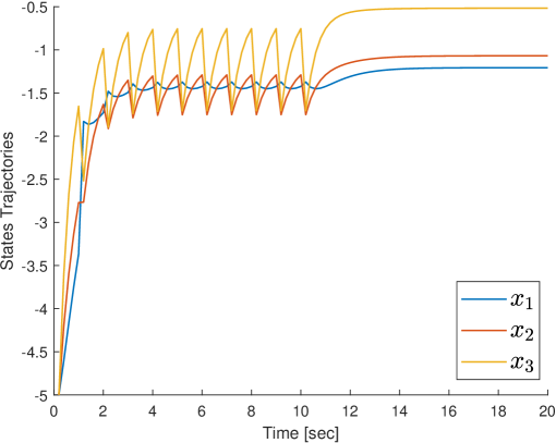
Figure 1: State trajectories under fixed point controller.

We compared computation times between monolithic and compositional abstractions for varying subsystem numbers (Table 1). Results show computation times in seconds for each abstraction and subsystem count, at a discretization parameter $n^{x}=2.5$. Compositional abstraction generally requires less time than monolithic, even as subsystems increase. The time difference remains significant; for instance, with five subsystems, compositional abstraction is almost six times faster. This makes it more computationally efficient, particularly when dealing with numerous subsystems.

Table 1: Abstraction Computation Time Comparison [s]

	2	3	4	5
Monolithic	$0.3107$	$1.2285$	$13.0902$	$5453.65$
Compositional	$0.2108$	$0.3147$	$2.2348$	$975.4288$
ratio	$1.4739$	$3.9037$	$5.8574$	$5.5910$

6 Conclusion

To conclude, this paper introduces a novel compositional technique for building symbolic models in interconnected impulsive systems using the concept of approximate alternating simulation function. With certain small gain-type conditions, our method compositionally establishes an overall alternating simulation function, connecting interconnection symbolic models and original impulsive subsystems. Moreover, we present a method, guided by stability and forward completeness, to create symbolic models with corresponding alternating simulation functions for impulsive subsystems.

Future work involves extending this approach to stochastic impulsive systems, integrating probabilistic distributions for characterizing flow and jump mode functions.

References

- [1] C. Cassandras and S. Lafortune, Introduction to Discrete Event Systems, ; Number 1. Springer Science & Business Media: Berlin/Heidelberg, Germany, 2009.
- [2] P. Tabuada, Verification and control of hybrid systems: a symbolic approach. Springer Science & Business Media, 2009.
- [3] R. Lal and P. Prabhakar, “Compositional construction of bounded error over-approximations of acyclic interconnected continuous dynamical systems,” in Proceedings of the 17th ACM-IEEE International Conference on Formal Methods and Models for System Design, pp. 1–5, 2019.
- [4] A. Saoud, P. Jagtap, M. Zamani, and A. Girard, “Compositional abstraction-based synthesis for cascade discrete-time control systems,” IFAC-PapersOnLine, vol. 51, no. 16, pp. 13–18, 2018.
- [5] M. Shahamat, J. Askari, A. Swikir, N. Noroozi, and M. Zamani, “Construction of continuous abstractions for discrete-time time-delay systems,” in 2020 59th IEEE Conference on Decision and Control (CDC), pp. 881–886, 2020.
- [6] A. Swikir and M. Zamani, “Compositional synthesis of finite abstractions for networks of systems: A small-gain approach,” Automatica, vol. 107, pp. 551–561, 2019.
- [7] M. Zamani and M. Arcak, “Compositional abstraction for networks of control systems: A dissipativity approach,” IEEE Transactions on Control of Network Systems, vol. 5, no. 3, pp. 1003–1015, 2017.
- [8] A. Swikir and M. Zamani, “Compositional abstractions of interconnected discrete-time switched systems,” in the 18th Eur. Control Conf., pp. 1251–1256, 2019.
- [9] A. Swikir and M. Zamani, “Compositional synthesis of symbolic models for networks of switched systems,” IEEE Control Systems Letters, vol. 3, no. 4, pp. 1056–1061, 2019.
- [10] A. Swikir, N. Noroozi, and M. Zamani, “Compositional synthesis of symbolic models for infinite networks,” IFAC-PapersOnLine, vol. 53, no. 2, pp. 1868–1873, 2020. 21st IFAC World Congress.
- [11] M. Sharifi, A. Swikir, N. Noroozi, and M. Zamani, “Compositional construction of abstractions for infinite networks of discrete-time switched systems,” Nonlinear Analysis: Hybrid Systems, vol. 44, p. 101173, 2022.
- [12] M. Sharifi, A. Swikir, N. Noroozi, and M. Zamani, “Compositional construction of abstractions for infinite networks of switched systems,” in 2020 59th IEEE Conference on Decision and Control (CDC), pp. 476–481, 2020.
- [13] S. Liu, N. Noroozi, and M. Zamani, “Symbolic models for infinite networks of control systems: A compositional approach,” Nonlinear Analysis: Hybrid Systems, vol. 43, p. 101097, 2021.
- [14] N. Noroozi, A. Swikir, F. R. Wirth, and M. Zamani, “Compositional construction of abstractions via relaxed small-gain conditions part ii: discrete case,” in 2018 European Control Conference (ECC), pp. 1–4, 2018.
- [15] A. Swikir, Compositional Synthesis of Symbolic Models for (In)Finite Networks of Cyber-Physical Systems. PhD thesis, Technische Universität München, 2020.
- [16] A. Saoud, A. Girard, and L. Fribourg, “Contract-based design of symbolic controllers for safety in distributed multiperiodic sampled-data systems,” IEEE Transactions on Automatic Control, vol. 66, no. 3, pp. 1055–1070, 2020.
- [17] A. Saoud, A. Girard, and L. Fribourg, “Assume-guarantee contracts for continuous-time systems,” Automatica, vol. 134, p. 109910, 2021.
- [18] A. Saoud, P. Jagtap, M. Zamani, and A. Girard, “Compositional abstraction-based synthesis for interconnected systems: An approximate composition approach,” IEEE Transactions on Control of Network Systems, vol. 8, no. 2, pp. 702–712, 2021.
- [19] S. Belamfedel Alaoui, P. Jagtap, A. Saoud, et al., “Compositional approximately bisimilar abstractions of interconnected systems,” arXiv preprint arXiv:2211.08655, 2022.
- [20] A. Swikir, A. Girard, and M. Zamani, “Symbolic models for a class of impulsive systems,” IEEE Control Systems Letters, vol. 5, no. 1, pp. 247–252, 2020.
- [21] G. Pola and P. Tabuada, “Symbolic models for nonlinear control systems: Alternating approximate bisimulations,” SIAM Journal on Control and Optimization, vol. 48, no. 2, pp. 719–733, 2009.
- [22] P. Tabuada, Verification and control of hybrid systems: A Symbolic approach. Springer Publishing Company, Incorporated, 1st ed., 2009.
- [23] A. Swikir, A. Girard, and M. Zamani, “From dissipativity theory to compositional synthesis of symbolic models,” in the 4th Indian Control Conf., pp. 30–35, 2018.