Spiralling branes and $R$-matrices

Abstract

We extend the dictionary between Type IIB branes and representations of the Ding-Iohara-Miki (DIM) algebra to the case when one of the space directions is a circle. It is well-known that the worldvolume theory on branes wrapping the circle is a $5d$ $\mathcal{N}=1$ gauge theory with adjoint matter, or more generally of cyclic quiver type, and the corresponding intertwiners of the DIM algebra give their Nekrasov partition functions. However, we find that there exists a much wider natural class of intertwiners corresponding to branes spiralling around the compactified direction, with many interesting properties. We consider two examples, one corresponding to a spiralling D5 brane and another to a D3 brane. The former gives rise to the $K$-theoretic vertex function counting sheaves on $\mathbb{C}^{3}$ while the latter produces the ‘‘non-stationary elliptic Ruijsenaars wavefunctions’’ introduced recently by Shiraishi.

To T.

1 Introduction

String theory branes can be understood on several levels. Historically they were first introduced as boundary conditions for open strings in which case they can be thought of as submanifolds of the ambient (or bulk) space, e.g. $\mathbb{R}^{10}$. However, this plain geometric description becomes inadequate if a stack of $N>1$ branes spanning the same submanifold is considered. Then, somewhat akin to Heisenberg’s development of quantum mechanics from the classical picture, the coordinates normal to the branes become matrices acting in an $N$-dimensional vector space (the Chan-Paton space) [1]. Reformulated more mathematically, a stack of branes becomes a rank $N$ vector bundle on a submanifold of the bulk space. Naturally, the bundle may be topologically nontrivial and thus some stacks of branes wrapping the same submanifold may be nonequivalent.

More generally, one would like to consider the possibility of antibranes, i.e. the objects which upon being added to the system ‘‘cancel’’ (annihilate) branes of a given type. Since there are nonequivalent stacks of branes that may live on the same submanifolds one can ask what happens if one tries to annihilate a pair of such inequivalent stacks. The result turns out to be a stack of branes on a sub-submanifold, in general of a smaller dimension. The mathematical formalism to consider branes of different dimension on equal footing is provided by coherent sheaves on the bulk space [2]. Vector bundles on submanifolds of the bulk space are examples of coherent sheaves, however the sheaf approach is more general. The essence of it is to understand vector bundles as modules over the ring of functions on the bulk space. Indeed, if $v(x)$ is a (local) section of a bundle $\mathcal{E}$ then $f(x)v(x)$ is too for every function $f(x)$ on the bulk space. Adding non-interacting branes to the system corresponds to taking the direct sum of sheaves while the annihilation is captured by introducing equivalence relation which allows one to consider complexes of sheaves.

The overall picture with modules over a ring, sums and complexes thereof begs for a representation theoretic description. It does arise on a more refined level when one considers bound states of branes. The representation space is interpreted as the Hilbert space of (BPS) bound states of a ‘‘heavy’’ brane with a number of ‘‘light’’ branes. The algebras rising in this way are called the BPS algebras [3]. Pairs of ‘‘heavy’’ branes correspond to tensor products of representations.

The BPS algebras arise in different string theories and in different backgrounds. Here we will be interested in a particular case [4] in which branes are of Type IIB string theory and the algebra is the Ding-Iohara-Miki (DIM) algebra [5]. In this approach 3- and 5-branes correspond to two different types of DIM algebra representations, collections of non-interacting branes are tensor products of representations and brane junctions are intertwining operators between ingoing and outgoing collections of branes. Also, brane crossings (when one brane passes behind another without merging) correspond to DIM $R$-matrices taken in the appropriate representations. The details about the DIM algebra, its representations and some of the intertwining operators can be found e.g. in the Appendices to [4], [12] and [23].

To make the correspondence more precise in the table below we list the main types of branes and representations we are going to consider.

$$\begin{array}[]{l|l|ccc|cc|c|c}&&&&&\lx@intercol\hfil\text{picture}\hfil\lx@intercol\vrule\lx@intercol&\tau&\\ \text{Brane}&\text{DIM rep}&{\color[rgb]{0,0,1}\mathbb{C}_{q}}&{\color[rgb]{1,0,0}\mathbb{C}_{t^{-1}}}&{\color[rgb]{.5,0,.5}\mathbb{C}_{t/q}}&\mathbb{R}_{x}&S^{1}_{y}&\mathbb{R}_{\tau}&S^{1}_{10}\\ \hline\cr{\color[rgb]{.5,0,.5}\mathrm{D5}_{q,t^{-1}}}&{\color[rgb]{.5,0,.5}\mathcal{F}^{(0,1)}_{q,t^{-1}}}&--&--&&&-&&-\\ {\color[rgb]{1,0,0}\mathrm{D5}_{q,t/q}}&{\color[rgb]{1,0,0}\mathcal{F}^{(0,1)}_{q,t/q}}&--&&--&&-&&-\\ {\color[rgb]{0,0,1}\mathrm{D5}_{t^{-1},t/q}}&{\color[rgb]{0,0,1}\mathcal{F}^{(0,1)}_{t^{-1},t/q}}&&--&--&&-&&-\\ \hline\cr{\color[rgb]{.5,0,.5}\mathrm{NS5}_{q,t^{-1}}}&{\color[rgb]{.5,0,.5}\mathcal{F}^{(1,0)}_{q,t^{-1}}}&--&--&&-&&&-\\ {\color[rgb]{1,0,0}\mathrm{NS5}_{q,t/q}}&{\color[rgb]{1,0,0}\mathcal{F}^{(1,0)}_{q,t/q}}&--&&--&-&&&-\\ {\color[rgb]{0,0,1}\mathrm{NS5}_{t^{-1},t/q}}&{\color[rgb]{0,0,1}\mathcal{F}^{(1,0)}_{t^{-1},t/q}}&&--&--&-&&&-\\ \hline\cr{\color[rgb]{.5,0,.5}\mathrm{D3}_{t/q}}&{\color[rgb]{.5,0,.5}\mathcal{V}_{t/q}}&&&--&&&-&-\\ {\color[rgb]{1,0,0}\mathrm{D3}_{t^{-1}}}&{\color[rgb]{1,0,0}\mathcal{V}_{t^{-1}}}&&--&&&&-&-\\ {\color[rgb]{0,0,1}\mathrm{D3}_{q}}&{\color[rgb]{0,0,1}\mathcal{V}_{q}}&--&&&&&-&-\\ \end{array}$$ (1)

In the setup above we consider branes on $\mathbb{C}^{3}\times\mathbb{R}^{2}\times S^{1}\times S^{1}$ and we have turned on the $\Omega$-background along the three $\mathbb{C}$ planes, its parameters being $q$, $t^{-1}$ and $t/q$ respectively. The ‘‘picture’’ label indicates what directions we are going to draw in all of the figures that follow. In our previous studies [4, 6, 11, 12] the ‘‘picture’’ directions have been a plane $\mathbb{R}_{x}\times\mathbb{R}_{y}$, but in the present short note it is essential that it is a cylinder $\mathbb{R}_{x}\tilde{\times}S^{1}_{y}$ with $S^{1}_{y}$ of radius $|\ln\Lambda|$. The tilde is meant to indicate that the cylinder has a nontrivial monodromy (is ‘‘twisted’’), i.e. when $y$ goes to $\Lambda y$ the coordinate $x$ goes to $\mu x$ (we use multiplicative notation, i.e. all the pictures are drawn in $(|\ln x|,|\ln y|)$ coordinates).

The 5-branes of Type IIB string theory are labelled by $(p,q)$-charges with $(0,1)$ being the D5 brane and $(1,0)$ the NS5 brane. General $(p,q)$-charges can be thought of as arising from bound states of several D5 and NS5 branes. The directions of the branes in the ‘‘picture’’ cylinder are dictated by their $(p,q)$-charges due to supersymmetry. 5-branes span two out of three $\mathbb{C}$-planes along which the equivariant action ($\Omega$-background) is turned on. Hence, for every $(p,q)$ charge there are three types of 5-branes: spanning $\mathbb{C}_{q}\times\mathbb{C}_{t^{-1}}$, $\mathbb{C}_{q}\times\mathbb{C}_{t/q}$ and $\mathbb{C}_{t^{-1}}\times\mathbb{C}_{t/q}$. These are labelled by the lower indices and also by color: violet, red and blue respectively. The representations corresponding to 5-branes are Fock representations e.g. $\mathcal{F}^{(1,0)}_{q,t^{-1}}(u)$ [10], i.e. spaces generated by the action of commuting creation operators $a_{-n}$ ($n\in\mathbb{N}$) from the vacuum state $|\varnothing,u\rangle$. The spectral parameter $u\in\mathbb{C}^{\times}$ of the representation indicates the position of the 5-brane on the picture cylinder. The upper indices of $\mathcal{F}$ represent $(p,q)$-charge of the brane while the lower ones indicate the pair of $\mathbb{C}$-planes it spans. 5-branes of the same color sitting at the same value of $\tau$ (the coordinate along $\mathbb{R}_{\tau}$) can have a triple junction, while the corresponding Fock representations can be joined using an intertwining operator (the analogue of an invariant tensor for the DIM algebra). This leads to the refined topological vertex [9] and $(p,q)$-brane webs [10].

D3 branes span a single $\mathbb{C}$-plane and therefore are labelled by a single index and the corresponding color $q$ (blue), $t^{-1}$ (red) or $t/q$ (violet). Classically a D3 brane spans $\mathbb{R}_{\tau}$ and lives at a point in the picture cylinder. However, with equivariant deformation turned on the coordinates of the D3 brane in the picture space become non-commutative. Hence, it does not have a well-defined position $(x,y)\in\mathbb{R}_{x}\times S^{1}_{y}$ but instead a wavefunction depending either on $x$ or on $y$ or some combination thereof. In the current short note we are going to write everything in the basis of D3 brane wavefunctions with definite $x$ coordinate and draw the D3 branes as vertical dashed lines at fixed values of $x$. D3 branes do not have $(p,q)$-charges and therefore do not change the direction of 5-branes upon joining them. The corresponding DIM representations are called vector representations $\mathcal{V}$ and they can be thought of as representations on the space of functions of $x$. We denote the basis states of the representation $\mathcal{V}$ by $|w\rangle=\delta\left(\frac{x}{w}\right)$. In fact the only states appearing in $\mathcal{V}_{q}$ are of the form $|q^{n}w\rangle$ with $n\in\mathbb{Z}$.

Branes can join together or pass behind each other in the plane of the picture. Correspondingly DIM algebra representations can be glued using an intertwiner or can be exchanged using an $R$-matrix. Many of these possibilities were explored in [4, 6, 10, 11, 12]. In the present short note we clarify how the dictionary between branes and representations works when the picture space becomes a cylinder. All local objects like brane junctions and crossings remain the same but the global structure is different which, as we will see, leads to interesting effects and novel expressions for the intertwiners.

Since the picture space is a cylinder, the branes can wrap around it. Here we need to be careful because of the twist of the cylinder. For example in general it is not possible to wrap an isolated D5 brane around $S^{1}_{y}$ since its $x$ coordinate will change to $\mu x$ after passing around the circle. If $\mu$ is nontrivial one needs extra branes with which the D5 would interact in order to glue the two ends of it. An example of such a picture is given below. Wavy lines henceforth indicate the identification of the branes passing through them — notice that pairs of corresponding wavy lines are shifted with respect to each other.

(2)

In Eq. (2) the ends of the two D5 branes are shifted because of the interaction with an NS5 brane. The gauge theory engineered by this setup is the $5d$ $\mathcal{N}=1$ $U(2)$ theory with an extra adjoint field.

In DIM representation theory compactification of the $y$ direction is normally interpreted as taking the trace over the representations corresponding to branes wrapping the circle. For example, in Eq. (2) one needs to take a trace over $\mathcal{F}^{(0,1)}_{q,t^{-1}}(w_{1})\otimes\mathcal{F}^{(0,1)}_{q,t^{-1}}(w_{2})$. The twist $\mu$ and the radius of the (complexified exponentiated) circumference of the circle $\Lambda$ are incorporated as the fugacities corresponding to the two gradings $d$ and $d_{\perp}$ on the DIM algebra (again we invite the reader to consult the Appendices of [4] and [11] for notations), so that the relevant intertwiner has the form

$$\mathop{\mathrm{Tr}}\nolimits_{\mathcal{F}^{(0,1)}_{q,t^{-1}}(w_{1})\otimes\mathcal{F}^{(0,1)}_{q,t^{-1}}(w_{2})}\Lambda^{d}\mu^{d_{\perp}}\left(\ldots\right),$$ (3)

where $(\ldots)$ denote the interactions with the NS5 brane.

The crucial observation is that there are more general brane configurations on the cylinder satisfying the conditions of supersymmetry and corresponding to interesting operators in DIM representation theory. Those appear when a vertical brane goes full circle around $S^{1}_{y}$ but does not return to the same $x$ position. Then the brane can continue to the next circle and so on, possibly for an infinite number of wrappings. We call such configurations spiralling branes. Algebraically these are not traces of the combinations of intertwiners ‘‘along the compactification direction’’, at least not traces of any finite number of them. Nevertheless the resulting expressions are covariant with respect to DIM transformations, and this fact ensures their nice properties.

In this short letter we provide two examples of configurations involving spiralling branes.

1. The first setup is a D5_q,t/q brane spiralling around $S^{1}_{y}$ crossing an NS5${}_{q,t^{-1}}$ brane (see Fig. 1). We will find that the matrix element of the intertwining operator corresponding to Fig. 1 is given by the $K$-theoretic vertex function [13, 14] counting sheaves on $\mathbb{C}^{3}$.

2. The second setup is a stack of $N$ D3_q brane spiralling and eventually joining a stack of $N$ NS5${}_{q,t^{-1}}$ branes as shown in Fig. 2. The resulting operator turns out to reproduce the screened vertex operator introduced by Shiraishi in [15, 16] (see also [18]). Let us note that for specific choice of deformation parameters the screened vertex operator has been obtained in [17]. This choice corresponds to the case when the D3 brane spiral becomes tighter and tighter essentially collapsing into a circle (the situation is slightly more complicated, as we discuss in sec. 5, but the main idea is true).

These two examples are meant to demonstrate the usefulness of the novel concept of spiralling branes. It is already clear that many more applications can be explored. Also the physical meaning of the spiralling does not seem to be completely understood; this will be explored elsewhere.

The rest of the paper is organized as follows. In sec. 2 we remind some of the results of [12], in sec. 3 we compute the matrix elements of the setup from Fig. 1 and show that it coincides with the $K$-theoretic vertex function. In sec. 4 we use the $R$-matrices in the tensor product of Fock and vector representation to construct the screened vertex operator which reproduces that of Shiraishi. We list some of the ideas for the future in sec. 6.

Figure 1: The configuration with spiralling D5_q,t/q brane crossing NS5${}_{q,t^{-1}}$ brane. Every turn of the spiral is shifted by $\mu$ while the circumference of the circle is $\Lambda$. Pairs of wavy or slanted lines indicate identification of the branes sticking into them. Notice that the crossings to the left of the center are over, while those to the right are under. The Young diagrams $\lambda^{(i)}$ are interlacing as in Eq. (17).

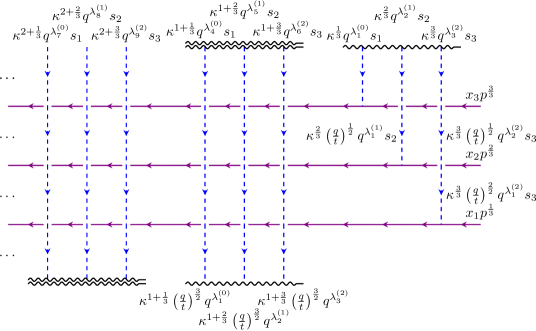
Figure 2: The configuration of $N$ spiralling D3_q branes and $N$ horizontal NS5${}_{q,t^{-1}}$ branes ($N=3$ in the picture). In order not to clutter the figure not all spectral parameters of the branes are shown.

2 Reminder: Hanany-Witten 5-brane crossing operators

Let us remind the main result of [12] (we use the same notation throughout the paper). It turns out that the $R$-matrix acting in the tensor product $\mathcal{F}^{(0,1)}_{q,t/q}(w)\otimes\mathcal{F}^{(1,0)}_{q,t^{-1}}(u)$ is exactly computable and has interesting combinatorial properties. We call the resulting operator the Hanany-Witten (HW) brane crossing operator. The $(\lambda,\mu)$ matrix element of the $R$-matrix taken along the vertical Fock representation in the standard Macdonald polynomial basis is given by:

$$\widetilde{\mathcal{R}}^{\lambda}_{\mu}(w,u)=\left(\ldots\otimes\left\langle\mu,\sqrt{\frac{t}{q}}w\right|\right)\mathcal{R}|_{\mathcal{F}^{(0,1)}_{q,t/q}(w)\otimes\mathcal{F}^{(1,0)}_{q,t^{-1}}(u)}\left(|\lambda,w\rangle\otimes\ldots\right)=\\ =\quad\includegraphics[valign={c}]{figures/d5-ns5-hw-lm-crop}=\\ =\quad u^{|\lambda|-|\mu|}f^{\lambda}_{\mu}t^{\frac{\hat{Q}}{2}}\exp\left[-\sum_{n\geq 1}\frac{1-t^{-n}}{n}\left[\frac{1}{1-q^{n}}+\left(\frac{t}{q}\right)^{n}\mathrm{Ch}_{\mu}\left(q^{n},\left(t/q\right)^{n}\right)-\mathrm{Ch}_{\lambda}\left(q^{n},\left(t/q\right)^{n}\right)\right]w^{n}a_{-n}\right]\times\\ \times\exp\left[\sum_{n\geq 1}\frac{1-t^{n}}{n}\left[\mathrm{Ch}_{\mu}\left(q^{-n},\left(t/q\right)^{-n}\right)-\mathrm{Ch}_{\lambda}\left(q^{-n},\left(t/q\right)^{-n}\right)\right]w^{-n}a_{n}\right],$$ (4)

where

$$\mathrm{Ch}_{\lambda}(q_{1},q_{2})=\sum_{(i,j)\in\lambda}q_{1}^{j-1}q_{2}^{i-1},$$ (5)

the generators $a_{n}$ acting on the horizontal Fock space $\mathcal{F}^{(1,0)}_{q,t^{-1}}(u)$ satisfy

$$[a_{n},a_{m}]=\frac{1-q^{|n|}}{1-t^{|n|}}n\delta_{n+m,0},$$ (6)

and the prefactor $f^{\lambda}_{\mu}$ is nonvanishing only when the partitions $\lambda$ and $\mu$ are interlacing:

$$f^{\lambda}_{\mu}=0\quad\text{for }\lambda\nsucc\mu$$ (7)

which means

$$\lambda\succ\mu\qquad\Leftrightarrow\qquad\ldots\geq\lambda_{i}\geq\mu_{i}\geq\lambda_{i+1}\geq\mu_{i+1}\geq\ldots$$ (8)

The operator $t^{\hat{Q}/2}$ shifts the spectral parameter $u$ of the horizontal Fock space by $\sqrt{t}$:

$$t^{\hat{Q}/2}|u,\alpha\rangle=|\sqrt{t}u,\alpha\rangle.$$ (9)

The interlacing condition (8) endows the $R$-matrix (4) with nice combinatorial properties. We will use them when we combine several brane crossing operators together in a chain.

In addition to the formula (4) which can be called the undercrossing (as evident from the picture) we can derive the formula for overcrossing, i.e. when the branes pass each other in different order in the $\tau$ coordinate. This corresponds to evaluating the inverse of the $R$-matrix. We find

$$(\widetilde{\mathcal{R}}^{-1})^{\lambda}_{\mu}(w,u)=\left(\ldots\otimes\left\langle\mu,\sqrt{\frac{q}{t}}w\right|\right)\mathcal{R}^{-1}|_{\mathcal{F}^{(0,1)}_{q,t/q}(w)\otimes\mathcal{F}^{(1,0)}_{q,t^{-1}}(u)}\left(|\lambda,w\rangle\otimes\ldots\right)=\\ =\quad\includegraphics[valign={c}]{figures/d5-ns5-hw-lm-over-crop}=\\ =\quad u^{|\lambda|-|\mu|}g^{\lambda}_{\mu}t^{-\frac{\hat{Q}}{2}}\exp\left[-\sum_{n\geq 1}\frac{1-t^{-n}}{n}\left[\mathrm{Ch}_{\mu}\left(q^{n},\left(t/q\right)^{n}\right)-\mathrm{Ch}_{\lambda}\left(q^{n},\left(t/q\right)^{n}\right)\right]w^{n}a_{-n}\right]\times\\ \times\exp\left[\sum_{n\geq 1}\frac{1-t^{n}}{n}\left(\frac{t}{q}\right)^{n}\left[-\frac{1}{1-q^{-n}}+\mathrm{Ch}_{\mu}\left(q^{-n},\left(t/q\right)^{-n}\right)-\left(\frac{q}{t}\right)^{n}\mathrm{Ch}_{\lambda}\left(q^{-n},\left(t/q\right)^{-n}\right)\right]w^{-n}a_{n}\right],$$ (10)

where the prefactor $g^{\lambda}_{\mu}$ now requires $\mu$ to interlace $\lambda$, not vice versa:

$$g^{\lambda}_{\mu}=0\quad\text{for }\mu\nsucc\lambda.$$ (11)

Notice that the expression (10) is a generalization of Eq. (67) from [11] to which it reduces for $\lambda=\mu=\varnothing$.

One can also write down the Hanany-Witten (HW) move [19] relating the over- and undercrossing operators (4) and (10). The key combinatorial observation is that if $\lambda\succ\mu$, then $\mu\succ[\lambda\backslash\lambda_{1}]$, where $[\lambda\backslash\lambda_{1}]$ denotes the Young diagram obtained from $\lambda$ by removing the first column. We then have

$$(\widetilde{\mathcal{R}})^{\lambda}_{\mu}(w,u)\sim\Phi^{q}_{q,t^{-1}}(q^{\lambda_{1}}w)(\widetilde{\mathcal{R}}^{-1})^{[\lambda\backslash\lambda_{1}]}_{\mu}\left(\frac{t}{q}w,u\right),$$ (12)

where $\Phi^{q}_{q,t^{-1}}(w)$ is the D3_q-NS5${}_{q,t^{-1}}$ brane junction operator [4]:

$$\Phi^{q}_{q,t^{-1}}(q^{\lambda_{1}}w)\sim u^{\lambda_{1}}t^{\hat{Q}}:\exp\left[\sum_{n\neq 0}\frac{1-t^{n}}{n}\frac{q^{-n\lambda_{1}}}{1-q^{-n}}a_{n}w^{-n}\right]:.$$ (13)

Graphically one can picture the HW move as follows:

$$\includegraphics[valign={c}]{figures/d5-ns5-hw-lm-crop}\quad=\quad\includegraphics[valign={c}]{figures/hw-creation-crop}$$ (14)

The junction between the dashed blue line and the vertical red line is a trivial operator cutting the Young diagram $\lambda$ into the first column $\lambda_{1}$ and the rest of the diagram $[\lambda\backslash\lambda_{1}]$.

As a side remark let us notice a curious fact that the Hanany-Witten rule [19] also holds for the crossing and junction operators that we have introduced. The rule states that between a given pair of D5_q,t/q and NS5${}_{q,t^{-1}}$ branes there can stretch at most one D3_q brane. Indeed, one can evaluate the operator corresponding to the following picture

$$\includegraphics[valign={c}]{figures/hw-creation-3-crop}\quad\sim\quad\frac{\left(q^{\lambda_{2}-\lambda_{1}};q\right)_{\infty}}{\left(tq^{\lambda_{2}-\lambda_{1}};q\right)_{\infty}}$$ (15)

and learn that it vanishes since $\lambda_{1}\geq\lambda_{2}$ in a Young diagram.

3 Spiralling 5-branes and the $K$-theoretic vertex

As noted in [12] the interlacing conditions (7), (11) for the Young diagrams on the legs of the HW crossings (4), (10) remind one of diagonal slices of a $3d$ Young diagram (plane partitions). Indeed, if $\pi=\{\pi^{(i)}_{j}\}$, $i,j\in\mathbb{N}$ is a plane partition, so that $\pi^{(i)}_{j}\geq\pi^{(i+1)}_{j}$, $\pi^{(i)}_{j}\geq\pi^{(i)}_{j+1}$, then the set of Young diagrams $\{\lambda^{(i)}\}$ defined by

$$\lambda^{(i)}_{j}=\pi^{(j)}_{i+j-1},\quad i\in\mathbb{Z},j\in\mathbb{N}.$$ (16)

satisfies the interlacing conditions

$$\ldots\prec\lambda^{(-3)}\prec\lambda^{(-2)}\prec\lambda^{(-1)}\prec\lambda^{(0)}\succ\lambda^{(1)}\succ\lambda^{(2)}\succ\lambda^{(3)}\succ\ldots$$ (17)

Notice that the infinite tails in the sequence (17) may have nontrivial asymptotics.

This makes one wonder if the sequence of Young diagrams (17) can be understood as living on the legs of a chain of HW crossing operators. It is not hard to guess the right configuration of branes, which turns out to be a spiralling D5_q,t/q brane crossing a horizontal NS5${}_{q,t^{-1}}$ brane, as shown in Fig. 1. The Figure depicts an intertwining of the DIM algebra involving an infinite chain of $R$-matrices in which the sum over intermediate states on the vertical Fock representation corresponds to the sum over plane partitions. Let us emphasize this is not the sum over plane partitions featuring in the (refined) topological vertex/triple 5-brane junction, each slice here originates from its own segment of the D5_q,t/q brane and it is essential that the number of segments (and crossings) is infinite.

The algebraic expression for the intertwiner in Fig. 1 is

$$\mathfrak{R}=\left[\prod_{i=-\infty}^{-1}(\Lambda^{id}\mu^{id^{\perp}}\otimes 1)\mathcal{R}^{-1}(\Lambda^{(1-i)d}\mu^{(1-i)d^{\perp}}\otimes 1)\right]\mathcal{R}\times\\ \times\left.\left[\prod_{i=1}^{\infty}(\Lambda^{id}\mu^{id^{\perp}}\otimes 1)\mathcal{R}(\Lambda^{(1-i)d}\mu^{(1-i)d^{\perp}}\otimes 1)\right]\right|_{\mathcal{F}^{(0,1)}_{q,t/q}\otimes\mathcal{F}^{(1,0)}_{q,t^{-1}}}.$$ (18)

In fact $\mathfrak{R}$ is a Drinfeld twist of the standard DIM $R$-matrix using the cocycle $F=\left[\prod_{i=1}^{\infty}(\Lambda^{d}\mu^{d^{\perp}}\otimes 1)\mathcal{R}\right]$. Since $\mathfrak{R}$ acts on the tensor product of two Fock spaces its matrix elements depend on four Young diagrams — the asymptotics of the sequences of states on the vertical and horizontal branes.

The next logical question is what natural object can be associated with the sum over plane partitions? A very interesting candidate is the $K$-theoretic vertex, the equivariant count of sheaves on $\mathbb{C}^{3}$ [13, 14]. The vertex is given by an explicit formula:

$$I(\lambda,\mu,\nu)=\sum_{\pi}Q^{|\pi|^{\prime}}\exp\left[\sum_{n\geq 1}\frac{1}{n}\chi_{\pi}(t_{1}^{n},t_{2}^{n},t_{3}^{n})\right],$$ (19)

where the sum goes over plane partitions with fixed asymptotics $(\lambda,\mu,\nu)$ along three coordinate axes, $|\pi|^{\prime}$ denotes the regularized total number of boxes in $\pi$,

$$\chi_{\pi}(t_{1},t_{2},t_{3})=\mathrm{Ch}_{\pi}(t_{1},t_{2},t_{3})-\frac{\mathrm{Ch}_{\pi}(t_{1}^{-1},t_{2}^{-1},t_{3}^{-1})}{t_{1}t_{2}t_{3}}+\mathrm{Ch}_{\pi}(t_{1},t_{2},t_{3})\mathrm{Ch}_{\pi}(t_{1}^{-1},t_{2}^{-1},t_{3}^{-1})\frac{(1-t_{1})(1-t_{3})(1-t_{3})}{t_{1}t_{2}t_{3}}$$ (20)

and

$$\mathrm{Ch}_{\pi}(t_{1},t_{2},t_{3})=\sum_{(i,j,k)\in\pi}t_{1}^{j-1}t_{2}^{i-1}t_{3}^{k-1}.$$ (21)

We find quite remarkable that the following theorem holds.

Theorem 1.

Up to $\Lambda$- and $\mu$-independent prefactors the $K$-theoretic vertex with two nontrivial asymptotics coincides with the vacuum matrix element of $\mathfrak{R}$

$$(\langle\varnothing|\otimes\langle\mu|)\mathfrak{R}(|\lambda\rangle\otimes|\varnothing\rangle)\sim I(\lambda,\mu,\varnothing)$$ (22)

provided one identifies

$$t_{1} =\mu^{-1}\sqrt{\frac{t}{q}},$$ (23)

$$t_{2} =\mu\sqrt{\frac{t}{q}},$$ (24)

$$t_{3} =q,$$ (25)

$$Q =\Lambda.$$ (26)

The proof is straightforward term-by-term analysis of the matrix elements of $\mathfrak{R}$. Several remarks are in order.

1. Notice that $t_{1}t_{2}t_{3}=t$, so one can nicely write three independent parameters $(t_{1},_{2},t_{3})$ in terms of four parameters $(t_{1},t_{2},t_{3},(t_{1}t_{2}t_{3})^{-1})=\left(\mu^{-1}\sqrt{\frac{t}{q}},\mu\sqrt{\frac{t}{q}},q,t^{-1}\right)$ with product equal to one.

2. In the definition of $\mathfrak{R}$ the built-in symmetry of the DIM algebra under permutations of $(q,t^{-1},t/q)$ is broken. Instead the new symmetry between $(t_{1},t_{2},t_{3})$ emerges in a completely nontrivial way.

3. It is not hard to add the third nontrivial leg to the vertex by considering instead of $\mathfrak{R}$, i.e. a product of the form $\cdots\mathcal{R}^{-1}\mathcal{R}^{-1}\mathcal{R}^{-1}\mathcal{R}\mathcal{R}\mathcal{R}\cdots$, a more general product of $\pm 1$ powers with the same asymptotics. Such a pattern of $\pm 1$ powers encodes a Maya diagram which is equivalent to a Young diagram, which is the diagram living on the third leg in the $K$-theoretic vertex.

4. The infinite wrapping of the D5_q,t/q brane and the appearance of $\mu$ as an extra equivariant parameter in the vertex suggest that the extra sums over an infinite number of Young diagrams could be rewritten as sums over Kaluza-Klein modes in the $S^{1}_{y}$ direction. It would be interesting to make this point more explicit in the future.

5. Non-vacuum matrix elements of $\mathfrak{R}$ should give $K$-theoretic vertex with descendant insertions.

4 Shiraishi wavefunctions from spiralling D3-branes

In [15, 16] Shiraishi has introduced a new class of special functions originally called ‘‘non-stationary elliptic Ruijsenaars wavefunctions’’. We will call them simply Shiraishi functions for brevity. These functions can be obtained as matrix elements of a certain screened vertex operator involving affine system of screening currents. In this section we show that the affine screening operators featuring in the Shiraishi vertex operator naturally arise in the wrapped background with spiralling D3_q branes.

Consider a tensor product of $N$ horizontal Fock spaces $\mathcal{F}^{(1,0)}_{q,t^{-1}}\left(p^{\frac{i}{N}}x_{i}\right)$. Then according to the general formalism [4] there are screening currents between neighbouring pairs of Fock spaces built from intertwiners of DIM algebra involving vector representations $\mathcal{V}_{q}$ or $\mathcal{V}_{t^{-1}}$ (these are usually called dual sets of screening charges). However, the essential difference from [4] arises because the space is now compactified, so there appears an extra screening charge corresponding to the interaction between the first and the last Fock spaces in the tensor product.

The Shiraishi wavefunction $f^{\widehat{\mathfrak{gl}}_{N}}$ depends on two sets of $N$ variables $\mathbf{x}=\{x_{i}\}$ and $\mathbf{s}=\{s_{i}\}$ and parameters $p$, $\kappa$, $q$ and $t$. It can be defined as a vacuum matrix element of a vertex operator as follows:

$$f^{\widehat{\mathfrak{gl}}_{N}}(\mathbf{x},p^{\frac{1}{N}}|\mathbf{s},\kappa^{\frac{1}{N}}|q,t)=\prod_{1\leq i<j\leq N}\frac{\left(\kappa^{\frac{j-i}{N}}t\frac{s_{j}}{s_{i}};q,\kappa\right)_{\infty}\left(\kappa^{\frac{j-i}{N}}\frac{q}{t}\frac{s_{j}}{s_{i}};q,\kappa\right)_{\infty}}{\left(\kappa^{\frac{j-i}{N}}\frac{s_{j}}{s_{i}};q,\kappa\right)_{\infty}\left(\kappa^{\frac{j-i}{N}}q\frac{s_{j}}{s_{i}};q,\kappa\right)_{\infty}}\langle\varnothing|\prod_{i=0}^{N-1}\Phi^{i}(s_{i+1}|t^{\omega^{N-i}}\mathbf{x},p)|\varnothing\rangle,$$ (27)

where

$$(x;q,p)_{\infty} =\prod_{i,j\geq 0}(1-xq^{i}p^{j}),$$ (28)

$$t^{\omega^{m}}\mathbf{x} =(x_{1},x_{2},\ldots,tx_{N-i+1},\ldots,tx_{N})$$ (29)

$$\Phi^{i}(s|t^{\omega^{N-i}}\mathbf{x},p) =\sum_{\lambda}\Phi_{\lambda}^{i}(s)\left(p^{\frac{1}{N}}\prod_{j\geq 1}\frac{t^{\delta_{j\mod N,1}}x_{(N-i+j)\mod N}}{x_{(N-i+j-1)\mod N}}\right)^{\lambda_{j}},$$ (30)

$$\Phi^{i}_{\lambda}(s) =\left(\frac{\left(\frac{q}{t};q\right)_{\infty}}{\left(q;q\right)_{\infty}}\right)^{l(\lambda)}\phi_{i-l(\lambda)}(s)\prod_{j=1}^{l(\lambda)}S_{j-i+1}\left(\kappa^{\frac{l(\lambda)}{N}}q^{\lambda_{j}}s\right),$$ (31)

$$\phi_{i}(s) =:\exp\left[\sum_{n\neq 0}\frac{w^{-n}}{n}\beta_{n}^{(i)}\right]:,$$ (32)

$$S_{i}(w) =:\exp\left[-\sum_{n\neq 0}\frac{w^{-n}}{n}\alpha^{(i)}_{n}\right]:,$$ (33)

and the bosonic modes $\alpha^{(i)}_{n}$, $\beta^{(i)}_{n}$ satisfy certain Heisenberg commutation relations based on the affine root system. The exact expressions for these commutation relations can be found in [15].

The main theorem in this section states that one can reproduce all the screening currents and vertex operators in (32) and (33) if one considers the system of spiralling branes depicted in Fig. 2.

Theorem 2.

The vacuum matrix element in the r.h.s. of (27) coincides with the vacuum matrix element of the intertwiner shown in Fig. 2. The map between the parameters is already incorporated in the Figure.

The proof is tedious but straightforward and involves checking the commutation relations of the screening currents and establishing the map between the parameters of the Shiraishi functions and the spectral parameters of the representations in the DIM intertwiner. In fact, more can be said: not only does the vacuum matrix elements coincide, but the screened vertex operator itself is the same as the intertwiner from Fig. 2.

Notice that Theorem 2 provides the identification between the network of DIM intertwiners and the wavefunction for completely general parameters. One can then follow the dictionary between the parameters for any possible degeneration, such as the one considered in [17].

Having new algebraic view on Shiraishi functions gives us hints about their properties. In the next section we provide as just one example, the sketch of a proof of the mirror symmetry of the functions $f^{\widehat{\mathfrak{gl}}_{N}}$.

5 Symmetries of Shiarishi wavefunctions from spiralling branes

Functions $f^{\widehat{\mathfrak{gl}}_{N}}(\mathbf{x},p^{\frac{1}{N}}|\mathbf{s},\kappa^{\frac{1}{N}}|q,t)$ have nontrivial symmetry properties which are not evident from their definition. In partocular, they enjoy the so-called mirror symmetry (the exact prefactor is also known [15], but we will not pursue it here):

$$f^{\widehat{\mathfrak{gl}}_{N}}(\mathbf{x},p^{\frac{1}{N}}|\mathbf{s},\kappa^{\frac{1}{N}}|q,t)\sim f^{\widehat{\mathfrak{gl}}_{N}}(\mathbf{s},\kappa^{\frac{1}{N}}|\mathbf{x},p^{\frac{1}{N}}|q,q/t).$$ (34)

In the spiralling branes formalism the symmetry (34) becomes the consequence of the HW move (14). Indeed, after a little manipulation (attaching the free ends of the D3_q branes to D5_q,t/q branes, which adds only a prefactor to the partition function [11]) one learns that Fig. 2 is equivalent to the following picture:

(35)

Using the HW move (14) we can eliminate D3_q branes altogether and encode their positions in the pattern of over- and undercrossings:

(36)

It might not be evident from the first sight, but after a little redrawing one can see that the picture (36) is symmetric under the exchange of the vertical and horizontal axes and simultaneous swap of red and violet colors (i.e. $t^{-1}$ and $t/q$ parameters). This proves the mirror symmetry of Shiraishi wavefunctions.

Spectral duality of the Shiraishi wavefunctions can also be proven along the same lines, the details of this will appear elsewhere.

6 Conclusions

We have introduced new types of brane configurations in Type IIB string theory on the twisted product $\mathbb{R}^{8}\tilde{\times}T^{2}$. In these configurations a brane wraps one of the cycles of the torus multiple times while with every wrapping one of the flat coordinates is shifted by a constant. It turns out that such brane configurations are meaningful also in the algebraic formalism in which they correspond to certain DIM algebra intertwiners.

To justify the usefulness of the spiralling branes we considered two examples in which the corresponding intertwining operators reproduce beautiful objects ($K$-theoretic vertex function and Shiraishi wavefunctions) that are both of high importance to general mathematical physics.

We hope that this approach will lead to many new results, however as for now we have only scratched the surface. Nevertheless we have proven mirror symmetry of Shiraishi wavefunctions which turns out to be natural in our formalism. With the new machinery it would also be desirable to understand Hamiltonians corresponding to ‘‘nonstationary elliptic Ruijsenaars’’ system.

Let us comment on possible connection with the natural generalization of the $K$-theoretic vertex function — the ‘‘magnificent four’’ vertex function [25], which is a partition function counting $4d$ Young diagrams (solid partitions). We conjecture based on the combinatorics of the crossing operators that the setup similar to that of Fig. 1 but with a D7 brane instead of the D5 brane will in fact reproduce the magnificent four vertex. In the alebraic language this corresponds to wrapping the MacMahon representation instead of the Fock one on the spiral. One can also see that a similar crossing but with D5${}_{q,t^{-1}}$ crossing NS5${}_{q,t^{-1}}$ leads to a partition function that can be understood as a particular reduction of the magnificent four vertex in which the $4d$ Young diagrams are confined to a ‘‘hook’’ in one of the coordinate planes.

Very recently, $4d$ Young diagrams have also been considered as states of BPS particles arising from the bound states of branes [26]. It would be interesting to incorporate them into our algebraic description.

An explicit closed form expression for the $K$-theoretic vertex with two nontrivial legs was obtained in [24]. Our approach does not seem to give a reason for the existence of such an expression, however this deserves further investigation.

We also expect that spiralling branes can be used in the new algebraic approach to $qq$-characters [23] to accommodate gauge theories with adjoint matter.

References

- [1] J. Polchinski, Cambridge University Press, 2007, ISBN 978-0-511-25227-3, 978-0-521-67227-6, 978-0-521-63303-1 doi:10.1017/CBO9780511816079
- [2] E. Sharpe, [arXiv:hep-th/0307245 [hep-th]].
- [3] J. A. Harvey and G. W. Moore, Commun. Math. Phys. 197 (1998), 489-519 doi:10.1007/s002200050461 [arXiv:hep-th/9609017 [hep-th]].
- [4] Y. Zenkevich, JHEP 08 (2021), 149 doi:10.1007/JHEP08(2021)149 [arXiv:1812.11961 [hep-th]].
-
[5]
J. Ding, K.
Iohara, Lett. Math. Phys. 41 (1997) 181–193, q-alg/9608002
K. Miki, J. Math. Phys. 48 (2007) 123520 - [6] Y. Zenkevich, JHEP 12 (2021), 034 doi:10.1007/JHEP12(2021)034 [arXiv:1912.13372 [hep-th]].
-
[7]
D. Gaiotto and M. Rapčák,
JHEP 01 (2019), 160
doi:10.1007/JHEP01(2019)160
[arXiv:1703.00982 [hep-th]].
T. Procházka and M. Rapčák, JHEP 11 (2018), 109 doi:10.1007/JHEP11(2018)109 [arXiv:1711.06888 [hep-th]].
T. Procházka and M. Rapčák, JHEP 05 (2019), 159 doi:10.1007/JHEP05(2019)159 [arXiv:1808.08837 [hep-th]].
M. Rapčák, JHEP 01 (2020), 042 doi:10.1007/JHEP01(2020)042 [arXiv:1910.00031 [hep-th]]. -
[8]
D. Galakhov,
Nucl. Phys. B 946 (2019), 114693
doi:10.1016/j.nuclphysb.2019.114693
[arXiv:1812.05801 [hep-th]].
D. Galakhov and M. Yamazaki, Commun. Math. Phys. 396 (2022) no.2, 713-785 doi:10.1007/s00220-022-04490-y [arXiv:2008.07006 [hep-th]].
D. Galakhov, W. Li and M. Yamazaki, JHEP 08 (2021), 146 doi:10.1007/JHEP08(2021)146 [arXiv:2106.01230 [hep-th]]. -
[9]
H. Awata and H. Kanno,
JHEP 05 (2005), 039
doi:10.1088/1126-6708/2005/05/039
[arXiv:hep-th/0502061 [hep-th]].
A. Iqbal, C. Kozcaz and C. Vafa, JHEP 0910 (2009) 069 doi:10.1088/1126-6708/2009/10/069 [hep-th/0701156]. - [10] H. Awata, B. Feigin and J. Shiraishi, JHEP 1203 (2012) 041 doi:10.1007/JHEP03(2012)041 [arXiv:1112.6074 [hep-th]].
- [11] Y. Zenkevich, JHEP 12 (2021), 027 doi:10.1007/JHEP12(2021)027 [arXiv:2012.15563 [hep-th]].
- [12] Y. Zenkevich, [arXiv:2212.14808 [hep-th]].
- [13] N. Nekrasov and A. Okounkov, doi:10.14231/AG-2016-015 [arXiv:1404.2323 [math.AG]].
- [14] A. Okounkov, [arXiv:1512.07363 [math.AG]].
- [15] J. I. Shiraishi, Journal of Integrable Systems, 4(1) (2019): xyz010. [arXiv:1903.07495 [math.QA]]
- [16] E. Langmann, M. Noumi and J. Shiraishi, SIGMA 16 (2020), 105 doi:10.3842/SIGMA.2020.105 [arXiv:2006.07171 [math-ph]].
- [17] M. Fukuda, Y. Ohkubo and J. Shiraishi, SIGMA 16 (2020), 116 doi:10.3842/SIGMA.2020.116 [arXiv:2002.00243 [math.QA]].
-
[18]
H. Awata, H. Kanno, A. Mironov and A. Morozov,
JHEP 04 (2020), 212
doi:10.1007/JHEP04(2020)212
[arXiv:1912.12897 [hep-th]].
H. Awata, H. Kanno, A. Mironov and A. Morozov, JHEP 08 (2020), 150 doi:10.1007/JHEP08(2020)150 [arXiv:2005.10563 [hep-th]]. - [19] A. Hanany and E. Witten, Nucl. Phys. B 492 (1997), 152-190 doi:10.1016/S0550-3213(97)00157-0 [arXiv:hep-th/9611230 [hep-th]].
-
[20]
H. Awata, H. Kanno, A. Mironov, A. Morozov, A. Morozov, Y. Ohkubo and Y. Zenkevich,
JHEP 10 (2016), 047
doi:10.1007/JHEP10(2016)047
[arXiv:1608.05351 [hep-th]].
H. Awata, H. Kanno, A. Mironov, A. Morozov, A. Morozov, Y. Ohkubo and Y. Zenkevich, Nucl. Phys. B 918 (2017), 358-385 doi:10.1016/j.nuclphysb.2017.03.003 [arXiv:1611.07304 [hep-th]].
H. Awata, H. Kanno, A. Mironov, A. Morozov, K. Suetake and Y. Zenkevich, JHEP 04 (2019), 097 doi:10.1007/JHEP04(2019)097 [arXiv:1810.07676 [hep-th]]. - [21] M. Jimbo, H. Konno, S. Odake and J. Shiraishi, Transform. Groups 4 (1999), 303-327 doi:10.1007/BF01238562 [arXiv:q-alg/9712029 [math.QA]].
- [22] M. Ghoneim, C. Kozçaz, K. Kurşun and Y. Zenkevich, Nucl. Phys. B 978 (2022), 115740 doi:10.1016/j.nuclphysb.2022.115740 [arXiv:2012.15352 [hep-th]].
- [23] M. B. Bayındırlı, D. N. Demirtaş, C. Kozçaz and Y. Zenkevich, [arXiv:2310.02587 [hep-th]].
- [24] Y. Kononov, A. Okounkov and A. Osinenko, Commun. Math. Phys. 382 (2021) no.3, 1579-1599 doi:10.1007/s00220-021-03936-z [arXiv:1905.01523 [math-ph]].
-
[25]
N. Nekrasov,
Ann. Inst. H. Poincare D Comb. Phys. Interact. 7 (2020) no.4, 505-534
doi:10.4171/aihpd/93
N. Nekrasov and N. Piazzalunga, [arXiv:2306.12995 [hep-th]]. - [26] D. Galakhov and W. Li, [arXiv:2311.02751 [hep-th]].