The quantum beam splitter with many partially indistinguishable photons: multiphotonic interference and asymptotic classical correspondence

Abstract

We present the asymptotic analysis of the quantum two-port interferometer in the $n\rightarrow\infty$ limit of $n$ partially indistinguishable photons. Using the unitary-unitary duality between port and inner-mode degrees of freedom, the probability distribution of output port counts can be decomposed as a sum of contributions from independent channels, each associated to a spin-$j$ representation of $SU(2)$ and, in this context, to $2j$ effectively indistinguishable photons in the channel. Our main result is that the asymptotic output distribution is dominated by the $O(\sqrt{n})$ channels around a certain $j^{*}$ that depends on the degree of indistinguishability. The asymptotic form is essentially the doubly-humped semi-classical envelope of the distribution that would arise from $2j^{*}$ indistinguishable photons, and which reproduces the corresponding classical intensity distribution.

The concept of interference is fundamental to our understanding of light, particularly in its classical wave-like manifestations, as demonstrated by the Michelson interferometer [1]. However, with the advent of photon-pair sources, a more nuanced type of interference has become accessible, namely the quantum interference of multiphotonic probability amplitudes [2] as exemplified by the Shih-Alley-Hong-ou-Mandel (HOM) experiment [3, *shih_new_1988, *legero_time-resolved_2003, *bouchard_two-photon_2021]. The Michelson and HOM interferometers can be respectively understood as the macroscopic and microscopic limits of the standard scenario of two independent light sources interfering via a beam splitter [7][8, *luis_quantum_1995, *fearn_quantum_1987]. A natural question then arises: what is the interplay between the classical and quantum notions of interference as the number $n$ of impinging photons scales from the two-photon HOM limit to the macroscopic many-photon Michelson limit?

This connection between the granular and macroscopic behaviors of light at the beam splitter has been the subject of considerable interest [7, 11, 12, 13]. The best understood case is the extension of the HOM scenario to many perfectly indistinguishable photons; that is, identical photons in all degrees of freedom that are ancillary to the path (frequency, polarization, momentum, etc.), which henceforth will be named inner-modes. Here, the problem can be framed in the language of angular momentum [7], where the probability amplitudes are given by elements of the spin-$j$ representation matrix of the $SU(2)$ beam splitter transformation. In the large $n$ limit, a coexistence of classical and quantum interference effects [7, 11] is found: the probability distribution of output port counts shows rapid oscillations due to multiphotonic interference, modulated by an envelope corresponding to the classical distribution of output intensities from two interfering beams with a random relative phase.

The case of the HOM setting with many partially indistinguishable photons is less understood. One approach is that of references [12, *tichy_interference_2014, *tichy_extending_2017] where the resulting statistics are decomposed in terms of “distinguishability types” labeled by the conserved occupation numbers in an orthogonal inner mode basis. More recent approaches to dealing with the problem of partial indistinguishability in multiphoton interference have emphasized a decomposition based on the so-called unitary-unitary duality, where another good quantum number emerges labelling $SU(N)$ irreducible representations [15, 16, 17]. In the two-port ($N=2$) case, this number corresponds to a spin-$j$ common to path and inner mode degrees of freedom. Although these approaches can be extended to large numbers of photons, the asymptotic analysis of the output distribution in the HOM setting with partially indistinguishable photons has not been presented yet.

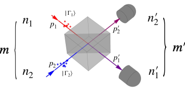
Figure 1: Schematic of the quantum two-port interferometer with partially indistinguishable photons. $m$ and $m^{\prime}$ measure the input and output port imbalance respectively.

In this work we present this asymptotic analysis of the HOM multiphoton interferometer with partially indistinguishable photons using the decomposition based on unitary-unitary duality between port and inner-modes degrees of freedom. This decomposition makes evident how entanglement between the two degrees of freedom is the decoherence mechanism underlying the loss of visibility of multiphoton interference. We show that in the asymptotic limit, the output statistics are dominated by the interference of a well-defined fraction of effectively indistinguishable photons, which precisely determines the correspondence between classical and quantum interference phenomena in the partially indistinguishable case.

The setting is illustrated in Fig. 1: a total of $n=n_{1}+n_{2}$ photons are fed to the two input ports of a beam splitter (BS) in an initial state $\ket{\psi}_{in}\propto(a_{p_{1},\Gamma_{1}}^{\dagger})^{n_{1}}(a_{p_{2},\Gamma_{2}}^{\dagger})^{n_{2}}\ket{0}$ of $n_{i}$ photons entering port $p_{i}$ with the same inner mode function $\Gamma_{i}$ ($i\in\{1,2\}$). The inner mode function overlap is described by the indistinguishability parameter

$$\eta=\absolutevalue{\bra{\Gamma_{1}}\ket{\Gamma_{2}}},$$ (1)

where the limits $\eta=0$ and $1$ correspond to completely distinguishable and completely indistinguishable photons, respectively. Our aim is the probability distribution of detector counts $(n_{1}^{\prime},n_{2}^{\prime})$ at the output ports $p_{1}^{\prime}$ and $p_{2}^{\prime}$, as a function of $\eta$ and $U_{p}$, the $SU(2)$ representation matrix of the BS. To this end, we define the input and output imbalances $m=(n_{1}-n_{2})/2$ and $m^{\prime}=(n_{1}^{\prime}-n_{2}^{\prime})/2$ respectively, and quantify the output statistics in terms of the output imbalance distribution (OID) $p(m^{\prime}|m)$ of measuring an output imbalance $m^{\prime}$ given an input imbalance $m$.

To compute the OID, it would at first seem convenient to work in a Fock basis $\ket{n_{11},n_{12},n_{21},n_{22}}$ labelled by joint occupations $n_{ab}$ of four orthogonal single-particle states $\ket{a}_{p}\ket{b}_{q}$, where $a,b\in\{1,2\}$ and subscripts $p$ and $q$ refer to port and inner-mode degrees of freedom. Indeed, when $\absolutevalue{\bra{\Gamma_{1}}\ket{\Gamma_{2}}}=0$, the input state for the setting of Fig. 1 is one element of the basis, namely $\ket{\psi}_{in}=\ket{n_{1},0,0,n_{2}}$ (i.e., $n_{11}=n_{1},n_{22}=n_{2}$). However, for arbitrary $\eta$ the expansion of $\ket{\psi}_{in}$ involves many terms with general joint occupations $n_{ab}$. Moreover, the $n_{ab}$ are not individually conserved by the evolution through the BS, with the only obvious conserved combinations being the unobserved inner-mode occupations $\sum_{a}n_{ab}$. Hence, the Fock basis is ill-suited as it provides no good (i.e., conserved) quantum numbers for the port degree of freedom.

Instead of the Fock basis, we propose an alternative basis that we term the coordinated spin basis (CSB), which implements the unitary-unitary duality [18, *rowe_dual_2012] in this context as described in Ref. [15]. This basis is naturally adapted to the decomposition of the $n$-photon Hilbert space $\mathcal{H}_{n}$ as the symmetric subspace $\mathcal{H}_{n}=Sym(\mathcal{H}_{p}^{\otimes n}\otimes\mathcal{H}_{q}^{\otimes n})$ of the tensor product of the single-particle Hilbert space $\mathcal{H}_{p}\otimes\mathcal{H}_{q}\cong\mathbb{C}^{2}\otimes\mathbb{C}^{2}$. In this decomposition, the BS transformation and the inner-mode non-orthogonality can be described by tensor products $U_{p}^{\otimes n}$ and $B_{q}^{\otimes n}$ acting on $\mathcal{H}_{P}:=(\mathcal{H}_{p})^{\otimes n}$ and $\mathcal{H}_{Q}:=(\mathcal{H}_{q})^{\otimes n}$ respectively, where $B_{q}$ is the non-unitary operator mapping orthogonal inner-mode basis elements $\ket{b}_{q}$ to the states $\ket{\Gamma_{b}}_{q}$:

$$B_{q}=\ket{\Gamma_{1}}\bra{1}_{q}+\ket{\Gamma_{2}}\bra{2}_{q}.$$ (2)

Using the spin-$1/2$ correspondence of $\mathbb{C}^{2}$, the analogs of the total angular momentum operators $J^{2}$ for $\mathcal{H}_{P}$ and $\mathcal{H}_{Q}$ commute with $U_{p}^{\otimes n}$ and $B_{q}^{\otimes n}$, and hence give good quantum numbers $j_{P}$ and $j_{Q}$. Furthermore, when restricted to $\mathcal{H}_{n}$, permutational symmetry requires that $j_{P}=j_{Q}$. Hence, the CSB basis elements can be labeled as $\ket{j,m_{P},m_{Q}}$, where $j=j_{P}=j_{Q}$, and $m_{P}$ and $m_{Q}$ are eigenvalues of the $J_{z}$ operators for $\mathcal{H}_{P}$ and $\mathcal{H}_{Q}$. The latter can be interpreted in this context as mode occupation imbalances with $2m_{P}=n_{11}+n_{12}-(n_{21}+n_{22})$ and $2m_{Q}=n_{11}+n_{21}-(n_{12}+n_{22})$.

Figure 2: Young diagram representation of a two-row partition and its correspondence with the spin-$j$ IRRs of $SU(2)$.

The CSB basis can be understood from the so-called Schur-Weyl duality[20], which entails the decomposition $(\mathbb{C}^{2})^{\otimes n}\cong\bigoplus_{\lambda}V_{\lambda}\otimes[\lambda]$, where $V_{\lambda}$ and $[\lambda]$ are respectively irreducible representations (IRR) of the linear group $GL(2,\mathbb{C})$ and the permutation group $S_{n}$, both labelled by the same Young diagram $\lambda$ [21, *hamermesh_group_1989]. The $V_{\lambda}$ IRR is a spin-$j$ representation when restricted to $SU(2)$, with Young diagram $\lambda_{j,n}=(\frac{n}{2}+j,\frac{n}{2}-j)$ (see Fig. 2). The dimension of $[\lambda_{j,n}]$, here denoted by $\gamma_{j,n}$, is

$$\gamma_{j,n}:=\dim[\lambda_{j,n}]=\binom{n}{\frac{n}{2}+j}\frac{2j+1}{\frac{n}{2}+j+1}\,,$$ (3)

which follows from the so-called Hook length formula [23]. The CSB elements are $S_{n}$-invariant states from coupled Schur-Weyl bases of $\mathcal{H}_{P}$ and $\mathcal{H}_{Q}$. Denoting these by $\ket{j,m_{P},\tau}_{P}$ and $\ket{j,m_{Q},\tau}_{Q}$, where $\tau$ labels elements of a real basis of $[\lambda_{j,n}]$, the CSB elements are maximally entangled states between the $[\lambda_{j,n}]$ sectors:

$$\ket{j,m_{P},m_{Q}}=\frac{1}{\sqrt{\gamma_{j,n}}}\sum_{\tau}\ket{j,m_{P},\tau}_{P}\otimes\ket{j,m_{Q},\tau}_{Q}\,.$$ (4)

In general, the transformation coefficients between the Fock and CSB bases can be complicated. However, one can show that the Fock state $\ket{n_{1},0,0,n_{2}}$ admits a particularly simple CSB basis expansion given by:

$$\ket{n_{1},0,0,n_{2}}=\sum_{n/2\geq j\geq m}\sqrt{\frac{\gamma_{j,n}}{\binom{n}{n_{1}}}}\ket{j,m,m},$$ (5)

with $m=m_{P}=m_{Q}=(n_{1}-n_{2})/2$. This expansion is sufficient for the computation of the OID, since the input and output states for our setting can be written as

$$\ket{\psi}_{in} = \mathds{1}_{P}\otimes B_{q}^{\otimes n}\ket{n_{1},0,0,n_{2}}$$ (6)

$$\ket{\psi}_{out} = U_{p}^{\otimes n}\otimes B_{q}^{\otimes n}\ket{n_{1},0,0,n_{2}}\,,$$ (7)

and the tensorized operators $U_{p}^{\otimes n}$ and $B_{q}^{\otimes n}$ act block-diagonally on the spin-$j$ sectors of expansion (5). We use the term channels to refer to these sectors. The channel expansion for the output state is then

$$\ket{\psi}_{out}=\sum_{j\geq|m|}\sqrt{\frac{\gamma_{j,n}}{\binom{n}{n_{1}}}}\mathcal{D}^{j,n}(U_{p})\otimes\mathcal{D}^{j,n}(B_{q})\ket{j,m,m},$$ (8)

where $\mathcal{D}^{j,n}(g)$ are the spin-$j$ representation matrices for $g\in GL(2,\mathbb{C})$. The OID is then $p(m^{\prime}|m)=\left|\Pi_{m^{\prime}}\ket{\psi}_{out}\right|^{2}$, where $\Pi_{m^{\prime}}=\sum_{j,m_{Q}}\ket{j,m^{\prime},m_{Q}}\bra{j,m^{\prime},m_{Q}}$ projects onto the subspace of port imbalance $m^{\prime}$. From Eq. (8), one finally obtains the OID channel expansion:

$$p(m^{\prime}|m)=\sum_{|m|\leq j\leq n/2}p(j|m)p(m^{\prime}|j,m),$$ (9)

where $p(j|m)$, henceforth the channel probability, is

$$p(j|m)=\frac{\gamma_{j,n}}{\binom{n}{\frac{n}{2}+m}}\mathcal{D}^{j,n}_{m,m}(B_{q}^{\dagger}B_{q}),$$ (10)

and $p(m^{\prime}|j,m)$, henceforth the channel OID, is

$$p(m^{\prime}|j,m)=|\mathcal{D}^{j,n}_{m^{\prime},m}({U_{p}})|^{2}$$ (11)

(for $j<\max(|m|,|m^{\prime}|)$, $\mathcal{D}^{j,n}_{m^{\prime},m}(g):=0$). Therefore, the OID is as a mixture of spin-$j$ channel contributions $p(m^{\prime}|j,m)$ weighted by the channel probabilities $p(j|m)$.

Expressions (10) and (11) can be cast in terms of more familiar functions. The matrix element $\mathcal{D}^{j,n}_{m,m}(B_{q}^{\dagger}B_{q})$ in Eq. (10) can be written in terms of Gauss hypergeometric functions as

$$\mathcal{D}^{j,n}_{m,m}(B_{q}^{\dagger}B_{q})=|1-\eta^{2}|^{\frac{n}{2}-j}{}_{2}F_{1}(-j-m,-j+m;1;\eta^{2}).$$ (12)

Similarly, we can replace $\mathcal{D}^{j,n}_{m^{\prime},m}$ in Eq. (11) by Wigner’s small $d$-matrix $d_{m^{\prime}m}^{j}(\theta)$ when $U_{p}$ is written in Euler-angle form $U_{p}=e^{-i\phi\sigma_{z}/2}e^{-i\theta\sigma_{y}/2}e^{-i\psi\sigma_{z}/2}$. Thus, the OID can be parameterized by the indistinguishability $\eta$ and the reflectivity angle $\theta$, where the channel probability only depends on $\eta$ and the channel OID only depends on $\theta$.

To illustrate the different terms of the OID in Eq. 9, we look at the standard HOM setting. In this case, $n=2$, $m=0$ and $j=0$ or $1$, with no multiplicities ($\gamma_{j,2}=1$). The relevant CSB basis elements, $\ket{0,0,0}$ and $\ket{1,0,0}$ are linear combinations of the product basis states $\ket{12}$, $\ket{21}$ in $\mathcal{H}_{P}=\mathcal{H}_{p}^{\otimes 2}$ and $\mathcal{H}_{Q}=\mathcal{H}_{q}^{\otimes 2}$:

$$\left.\begin{array}[]{c}\ket{1,0,0}\\ \ket{0,0,0}\end{array}\right\}=\ket{\pm}_{P}\ket{\pm}_{Q}\,,\qquad\ket{\pm}:=\frac{\ket{12}\pm\ket{21}}{\sqrt{2}}\,,$$ (13)

which are paired singlets ($-$) and paired $m=0$ triplets ($+$). The matrix $\mathcal{D}^{j,n}(B_{q})$ in Eq. (8) in this case represents the action of $B_{q}^{\otimes 2}$ on $\mathcal{H}_{Q}$, replacing the inner mode states $\ket{a}_{q}$ for $\ket{\Gamma_{a}}_{q}$ and thus yielding channel probabilities $p(j|m)$:

$$\left.\begin{array}[]{c}p(1|0)\\ p(0|0)\end{array}\right\}=\frac{1}{2}\left|\frac{\ket{\Gamma_{1}\Gamma_{2}}\pm\ket{\Gamma_{2}\Gamma_{1}}}{\sqrt{2}}\right|^{2}=\frac{1\pm\eta^{2}}{2}\,.$$ (14)

In turn, $\mathcal{D}^{j,n}(U_{p})$ here describes the action of $U_{p}^{\otimes 2}$ on $\mathcal{H}_{P}$, leaving the singlet $\ket{-}_{P}$ invariant but transforming $\ket{+}_{P}$ into the linear combination of triplet states:

$$U_{p}^{\otimes 2}\ket{+}_{P}=d^{1}_{0,0}(\theta)\ket{+}_{P}+d^{1}_{1,0}(\theta)\ket{11}_{P}+d^{1}_{-10}(\theta)\ket{22}_{P}\,,$$ (15)

where $d^{1}_{0,0}(\theta)=\cos\theta$ and $d^{1}_{\pm 1,0}(\theta)=\mp\sin\theta/\sqrt{2}$. Thus, the non-zero channel OIDs $p(m^{\prime}|j,m)$ are

$$p(0|0,0)=1,\ \ p(\pm 1|1,0)=\frac{1}{2}\sin^{2}\theta,\ \ p(0|1,0)=\cos^{2}\theta.$$ (16)

The OID therefore involves two channels: 1) the spin-$1$ channel, with probability $(1+\eta^{2})/2$, in which photons enter in a symmetric state in $\mathcal{H}_{P}$, hence behaving at the BS as perfectly indistinguishable photons; and 2) the spin-$0$ channel, with probability $(1-\eta^{2})/2$, where the photons form a $\mathcal{H}_{P}$ singlet that passes unaltered through the BS, sending the photons to different output ports. When $\eta=1$, the $j=0$ channel is suppressed and the OID reproduces the HOM dip $p(0|0)=0$ for $\theta=\frac{\pi}{2}$. When $\eta=0$ both channels are equally weighted and the OID is the distribution for perfectly distinguishable photons. These limits correlate with the entanglement between $\mathcal{H}_{P}$ and $\mathcal{H}_{Q}$ in the state $\ket{\psi}_{in}$, which is separable when $\eta=1$ and maximally entangled for $\eta=0$.

The case $n>2$ involves more channels. When $\eta=1$, the only channel is $j=n/2$, the symmetric channel with $PQ$-separable state. As $\eta$ is decreased, $j<n/2$ channels are activated and the state becomes $PQ$-entangled; finally, when $\eta=0$, the initial state is $\ket{n_{1},0,0,n_{2}}$, which maximally entangles the $J_{z}=m$ sectors of $\mathcal{H}_{P}$ and $\mathcal{H}_{Q}$. To interpret the $j<n/2$ channels, we note from Eq. (11) and $\det(U_{p})=1$, that $p(m^{\prime}|j,m)$ is the same as when $\eta=1$ and $n=2j$. Thus, each term in Eq. (9) can be viewed as the contribution from $2j$ perfectly indistinguishable photons. These photons can be associated with the last $2j$ boxes in the first row of the Young diagram (Fig. 2) for the partition $\lambda_{j,n}$. The remaining photons can be associated to the scalar representation $V_{(0,n-2j)}$, corresponding to the first $n/2-j$ columns in the Young diagram, which is proportional to a tensor product of $n/2-j$ singlets. One can then view the spin-$j$ channel as one where $2j$ photons behave as perfectly indistinguishable particles, while the remaining photons pair up into $n/2-j$ singlets, passing unaltered through the BS.

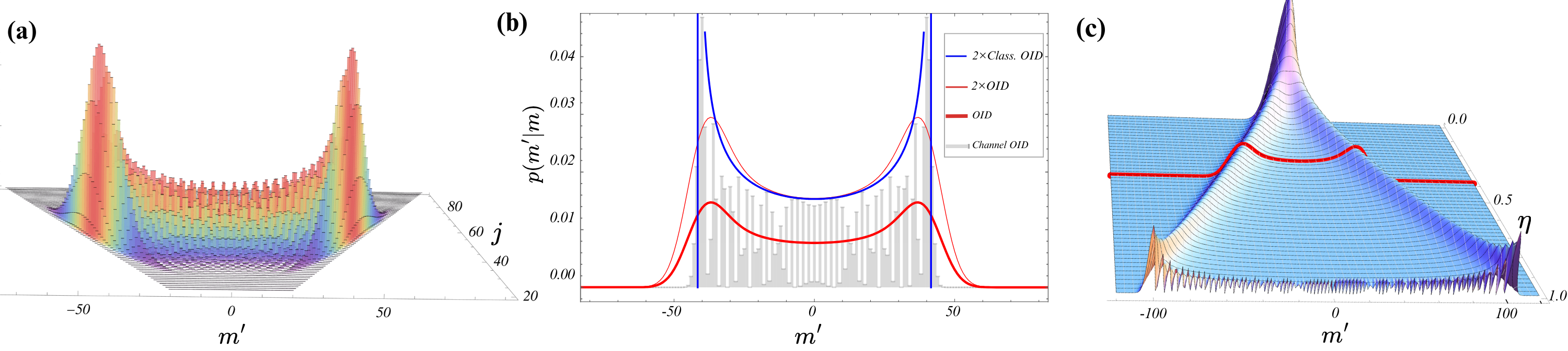
Figure 3: (a) Joint probability $p(j,m^{\prime}|m)=p(j|m)p(m^{\prime}|j,m)$, the summand of Eq. (9) for the OID, as a function of $j$ and $m^{\prime}$ for $n=240$, $m=0$, $\theta=\frac{\pi}{3}$, $\eta=0.4$, showing concentration around $j^{*}=48$. (b) Comparison between the resulting OID $p(m^{\prime}|m)$, the dominant channel OID $p(m^{\prime}|j^{*},m)$ and the classical OID (see Eq. (21)) for the same parameters as in (a). The classical and quantum OID’s are shown scaled by a factor of $2$ to compare with the envelope of $p(m^{\prime}|j^{*},m)$. (c) OID as a function of $\eta$ and $m^{\prime}$ with $n$, $m$ and $\theta$ as in (a) and (b), with the case for $\eta=0.4$ indicated in red.

To understand the large-$n$ behavior of the OID, we analyze the asymptotics of the channel probabillity $p(j|m)$ and the channel OID $p(m^{\prime}|j,m)$. For the latter, we write $p(m^{\prime}|j,m)=|d^{j}_{m^{\prime}m}(\theta)|^{2}$ and following ref. [24], we use the fact that the Wigner small-$d$ matrix elements admit a WKB approximation with an oscillatory “classical” regime and an exponentially decaying regime determined by the sign of

$$R^{j}_{m^{\prime}m}=(J^{2}-m^{2})\sin^{2}\theta-(m^{\prime}-m\cos\theta)^{2}$$ (17)

where $J=\frac{1}{2}+j$ and $R^{j}_{m^{\prime}m}>0$ corresponds to the classical region. In this region $d^{j}_{m^{\prime}m}$ takes the WKB form

$$d^{j}_{m^{\prime}m}(\theta)=\frac{(-1)^{j}\sqrt{2/\pi}}{|R^{j}_{m^{\prime}m}|^{1/4}}\cos(JS^{j}_{m^{\prime}m}-\frac{\pi}{4}),$$ (18)

where $S^{j}_{m^{\prime}m}$ and $R^{j}_{m^{\prime}m}$ are related by $J\frac{\partial^{2}S}{\partial m\partial m^{\prime}}=1/\sqrt{R}$. Thus, as a function of $m^{\prime}$, $p(m^{\prime}|j,m)$ shows oscillations with $O(1)$ fringe separation at the center; as illustrated by the gray histogram in Fig. 3 (b) these oscillations are modulated by an envelope $\propto(R^{j}_{m^{\prime}m})^{-1/2}$ with its minimum at $\langle m^{\prime}\rangle=m\cos\theta$, and peaks around the classical turning points

$$m^{\prime}_{\pm}=m\cos\theta\pm\sqrt{J^{2}-m^{2}}\sin\theta.$$ (19)

Thus $p(m^{\prime}|j,m)$ has an $O(j)$ width, in stark contrast with the $O(\sqrt{j})$ width expected from $2j$ independent events.

Proceeding with the channel probability asymptotics, we find that as $n\rightarrow\infty$ with $j$ and $m$ growing proportionately, the distribution $p(j|m)$ becomes sharply peaked around a certain value $j^{*}$ that depends on $\eta$ and $m$, with an $O(\sqrt{n})$ width. Introducing scaled variables $\overline{\jmath}:=j/n$ and $\overline{m}:=m/n$, we find that $p(j|m)$ follows a large deviations principle $p(j|m)\sim e^{-nr(\overline{\jmath})}$ [25, 26] and therefore concentrates at the value of $\overline{\jmath}$ where rate function $r(\overline{\jmath})=-\lim_{n\rightarrow\infty}\frac{1}{n}\ln p(n\overline{\jmath}|n\overline{m})$ attains its minimum $\ \overline{\jmath}^{*}\in[1/2,\overline{m}]$, which is given by

$$\overline{\jmath}^{*}=\sqrt{\frac{\eta^{2}}{4}+(1-\eta^{2})\overline{m}^{2}}.$$ (20)

As expected, $j^{*}=n\overline{\jmath}^{*}$ is $n/2$ when $\eta=1$; the value $j^{*}=|m|$ for $\eta=0$ is explained from the fact that $2|m|$ indistinguishable photons remain at one of the ports when the maximum number $\min(n_{1},n_{2})$ of singlets has been exhausted.

Combining channel probability and channel OID asymptotics, together with our previous interpretation of the spin-$j$ channels, we arrive at a compelling picture to explain the OID asymptotic behavior. From the concentration of measure of $p(j|m)$, only channels with $|\overline{\jmath}-\overline{\jmath}^{*}|\sim\Delta j=O(n^{-1/2})$ contribute significantly to the sum in Eq. (9). The fact that $\Delta j/j^{*}\sim O(n^{-1/2})$ implies that when $n\rightarrow\infty$, a sharply-defined fraction $2\overline{\jmath}^{*}$ of the photons behave as indistinguishable particles, with the remaining fraction $1-2\overline{\jmath}^{*}$ evenly distributed between the two output ports as singlets.

The shape of the OID is obtained from the channel OIDs with $|\overline{\jmath}-\overline{\jmath}^{*}|\sim\Delta j$, which in terms of scaled variables $\overline{m}$, share the same envelope, up to $O(n^{-1/2})$ corrections. However, for adjacent values of $j$, the fringe patterns in $p(m^{\prime}|j,m)$ show relative displacements of the order of half a fringe. Therefore, as illustrated in Fig. 3 (a) and (b), the fringe patterns are “washed out” in the channel average and only appear when $\eta\sim 1$. Consequently, in the large-$n$ limit, the resulting shape of $p(m^{\prime}|m)$ is essentially the doubly-humped shape of the envelope of $p(m^{\prime}|j^{*},m)$. In particular, in the classical region

$$p(m^{\prime}|m)\propto\frac{1}{\sqrt{\eta^{2}\left(\frac{1}{4}-\overline{m}^{2}\right)\sin^{2}\theta-(\overline{m}^{\prime}-\overline{m}\cos\theta)^{2}}},$$ (21)

as depicted in Fig. 3 (b).

Similarly to the indistinguishable case[7, 11], the OID $p(m^{\prime}|m)$ is in direct correspondence with the classical OID of the output intensities from two beams with random relative phases impinging on the BS, but now exhibiting classical partial indistinguishability, say due to non-parallel polarizations. To see this, suppose two waves of the same frequency impinge on the BS, with electric field amplitudes described by vectors $\boldsymbol{E}_{1}\propto\sqrt{n_{1}}\boldsymbol{\varepsilon}_{1}$, and $\boldsymbol{E}_{2}\propto\sqrt{n_{2}}\boldsymbol{\varepsilon}_{2}e^{i\phi}$, where the $n_{a}$ are the intensities, $\boldsymbol{\varepsilon}_{a}$ are normalized polarization vectors, and $\phi$ the relative phase. After passing through the BS, the output fields satisfy $\boldsymbol{E}_{i}^{\prime}=\sum_{j}U_{ij}\mathcal{R}_{ij}\boldsymbol{E}_{j}$ where the $\mathcal{R}_{ij}$ are polarization rotation matrices preserving the inner product $\boldsymbol{\varepsilon_{1}}^{*}\cdot\boldsymbol{\varepsilon_{2}}$. The outgoing intensities are then given by $n_{a}^{\prime}=|\boldsymbol{E}_{a}^{\prime}|^{2}$, and the output imbalance $m^{\prime}=(n_{1}^{\prime}-n_{2}^{\prime})/2$, as a function of the relative phase, is

$$m^{\prime}(\phi)=m\cos\theta+\eta\sqrt{\frac{n^{2}}{4}-m^{2}}\sin\theta\cos(\phi-\chi),$$ (22)

where $n$ is the total intensity, $\chi=\arg\boldsymbol{\varepsilon_{1}}^{*}\cdot\boldsymbol{\varepsilon_{2}}$, and $\eta:=|\boldsymbol{\varepsilon_{1}}^{*}\cdot\boldsymbol{\varepsilon_{2}}|$. Thus, as $\phi$ is varied, the classical output imbalance oscillates about a mean value $\langle m^{\prime}\rangle=m\cos\theta$ with amplitude $\eta\sqrt{\frac{n^{2}}{4}-m^{2}}\,\sin\theta$. If $\phi$ is now uniformly randomized, the resulting probability distribution for $m^{\prime}$ is exactly the right hand side of Eq. (21), with a proportionality constant of $n/\pi$. Therefore, the OID is centered at the classical mean imbalance and is peaked at the minimum and maximal values of $m^{\prime}(\phi)$. Beyond the classical turning points, the exponential fall-off of the OID may differ somewhat from that of the dominant channel OID. The explanation can be appreciated from Fig. 3(a): in the $(m,j)$ plane, the turning-point positions for $|j-j^{*}|\sim\Delta j$ vary approximately linearly, with their height modulated by the Gaussian shape of $p(j|m)$. Thus these turning-points present a rotated Gaussian profile that distort the tails of the OID after marginalizing to $p(m^{\prime}|m)$.

The $\eta$ dependence of the OID is illustrated in Fig. 3 (c). The maximum width is obtained at $\eta=1$, where the OID shows its full WKB form with interference fringes in the classical region. As $\eta$ decreases, the fringes disappear and the peak separation decreases linearly with $\eta$ until the peaks coalesce into a single one, which corresponds classically to the loss of interference for orthogonal polarizations. In the quantum setting, the peak coalescence signals a transition from a multiphotonic correlated scenario to an independent photon regime. The OID for $\eta=0$ can be explained in terms of $n$ i.i.d. samples of a classical binary symmetric channel (BSC) [27] with error probability $f=\sin^{2}\frac{\theta}{2}$. The resulting OID in this case is centered at $\langle m^{\prime}\rangle=m\cos\theta$ with variance $\langle\Delta m^{\prime 2}\rangle=\frac{n}{4}\sin^{2}\theta\,$ and is approximately Gaussian for large $n$. Hence, one expects a transition when the $\propto n\eta$ width of the quantum OID becomes comparable with the $\propto\sqrt{n}$ width of the BSC distribution. This suggests a critical value, $\eta_{c}$, scaling as $\eta_{c}\sim n^{-1/2}$, a scaling that we have observed numerically.

Finally, in response to the question posed in the introduction, we have shown a coexistence between the classical wave-like and the quantum multiphotonic notions of interference in the asymptotic analysis of the quantum beam splitter. While the asymptotic form of the OID reproduces its classical counterpart, its granular interpretation comes from the multiphotonic interference of a well-defined fraction of perfectly indistinguishable photons, which is determined by combinatorial functions and the degree of indistinguishability. It would be interesting to further investigate the extension of our analysis to the case of more than two ports.