Adaptive Anytime Multi-Agent Path Finding Using
Bandit-Based Large Neighborhood Search
Abstract
Anytime multi-agent path finding (MAPF) is a promising approach to scalable path optimization in large-scale multi-agent systems. State-of-the-art anytime MAPF is based on Large Neighborhood Search (LNS), where a fast initial solution is iteratively optimized by destroying and repairing a fixed number of parts, i.e., the neighborhood of the solution, using randomized destroy heuristics and prioritized planning. Despite their recent success in various MAPF instances, current LNS-based approaches lack exploration and flexibility due to greedy optimization with a fixed neighborhood size which can lead to low-quality solutions in general. So far, these limitations have been addressed with extensive prior effort in tuning or offline machine learning beyond actual planning. In this paper, we focus on online learning in LNS and propose Bandit-based Adaptive LArge Neighborhood search Combined with Exploration (BALANCE). BALANCE uses a bi-level multi-armed bandit scheme to adapt the selection of destroy heuristics and neighborhood sizes on the fly during search. We evaluate BALANCE on multiple maps from the MAPF benchmark set and empirically demonstrate performance improvements of at least 50% compared to state-of-the-art anytime MAPF in large-scale scenarios. We find that Thompson Sampling performs particularly well compared to alternative multi-armed bandit algorithms.
1 Introduction
A wide range of real-world applications like goods transportation in warehouses, search and rescue missions, and traffic management can be formulated as Multi-Agent Path Finding (MAPF) problem, where the goal is to find collision-free paths for multiple agents with each having an assigned start and goal location. Finding optimal solutions, w.r.t. minimal flowtime or makespan is NP-hard, which limits scalability of most state-of-the-art MAPF solvers (Ratner and Warmuth 1986; Yu and LaValle 2013; Sharon et al. 2012).
Anytime MAPF based on Large Neighborhood Search (LNS) is a popular approach to finding fast and near-optimal solutions to the MAPF problem within a fixed time budget (Li et al. 2021). Given an initial feasible solution and a set of destroy heuristics, LNS iteratively destroys and replans so-called neighborhoods of the solution, i.e., a fixed number of paths, until the time budget runs out. MAPF-LNS represents the current state-of-the-art in anytime MAPF and has been experimentally shown to scale up to large-scale scenarios with hundreds of agents (Li et al. 2021). Due to its increasing popularity, several extensions have been recently proposed like fast local repairing, integration of primal heuristics, or machine learning-guided neighborhood selection (Huang et al. 2022; Li et al. 2022; Lam et al. 2023).
However, MAPF-LNS and its variants currently suffer from two limitations that can lead to low-quality solutions in general:
-
1.
The neighborhood size is typically fixed, which limits the flexibility of the optimization process, thus possibly affecting the solution quality, especially for a large number of agents (Li et al. 2021). Therefore, prior tuning is required – in addition to the actual LNS procedure – to obtain good solutions.
-
2.
Roulette wheel selection is commonly used to execute and adapt the destroy heuristic selection to determine the neighborhood (Mara et al. 2022; Li et al. 2021). During optimization, roulette wheel selection could greedily converge to poor choices due to the lack of exploration. Offline machine learning can guide the selection with solution score prediction but requires sufficient data acquisition and feature engineering (Huang et al. 2022).
In this paper, we address these limitations by proposing Bandit-based Adaptive LArge Neighborhood search Combined with Exploration (BALANCE). BALANCE uses a bi-level multi-armed bandit scheme to adapt the selection of destroy heuristics and neighborhood sizes on the fly during search. Our contributions are as follows:
-
•
We formulate BALANCE as a simple but effective MAPF-LNS framework with an adaptive selection of destroy heuristics and neighborhood sizes during search.
-
•
We propose and discuss three concrete instantiations of BALANCE based on roulette wheel selection, UCB1, and Thompson Sampling, respectively.
-
•
We evaluate BALANCE on multiple maps from the MAPF benchmark set and empirically demonstrate cost improvements of at least 50% compared to state-of-the-art anytime MAPF in large-scale scenarios. We find that Thompson Sampling performs particularly well compared to alternative multi-armed bandit algorithms.
2 Background
2.1 Multi-Agent Path Finding (MAPF)
We focus on maps as undirected unweighted graphs , where vertex set contains all possible locations and edge set contains all possible transitions or movements between adjacent locations. An instance consists of a map and a set of agents with each agent having a start location and a goal location .
MAPF aims to find a collision-free plan for all agents. A plan consists of individual paths per agent , where , , , and is the length or travel distance of path . The delay of path is defined by the difference of path length and the length of the shortest path from to w.r.t. map .
In this paper, we consider vertex conflicts that occur when two agents and occupy the same location at time step and edge conflicts that occur when two agents and traverse the same edge in opposite directions at time step (Stern et al. 2019). A plan is a solution, i.e., feasible, when it does not have any vertex or edge conflicts. Our goal is to find a solution that minimizes the flowtime which is equivalent to minimizing the sum of delays . We use the sum of delays or (total) cost as the primary performance measure in our evaluations.
2.2 Anytime MAPF with LNS
Anytime MAPF searches for solutions within a given time budget. The solution quality monotonically improves with increasing time budget (Cohen et al. 2018; Li et al. 2021).
MAPF-LNS based on Large Neighborhood Search (LNS) is the current state-of-the-art approach to anytime MAPF and is shown to scale up to large-scale scenarios with hundreds of agents (Huang et al. 2022; Li et al. 2021). Starting with an initial feasible plan , e.g., found via prioritized planning (PP) from (Silver 2005), MAPF-LNS iteratively modifies by destroying paths, i.e., the neighborhood . The destroyed neighborhood is then repaired or replanned using PP to quickly generate a new solution . If the new cost is lower than the previous cost , then is replaced by , and the search continues until the time budget runs out. The result of MAPF-LNS is the last accepted solution with the lowest cost so far.
MAPF-LNS uses a set of three destroy heuristics , namely a random uniform selection of paths, an agent-based heuristic, and a map-based heuristic (Li et al. 2021). The agent-based heuristic generates the neighborhood, including the path of agent with the current maximum delay and other paths (determined via random walks) that prevent from achieving a lower delay. The map-based heuristic randomly chooses a vertex with a degree greater than 2 and generates a neighborhood of paths containing .
MAPF-LNS uses a selection algorithm like roulette wheel selection to choose destroy heuristics by maintaining updatable weights or some statistics for all destroy heuristics (Ropke and Pisinger 2006; Li et al. 2021). All weights or statistics used by to select a destroy heuristic are denoted by , which could represent, e.g., the average cost improvement or the selection count per destroy heuristic . The statistics will be further explained in Section 4.2 as the concrete definition depends on .
2.3 Multi-Armed Bandits
Multi-armed bandits (MABs) or simply bandits are fundamental decision-making problems, where an MAB or selection algorithm repeatedly chooses an arm among a given set of arms or options to maximize an expected reward of a stochastic reward function , where is a random variable with an unknown distribution . To solve an MAB, one has to determine an optimal arm , which maximizes the expected reward . The MAB algorithm has to balance between sufficiently exploring all arms to accurately estimate via statistics and to exploit its current estimates by greedily selecting the arm with the currently highest estimate of . This is known as the exploration-exploitation dilemma, where exploration can find arms with higher rewards but requires more time for trying them out, while exploitation can lead to fast convergence but possibly gets stuck in a poor local optimum. In this paper, we will cover roulette wheel selection, UCB1, and Thompson Sampling as concrete MAB algorithms and further explain them in Section 4.2.
3 Related Work
3.1 Multi-Armed Bandits for LNS
In recent years, MABs have been used as adaptive meta-controllers to tune learning and optimization algorithms on the fly (Schaul et al. 2019; Badia et al. 2020; Hendel 2022). Besides roulette wheel selection, UCB1 and -greedy are commonly used for destroy heuristic selection in LNS in the context of mixed integer programming, vehicle routing, and scheduling problems with fixed neighborhood sizes (Chen et al. 2016; Chen and Bai 2018; Chmiela et al. 2023). (Hendel 2022) adapts the neighborhood size for mixed integer programming using a mutation-based approach inspired by evolutionary algorithms (Rothberg 2007). Most works use rather complex rewards that are composed of multiple weighted terms with several tunable hyperparameters. We focus on MAPF problems and propose a bi-level MAB scheme to adapt the selection of destroy heuristics and neighborhood sizes, which is simple to use without any additional mechanisms like mutation. Our approach uses the cost improvement as a reward, which simply represents the cost difference between two solutions w.r.t. the original objective of MAPF without depending on any additional weighted term that requires prior tuning. To the best of our knowledge, our work first effectively applies Thompson Sampling to anytime MAPF in addition to more common MAB algorithms like UCB1 and roulette wheel selection.
3.2 Multi-Armed Bandits in Anytime Planning
MABs are popular in anytime planning algorithms, especially in single-agent Monte Carlo planning (Kocsis and Szepesvári 2006; Silver and Veness 2010). Monte-Carlo Tree Search (MCTS) is the state-of-the-art framework of current Monte Carlo planning algorithms which uses MABs to traverse a search tree within a limited time budget (Kocsis and Szepesvári 2006; Silver and Veness 2010). UCB1 is most commonly used, but Thompson Sampling has also gained attention in the last few years due to its effectiveness in domains of high uncertainty (Bai, Wu, and Chen 2013; Bai et al. 2014; Phan et al. 2019a, b). As MABs have been shown to converge to good decisions within short-time budgets, we use MABs in our adaptive multi-agent path finding setting. Inspired by the latest progress in Monte Carlo planning (Świechowski et al. 2023), we intend to employ more sophisticated MAB algorithms like Thompson Sampling to anytime MAPF to improve exploration and performance.
3.3 Machine Learning in Anytime MAPF
Machine learning has been used in MAPF to directly learn collision-free path finding, to guide node selection in search trees, or to select appropriate MAPF algorithms for certain maps (Sartoretti et al. 2019; Kaduri, Boyarski, and Stern 2020; Huang, Dilkina, and Koenig 2021). MAPF-ML-LNS is an anytime MAPF approach that extends MAPF-LNS with a learned score predictor for neighborhood selection as well as a random uniform selection of the neighborhood size . The predictor is trained offline on pre-collected data from previous MAPF runs (Huang et al. 2022). The score predictor generalizes to some degree but is fixed after training; therefore, not being able to adapt during search, which limits flexibility. MAPF-ML-LNS depends on extensive prior effort like data acquisition, model training, and feature engineering for meaningful score learning. We propose an online learning approach to adaptive MAPF-LNS using MABs. The MABs can be trained on the fly with data directly obtained from the LNS without any prior data acquisition. Since MABs only learn from scalar rewards, there is no need for expensive feature engineering, simplifying our approach and easing application to other domains.
4 Bandit-Based Adaptive MAPF-LNS
We now introduce Bandit-based Adaptive LArge Neighborhood search Combined with Exploration (BALANCE) as a simple but effective LNS framework for adaptive MAPF.
4.1 Formulation
BALANCE uses a bi-level MAB scheme to adapt the selection of destroy heuristics and neighborhood sizes on the fly during search. The first level consists of a single MAB, called -Bandit with arms, which selects a destroy heuristic . The second level consists of so-called -Bandits with arms. Each -Bandit conditions on a destroy heuristic choice and determines the corresponding neighborhood size 111The set of neighborhood size options can be defined arbitrarily. For simplicity, we focus on sets consisting of powers of two. based on an exponent selection . The bi-level MAB scheme is shown in Figure 1.
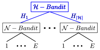
BALANCE first selects a destroy heuristic with the top-level -Bandit based on its current statistics . The selected destroy heuristic determines the corresponding bottom-level -Bandit, which is used to select an exponent based on its current conditional statistics . The neighborhood size is then determined by . After evaluating the total cost of the new solution , i.e. the sum of delays, the statistics of the top-level -Bandit and corresponding bottom-level -Bandit are updated incrementally. The MAB reward for the update is defined by the cost improvement of the new solution compared to the previous one (Li et al. 2021).
The full formulation of BALANCE is provided in Algorithm 1, where represents the instance to be solved, represents the MAB algorithm for the bi-level scheme, and represents the number of neighborhood size options.
4.2 Instantiations
In the following, we describe three concrete MAB algorithms to implement the bi-level scheme in Figure 1. The definition of the statistics depends on the MAB algorithm.
Roulette Wheel Selection
selects an arm with a probability of , where is the sum of rewards or weight and is the selection count of arm . Statistics consists of all weights , which can be updated incrementally after each iteration (Goldberg 1988).
UCB1
selects arms by maximizing the upper confidence bound of rewards , where is the average reward of arm , is an exploration constant, is the total number of arm selections, and is the selection count of arm . The second term represents the exploration bonus, which becomes smaller with increasing (Auer, Cesa-Bianchi, and Fischer 2002). Statistics consists of all average rewards and selection counts .
Thompson Sampling
uses a Bayesian approach to balance between exploration and exploitation of arms (Thompson 1933). We focus on a generalized variant of Thompson Sampling, which works for arbitrary reward distributions by assuming that follows a Normal distribution with unknown mean and precision , where is the variance (Bai, Wu, and Chen 2013; Bai et al. 2014). follows a Normal Gamma distribution with , , and . The distribution over is a Gamma distribution and the conditional distribution over given is a Normal distribution . Given a prior distribution and observed rewards , the posterior distribution is defined by , where , , , and . is the observed average reward in and is the variance. The posterior is inferred for each arm to sample an estimate of the expected reward . The arm with the highest estimate is selected. Statistics consists of all average rewards , average of squared rewards , and selection counts .
4.3 Conceptual Discussion
As MAB algorithms balance between exploration and exploitation to quickly find optimal choices, we believe that they are naturally suited to enhance MAPF-LNS with self-adaptive capabilities. According to previous works on MAB-based tree search, BALANCE can provably converge to an optimal destroy heuristic and neighborhood size choice with sufficient exploration if there is a stationary optimum (Kocsis and Szepesvári 2006; Bai et al. 2014). Otherwise, non-stationary MAB techniques are required, which we defer to as future work (Garivier and Moulines 2008). Depending on the choice of , BALANCE maintains MABs in total. Since can be updated incrementally for any quantity like arm selection counts or average rewards , the bi-level MAB scheme can be updated in constant time thus introducing negligible overhead to the LNS (as replanning of neighborhoods requires significantly more compute).
Roulette wheel selection is the simplest method to implement because it only uses the weights as the sum of rewards. However, it could lack exploration in the long run since arms with small weights are likely to be neglected or forgotten over time. UCB1 accommodates this issue by introducing an exploration bonus that explicitly considers the selection count of arms . Arms that are selected less over time will have a larger exploration bonus and are therefore more incentivized for selection, depending on the choice of exploration constant . Thompson Sampling is a randomized algorithm whose initial exploration depends on prior parameters, i.e., , , , and thus being more complex than the other MAB approaches. However, previous works report that using prior distributions that are close to a uniform distribution is sufficient in most cases without requiring extensive tuning (Bai, Wu, and Chen 2013; Bai et al. 2014).
Adaptation in MAPF-LNS can be regarded as stochastic optimization problem, since all destroy heuristics defined by (Li et al. 2021) are randomized. Therefore, uncertainty-based methods like Thompson Sampling seem promising for this setting as reported in (Chapelle and Li 2011; Kaufmann, Korda, and Munos 2012; Bai et al. 2014).
Alternatively to the proposed bi-level MAB scheme, a single MAB can be employed to directly search the joint arm space of . While this approach would basically solve the same problem, the joint arm space scales quadratically, which could lead to low-quality solutions, if the time budget is very restricted. The bi-level scheme mitigates the scalability issue by first selecting a destroy heuristic (Section 5.3 indicates that performance is more sensitive to ) before deciding on the neighborhood size (whose quality depends on the choice of ).
5 Experiments
5.1 Setup
Maps
We evaluate BALANCE on five maps from the MAPF benchmark set of (Stern et al. 2019), namely (1) a random map (random-32-32-10), (2) a warehouse map (warehouse-10-20-10-2-1), (3) two game maps ost003d and (4) den520d as well as (5) a city map (Paris_1_256). All maps have different sizes and structures and are the same as used in (Huang et al. 2022) for comparability with state-of-the-art anytime MAPF as presented below. We conduct all experiments on the available 25 random scenarios per map.
Anytime MAPF Algorithms
We implemented222Code available at github.com/thomyphan/anytime-mapf. different variants of BALANCE using Thompson Sampling (with , , , ), UCB1 (with ), and roulette wheel selection. Each BALANCE variant is denoted by BALANCE (X), where X is the concrete MAB algorithm (or just random uniform sampling) used for our bi-level scheme in Figure 1. Unless stated otherwise, we always use the destroy heuristics from (Li et al. 2021) and set such that the neighborhood size is chosen from 333Even though previous works (Li et al. 2021, 2022) already indicate good values for fixed neighborhood sizes , we keep optimizing our MABs on a broader set of options to confirm convergence to adequate choices without assuming any prior knowledge.. Our BALANCE implementation is based on the public code of (Li et al. 2022) and uses its default configuration unless stated otherwise.
We determine the Empirically Best Choice, where we run a grid search over all destroy heuristics and neighborhood size options to compare with a pre-tuned LNS without any adaptation.
To directly compare BALANCE with MAPF-LNS and MAPF-ML-LNS, as state-of-the-art approaches, we take the performance values reported in (Huang et al. 2022), running our experiments on the same hardware specification. We also compare with a single-MAB approach that optimizes over the Joint Arm Space using Thompson Sampling.
Compute Infrastructure
All experiments were run on a x86_64 GNU/Linux (Ubuntu 18.04.5 LTS) machine with i7 @ 2.4 GHz CPU and 16 GB RAM, as in (Huang et al. 2022).
5.2 Experiment – BALANCE Convergence
Setting
To assess convergence w.r.t. time budget, we run BALANCE (Thompson), BALANCE (UCB1), BALANCE (Roulette), and BALANCE (Random) on the random and city map with and agents respectively.
Results
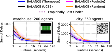
The results are shown in Figure 2. With increasing time budget, all BALANCE variants converge to an average sum of delays close to the empirically best choice. All MAB-enhanced variants converge faster than BALANCE (Random). BALANCE (Thompson) performs best in both maps, especially when the time budget is low.
Discussion
The results show that any version of BALANCE is able to perform well with an increasing time budget. Given a sufficient time budget, all versions are able to keep up with the empirically best choice through online learning without running a prior grid search that requires roughly times the compute of any BALANCE variant in total. Thompson Sampling performs particularly well, presumably due to the inherent uncertainty exhibited by the randomized destroy heuristics.
5.3 Experiment – BALANCE Exploration
Setting
Next, we evaluate the explorative behavior of BALANCE (Thompson), BALANCE (UCB1), and BALANCE (Roulette) on the random, ost003d, and city map after 128 seconds of LNS runtime. We also evaluate the progress of MAB choice over time for BALANCE (Thompson) and BALANCE (Roulette) in the ost003d map.
Results
The final relative frequencies of MAB choices are displayed as heatmaps in Figure 3. The empirically best destroy heuristics and neighborhood sizes are highlighted by magenta dashed boxes. BALANCE (UCB1) and BALANCE (Roulette) strongly prefer the random destroy heuristic, while the preferred neighborhood size depends on the actual map. BALANCE (Thompson) also prefers the random destroy heuristic to some degree but still explores other heuristics, mainly with neighborhood sizes . Compared to the other variants, BALANCE (Thompson) explores more regions where either the destroy heuristic or the neighborhood size is empirically best, at least.
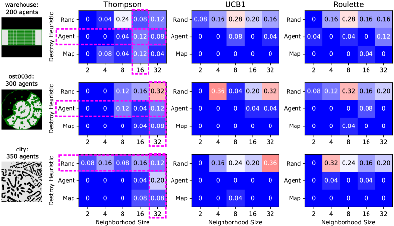
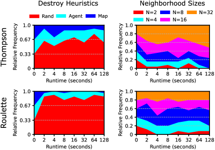
Figure 4 shows the average progress of the chosen destroy heuristic and neighborhood size during search for Thompson Sampling and Roulette in the ost003d map. While Roulette quickly converges to the random heuristic, Thompson Sampling adapts its preferences through continuous exploration. Thompson Sampling mostly prefers the largest neighborhood size over time, whereas Roulette almost uniformly chooses over time with a slight preference toward .
Discussion
None of the BALANCE variants clearly converges to the empirically best choice, which could be due to a short time budget, marginal improvement over time, or potential non-stationarity of the actual optimal choice. Nevertheless, Figure 3 suggests that Thompson Sampling performs more focused exploration than any other MAB.
5.4 Experiment – Neighborhood Size Options
Setting
We run BALANCE (Thompson), BALANCE (UCB1), BALANCE (Roulette), and BALANCE (Random) with different neighborhood size options by varying , i.e., the number of exponents to determine the neighborhood size . The same maps and number of agents as above are used with a time budget of 128 seconds. We additionally evaluate with a doubled number of agents per map.
Results
The results are shown in Figure 5. All approaches significantly improve when the number of options is increased to with marginal to no improvement afterward. BALANCE (Thompson) and BALANCE (Random) benefit the most from the increase of except in the city map with 700 agents, where BALANCE (UCB1) keeps up with BALANCE (Thompson).
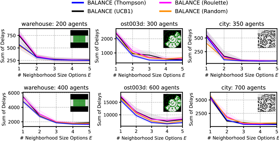
Discussion
Since Thompson Sampling and random uniform explore more than UCB1 and Roulette, they can better leverage the neighborhood size options. The results indicate that neighborhood size adaptation and the sufficient availability of options can significantly affect performance. However, the neighborhood size also affects the amount of compute for replanning, which explains why BALANCE (Random) performs worse in ost003d when .
5.5 Experiment – State-of-the-Art Comparison
Setting
We run BALANCE (Thompson), BALANCE (UCB1), BALANCE (Roulette), and Joint Arm Space (Thompson) on the random, warehouse, ost003d, den520d, and city map with different numbers of agents . For direct comparability with MAPF-LNS and MAPF-ML-LNS, we set the time budget to 60 seconds (Huang et al. 2022). Since no error or deviation bars are reported in (Huang et al. 2022), we only show the average performance of MAPF-LNS and MAPF-ML-LNS as dashed lines.
Results
The results are shown in Figure 6. All BALANCE variants and Joint Arm Space (Thompson) significantly outperform MAPF-LNS and MAPF-ML-LNS by at least 50% when . In the random, ost003d, and city map, BALANCE (Thompson) slightly outperforms the other BALANCE variants. Joint Arm Space (Thompson) is consistently outperformed by the BALANCE variants.
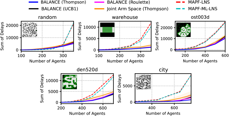
Discussion
The experiment demonstrates that BALANCE effectively mitigates the limitations of state-of-the-art anytime MAPF regarding fixed neighborhood sizes and the lack of exploration in roulette wheel selection, especially in instances with a large number of agents . While Thompson Sampling seemingly performs best in most cases, using BALANCE with any MAB algorithm is generally beneficial to improve performance. As discussed in Section 4.3, our bi-level MAB scheme can outperform joint arm space alternatives when the time budget is very restricted due to meaningful decomposition, which is confirmed in all tested maps. However, since Joint Arm Space (Thompson) also outperforms the state-of-the-art, we suggest that bandit-based adaptation in MAPF-LNS is generally promising.
6 Conclusion
We presented BALANCE, an LNS framework using a bi-level multi-armed bandit scheme to adapt the selection of destroy heuristics and neighborhood sizes during search.
Our experiments show that BALANCE offers a simple but effective framework for adaptive anytime MAPF, which is able to significantly outperform state-of-the-art anytime MAPF without requiring extensive prior efforts like neighborhood size tuning, data acquisition, or feature engineering. Sufficient availability of neighborhood size options is important to provide enough room for adaptation at the potential cost of runtime due to increasing replanning effort. Thompson Sampling is a promising choice for most scenarios due to the inherent uncertainty of the randomized destroy heuristics and its ability to explore promising choices.
Future work includes the investigation of non-stationary MAB approaches and online learnable destroy heuristics.
Acknowledgements
The research at the University of Southern California was supported by the National Science Foundation (NSF) under grant numbers 1817189, 1837779, 1935712, 2121028, 2112533, and 2321786 as well as a gift from Amazon Robotics. The views and conclusions contained in this document are those of the authors and should not be interpreted as representing the official policies, either expressed or implied, of the sponsoring organizations, agencies, or the U.S. government.
References
- Auer, Cesa-Bianchi, and Fischer (2002) Auer, P.; Cesa-Bianchi, N.; and Fischer, P. 2002. Finite-Time Analysis of the Multiarmed Bandit Problem. Machine learning, 47(2-3): 235–256.
- Badia et al. (2020) Badia, A. P.; Piot, B.; Kapturowski, S.; Sprechmann, P.; Vitvitskyi, A.; Guo, Z. D.; and Blundell, C. 2020. Agent57: Outperforming the Atari Human Benchmark. In International conference on machine learning, 507–517. PMLR.
- Bai, Wu, and Chen (2013) Bai, A.; Wu, F.; and Chen, X. 2013. Bayesian Mixture Modelling and Inference based Thompson Sampling in Monte-Carlo Tree Search. In Advances in Neural Information Processing Systems, 1646–1654.
- Bai et al. (2014) Bai, A.; Wu, F.; Zhang, Z.; and Chen, X. 2014. Thompson Sampling based Monte-Carlo Planning in POMDPs. In Proceedings of the Twenty-Fourth International Conferenc on International Conference on Automated Planning and Scheduling, 29–37. AAAI Press.
- Chapelle and Li (2011) Chapelle, O.; and Li, L. 2011. An Empirical Evaluation of Thompson Sampling. In Advances in neural information processing systems, 2249–2257.
- Chen and Bai (2018) Chen, B.; and Bai, R. 2018. A Reinforcement Learning Based Variable Neighborhood Search Algorithm for Open Periodic Vehicle Routing Problem with Time Windows.
- Chen et al. (2016) Chen, Y.; Cowling, P. I.; Polack, F. A. C.; and Mourdjis, P. 2016. A Multi-Arm Bandit Neighbourhood Search for Routing and Scheduling Problems.
- Chmiela et al. (2023) Chmiela, A.; Gleixner, A.; Lichocki, P.; and Pokutta, S. 2023. Online Learning for Scheduling MIP Heuristics. In International Conference on Integration of Constraint Programming, Artificial Intelligence, and Operations Research, 114–123. Springer.
- Cohen et al. (2018) Cohen, L.; Greco, M.; Ma, H.; Hernández, C.; Felner, A.; Kumar, T. S.; and Koenig, S. 2018. Anytime Focal Search with Applications. In IJCAI, 1434–1441.
- Garivier and Moulines (2008) Garivier, A.; and Moulines, E. 2008. On Upper-Confidence Bound Policies for Non-Stationary Bandit Problems. arXiv preprint arXiv:0805.3415.
- Goldberg (1988) Goldberg, D. E. 1988. Genetic Algorithms in Search Optimization and Machine Learning.
- Hendel (2022) Hendel, G. 2022. Adaptive Large Neighborhood Search for Mixed Integer Programming. Mathematical Programming Computation, 1–37.
- Huang, Dilkina, and Koenig (2021) Huang, T.; Dilkina, B.; and Koenig, S. 2021. Learning Node-Selection Strategies in Bounded Suboptimal Conflict-Based Search for Multi-Agent Path Finding. In International Joint Conference on Autonomous Agents and Multiagent Systems (AAMAS).
- Huang et al. (2022) Huang, T.; Li, J.; Koenig, S.; and Dilkina, B. 2022. Anytime Multi-Agent Path Finding via Machine Learning-Guided Large Neighborhood Search. In Proceedings of the 36th AAAI Conference on Artificial Intelligence (AAAI), 9368–9376.
- Kaduri, Boyarski, and Stern (2020) Kaduri, O.; Boyarski, E.; and Stern, R. 2020. Algorithm Selection for Optimal Multi-Agent Pathfinding. In Proceedings of the International Conference on Automated Planning and Scheduling, volume 30, 161–165.
- Kaufmann, Korda, and Munos (2012) Kaufmann, E.; Korda, N.; and Munos, R. 2012. Thompson Sampling: An Asymptotically Optimal Finite-Time Analysis. In International Conference on Algorithmic Learning Theory, 199–213. Springer.
- Kocsis and Szepesvári (2006) Kocsis, L.; and Szepesvári, C. 2006. Bandit based Monte-Carlo Planning. In ECML, volume 6, 282–293. Springer.
- Lam et al. (2023) Lam, E.; Harabor, D.; Stuckey, P. J.; and Li, J. 2023. Exact Anytime Multi-Agent Path Finding Using Branch-and-Cut-and-Price and Large Neighborhood Search. In Proceedings of the International Conference on Automated Planning and Scheduling (ICAPS).
- Li et al. (2021) Li, J.; Chen, Z.; Harabor, D.; Stuckey, P. J.; and Koenig, S. 2021. Anytime Multi-Agent Path Finding via Large Neighborhood Search. In Proceedings of the International Joint Conference on Artificial Intelligence (IJCAI), 4127–4135.
- Li et al. (2022) Li, J.; Chen, Z.; Harabor, D.; Stuckey, P. J.; and Koenig, S. 2022. MAPF-LNS2: Fast Repairing for Multi-Agent Path Finding via Large Neighborhood Search. Proceedings of the AAAI Conference on Artificial Intelligence, 36(9): 10256–10265.
- Mara et al. (2022) Mara, S. T. W.; Norcahyo, R.; Jodiawan, P.; Lusiantoro, L.; and Rifai, A. P. 2022. A Survey of Adaptive Large Neighborhood Search Algorithms and Applications. Computers & Operations Research, 146: 105903.
- Phan et al. (2019a) Phan, T.; Belzner, L.; Kiermeier, M.; Friedrich, M.; Schmid, K.; and Linnhoff-Popien, C. 2019a. Memory Bounded Open-Loop Planning in Large POMDPs using Thompson Sampling. Proceedings of the AAAI Conference on Artificial Intelligence, 33(01): 7941–7948.
- Phan et al. (2019b) Phan, T.; Gabor, T.; Müller, R.; Roch, C.; and Linnhoff-Popien, C. 2019b. Adaptive Thompson Sampling Stacks for Memory Bounded Open-Loop Planning. In Proceedings of the 28th International Joint Conference on Artificial Intelligence, IJCAI-19, 5607–5613. International Joint Conferences on Artificial Intelligence Organization.
- Ratner and Warmuth (1986) Ratner, D.; and Warmuth, M. 1986. Finding a Shortest Solution for the NxN Extension of the 15-Puzzle is Intractable. In Proceedings of the Fifth AAAI National Conference on Artificial Intelligence, AAAI’86, 168–172. AAAI Press.
- Ropke and Pisinger (2006) Ropke, S.; and Pisinger, D. 2006. An Adaptive Large Neighborhood Search Heuristic for the Pickup and Delivery Problem with Time Windows. Transportation science, 40(4): 455–472.
- Rothberg (2007) Rothberg, E. 2007. An Evolutionary Algorithm for Polishing Mixed Integer Programming Solutions. INFORMS Journal on Computing, 19(4): 534–541.
- Sartoretti et al. (2019) Sartoretti, G.; Kerr, J.; Shi, Y.; Wagner, G.; Kumar, T. S.; Koenig, S.; and Choset, H. 2019. PRIMAL: Pathfinding via Reinforcement and Imitation Multi-Agent Learning. IEEE Robotics and Automation Letters, 4(3): 2378–2385.
- Schaul et al. (2019) Schaul, T.; Borsa, D.; Ding, D.; Szepesvari, D.; Ostrovski, G.; Dabney, W.; and Osindero, S. 2019. Adapting Behaviour for Learning Progress. arXiv preprint arXiv:1912.06910.
- Sharon et al. (2012) Sharon, G.; Stern, R.; Felner, A.; and Sturtevant, N. 2012. Conflict-Based Search For Optimal Multi-Agent Path Finding. Proceedings of the AAAI Conference on Artificial Intelligence, 26(1): 563–569.
- Silver (2005) Silver, D. 2005. Cooperative Pathfinding. Proceedings of the AAAI Conference on Artificial Intelligence and Interactive Digital Entertainment, 1(1): 117–122.
- Silver and Veness (2010) Silver, D.; and Veness, J. 2010. Monte-Carlo Planning in Large POMDPs. In Advances in neural information processing systems, 2164–2172.
- Stern et al. (2019) Stern, R.; Sturtevant, N.; Felner, A.; Koenig, S.; Ma, H.; Walker, T.; Li, J.; Atzmon, D.; Cohen, L.; Kumar, T.; et al. 2019. Multi-Agent Pathfinding: Definitions, Variants, and Benchmarks. In Proceedings of the International Symposium on Combinatorial Search, volume 10, 151–158.
- Świechowski et al. (2023) Świechowski, M.; Godlewski, K.; Sawicki, B.; and Mańdziuk, J. 2023. Monte Carlo Tree Search: A Review of Recent Modifications and Applications. Artificial Intelligence Review, 56(3): 2497–2562.
- Thompson (1933) Thompson, W. R. 1933. On the Likelihood that One Unknown Probability exceeds Another in View of the Evidence of Two Samples. Biometrika, 25(3/4): 285–294.
- Yu and LaValle (2013) Yu, J.; and LaValle, S. 2013. Structure and Intractability of Optimal Multi-Robot Path Planning on Graphs. Proceedings of the AAAI Conference on Artificial Intelligence, 27(1): 1443–1449.