Approximation algorithms for noncommutative constraint satisfaction problems

Abstract

We study operator – or noncommutative – variants of constraint satisfaction problems (CSPs). These higher-dimensional variants are a core topic of investigation in quantum information, where they arise as nonlocal games and entangled multiprover interactive proof systems (MIP*). The idea of higher-dimensional relaxations of CSPs is also important in the classical literature. For example since the celebrated work of Goemans and Williamson on $\mathrm{Max}\textit{-}\mathrm{Cut}$, higher dimensional vector relaxations have been central in the design of approximation algorithms for classical CSPs.

We introduce a framework for designing approximation algorithms for noncommutative CSPs. Prior to this work $\mathrm{Max}\textit{-}{2}\textit{-}\mathrm{Lin}({2})$ was the only family of noncommutative CSPs known to be efficiently solvable. This work is the first to establish approximation ratios for a broader class of noncommutative CSPs.

In the study of classical CSPs, $k$-ary decision variables are often represented by $k$-th roots of unity, which generalise to the noncommutative setting as order-$k$ unitary operators. In our framework, using representation theory, we develop a way of constructing unitary solutions from SDP relaxations, extending the pioneering work of Tsirelson on XOR games. Then, we introduce a novel rounding scheme to transform these solutions to order-$k$ unitaries. Our main technical innovation here is a theorem guaranteeing that, for any set of unitary operators, there exists a set of order-$k$ unitaries that closely mimics it. As an integral part of the rounding scheme, we prove a random matrix theory result that characterises the distribution of the relative angles between eigenvalues of random unitaries using tools from free probability.

1 Introduction

1.1 Motivation and Background

$\mathrm{Max}\textit{-}{2}\textit{-}\mathrm{Lin}({k})$ [1, 2, 3] is a class of CSPs that includes the famous Unique-Games problem [5] as well as some well-studied combinatorial optimization problems such as $\mathrm{Max}\textit{-}\mathrm{Cut}({k})$ [6, 7, 8, 2, 9]. Given $N$ variables $x_{1},\ldots,x_{N}$ taking values in $\mathbb{Z}_{k}=\{0,1,\ldots,k-1\}$ and a system of linear equations $x_{j}-x_{i}=c_{ij}$ or linear inequations $x_{j}-x_{i}\neq c_{ij}$ for constants $c_{ij}\in\mathbb{Z}_{k}$, each with an associated weight $w_{ij}\geq 0$, the goal of $\mathrm{Max}\textit{-}{2}\textit{-}\mathrm{Lin}({k})$ is to maximize the total weight of satisfied constraints.

More generally, CSPs are defined with arbitrary constraints on the variables, and $2$-CSPs are the class where each constraint involves only two variables at a time. Because we will only be working with $2$-CSPs in the rest of the paper we simply use the notation $\mathrm{Max}\textit{-}\mathrm{Lin}({k})$ when referring to $\mathrm{Max}\textit{-}{2}\textit{-}\mathrm{Lin}({k})$.

$\mathrm{Unique}\textit{-}\mathrm{Game}({k})$ are those instances of $\mathrm{Max}\textit{-}\mathrm{Lin}({k})$ with only equation constraints. On the other end, instances with only inequation constraints include $\mathrm{Max}\textit{-}\mathrm{Cut}({k})$ problems and their generalisations. In $\mathrm{Max}\textit{-}\mathrm{Cut}({k})$ the goal is to partition the vertices of a graph into $k$ blocks such that the number of edges crossing the blocks is maximized. This problem can be framed as an instance of $\mathrm{Max}\textit{-}\mathrm{Lin}({k})$ by associating a variable $x_{i}$ to every vertex $i$ and a constraint $x_{j}-x_{i}\neq 0$ to every edge $(i,j)$.

In order to express a CSP as a polynomial optimization problem, instead of $\mathbb{Z}_{k}$, we use $k$-th roots of unity $\{1,\omega,\ldots,\omega^{k-1}\}$, where $\omega=e^{\frac{2\pi i}{k}}$. Therefore, we can equivalently state a $\mathrm{Max}\textit{-}\mathrm{Lin}({k})$ instance in multiplicative form where the variables $x_{1},\ldots,x_{n}$ take values that are $k$-th roots of unity, and the constraints are $x_{i}^{-1}x_{j}=\omega^{c_{ij}}$ or $x_{i}^{-1}x_{j}\neq\omega^{c_{ij}}$ for constants $c_{ij}\in\mathbb{Z}_{k}$. This multiplicative framing is also sometimes preferred in the literature, see for example [2]. When $x,y$ are $k$-th roots of unity, the polynomial $\frac{1}{k}\sum_{s=0}^{k-1}\omega^{-cs}x^{-s}y^{s}$ indicates whether the equation $x^{-1}y=\omega^{c}$ is satisfied, since

$$\frac{1}{k}\sum_{s=0}^{k-1}\omega^{-cs}x^{-s}y^{s}=\begin{cases}0&x^{-1}y\neq\omega^{c}\\ 1,&x^{-1}y=\omega^{c}.\end{cases}$$

So, we can frame $\mathrm{Max}\textit{-}\mathrm{Lin}({k})$ as a polynomial optimization problem

maximize: $$\sum_{(i,j)\in\mathcal{E}}\frac{w_{ij}}{k}{\sum_{s=0}^{k-1}\omega^{-c_{ij}s}x_{i}^{-s}x_{j}^{s}}+\sum_{(i,j)\in\mathcal{I}}w_{ij}\big{(}1-\frac{1}{k}{\sum_{s=0}^{k-1}\omega^{-c_{ij}s}x_{i}^{-s}x_{j}^{s}}\big{)}$$ (1.1)

subject to: $$x_{i}^{k}=1\text{ and }x_{i}\in\mathbb{C},$$

where $\mathcal{E}$ is the set of equation constraints and $\mathcal{I}$ is the set of inequation constraints.

$\mathrm{Max}\textit{-}\mathrm{Lin}({k})$ is famously $\mathsf{NP}$-hard [10]. However, efficient approximation algorithms for these problems have long been known. To understand the quality of these approximations, we need the following definition.

Definition 1.1.

The approximation ratio of an algorithm $\mathcal{A}$ for a CSP such as $\mathrm{Max}\textit{-}\mathrm{Lin}({k})$ is the quantity $\inf_{I}\frac{\mathcal{A}(I)}{\operatorname{\mathrm{OPT}}(I)}$ where $I$ ranges over all possible instances of the problem and $\operatorname{\mathrm{OPT}}(I)$ is the optimal value of the instance $I$.

Håstad [11] proves that it is NP-hard to approximate $\mathrm{Max}\textit{-}\mathrm{Cut}$ to a ratio better than $0.94$. In the case of $\mathrm{Max}\textit{-}\mathrm{Lin}({3})$ this inapproximability ratio stands at $\approx 0.944$ [1]. Along these lines, the famous Unique-Games Conjecture (UGC) [5, 3, 4] states that:

Conjecture 1.2 (Unique-Games Conjecture).

For every $\varepsilon>0$, there exists a large enough $k$, such that it is NP-hard deciding whether in a given instance of $\mathrm{Unique}\textit{-}\mathrm{Game}({k})$ at least $1-\varepsilon$ or at most $\varepsilon$ fraction of total weights can be satisfied.

On the positive side, there are a variety of approximation algorithms for $\mathrm{Max}\textit{-}\mathrm{Lin}({k})$ based on semidefinite programming (SDP) relaxations. We will see some of these SDP relaxations in Section 1.2.1. The following definition captures the quality of an SDP relaxation:

Definition 1.3.

The integrality gap of an SDP relaxation for a CSP is $\inf_{I}\frac{\operatorname{\mathrm{OPT}}(I)}{\operatorname{\it\mathrm{SDP}}(I)}$, where the infimum ranges over all instances $I$ of the CSP and $\operatorname{\it\mathrm{SDP}}(I)$ is the optimal value of the SDP on the instance $I$.

For $\mathrm{Max}\textit{-}\mathrm{Cut}\coloneqq\mathrm{Max}\textit{-}\mathrm{Cut}({2})$, the celebrated Goemans-Williamson algorithm [7] gave an approximation ratio of $0.878$. This ratio turned out to be the same as the integrality gap of the SDP relaxation [12]. Frieze and Jerrum [8] gave an approximation ratio of $1-1/k+2(\ln k)/k^{2}$ for $\mathrm{Max}\textit{-}\mathrm{Cut}({k})$ in the limit of large $k$. Khot et al. [3] showed that, assuming UGC, both these results are tight, meaning that there is no efficient algorithm that does better. Goemans and Williamson [2] gave an approximation ratio of $0.836$ for $\mathrm{Max}\textit{-}\mathrm{Cut}({3})$ and $0.793$ for $\mathrm{Max}\textit{-}\mathrm{Lin}({3})$. In particular these establish lower bounds on the integrality gap of the respective SDP relaxations. Moreover, the algorithm for $\mathrm{Max}\textit{-}\mathrm{Cut}({3})$ is tight assuming the “three candidate plurality is stablest” conjecture [3].

We study noncommutative variants of $\mathrm{Max}\textit{-}\mathrm{Lin}({k})$ in this paper. One such variant is obtained from the classical problem by relaxing the commutativity constraint in the polynomial (1.1). This leads us to the following noncommutative polynomial optimization problem

maximize: $$\Big{\|}\sum_{(i,j)\in\mathcal{E}}\frac{w_{ij}}{k}{\sum_{s=0}^{k-1}\omega^{-c_{ij}s}X_{i}^{-s}X_{j}^{s}}+\sum_{(i,j)\in\mathcal{I}}w_{ij}\big{(}1-\frac{1}{k}{\sum_{s=0}^{k-1}\omega^{-c_{ij}s}X_{i}^{-s}X_{j}^{s}}\big{)}\Big{\|}_{\mathrm{op}}$$ (1.2)

subject to: $$X_{i}^{*}X_{i}=X_{i}^{k}=1,$$

where the maximization ranges over all finite-dimensional Hilbert spaces and unitary operators of order $k$ acting on them. Throughout the paper, $\ast$ denotes Hermitian conjugate and $\|\cdot\|_{\mathrm{op}}$ denotes the operator norm. The value of (1.2) is an upper bound on the classical value since (1.1) is the restriction of (1.2) to the one-dimensional Hilbert space. For a discussion of other noncommutative generalisations of classical CSPs, such as the problem known as Quantum $\mathrm{Max}\textit{-}\mathrm{Cut}$, see Section 1.4.4.

It turns out that this noncommutative problem is equivalent to an SDP, so it can be solved efficiently. Furthermore an optimal solution exists in a Hilbert space of dimension $O(N)$. In the special case of $\mathrm{Max}\textit{-}\mathrm{Cut}({k})$, this SDP is the canonical SDP relaxation of the classical problem. This indicates that there is a close relationship between noncommutative CSPs and classical CSPs, that we will elaborate on in Section 1.3. Finally we note that in the special case of Unique-Games this is the same SDP appearing in Kempe et al. [13]. We say more about the algorithm of Kempe et al. for Unique-Games and its connection to our work in Section 1.4.3.

If the easily-solvable problem introduced above were the only noncommutative generalisation of $\mathrm{Max}\textit{-}\mathrm{Lin}({k})$, the story would end here. However, there are many different meaningful variations of noncommutative CSPs. We will focus on the following tracial variation of the problem, since it is well-motivated in quantum information:

maximize: $$\operatorname{tr}\Big{(}\sum_{(i,j)\in\mathcal{E}}\frac{w_{ij}}{k}{\sum_{s=0}^{k-1}\omega^{-c_{ij}s}X_{i}^{-s}X_{j}^{s}}+\sum_{(i,j)\in\mathcal{I}}w_{ij}\big{(}1-\frac{1}{k}{\sum_{s=0}^{k-1}\omega^{-c_{ij}s}X_{i}^{-s}X_{j}^{s}}\big{)}\Big{)}$$ (1.3)

subject to: $$X_{i}^{*}X_{i}=X_{i}^{k}=1,$$

where $\operatorname{tr}$ denotes the dimension-normalized trace. From here on this is what we refer to as the noncommutative $\mathrm{Max}\textit{-}\mathrm{Lin}({k})$, or $\mathrm{NC}\textit{-}\mathrm{Max}\textit{-}\mathrm{Lin}({k})$ for short. When there is an ambiguity we refer to (1.2) as norm $\mathrm{Max}\textit{-}\mathrm{Lin}({k})$ and (1.3) as tracial $\mathrm{Max}\textit{-}\mathrm{Lin}({k})$.

More generally for any $2$-CSP with $k$-ary variables, we can obtain a noncommutative analogue in the same way as above:

maximize: $$\operatorname{tr}\big{(}\sum_{i,j}\sum_{s,t=0}^{k-1}w_{ijst}X_{i}^{-s}X_{j}^{t}\big{)}$$ (1.4)

subject to: $$X_{i}^{*}X_{i}=X_{i}^{k}=1,$$

where $w_{ijst}\in\mathbb{C}$ are constants such that $w_{ijst}=w_{jits}^{*}$. We refer to these problems as $\mathrm{NC}\textit{-}2\textit{-}\mathrm{CSP}$s.

An equivalent and fruitful way of looking at CSPs is their formulation as nonlocal games, better known as multiprover interactive proofs in theoretical computer science. For example, although we did not present Unique-Games as games here, they were historically presented as a $1$-round-$2$-player nonlocal game [5]. It turns out that the commutative polynomial optimization (1.1) captures what is known as the synchronous classical value of the nonlocal game arising from the CSP instance. Analogously the noncommutative polynomial optimization (1.3) captures the synchronous quantum value of the same game. Nonlocal games and their corresponding optimization problems, such as synchronous classical and quantum values, have been intensely studied [14, 15, 16, 17, 18, 19, 20, 21]. The study of multiprover interactive proofs has led to many advances in theoretical computer science [22, 23, 24, 25, 26, 27, 28], including the hardness-of-approximation results we mentioned above [11, 3]. For a brief introduction to nonlocal games, see Section 1.4.1, where we also explain the connection between $2$-CSPs and $2$-player nonlocal games.

While the problem of optimizing classical CSPs is trivially in $\mathsf{NP}$, the noncommutative problem is known to be much harder. The breakthrough result of $\mathsf{MIP}^{*}=\mathsf{RE}$ [20] states that for $\mathrm{NC}\textit{-}2\textit{-}\mathrm{CSP}$s the task of approximating the value to any additive constant is uncomputable. Intuitively, this gap in the hardness is because in (1.4) there is no bound on the dimension of the Hilbert space. Indeed if we bound the dimension to be some polynomial in $N$, then there is a $\mathsf{PSPACE}$ algorithm that finds the optimal solution [29]. However, there are examples of very simple noncommutative polynomials of the form (1.4) for which no finite-dimensional solution achieves the optimal value [18, 30].

This general uncomputability result does not preclude the existence of good approximation algorithms for special $2$-CSPs such as $\mathrm{NC}\textit{-}\mathrm{Max}\textit{-}\mathrm{Lin}({k})$. For example, an exact algorithm for solving $\mathrm{NC}\textit{-}\mathrm{Max}\textit{-}\mathrm{Lin}({2})$ in polynomial time is known from the work of Tsirelson [31]. More generally an approximation algorithm for noncommutative Unique-Games exists from the work of Kempe et al. [13].

The rest of the introduction is structured as follows. We present our results and the main ideas behind the proofs in Section 1.2. We explore the connection between classical and noncommutative CSPs in Section 1.3. In Section 1.4, we provide a summary of existing research on noncommutative CSPs. In Section 1.4.1, we look at CSPs from the lens of nonlocal games. In Section 1.4.2 we phrase CSPs as Grothendieck-type problems and see the connection with Grothendieck inequalities. In Section 1.4.3, we compare the setting of the approximation algorithm of Kempe et al. for noncommutative Unique-Games with our approximation algorithms. In Section 1.4.4, we discuss Quantum $\mathrm{Max}\textit{-}\mathrm{Cut}$ which is another physically motivated noncommutative generalisation of $\mathrm{Max}\textit{-}\mathrm{Cut}$. We present numerous open problems throughout these sections, and finally in Section 1.5, we wrap up by proposing new directions for further research in this area.

1.2 Main Results and Proof Ideas

In this section, we introduce the major technical contributions of this paper. As mentioned above, the work of Tsirelson [31, 32] showed that $\mathrm{NC}\textit{-}\mathrm{Max}\textit{-}\mathrm{Lin}({2})$ is efficiently solvable. We first discuss, in Section 1.2.1, our generalisation of this result to approximation algorithms for $\mathrm{NC}\textit{-}\mathrm{Max}\textit{-}\mathrm{Lin}({k})$, and provide examples of the approximation ratios we obtain, notably for $\mathrm{NC}\textit{-}\mathrm{Max}\textit{-}\mathrm{Cut}({k})$. Next, we present the technical ingredients that go into the construction and analysis of our algorithms. In Section 1.2.2, we introduce a new algebra of operators with generalised anticommutation relations. We then explain how this algebra is used in our construction of noncommutative solutions. In Section 1.2.3, we introduce the most important technical innovation of our work: the concept of relative distribution. Among other applications, this tool establishes the approximation ratios of our algorithms. We believe that generalised anticommutation and relative distribution could be of independent interest beyond the scope of this paper. Finally, in Section 1.2.4, we present our results for the class of smooth CSPs. This class provides a natural setting for our approximation framework and ties our work to the well-studied Grothendieck inequalities.

1.2.1 Generalisation of Tsirelson’s Theorem

The only family of noncommutative CSPs that is known to be efficiently solvable is noncommutative $\mathrm{Max}\textit{-}\mathrm{Lin}({2})$ [31, 32]. On the other hand, general CSPs are uncomputably hard to even approximate [34]. We give examples of families of CSPs with intermediate complexity; these are CSPs which may not be efficiently solvable but are efficiently approximable. To the best of our knowledge, our work is the first to establish approximation ratios for a class of noncommutative CSPs beyond $\mathrm{Max}\textit{-}\mathrm{Lin}({2})$, providing an example of such intermediate-complexity CSPs. $\mathrm{Max}\textit{-}\mathrm{Lin}({2})$ correspond to XOR nonlocal games (see Section 1.4.1 for this correspondence). From the perspective of nonlocal games, our work is the first to establish approximation ratios for the (synchronous) quantum value of a class of nonlocal games beyond XOR games.

Tsirelson [31, 32] in his work on XOR nonlocal games showed that $\mathrm{NC}\textit{-}\mathrm{Max}\textit{-}\mathrm{Lin}({2})$ is equivalent to an efficiently solvable SDP. In the special case of $\mathrm{NC}\textit{-}\mathrm{Max}\textit{-}\mathrm{Cut}$, the optimization problem (1.3) takes the form

maximize: $$\sum_{i,j=1}^{N}w_{ij}\frac{1-\langle X_{i},X_{j}\rangle}{2}$$ (1.5)

subject to: $$X_{i}^{*}X_{i}=X_{i}^{2}=1,$$

where $\langle X_{i},X_{j}\rangle=\operatorname{tr}(X_{i}^{*}X_{j})$ is the dimension-normalised inner product. Tsirelson showed that this problem is equivalent to the following SDP relaxation:

maximize: $$\sum_{i,j=1}^{N}w_{ij}\frac{1-\langle\vec{x}_{i},\vec{x}_{j}\rangle}{2}$$ (1.6)

subject to: $$\|\vec{x}_{i}\|=1\text{ and }\vec{x}_{i}\in\mathbb{R}^{N}.$$

It turns out (1.6) is the same SDP relaxation as the one used in the Goemans-Williamson algorithm for classical $\mathrm{Max}\textit{-}\mathrm{Cut}$ [7]. To show the equivalence between (1.5) and (1.6), Tsirelson introduced a vector-to-unitary construction that builds an operator solution from the SDP vectors. We review this construction in Section 1.2.2.

We first illustrate our results for the special case of $\mathrm{NC}\textit{-}\mathrm{Max}\textit{-}\mathrm{Cut}({3})$, for which the optimization problem (1.3) becomes

maximize: $$\sum_{i,j=1}^{N}w_{ij}\frac{2-\langle X_{i},X_{j}\rangle-\langle X_{j},X_{i}\rangle}{3}$$ (1.7)

subject to: $$X_{i}^{*}X_{i}=X_{i}^{3}=1.$$

The canonical SDP relaxation in this case is

maximize: $$\sum_{i,j=1}^{N}w_{ij}\frac{2-\langle\vec{x}_{i},\vec{x}_{j}\rangle-\langle\vec{x}_{j},\vec{x}_{i}\rangle}{3}$$ (1.8)

subject to: $$\|\vec{x}_{i}\|=1\text{ and }\vec{x}_{i}\in\mathbb{R}^{N},$$

$$\langle\vec{x}_{i},\vec{x}_{j}\rangle\geq-\frac{1}{2}.$$

This is in fact the same relaxation used in the best-known approximation algorithm for classical $\mathrm{Max}\textit{-}\mathrm{Cut}({3})$ [2]. A direct application of Tsirelson’s vector-to-unitary construction fails here since it produces order-$2$ unitary operators rather than order-$3$. Nevertheless, it is possible to round the constructed unitaries to a good feasible solution of $\mathrm{NC}\textit{-}\mathrm{Max}\textit{-}\mathrm{Cut}({3})$. We elaborate on this in Sections 1.2.2 and 1.2.3.

We give an approximation algorithm for the optimal value of $\mathrm{NC}\textit{-}\mathrm{Max}\textit{-}\mathrm{Cut}({3})$ and show that this algorithm has an approximation ratio of $0.864$. This means that, if the value of the canonical SDP relaxation (1.8) for an instance $I$ is $\operatorname{\it\mathrm{SDP}}(I)$, the optimal value of $\mathrm{NC}\textit{-}\mathrm{Max}\textit{-}\mathrm{Cut}({3})$ is in between $0.864\operatorname{\it\mathrm{SDP}}(I)$ and $\operatorname{\it\mathrm{SDP}}(I)$. Our algorithm also gives a description of a noncommutative solution of dimension $2^{\Theta(N)}$ with value at least $0.864\operatorname{\it\mathrm{SDP}}(I)$.

Compare the ratio $0.864$ for the noncommutative problem with the best approximation ratio for classical $\mathrm{Max}\textit{-}\mathrm{Cut}({3})$, which stands at $0.836$ [2]. These results are comparable because we make use of the same SDP relaxation and every classical solution is a one-dimensional noncommutative solution.

We mentioned earlier that there is evidence in the form of conjectures that $0.836$ is the best approximation ratio for $\mathrm{Max}\textit{-}\mathrm{Cut}({3})$ among all efficient algorithms.

Question 1.4 (Hardness of approximation).

Is $0.864$ the best approximation ratio for noncommutative $\mathrm{Max}\textit{-}\mathrm{Cut}({3})$?

Our algorithm and its analysis extend directly to all $\mathrm{NC}\textit{-}\mathrm{Max}\textit{-}\mathrm{Cut}({k})$ problems, giving closed-form expressions for the approximation ratios (see Section 7). In Table 1 we list these ratios for some $k$ and compare them with those of the best known algorithms for the classical variant.

$\mathrm{Max}\textit{-}\mathrm{Cut}({k})$	Classical	Noncommutative
$k=2$	$.878$ [7]	$1$ [31]
$k=3$	$.836$ [2]	$.8649$
$k=4$	$.857$ [9]	$.8642$
$k=5$	$.876$ [9]	$.8746$
$k=10$	$.926$ [9]	$.9195$

Table 1: Approximation ratios for classical and noncommutative $\mathrm{Max}\textit{-}\mathrm{Cut}({k})$ for various $k$.

$\mathrm{HMax}\textit{-}\mathrm{Lin}({k})$	Classical	Noncommutative
$k=2$	$.878$ [7]	$1$ [31]
$k=3$	$.793$ [2]	$.864$
$k=4$	$.708$	$.813$
$k=5$	$.629$	$.738$
$k=10$	$.383$	$.475$

Table 2: Approximation ratios for classical and noncommutative $\mathrm{HMax}\textit{-}\mathrm{Lin}({k})$ for various $k$.

As indicated in Table 1, when $k$ increases, our algorithm for the noncommutative problem does slightly worse than the algorithm given for the classical problem. Therefore, for those problems, the best noncommutative algorithm known is still the one for the one-dimensional classical problem.

Question 1.5.

Is it possible to approximate $\mathrm{NC}\textit{-}\mathrm{Max}\textit{-}\mathrm{Cut}({5})$ with a guarantee that is strictly better than the best-known algorithm for classical $\mathrm{Max}\textit{-}\mathrm{Cut}({5})$?

As will become clear in the next section, the vector-to-unitary construction crucially relies on the assumption that the vectors are real. The SDP vectors for $\mathrm{Max}\textit{-}\mathrm{Cut}({k})$ problems can always be assumed to be real, and thus they are amenable to our approximation framework. There is an even larger subclass of $\mathrm{Max}\textit{-}\mathrm{Lin}({k})$ that satisfies the real SDP property; we refer to this subclass as homogeneous $\mathrm{Max}\textit{-}\mathrm{Lin}({k})$, or $\mathrm{HMax}\textit{-}\mathrm{Lin}({k})$ for short. These are instances of $\mathrm{Max}\textit{-}\mathrm{Lin}({k})$ that only have constraints of the form $x_{i}^{-1}x_{j}=1$ and $x_{i}^{-1}x_{j}\neq 1$. This is clearly a generalisation of $\mathrm{Max}\textit{-}\mathrm{Cut}({k})$. We calculate our approximation ratios for homogeneous problems for some values of $k$ in Table 2 and compare them with those of the classical variant. Note that, in the case of homogeneous problems, the ratios in Table 2 for the noncommutative problems are strictly larger than the classical ones.

1.2.2 Generalised Anticommutation

Noncommutativity is an important feature of quantum mechanics (leading for example to the uncertainty principle), and anticommutation, an extremal case of noncommutativity, is ubiquitous in quantum information. Two operators $X$ and $Y$ are anticommuting if $XY=-YX$. For example, the famous Pauli matrices

$$\sigma_{x}=\begin{bmatrix}0&1\\ 1&0\end{bmatrix},\sigma_{y}=\begin{bmatrix}0&-i\\ i&0\end{bmatrix},\sigma_{z}=\begin{bmatrix}1&0\\ 0&-1\end{bmatrix}$$

are pairwise anticommuting. Combining these matrices with the $2$-by-$2$ identity matrix $I$ in the following arrangement we can construct any number of pairwise anticommuting Hermitian unitary operators:

$$\sigma_{1} \coloneqq\sigma_{x}\ \otimes\ I\ \otimes\ I\ \otimes\ I\ \otimes\ \cdots$$

$$\sigma_{2} \coloneqq\sigma_{y}\ \otimes\ I\ \otimes\ I\ \otimes\ I\ \otimes\ \cdots$$

$$\sigma_{3} \coloneqq\sigma_{z}\ \otimes\ \sigma_{x}\ \otimes\ I\ \otimes\ I\ \otimes\ \cdots$$

$$\sigma_{4} \coloneqq\sigma_{z}\ \otimes\ \sigma_{y}\ \otimes\ I\ \otimes\ I\ \otimes\ \cdots$$

$$\sigma_{5} \coloneqq\sigma_{z}\ \otimes\ \sigma_{z}\ \otimes\ \sigma_{x}\ \otimes\ I\ \otimes\ \cdots$$

$$\sigma_{6} \coloneqq\sigma_{z}\ \otimes\ \sigma_{z}\ \otimes\ \sigma_{y}\ \otimes\ I\ \otimes\ \cdots$$

These are known as the Weyl-Brauer operators and they generate a representation of a Clifford algebra. Tsirelson [31] showed how to efficiently construct an optimal solution for $\mathrm{NC}\textit{-}\mathrm{Max}\textit{-}\mathrm{Lin}({2})$ using only the Weyl-Brauer operators. The main idea is the simple observation that when $\sigma_{1},\ldots,\sigma_{N}$ are Weyl-Brauer operators, the linear combination $U_{\vec{x}}\coloneqq x_{1}\sigma_{1}+\cdots+x_{N}\sigma_{N}$ is a Hermitian unitary operator for any real unit vector $\vec{x}=(x_{1},\ldots,x_{N})$. Thus we call this mapping the vector-to-unitary construction. This mapping is also isometric, in the sense that $\langle U_{\vec{x}},U_{\vec{y}}\rangle=\langle\vec{x},\vec{y}\rangle$. Relying on this construction, we present the proof of Tsirelson’s theorem in the case of $\mathrm{NC}\textit{-}\mathrm{Max}\textit{-}\mathrm{Cut}$.

Proof of Tsirelson’s Theorem. Tsirelson’s theorem states that the noncommutative $\mathrm{Max}\textit{-}\mathrm{Cut}$ (1.5) and its SDP relaxation (1.6) have the same value. For one direction note that the SDP value is always at least (1.5) because we can let $\vec{x}_{i}\coloneqq\mathrm{vec}(X_{i})/\sqrt{\dim(X_{i})}$. Note that we may assume that the vectorisation is real as the Hermitian matrices form a real inner product space, and that the output vectors live in an $N$-dimensional subspace as there are $N$ of them. For the other direction, suppose $\vec{x}_{i}\in\mathbb{R}^{N}$ are a feasible SDP solution. Now the set of Hermitian unitary operators $X_{i}\coloneqq U_{\vec{x}_{i}}$ is a feasible solution to (1.5) due to the properties of the vector-to-unitary construction. Also, by the isometric property, it has the same objective value as the SDP. This proves the other direction.

In [36], a variant of the anticommutation relation, $X^{*}Y=-Y^{*}X$, was used to construct optimal noncommutative solutions to Unique-Games instances with a small number of questions. We refer to this relationship as $\ast$-anticommutation. This reduces to usual anticommutation when the operators $X$ and $Y$ are Hermitian.

In our work, for all integers $k$ and $N$ we need to construct $N$ order-$k$ unitaries $\sigma_{1},\ldots,\sigma_{N}$ such that they pairwise satisfy the $\ast$-anticommutation relation $\sigma_{i}^{*}\sigma_{j}=-\sigma_{j}^{*}\sigma_{i}$ for all $i\neq j$. We call these the generalised Weyl-Brauer operators and denote the group they generate by $\mathrm{GWB}_{N}^{k}$. The Weyl-Brauer operators are the case of $\mathrm{GWB}_{N}^{2}$. The existence of operators $\mathrm{GWB}_{2}^{k}$ was proved in [36]. Using representation theory of finite groups we prove the following theorem in Section 5.3.

Theorem 1.6.

Generalised Weyl-Brauer operators exist for every $k$ and $N$. Moreover these operators can be represented on a Hilbert space of dimension $2^{O(kN)}$.

When $\sigma_{1},\ldots,\sigma_{N}$ are generalised Weyl-Brauer operators, the vector-to-unitary construction $U_{\vec{x}}\coloneqq x_{1}\sigma_{1}+\cdots+x_{N}\sigma_{N}$ is again a unitary operator. The mapping is also isometric. However, even though the generalized Weyl-Brauer operators $\sigma_{i}$ themselves are order-$k$ unitaries, their linear combinations are not necessarily order-$k$, except when $k=2$.

If the vector-to-unitary construction with generalised Weyl-Brauer operators of order $k$ were to produce order-$k$ unitaries, it would yield an efficient algorithm for solving $\mathrm{NC}\textit{-}\mathrm{Max}\textit{-}\mathrm{Cut}({k})$ problems exactly, using the same proof as Tsirelson’s theorem. Nevertheless, we show, using an algebraic approach, that the result of the vector-to-unitary construction using generalised Weyl-Brauer operators behaves almost like an order-$k$ unitary operator:

Theorem 1.7 (Algebraic rounding, informal).

The vector-to-unitary construction produces unitaries that are close, in a weak sense, to being order-$k$.

This is made formal and proved in Section 5.3. Relying on this theorem, we construct approximate solutions to $\mathrm{NC}\textit{-}\mathrm{Max}\textit{-}\mathrm{Lin}({k})$ in Section 9.

1.2.3 Relative Distribution

In this section we introduce the most important conceptual innovation of this work: the relative distribution. This generalises the algebraic ideas discussed in the previous section to an analytic approach that can be applied to any $2$-CSP (not just $\mathrm{Max}\textit{-}\mathrm{Lin}({k})$). The main challenge remaining from the previous section is that the unitary operators constructed from the SDP vectors are not order-$k$. We propose a general rounding scheme that, given any two unitaries $A$ and $B$ (or a family of them), produces order-$k$ unitaries $X$ and $Y$ (or a family of them) such that $\langle X,Y\rangle$ is close to $\langle A,B\rangle$.

It is known that the nearest (in Frobenius norm) order-$k$ unitary to any unitary $A$ is simply obtained by rounding every eigenvalue of $A$ to the nearest $k$-th root of unity [37]. We use the notation $\widetilde{A}$ to refer to the nearest order-$k$ unitary to $A$. Unfortunately, when turned into an approximation algorithm for $2$-CSPs, this rounding does not give a good approximation ratio even in the case of $\mathrm{Max}\textit{-}\mathrm{Cut}({k})$ problems. However a simple modification of it using randomness does.

Consider the following randomized rounding scheme. Sample a Haar random unitary $U$ and let $X=UA$ and $Y=UB$. We show in this paper that $\widetilde{X}$ and $\widetilde{Y}$ are the order-$k$ unitaries that we desire:

Theorem 1.8 (General rounding, informal).

For every $k$ there is a universal constant $c_{k}>0$ such that

$$\mathbb{E}_{U}[1-\langle\widetilde{UA},\widetilde{UB}\rangle]\geq c_{k}(1-\langle A,B\rangle),$$

for any two unitary operators $A$ and $B$. Here $\langle A,B\rangle$ is the real part of $\langle A,B\rangle$ and $\mathbb{E}_{U}$ is the expectation with respect to the Haar measure.

For example when $k=3$ this theorem establishes a $c_{3}$-approximation algorithm for the noncommutative $\mathrm{Max}\textit{-}\mathrm{Cut}({3})$, where $c_{3}=0.864$ is the approximation ratio listed in Table 1. This is discussed in Section 2. The algorithm is applied to homogeneous and smooth $\mathrm{Max}\textit{-}\mathrm{Lin}({k})$ in Section 7. Smooth CSPs are introduced in the next section.

In order to prove this rounding theorem, we need to understand the distribution of pairs of unitaries $(UA,UB)$. We call this distribution the fixed inner product distribution of $(A,B)$, and denote it $D_{A,B}$. The salient feature of this distribution is that $\langle X,Y\rangle=\langle A,B\rangle$ for any sample $(X,Y)\sim D_{A,B}$.

Since the rounding scheme rounds the eigenvalues of $X$ and $Y$ to the nearest $k$-th roots of unity, the key to proving the general rounding theorem is an understanding of the joint probability distribution of eigenvalues of $X$ and $Y$. It turns out that we can do with much less: we only require the distribution of the angles between random eigenvalues $\alpha$ of $X$ and $\beta$ of $Y$. This is what we call the relative angle and call its probability distribution the relative distribution. More formally it is defined as follows.

Definition 1.9 (Relative distribution).

The relative distribution of $(A,B)$, denoted by $\Delta_{A,B}$, is the distribution of the random variable $\theta$ on $[0,2\pi)$ defined via the following process:

1. Sample $(X,Y)$ from $D_{A,B}$.

2. Sample a pair of eigenvalues $(\alpha,\beta)$ of $X$ and $Y$, respectively, with probability $\langle\Pi_{X,\alpha},\Pi_{Y,\beta}\rangle$, where $\Pi_{X,\alpha}$ is the projection onto the $\alpha$-eigenspace of $X$ and $\Pi_{Y,\beta}$ is the projection onto the $\beta$-eigenspace of $Y$.

3. Let $\theta\in[0,2\pi)$ be the relative angle between $\alpha$ and $\beta$, that is $\theta\coloneqq\measuredangle\alpha^{*}\beta$.

The random variable $\theta$ is the phase between random eigenvalues of $X$ and $Y$ drawn from $D_{A,B}$. It is easy to see that the expected value of $\exp(i\theta)$ is the inner product $\langle A,B\rangle$. One can directly verify from the definition of relative distribution that when $|\langle A,B\rangle|=1$, we have $\theta=\measuredangle\langle A,B\rangle$ with probability one.

Remarkably we are able to fully characterise the relative distribution as a wrapped Cauchy distribution with parameters that only depend on the inner product $\langle A,B\rangle$. We prove the following theorem in Section 6.1 using tools from free probability.

Theorem 1.10 (Cauchy law).

As the dimension of the matrices $A$ and $B$ tends to infinity, the relative distribution $\Delta_{A,B}$ approaches the wrapped Cauchy distribution with peak angle $\theta_{0}=\measuredangle\lambda$ and scale factor $\gamma=-\ln|\lambda|$ where $\lambda\coloneqq\langle A,B\rangle$.

This theorem is given formally as Theorem 6.5.

The probability distribution function (PDF) of the wrapped Cauchy distribution with peak angle $\theta_{0}$ and scale factor $\gamma$ is

$$\frac{1}{2\pi}\frac{\sinh(\gamma)}{\cosh(\gamma)-\cos(\theta-\theta_{0})}.$$

In Figure 2 we plot the PDF of the wrapped Cauchy distribution with peak angle $\theta_{0}=\measuredangle\lambda$ and scale factor $\gamma=-\ln|\lambda|$ for some values of $\lambda$. This distribution is peaked at $\theta_{0}$, its circular mean is $\theta_{0}$ and its variance is $1-|\lambda|$. Therefore the magnitude of the inner product $|\lambda|$ determines the concentration of the relative angle around its peak $\theta_{0}$.

The relative distribution not only assists in calculating the expectation $\mathbb{E}_{U}[1-\langle\widetilde{UA},\widetilde{UB}\rangle]$ appearing in Theorem 1.8, but also it allows us to calculate $\mathbb{E}_{U}\operatorname{tr}\big{\lparen}P(\widetilde{UA},\widetilde{UB})\big{\rparen}$ for any $*$-polynomial of the form $P(x,y)=\sum_{s,t}w_{s,t}(x^{*})^{s}y^{t}$. In fact, we show that there exists a function $\mathrm{fid}_{P}$ on the interval $[0,2\pi)$ independent of $A$ and $B$ such that

$$\mathbb{E}_{U}\operatorname{tr}\big{\lparen}P(\widetilde{UA},\widetilde{UB})\big{\rparen}=\int_{0}^{2\pi}\mathrm{fid}_{P}(\theta)d\Delta_{A,B}(\theta).$$ (1.9)

This result is presented formally as Theorem 6.7 in Section 6.2

Recall the form of a general noncommutative $2$-CSP introduced in Section 1.1

maximize: $$\operatorname{tr}\big{(}\sum_{i,j}\sum_{s,t=0}^{k-1}w_{ijst}X_{i}^{-s}X_{j}^{t}\big{)}$$

subject to: $$X_{i}^{*}X_{i}=X_{i}^{k}=1.$$

The objective function of this $2$-CSP is clearly a sum of $\ast$-polynomials $P_{ij}(x,y)=\sum_{s,t}w_{ijst}(x^{*})^{s}y^{t}$ which are in the same form as the polynomials for which (1.9) is applicable. Consider now the unitary relaxation of this problem, where we drop the $X_{i}^{k}=1$ constraint. Therefore by Theorem 6.7, given any solution to the unitary relaxation, one can obtain a nearby solution the original $2$-CSP. Although this method is general, we have only analysed its performance (in the form of approximation ratios) in the cases of homogeneous and smooth CSPs in this paper.

In prior work on rounding schemes in the setting of noncommutative Grothendieck inequalities, Bandeira et al. [38] developed a method for calculating expectations of the form $\mathbb{E}_{X,Y}\langle\widetilde{X},Y\rangle$, where some nonlinear operation $X\mapsto\widetilde{X}$ is applied to only one of the operators. Applying this technique (known as the Rietz method [39]) to noncommutative CSPs, leads to smaller approximation ratios than the ones obtained using the relative distribution method. The innovation of the relative distribution method is that it allows calculation of $\mathbb{E}_{X,Y}\langle\widetilde{X},\widetilde{Y}\rangle$ where the nonlinear operation is applied to both operators. As discussed, this method even allows calculation of $\mathbb{E}_{X,Y}\langle(\widetilde{X})^{s},(\widetilde{Y})^{t}\rangle$ for any integers $s,t$. We explore the connection between our work and noncommutative Grothendieck inequalities in Section 1.4.2.

In summary, as we saw in the previous section, directly applying the vector-to-unitary construction to the SDP vectors constructs a solution to the unitary relaxation of the problem with the same objective value as the SDP solution. Then, to find feasible (order-$k$ unitary) solutions to the original CSP, we use the general rounding method introduced here. The analysis using the relative distribution establishes the approximation ratio of this algorithm. Note that although our method gives a description of the approximate solutions, one cannot efficiently construct (or even write down) those solutions. In particular, this is because the vector-to-unitary construction outputs operators of at least exponential dimension. Nevertheless, the expectation value (1.9) can be efficiently calculated without having access to the large operators $A$ and $B$: $\Delta_{A,B}$ depends only on the inner product $\langle A,B\rangle$, which, in the case when $A$ and $B$ are the output of the vector-to-unitary construction applied to the SDP vectors, equals the inner product of the polynomial-size SDP vectors due to the isometric property. Moreover, the function $\mathrm{fid}_{P}$ is independent of $A$ and $B$ altogether. Therefore, our method provides an efficient algorithm to approximate the optimal value of the noncommutative CSP. For a more extended discussion see Section 2.

Next, we discuss some important variants of the relative distribution.

Algebraic relative distribution. In the case of $\mathrm{NC}\textit{-}\mathrm{Max}\textit{-}\mathrm{Cut}$, the Tsirelson solutions have dimension $2^{O(N)}$, where $N$ is the number of variables in the CSP; it is known that this is tight [35]. However, since the relative distribution only becomes the wrapped Cauchy distribution in the limit of large dimension, the approximate solutions of noncommutative CSPs that we find using our analytic approach are of unbounded dimension. Nevertheless, we can recover a good solution of exponential dimension by combining the ideas of the analytic approach we presented here with the algebraic approach of the previous section. More precisely, if the value found using the analytic approach is $\mathrm{val}$, we give a description of a solution with value $(1-\varepsilon)\mathrm{val}$ in dimension $2^{O(N/\varepsilon)}$. To show this, we use the properties of the generalised Weyl-Brauer operators introduced in the previous section to mimic the low-order moments of the wrapped Cauchy distribution. This is discussed formally in Section 8, and used to give a dimension-efficient algorithm in Section 9. For a longer but less formal discussion see Section 2.2.

Vector relative distribution. There is a simpler vector analogue of the relative distribution which has connections with classical CSPs. The vector relative distribution is hidden in the analysis of approximation algorithms for classical CSPs in [2, 40]. Using this distribution, and an argument much similar to the analysis of the noncommutative problem we give here, we can recover all the ratios in the work by Newman [40] for classical $\mathrm{Max}\textit{-}\mathrm{Cut}({k})$. We define this distribution and prove an analogue of Theorem 1.10 in Appendix C.

Remark.

The preceding discussion indicates that a unified approximation framework may exist for both classical and noncommutative CSPs. We give more evidence towards this in Section 1.3.

We end this section with an open problem about the possibility of extending the relative distribution to the case of three operators. This is the main roadblock in extending the general rounding scheme to $3$-CSPs (i.e. $3$-player nonlocal games).

Question 1.11.

Is there an analogue of relative distribution (Definition 1.9) for three operators?

1.2.4 Smooth CSPs

We now discuss a class of CSPs we call smooth CSPs that fits naturally with our approximation framework. The key properties of this variant of $\mathrm{Max}\textit{-}\mathrm{Lin}({k})$ are that the objective function is quadratic and rewards assignments based on their proximity to the perfectly satisfying assignment. This variant is an alternate generalisation of $\mathrm{Max}\textit{-}\mathrm{Cut}$ other than $\mathrm{HMax}\textit{-}\mathrm{Lin}({k})$. It also agrees with $\mathrm{Max}\textit{-}\mathrm{Lin}({k})$ when $k\leq 3$. Furthermore, this problem relates in a natural way to the setting of Grothendieck inequality. For more background on this inequality and its connection with our work, see Section 1.4.2.

For each instance of $\mathrm{Max}\textit{-}\mathrm{Lin}({k})$, we define a smooth variant that differs only in the way the objective function gives rewards. In $\mathrm{Max}\textit{-}\mathrm{Lin}({k})$, the objective function only rewards assignments that satisfy the constraints exactly. In the smooth variant, we use an objective function that gives some reward to almost satisfying assignments, decreasing with the distance to a perfect assignment.

The smooth $\mathrm{Max}\textit{-}\mathrm{Lin}({k})$, or $\mathrm{SMax}\textit{-}\mathrm{Lin}({k})$ for short, is the following optimization problem:

maximize: $$\sum_{(i,j)\in\mathcal{E}}w_{ij}\Big{(}{1-\frac{1}{a_{k}}|x_{j}-\omega^{c_{ij}}x_{i}|^{2}}\Big{)}+\sum_{(i,j)\in\mathcal{I}}\frac{w_{ij}}{a_{k}}|x_{j}-\omega^{c_{ij}}x_{i}|^{2}$$ (1.10)

subject to: $$x_{i}^{k}=1\text{ and }x_{i}\in\mathbb{C},$$

where $a_{k}=|1-\omega^{\lfloor k/2\rfloor}|^{2}$ is the largest distance between any two $k$-th roots of unity. For example $a_{3}=3$ and $a_{k}=4$ when $k$ is even. Comparing this with (1.1), it should be clear that whereas almost-satisfying assignments are not rewarded in $\mathrm{Max}\textit{-}\mathrm{Lin}({k})$, they receive a non-zero reward in the smooth case.

It is easy to verify that the two problems $\mathrm{Max}\textit{-}\mathrm{Lin}({k})$ and $\mathrm{SMax}\textit{-}\mathrm{Lin}({k})$ are the same for $k=2,3$. In general, the objective function of $\mathrm{Max}\textit{-}\mathrm{Lin}({k})$ is a polynomial of degree $2\lfloor k/2\rfloor$ in $2N$ variables $x_{1},\ldots,x_{N},x_{1}^{*},\ldots,x_{N}^{*}$. On the other hand, the objective function of $\mathrm{SMax}\textit{-}\mathrm{Lin}({k})$ is always a quadratic polynomial. Since $\mathrm{Max}\textit{-}\mathrm{Lin}({2})$ and $\mathrm{Max}\textit{-}\mathrm{Lin}({3})$ are $\mathsf{NP}$-hard, we know that $\mathrm{SMax}\textit{-}\mathrm{Lin}({k})$ is also $\mathsf{NP}$-hard. However, as more is known about quadratic polynomial optimization, we can expect $\mathrm{SMax}\textit{-}\mathrm{Lin}({k})$ to be slightly easier to approximate. In Section 1.4.2, we also consider a natural relaxation of this problem where we replace the order-$k$ condition $x_{i}^{k}=1$ with the condition $|x_{i}|=1$. We call this the (one-dimensional) unitary relaxation and show that it is an instance of the little Grothendieck problem.

The noncommutative analogue of $\mathrm{SMax}\textit{-}\mathrm{Lin}({k})$, denoted by $\mathrm{NC}\textit{-}\mathrm{SMax}\textit{-}\mathrm{Lin}({k})$, is

maximize: $$\sum_{(i,j)\in\mathcal{E}}w_{ij}({1-\frac{1}{a_{k}}\|X_{j}-\omega^{c_{ij}}X_{i}\|^{2}})+\sum_{(i,j)\in\mathcal{I}}\frac{w_{ij}}{a_{k}}\|X_{j}-\omega^{c_{ij}}X_{i}\|^{2}$$ (1.11)

subject to: $$X_{i}^{*}X_{i}=X_{i}^{k}=1.$$

where $\|\cdot\|$ is always the dimension-normalized Frobenius norm. Just like in the commutative case, we also consider the unitary relaxation of $\mathrm{NC}\textit{-}\mathrm{SMax}\textit{-}\mathrm{Lin}({k})$, denoted by $\mathrm{Unitary}\textit{-}\mathrm{SMax}\textit{-}\mathrm{Lin}({k})$:

maximize: $$\sum_{(i,j)\in\mathcal{E}}w_{ij}({1-\frac{1}{a_{k}}\|X_{j}-\omega^{c_{ij}}X_{i}\|^{2}})+\sum_{(i,j)\in\mathcal{I}}\frac{w_{ij}}{a_{k}}\|X_{j}-\omega^{c_{ij}}X_{i}\|^{2}$$ (1.12)

subject to: $$X_{i}^{*}X_{i}=1,$$

$$\langle X_{i},X_{j}\rangle\in\Omega_{k},$$

where we replaced the order-$k$ constraint in (1.11) with $\langle X_{i},X_{j}\rangle\in\Omega_{k}$. Here $\Omega_{k}$ denotes the convex hull of $k$-th roots of unity. This is a relaxation of the noncommutative problem (1.11) because, if $X_{i},X_{j}$ are any order-$k$ unitary operators, their inner product $\langle X_{i},X_{j}\rangle$ lies within $\Omega_{k}$. As we will see in Section 1.4.2, this problem is the unbounded-dimensional variant of the noncommutative little Grothendieck problem.

The approximation framework of the previous section applied to smooth CSPs gives the following inequalities

$$\mathrm{NC}\textit{-}\mathrm{SMax}\textit{-}\mathrm{Lin}({3}) \geq 0.862\times\mathrm{Unitary}\textit{-}\mathrm{SMax}\textit{-}\mathrm{Lin}({3}),$$

$$\mathrm{NC}\textit{-}\mathrm{SMax}\textit{-}\mathrm{Lin}({4}) \geq 0.919\times\mathrm{Unitary}\textit{-}\mathrm{SMax}\textit{-}\mathrm{Lin}({4}),$$

$$\mathrm{NC}\textit{-}\mathrm{SMax}\textit{-}\mathrm{Lin}({5}) \geq 0.928\times\mathrm{Unitary}\textit{-}\mathrm{SMax}\textit{-}\mathrm{Lin}({5}),$$

$$\mathrm{NC}\textit{-}\mathrm{SMax}\textit{-}\mathrm{Lin}({6}) \geq 0.951\times\mathrm{Unitary}\textit{-}\mathrm{SMax}\textit{-}\mathrm{Lin}({6}),$$

$$\mathrm{NC}\textit{-}\mathrm{SMax}\textit{-}\mathrm{Lin}({7}) \geq 0.959\times\mathrm{Unitary}\textit{-}\mathrm{SMax}\textit{-}\mathrm{Lin}({7}).$$

We prove these in Section 7.2.

There are three values associated with a noncommutative CSP: The SDP, unitary, and optimal values. The discussion above shows that in the case of smooth $\mathrm{Max}\textit{-}\mathrm{Lin}({k})$ the optimal and unitary values are close. In Table 1, we saw that the SDP and optimal values of $\mathrm{NC}\textit{-}\mathrm{Max}\textit{-}\mathrm{Cut}({k})$ are close. Even though we do not expect the same to be true for homogeneous $\mathrm{NC}\textit{-}\mathrm{Max}\textit{-}\mathrm{Lin}({k})$ by looking at Table 2, the SDP and unitary values are the same for homogeneous problems (due to the vector-to-unitary construction). It is then natural to ask the following question.

Question 1.12.

Are there $2$-CSPs for which the unitary and optimal values are drastically different?

We end this section with a couple more open problems.

Question 1.13.

What are the best approximation ratios for classical smooth CSPs? What about their (one-dimensional) unitary relaxations?

Question 1.14.

The unitary and optimal values of noncommutative smooth CSPs are close. How close are the SDP and unitary values of noncommutative smooth CSPs?

1.3 New Landscape

We saw that noncommutative $\mathrm{Max}\textit{-}\mathrm{Cut}$ can be solved in P [31], but even approximating the classical value better than $0.878$ is hard assuming UGC [3]. Kempe, Regev, and Toner [13] gave an approximation algorithm for noncommutative Unique-Games and thereby showed that the analogue of UGC (Conjecture 1.2) does not hold for the noncommutative variant (see Section 1.4.3). Along the same lines, our approximation ratios for noncommutative homogeneous $\mathrm{Max}\textit{-}\mathrm{Lin}({k})$ are larger than those of the classical ones.

These are all indicating a peculiar and exciting phenomenon: whereas general noncommutative CSPs are much harder than their classical counterparts, in the case of $\mathrm{Max}\textit{-}\mathrm{Lin}({k})$ the noncommutative problem is easier than the classical variant. What other CSPs behave this way?

Question 1.15.

Which noncommutative CSPs are approximable? Which are approximable strictly better than their classical counterpart?

The second interesting observation in the study of $\mathrm{Max}\textit{-}\mathrm{Lin}({k})$ is the existence of a tight connection between noncommutative solutions and classical solutions. For these CSPs, it seems that it is possible to always extract a good classical solution from a noncommutative one.

We now propose a rounding scheme for converting solutions of norm $\mathrm{Max}\textit{-}\mathrm{Lin}({k})$ to solutions for classical $\mathrm{Max}\textit{-}\mathrm{Lin}({k})$. An equivalent form of the norm problem (1.2) is

maximize: $$\langle\mspace{0.5mu}\phi\mspace{0.5mu}\rvert\Big{\lparen}\sum_{(i,j)\in\mathcal{E}}\frac{w_{ij}}{k}{\sum_{s=0}^{k-1}\omega^{-c_{ij}s}X_{i}^{-s}X_{j}^{s}}+\sum_{(i,j)\in\mathcal{I}}w_{ij}\big{(}1-\frac{1}{k}{\sum_{s=0}^{k-1}\omega^{-c_{ij}s}X_{i}^{-s}X_{j}^{s}}\big{)}\Big{\rparen}\lvert\mspace{0.5mu}\phi\mspace{0.5mu}\rangle$$ (1.13)

subject to: $$\vphantom{\phi}\left\langle\smash{\phi}\middle|\smash{\phi}\right\rangle=1,$$

$$X_{i}^{*}X_{i}=X_{i}^{k}=1.$$

As mentioned earlier, this problem is equivalent to an SDP, so we can assume that the dimension of an optimal solution is $O(N)$ and that it can be found efficiently. Suppose a state $\lvert\mspace{0.5mu}\phi\mspace{0.5mu}\rangle$ and order-$k$ unitary operators $X_{1},\ldots,X_{N}$ form a $d$-dimensional feasible solution of an instance of the norm $\mathrm{Max}\textit{-}\mathrm{Lin}({k})$ problem. To round this operator solution to a classical solution, sample uniformly at random an order-$k$ unitary $R\in\mathrm{U}_{d}(\mathbb{C})$ (this can be done efficiently) and let

$$x_{i}=\omega^{\operatorname{argmax}_{t\in\mathbb{Z}_{k}}\sum_{s=0}^{k-1}\omega^{-ts}\vphantom{\phi R^{-s}X_{i}^{s}\phi}\left\langle\smash{\phi}\middle\rvert\smash{R^{-s}X_{i}^{s}}\middle\rvert\smash{\phi}\right\rangle}.$$

We can show that on average this classical solution achieves a value that is at least $c_{k}$ times the value of the noncommutative solution for some constant $c_{k}$. In the case of $\mathrm{Max}\textit{-}\mathrm{Lin}({3})$ and $\mathrm{Max}\textit{-}\mathrm{Cut}({k})$ this rounding scheme recovers the best-known approximation ratios in [8, 7, 2, 9].

Even though we will not present the analysis of this rounding scheme in the current work, we mention it here to illustrate the idea that there is an advantage in studying noncommutative CSPs even if one’s goal is a better understanding of the classical CSP landscape. Our rounding presents a unified approach to $\mathrm{Max}\textit{-}\mathrm{Lin}({k})$ problems, whereas the known classical rounding schemes treat each subclass differently.

In this paper, we focus on the tracial variant of $\mathrm{Max}\textit{-}\mathrm{Lin}({k})$ (Problem (1.3)). This gives rise to a natural question. Can we also round tracial solutions to good classical ones? We have numerical evidence that this is also possible, and that the quality of the rounded solution is strictly better than the quality of the solution found using the best-known algorithms.

We now present our rounding scheme from tracial solutions. Suppose $X_{1},\ldots,X_{N}$ is any feasible solution of dimension $d$ for an instance $I$ of $\mathrm{NC}\textit{-}\mathrm{Max}\textit{-}\mathrm{Lin}({k})$ (Problem (1.3)). Sample uniformly at random an order-$k$ unitary $R\in\mathrm{U}_{d}(\mathbb{C})$ and let

$$x_{i}=\omega^{\operatorname{argmax}_{t\in\mathbb{Z}_{k}}\sum_{s=0}^{k-1}\omega^{-ts}\operatorname{tr}(R^{-s}X_{i}^{s})}.$$

Let $\rho_{k}$ be the ratio of the classical values to the noncommutative ones, minimized over all instances $I$. This is the approximation ratio of our proposed rounding scheme.

We can show (although it is not straightforward) that when specialising to the case of $\mathrm{Max}\textit{-}\mathrm{Cut}$, the ratio $\rho_{2}\approx 0.878$ is exactly the Goemans-Williamson constant. In the case of $\mathrm{Max}\textit{-}\mathrm{Cut}({3})$, numerical evidence suggests that $\rho_{3}\geq 0.89$. Compare this with the best-known approximation ratio for $\mathrm{Max}\textit{-}\mathrm{Cut}({3})$ which stands at $0.836$ [2].

Although the rounding algorithm presented here gives a way to construct classical solutions from noncommutative ones that is efficient in the size of the noncommutative solution, there is no known efficient algorithm for constructing an optimal solution to the noncommutative problem. Even if such a construction existed, the size of the optimal noncommutative solution is going to be exponential in $N$ and sampling an exponential sized Haar random unitary is not known to be efficient.

Question 1.16.

Regardless of the issue of efficiency, for which CSPs can one always extract, with constant ratio, a classical solution from any noncommutative solution? Similarly, for which CSPs the classical value is always close to the noncommutative value?

This investigation relates to the discussion on Grothendieck inequalities as explored in Section 1.4.2.

1.4 Connections with Previous Work

1.4.1 Nonlocal Games

We phrased CSPs as polynomial optimization problems. Nonlocal games, also known as one-round multiprover interactive proof systems, provide another equivalent and fruitful way of looking at CSPs. In this section, we discuss the nonlocal games perspective on CSPs. The aim of this discussion is to make it clear that $2$-CSPs and $2$-player nonlocal games are equivalent and that classical (resp. noncommutative) values of CSPs correspond to classical (resp. quantum) values of nonlocal games.

For concreteness suppose we are given an instance of $\mathrm{Max}\textit{-}\mathrm{Lin}({k})$ (1.1), although the case of $2$-CSPs can be dealt with similarly. We define the following game played between a referee and two cooperative players Alice and Bob. Let $w$ be the total weights of constraints of the CSP instance. The referee with probability $1/2$ each performs one of the following tasks

• Sample $i\in\{1,\ldots,N\}$ uniformly at random and send it to both Alice and Bob.

• Sample $i,j\in\{1,\ldots,N\}$ with probability $w_{ij}/w$ and send $i$ to Alice and $j$ to Bob.

The players then each respond with a $k$-th root of unity. The referee decides if the players won according to the following two rules:

• If the players received the same variable their answers must be the same (consistency check).

• If the players received different variables their answers must satisfy the corresponding constraint in the CSP.

Crucially Alice and Bob are not allowed to communicate once they receive their questions. Hence they must agree on a strategy beforehand that maximizes their chance of winning.

We referred to XOR nonlocal games a few times in the introduction. These are exactly those nonlocal games that are arising from $\mathrm{Max}\textit{-}\mathrm{Lin}({2})$ CSPs.

A classical strategy for Alice and Bob is modelled with two functions

$$x,y\colon\{1,\ldots,N\}\rightarrow\{1,\omega,\ldots,\omega^{k-1}\}.$$

Operationally, given this strategy Alice (resp. Bob) responds with $x_{i}$ (resp. $y_{i}$) when receiving question $i$. We can always write the winning probability of the strategy as a polynomial in $x_{i}$ and $y_{j}$. For example if the CSP was $\mathrm{Max}\textit{-}\mathrm{Cut}$ then the winning probability is given by

$$\frac{1}{2N}\sum_{i}\frac{1+x_{i}y_{i}}{2}+\frac{1}{2w}\sum_{i,j}w_{ij}\frac{1-x_{i}y_{j}}{2}$$

The classical value of a game is the maximum winning probability over all possible classical strategies, which in our example is the commutative polynomial optimization

maximize: $$\frac{1}{2n}\sum_{i}\frac{1+x_{i}y_{i}}{2}+\frac{1}{2w}\sum_{i,j}w_{ij}\frac{1-x_{i}y_{j}}{2}$$ (1.14)

subject to: $$x_{i},y_{j}\in\{\pm 1\}.$$

This is similar to the $\mathrm{Max}\textit{-}\mathrm{Cut}$ CSP (see Section 1.46 and Eq. 1.44 therein) apart from the fact that in (1.14) the optimization is over two sets of variables $x_{i}$ and $y_{j}$ (i.e. strategies of Alice and Bob) where $\mathrm{Max}\textit{-}\mathrm{Cut}$ is an optimization over one set of variables $x_{i}$. That said, due to the consistency check, most of the times, it is in the best interest of the players to actually respond with the same strategy $x=y$. Such a strategy, where Alice and Bob respond according to the same function, is called a synchronous classical strategy. The synchronous classical value, the maximum winning probability over all possible synchronous classical strategies, of the game in our example is thus

maximize: $$\frac{1}{2}+\frac{1}{2w}\sum_{i,j}w_{ij}\frac{1-x_{i}x_{j}}{2}$$ (1.15)

subject to: $$x_{i}\in\{\pm 1\}.$$

Now except for the unimportant normalisation, this is equivalent to the $\mathrm{Max}\textit{-}\mathrm{Cut}$ CSP (1.44).

The players could use quantum entanglement to better correlate their answers. A quantum strategy is given by a finite-dimensional Hilbert space $\mathcal{H}_{A}\otimes\mathcal{H}_{B}$, a shared state $\lvert\mspace{0.5mu}\phi\mspace{0.5mu}\rangle\in\mathcal{H}_{A}\otimes\mathcal{H}_{B}$ and $k$-outcome observables $X_{1},\ldots,X_{N}$ acting on $\mathcal{H}_{A}$ for Alice, and $k$-outcome observables $Y_{1},\ldots,Y_{N}$ acting on $\mathcal{H}_{B}$ for Bob. Operationally Alice measures her share of the state $\lvert\mspace{0.5mu}\phi\mspace{0.5mu}\rangle$ using the observable $X_{i}$, when she receives question $i$. Bob does the same with his share of the state and observables. The winning probability of this quantum strategy is now the expectation of a noncommutative polynomial in $X_{i}$ and $Y_{j}$ with respect to the state $\lvert\mspace{0.5mu}\phi\mspace{0.5mu}\rangle$. Let us see this in our example of $\mathrm{Max}\textit{-}\mathrm{Cut}$. First, by the principle of measurement in quantum mechanics, the probability that Alice and Bob respond with $x_{i},y_{j}\in\{\pm 1\}$ when receiving questions $i,j$, respectively, is

$$\langle\mspace{0.5mu}\phi\mspace{0.5mu}\rvert\frac{1+(-1)^{x_{i}}X_{i}}{2}\otimes\frac{1+(-1)^{y_{j}}Y_{i}}{2}\lvert\mspace{0.5mu}\phi\mspace{0.5mu}\rangle.$$

Thus by simple algebra the winning probability overall is

$$\langle\mspace{0.5mu}\phi\mspace{0.5mu}\rvert\Big{(}\frac{1}{2N}\sum_{i\in[N]}\frac{1+X_{i}\otimes Y_{i}}{2}+\frac{1}{2w}\sum_{i,j\in[N]}w_{ij}\frac{1-X_{i}\otimes Y_{j}}{2}\Big{)}\lvert\mspace{0.5mu}\phi\mspace{0.5mu}\rangle.$$

The quantum value is defined to be the supremum of the winning probability over all strategies (supremum because we are not bounding the dimension of the Hilbert space). In our example of $\mathrm{Max}\textit{-}\mathrm{Cut}$ this is given by

maximize: $$\langle\mspace{0.5mu}\phi\mspace{0.5mu}\rvert\Big{(}\frac{1}{2N}\sum_{i}\frac{1+X_{i}\otimes Y_{i}}{2}+\frac{1}{2w}\sum_{i,j}w_{ij}\frac{1-X_{i}\otimes Y_{j}}{2}\Big{)}\lvert\mspace{0.5mu}\phi\mspace{0.5mu}\rangle$$ (1.16)

subject to: $$\vphantom{\phi\phi}\left\langle\smash{\phi}\middle|\smash{\phi}\right\rangle=1,$$

$$X_{i}^{*}X_{i}=X_{i}^{2}=1,$$

$$Y_{j}^{*}Y_{j}=Y_{j}^{2}=1.$$

Finally, a synchronous quantum strategy is the special case where Alice and Bob are forced to use fully symmetric strategies (same Hilbert space and observables). The technical definition uses tracial von Neuman algebras. Here we discuss the simpler finite dimensional case. A synchronous quantum strategy is given by a finite-dimensional Hilbert space $\mathcal{H}\otimes\mathcal{H}$, the maximally entangled state $\lvert\mspace{0.5mu}\psi\mspace{0.5mu}\rangle\in\mathcal{H}\otimes\mathcal{H}$ and $k$-outcome observables $X_{1},\ldots,X_{N}$ acting on $\mathcal{H}$. Operationally, Alice uses $X_{i}$ and Bob (for technical reasons) uses $X_{i}^{T}$ as their observables when receiving question $i$ where $X_{i}^{T}$ is the transpose of $X_{i}$. The synchronous quantum value for our example is now

maximize: $$\frac{1}{2}+\langle\mspace{0.5mu}\psi\mspace{0.5mu}\rvert\Big{(}\frac{1}{2w}\sum_{i,j}w_{ij}\frac{1-X_{i}\otimes X_{j}^{T}}{2}\Big{)}\lvert\mspace{0.5mu}\psi\mspace{0.5mu}\rangle$$

subject to: $$X_{i}^{*}X_{i}=X_{i}^{2}=1.$$

Using the well-known identities

$$X_{i}\otimes X_{j}^{T}\lvert\mspace{0.5mu}\psi\mspace{0.5mu}\rangle=X_{i}X_{j}\otimes I\lvert\mspace{0.5mu}\psi\mspace{0.5mu}\rangle$$

and

$$\langle\mspace{0.5mu}\psi\mspace{0.5mu}\rvert X_{i}X_{j}\otimes I\lvert\mspace{0.5mu}\psi\mspace{0.5mu}\rangle=\operatorname{tr}(X_{i}X_{j})=\langle X_{i},X_{j}\rangle$$

when $X_{i}$ and $X_{j}$ are $2$-outcome observables and $\lvert\mspace{0.5mu}\psi\mspace{0.5mu}\rangle$ is the maximally entangled state we can rewrite the synchronous quantum value equivalently as

maximize: $$\frac{1}{2}+\frac{1}{2w}\sum_{i,j}w_{ij}\frac{1-\langle X_{i},X_{j}\rangle}{2}$$ (1.17)

subject to: $$X_{i}^{*}X_{i}=X_{i}^{2}=1.$$

Except for the unimportant normalisation this is now equivalent to the noncommutative $\mathrm{Max}\textit{-}\mathrm{Cut}$ (1.5).

To summarize, we presented the definitions of four important quantities for a nonlocal game: the classical, synchronous classical, quantum, and synchronous quantum values. The first two are commutative polynomial optimizations and the last two are noncommutative polynomial optimizations. When the instance arises from a $2$-CSP, the synchronous classical and quantum values are the classical and noncommutative values of the CSP instance (up to a simple normalisation).

There remain a few important optimization problems associated to a nonlocal game that we have not defined here: the quantum commuting value and the non signaling value. We refer the reader to [14, 15, 16, 17, 18, 19, 20] for an overview of nonlocal games and their associated optimization problems. These optimization problems relate deep ideas in mathematics, computer science and physics [31, 32, 41, 42, 43, 44, 45, 18, 19, 20, 21].

For some applications of nonlocal games in classical computer science that we have not listed already see [46, 47, 48]. For applications in quantum computer science see [49, 50, 51, 52, 53, 54, 55].

1.4.2 Grothendieck Inequalities

In this section we explore the connection between CSPs and optimization problems known as Grothendieck problems. One aim of this section is to rewrite the various optimization problems we encountered so far as Grothendieck-type problems. Some problems like smooth CSPs naturally fit the setting of Grothendieck problems.

Grothendieck inequalities relate Grothendieck problems with their SDP relaxations. Historically, these inequalities always led to SDP-based approximation algorithms for the Grothendieck problems. When viewed algorithmically, the constants in Grothendieck inequalities capture the notion of integrality gaps and approximation ratios (Definitions 1.1 and 1.3). The second aim of this section is thus to rephrase all our questions about existence of algorithms for CSPs to questions about existence of Grothendieck-type inequalities. In this section, we first give an overview of the commutative Grothendieck inequalities and then we explore their noncommutative analogues.

For simplicity, all CSPs we consider in this section consist only of inequation constraints. The more general case of a mix of equation and inequation constraints can be dealt with similarly. A $\mathrm{Max}\textit{-}\mathrm{Lin}({k})$ with only inequation constraints looks like

maximize: $$\sum_{(i,j)\in E}w_{ij}\big{(}1-\frac{1}{k}{\sum_{s=0}^{k-1}\omega^{-c_{ij}s}x_{i}^{-s}x_{j}^{s}}\big{)}$$ (1.18)

subject to: $$x_{i}^{k}=1\text{ and }x_{i}\in\mathbb{C}\text{ for all }i\in V,$$

where $V$ and $E$ are vertex and edge sets of a weighted graph $G=(V,E)$ with edge weights $w:E\to\mathbb{R}_{\geq 0}$ and constants $c:E\to\mathbb{Z}_{k}$. We always assume $w_{ij}=w_{ji}$ and $c_{ij}=-c_{ji}$. Let $D$ be the weighted degree matrix of $G$, i.e. $D_{ii}=\sum_{j}w_{ij}$ and zero everywhere else. Let $A$ be the weighted adjacency matrix, i.e. $A_{ij}=w_{ij}\omega^{-c_{ij}}$ if $(i,j)$ is an edge. The Laplacian of this CSP is $D-A$. Note that the Laplacian is always positive semidefinite, as it is Hermitian and diagonally dominant.

Commutative Grothendieck inequalities.

The celebrated Grothendieck inequality [56] concerns two optimization problems. Given $\Gamma=[\gamma_{ij}]\in\mathbb{R}^{N\times N}$, the first problem is the Grothendieck problem

$$\operatorname{\mathrm{OPT}}(\Gamma)\coloneqq\max_{x_{i},y_{j}\in\{\pm 1\}}\quad\sum_{i,j=1}^{N}\gamma_{ij}x_{i}y_{j},$$ (1.19)

and the second problem is the SDP optimization

$$\operatorname{\it\mathrm{SDP}}(\Gamma)\coloneqq\max_{\begin{subarray}{c}d\in\mathbb{N}\\ \vec{x}_{i},\vec{y}_{j}\in\mathbb{R}^{d}\\ \|\vec{x}_{i}\|=\|\vec{y}_{j}\|=1\end{subarray}}\quad\sum_{i,j=1}^{N}\gamma_{ij}\langle\vec{x}_{i},\vec{y}_{j}\rangle$$ (1.20)

We clearly have the inequality $\operatorname{\mathrm{OPT}}(\Gamma)\leq\operatorname{\it\mathrm{SDP}}(\Gamma)$. Grothendieck showed that for all $N$ and for all $\Gamma\in\mathbb{R}^{N\times N}$ we also have

$$\frac{1}{K_{G}}\operatorname{\it\mathrm{SDP}}(\Gamma)\leq\operatorname{\mathrm{OPT}}(\Gamma)$$ (1.21)

for some universal constant $K_{G}<\infty$. The inequality is called the Grothendieck inequality and $K_{G}$ is called the Grothendieck constant. Even though we do not know its exact value, we know it is in between $1.6769$ and $1.7823$ [57].

By definition, $\frac{1}{K_{G}}$ is the integrality gap of the SDP relaxation for $\operatorname{\mathrm{OPT}}(\Gamma)$. Alon and Naor [39] were the first to notice that $\operatorname{SDP}(\Gamma)$ is in fact a semidefinite program, and gave an algorithmic proof of the inequality. Raghavendra and Steurer [58] took it a step further showing that the SDP optimal solution can be efficiently rounded to a solution of $\operatorname{\mathrm{OPT}}(\Gamma)$ with a value at least $\frac{1}{K_{G}}\operatorname{\it\mathrm{SDP}}(\Gamma)$. They in fact showed that, assuming UGC, the constant $\frac{1}{K_{G}}$ is the best approximation ratio for $\operatorname{\mathrm{OPT}}(\Gamma)$, over all possible efficient algorithms (not just those based on the SDP relaxation $\operatorname{\it\mathrm{SDP}}(\Gamma)$).

This inequality extends naturally to the complex-valued case where $\Gamma\in\mathbb{C}^{N\times N}$

$$\operatorname{\mathrm{OPT}}(\Gamma)\coloneqq\max_{\begin{subarray}{c}x_{i},y_{j}\in\mathbb{C}\\ |x_{i}|=|y_{j}|=1\end{subarray}}\quad|\sum_{i,j=1}^{N}\gamma_{ij}x_{i}^{*}y_{j}|,$$ (1.22)

and the maximization now ranges over the unit circle. The corresponding SDP problem is

$$\operatorname{\it\mathrm{SDP}}(\Gamma)\coloneqq\max_{\begin{subarray}{c}d\in\mathbb{N}\\ \vec{x}_{i},\vec{y}_{j}\in\mathbb{C}^{d}\\ \|\vec{x}_{i}\|=\|\vec{y}_{j}\|=1\end{subarray}}\quad|\sum_{i,j=1}^{N}\gamma_{ij}\langle\vec{x}_{i},\vec{y}_{j}\rangle|.$$ (1.23)

The complex Grothendieck inequality states that there exists a universal constant $K_{G}^{\mathbb{C}}<\infty$ such that

$$\frac{1}{K_{G}^{\mathbb{C}}}\operatorname{\it\mathrm{SDP}}(\Gamma)\leq\operatorname{\mathrm{OPT}}(\Gamma).$$ (1.24)

It is known that the complex Grothendieck constant is in between $1.338$ and $1.4049$ [59, 60]. We use the same notation for both the real and complex Grothendieck problems. We let the context and whether $\Gamma$ is real or complex indicate which one is referred.

Many variations of the Grothendieck problem, including noncommutative variants, are known. For an extensive survey see [61] and for an incredible number of applications in theoretical computer science see [62].

We present a few of the variants that are most relevant to this paper. We first introduce the little Grothendieck problem and see how $\mathrm{Max}\textit{-}\mathrm{Cut}$ can be phrased in this way. We then explore the link between more general classical CSPs and Grothendieck-type inequalities. Finally, we wrap up this section with the connection between noncommutative CSPs and noncommutative Grothendieck inequalities.

Little Grothendieck inequalities.

The (real) little Grothendieck problem [39] is the special case of the (real) Grothendieck problem where $\Gamma$ is positive semidefinite. In this case one can show that $\operatorname{\mathrm{OPT}}(\Gamma)$ simplifies to

$$\operatorname{\mathrm{OPT}}(\Gamma)=\max_{x_{i}\in\{\pm 1\}}\quad\sum_{i,j}\gamma_{ij}x_{i}x_{j}.$$

where the optimization is now over one set of variables $x_{1},\ldots,x_{N}$ as opposed to two sets in the original formulation. Grothendieck [56] proved that for all $\Gamma\geq 0$

$$\frac{2}{\pi}\operatorname{\it\mathrm{SDP}}(\Gamma)\leq\operatorname{\mathrm{OPT}}(\Gamma).$$ (1.25)

Nesterov [63] turned this into a $\frac{2}{\pi}$-approximation algorithm for the little Grothendieck problem, and this is known to be sharp unless $\mathsf{P}=\mathsf{NP}$ [64].

The complex little Grothendieck problem for any Hermitian positive semidefinite matrix $\Gamma$ is

$$\operatorname{\mathrm{OPT}}(\Gamma)=\max_{\begin{subarray}{c}x_{i}\in\mathbb{C}\\ |x_{i}|=1\end{subarray}}\quad\sum_{i,j}\gamma_{ij}x_{i}^{*}x_{j}.$$ (1.26)

Note that the objective function is always real (as $\Gamma$ is Hermitian). The corresponding SDP is

$$\operatorname{\it\mathrm{SDP}}(\Gamma)=\max_{\begin{subarray}{c}d\in\mathbb{N}\\ \vec{x}_{i}\in\mathbb{C}^{d}\\ \|\vec{x}_{i}\|=1\end{subarray}}\quad\sum_{i,j}\gamma_{ij}\langle\vec{x}_{i},\vec{x}_{j}\rangle.$$ (1.27)

The complex little Grothendieck inequality states that for all Hermitian $\Gamma\geq 0$

$$\frac{\pi}{4}\operatorname{\it\mathrm{SDP}}(\Gamma)\leq\operatorname{\mathrm{OPT}}(\Gamma).$$ (1.28)

Just like in the real case, this inequality also leads to a $\frac{\pi}{4}$-approximation algorithm for the complex little Grothendieck problem, and this is also known to be sharp [64].

Max-Cut as little Grothendieck problem.

It should be clear that the classical value of $\mathrm{Max}\textit{-}\mathrm{Cut}$ as a nonlocal game (1.14) is equivalent to a real Grothendieck problem (1.19). As we show in a moment the synchronous value of this game is equivalent to a real little Grothendieck problem.

Recall the classical $\mathrm{Max}\textit{-}\mathrm{Cut}$ CSP

$$\max_{x_{i}\in\{\pm 1\}}\quad\sum_{(i,j)\in E}\frac{w_{ij}}{2}(1-x_{i}x_{j}).$$ (1.29)

This is clearly the little Grothendieck problem $\operatorname{\mathrm{OPT}}(\Gamma)$ with $\Gamma$ that is half the Laplacian of the $\mathrm{Max}\textit{-}\mathrm{Cut}$ instance. Therefore the Goemans and Williamson result on $\mathrm{Max}\textit{-}\mathrm{Cut}$ implies a Grothendieck-type inequality: for all Laplacian $\Gamma$ we have

$$\rho\operatorname{\it\mathrm{SDP}}(\Gamma)\leq\operatorname{\mathrm{OPT}}(\Gamma),$$ (1.30)

where $\rho=\frac{2}{\pi}\min_{0\leq\theta\leq\pi}\frac{\theta}{1-\cos(\theta)}\approx 0.878$ is the Goemans-Williamson constant. Compare this with (1.25) and note that $\rho>\frac{2}{\pi}$.

Classical CSPs as Grothendieck problems.

The optimization problem $\mathrm{Max}\textit{-}\mathrm{Lin}({k})$ (1.1) differs from the little Grothendieck problem in two essential ways: the domain of variables in $\mathrm{Max}\textit{-}\mathrm{Lin}({k})$ is not $\pm 1$ (unless $k=2$) and the objective function is not a quadratic $*$-polynomial (unless $k\leq 3$). The setting of smooth CSPs, introduced in Section 1.2.4, is closer to the setting of Grothendieck problems in that at least the objective function in smooth CSPs is a quadratic polynomial.

After dropping an unimportant normalisation factor, the problem $\mathrm{SMax}\textit{-}\mathrm{Lin}({k})$ (with only inequation constraints) becomes

$$\max_{\begin{subarray}{c}x_{i}\in\mathbb{C}\\ x_{i}^{k}=1\end{subarray}}\quad\sum_{(i,j)\in E}w_{ij}(1-\omega^{-c_{ij}}x_{i}^{*}x_{j}).$$ (1.31)

Its unitary relaxation, defined in 1.2.4, is

$$\max_{\begin{subarray}{c}x_{i}\in\mathbb{C}\\ |x_{i}|=1\end{subarray}}\quad\sum_{(i,j)\in E}w_{ij}(1-\omega^{-c_{ij}}x_{i}^{*}x_{j}).$$ (1.32)

The unitary relaxation is easily seen to be the complex little Grothendieck problem (1.26) where $\Gamma$ is the CSP Laplacian. Therefore by (1.28), there is a $\frac{\pi}{4}$-approximation algorithm for (1.32).

Could the inequality (1.28) be improved in the special case of CSP Laplacians? This is the case for the real little Grothendieck problem as the constant in (1.30) is larger than the constant in (1.25).

Question 1.17.

What is the largest real number $\rho^{\mathbb{C}}$ such that $\rho^{\mathbb{C}}\operatorname{\it\mathrm{SDP}}(\Gamma)\leq\operatorname{\mathrm{OPT}}(\Gamma)$ when $\Gamma$ is a CSP Laplacian? Is $\rho^{\mathbb{C}}$ strictly larger than $\pi/4$? This question relates to Question 1.13 we asked earlier.

Now it is natural to phrase $\mathrm{SMax}\textit{-}\mathrm{Lin}({k})$ (as opposed to its unitary relaxation) and even the non-quadratic variant $\mathrm{Max}\textit{-}\mathrm{Lin}({k})$ as a Grothendieck-type problem. Here the variables take values in the discrete set $x_{i}\in\{1,\omega,\ldots,\omega^{k-1}\}$ as opposed to the unit circle. Let $W=[w_{ij}]\in(\mathbb{R}_{\geq 0})^{N\times N}$ be any symmetric matrix of nonnegative reals and let $C=[c_{ij}]\in\mathbb{Z}_{k}^{N\times N}$ be any antisymmetric matrix. Define two optimization problems

$$\mathrm{S}\textit{-}\mathrm{OPT}_{k}(C,W) \coloneqq\max_{\begin{subarray}{c}x_{i}\in\mathbb{C}\\ x_{i}^{k}=1\end{subarray}}\quad\sum_{(i,j)\in E}w_{ij}(1-\omega^{-c_{ij}}x_{i}^{*}x_{j}),$$

and

$$\operatorname{\mathrm{OPT}}_{k}(C,W) \coloneqq\max_{\begin{subarray}{c}x_{i}\in\mathbb{C}\\ x_{i}^{k}=1\end{subarray}}\quad\sum_{(i,j)\in E}w_{ij}(1-\frac{1}{k}\sum_{s=0}^{k-1}\omega^{-c_{ij}s}x_{i}^{-s}x_{j}^{s}).$$

The first one captures $\mathrm{SMax}\textit{-}\mathrm{Lin}({k})$ and the second captures $\mathrm{Max}\textit{-}\mathrm{Lin}({k})$ (1.1).

Next we need to define SDP relaxations for these two problems. However, here we face at least one complication. The quadratic terms $x_{i}^{*}x_{j}$ in the objective function naturally turn into inner products $\langle\vec{x}_{i},\vec{x}_{j}\rangle$ in the conventional relaxations (see for example 1.23). However, it is not clear how to do this with the higher degree monomials $x_{i}^{-s}x_{j}^{s}$ in the second problem. We circumvent this issue by using operator relaxations as opposed to vector relaxations. Consider the following pair of optimization problems

$$\mathrm{S}\textit{-}\mathrm{SDP}_{k}(C,W) \coloneqq\max_{X_{i}^{*}X_{i}=X_{i}^{k}=1}\quad\Big{\|}\sum_{(i,j)\in E}w_{ij}(1-\omega^{-c_{ij}}X_{i}^{*}X_{j})\Big{\|}_{\mathrm{op}}$$ (1.33)

and

$$\operatorname{\it\mathrm{SDP}}_{k}(C,W) \coloneqq\max_{X_{i}^{*}X_{i}=X_{i}^{k}=1}\quad\Big{\|}\sum_{(i,j)\in E}w_{ij}(1-\frac{1}{k}\sum_{s=0}^{k-1}\omega^{-c_{ij}s}X_{i}^{-s}X_{j}^{s})\Big{\|}_{\mathrm{op}}$$ (1.34)

where the optimization is over all finite-dimensional Hilbert spaces and all order-$k$ unitaries acting on them. Note that the second problem is the norm $\mathrm{Max}\textit{-}\mathrm{Lin}({k})$ problem introduced earlier in Eq. 1.2. Both $\mathrm{S}\textit{-}\mathrm{SDP}_{k}$ and $\operatorname{\it\mathrm{SDP}}_{k}$ are indeed SDPs, and they are relaxations of $\mathrm{S}\textit{-}\mathrm{OPT}_{k}$ and $\operatorname{\mathrm{OPT}}_{k}$, respectively.

Question 1.18 (Order-$k$ little Grothendieck inequalities).

What are the largest real numbers $\rho_{k}^{S}$ and $\rho_{k}$ such that for all integers $N$ and matrices $C$ and $W$ as above

$$\rho_{k}^{S}\mathrm{S}\textit{-}\mathrm{SDP}_{k}(C,W) \leq\mathrm{S}\textit{-}\mathrm{OPT}_{k}(C,W),$$ (1.35)

$$\rho_{k}\operatorname{\it\mathrm{SDP}}_{k}(C,W) \leq\operatorname{\mathrm{OPT}}_{k}(C,W).$$ (1.36)

The first inequality (1.35) would provide an extension of Grothendieck inequalities to nonbinary domains. The second inequality (1.36) would provide an extension of Grothendieck inequalities to nonbinary domains and non-quadratic objective functions. Katzelnick and Schwartz [65] were the first to study Grothendieck-type inequalities for larger domains and they use their inequalities to derive approximation algorithms for the Correlation-Clustering CSP. Their formulation is different from ours.

In Section 1.3, we gave an efficient rounding scheme for turning solutions of $\operatorname{\it\mathrm{SDP}}_{k}(C,W)$ to solutions of $\operatorname{\mathrm{OPT}}_{k}(C,W)$. This suggests a strategy for proving these inequalities algorithmically.

Noncommutative case.

Grothendieck [56] also conjectured a noncommutative analogue of his namesake inequality which since then has been proven [66]. For applications of this inequality in quantum information see [67, 68, 69]. Here we present the weaker noncommutative little Grothendieck problem of the form studied by Bandeira et al. [38]. The noncommutative little Grothendieck problem of dimension $d$ is the optimization problem

$$\max_{X_{i}\in\mathrm{U}_{d}}\quad\sum_{(i,j)\in E}\gamma_{ij}\langle X_{i},X_{j}\rangle.$$ (1.37)

where $\Gamma=[\gamma_{ij}]\in\mathbb{C}^{N\times N}$ is positive semidefinite as in the case of the commutative little Grothendieck problem, and $\mathrm{U}_{d}$ denotes the set of $d$-dimensional unitary matrices.

Recall $\mathrm{Unitary}\textit{-}\mathrm{SMax}\textit{-}\mathrm{Lin}({k})$, the unitary relaxation of $\mathrm{NC}\textit{-}\mathrm{SMax}\textit{-}\mathrm{Lin}({k})$, from Section 1.2.4, which is equivalent to

$$\max_{\begin{subarray}{c}d\in\mathbb{N}\\ X_{i}\in\mathrm{U}_{d}\\ \langle X_{i},X_{j}\rangle\in\Omega_{k}\end{subarray}}\quad\sum_{(i,j)\in E}w_{ij}(1-\omega^{-c_{ij}}\langle X_{i},X_{j}\rangle).$$ (1.38)

Just like in the commutative case, using the CSP Laplacian, this problem can be written in the form of a noncommutative little Grothendieck problem (1.37). However, the principal difference is that, whereas (1.37) is dimension-bounded, the optimization in $\mathrm{Unitary}\textit{-}\mathrm{SMax}\textit{-}\mathrm{Lin}({k})$ is over unbounded dimension.

In all the noncommutative CSPs we introduced in this paper (as well as in the study of nonlocal games), one does not restrict the solution (or quantum strategy in the case of nonlocal games) to bounded dimension. However, noncommutative Grothendieck problems are usually defined over bounded dimension. So, in the noncommutative world, in addition to large domain and non-quadratic objective functions there is a third difference between our setting and that of Grothendieck inequalities: dimension. Nevertheless we can still express our noncommutative CSPs as Grothendieck-type problems.

Inspired by $\mathrm{Unitary}\textit{-}\mathrm{SMax}\textit{-}\mathrm{Lin}({k})$, we define the unbounded-dimensional little Grothendieck problem as

$$\mathrm{NC}\textit{-}\mathrm{OPT}(\Gamma)\coloneqq\max_{\begin{subarray}{c}d\in\mathbb{N}\\ X_{i}\in\mathrm{U}_{d}\end{subarray}}\quad\sum_{(i,j)\in E}\gamma_{ij}\langle X_{i},X_{j}\rangle,$$ (1.39)

for Hermitian and positive semidefinite $\Gamma$. We let the SDP relaxation $\operatorname{\it\mathrm{SDP}}(\Gamma)$ be the same as the one in the complex little Grothendieck problem (1.27). We copy it here for convenience

$$\operatorname{\it\mathrm{SDP}}(\Gamma)=\max_{\begin{subarray}{c}d\in\mathbb{N}\\ \vec{x}_{i}\in\mathbb{C}^{d}\\ \|\vec{x}_{i}\|=1\end{subarray}}\quad\sum_{i,j}\gamma_{ij}\langle\vec{x}_{i},\vec{x}_{j}\rangle.$$

Question 1.19 (Unbounded-dimensional little Grothendieck inequality).

What is the largest real number $\eta$ such that for all Hermitian and positive semidefinite $\Gamma$

$$\eta\operatorname{\it\mathrm{SDP}}(\Gamma)\leq\mathrm{NC}\textit{-}\mathrm{OPT}(\Gamma).$$

We could ask the same when restricting $\Gamma$ to the subset of CSP Laplacians. The restriction to Laplacians captures $\mathrm{Unitary}\textit{-}\mathrm{SMax}\textit{-}\mathrm{Lin}({k})$.

A remarkable property of unbounded-dimensional little Grothendieck problem is that if $\Gamma$ is any real symmetric matrix $\operatorname{\it\mathrm{SDP}}(\Gamma)=\mathrm{NC}\textit{-}\mathrm{OPT}(\Gamma)$. This follows from the vector-to-unitary construction and Tsirelson’s theorem. Therefore the real unbounded-dimensional little Grothendieck inequality becomes an equality.

Finally let us phrase $\mathrm{NC}\textit{-}\mathrm{SMax}\textit{-}\mathrm{Lin}({k})$ and $\mathrm{NC}\textit{-}\mathrm{Max}\textit{-}\mathrm{Lin}({k})$ as Grothendieck-type problems. For every $C$ and $W$ as in the set-up above, define two optimization problems

$$\mathrm{NC}\textit{-}\mathrm{S}\textit{-}\mathrm{OPT}_{k}(C,W) \coloneqq\max_{X_{i}^{*}X_{i}=X_{i}^{k}=1}\quad\sum_{(i,j)\in E}w_{ij}(1-\omega^{-c_{ij}}\langle X_{i},X_{j}\rangle)$$ (1.40)

$$\mathrm{NC}\textit{-}\mathrm{OPT}_{k}(C,W) \coloneqq\max_{X_{i}^{*}X_{i}=X_{i}^{k}=1}\quad\sum_{(i,j)\in E}w_{ij}(1-\frac{1}{k}\sum_{s=0}^{k-1}\omega^{-c_{ij}s}\langle X_{i}^{s},X_{j}^{s}\rangle)$$ (1.41)

where the optimization is over order-$k$ unitaries of any dimension. The first problem captures $\mathrm{NC}\textit{-}\mathrm{SMax}\textit{-}\mathrm{Lin}({k})$ and the second captures $\mathrm{NC}\textit{-}\mathrm{Max}\textit{-}\mathrm{Lin}({k})$. It is easy to see that $\operatorname{\it\mathrm{SDP}}_{k}(C,W)$ is also an SDP relaxation of $\mathrm{NC}\textit{-}\mathrm{OPT}_{k}(C,W)$. This is also true of $\mathrm{S}\textit{-}\mathrm{SDP}_{k}(C,W)$ and $\mathrm{NC}\textit{-}\mathrm{S}\textit{-}\mathrm{OPT}_{k}(C,W)$.

Question 1.20 (Order-$k$ unbounded-dimensional little Grothendieck inequalities).

What are the largest real numbers $\eta_{k}^{S}$ and $\eta_{k}$ such that for all integers $N$ and matrices $C$ and $W$ as above

$$\eta_{k}^{S}\mathrm{S}\textit{-}\mathrm{SDP}_{k}(C,W) \leq\mathrm{NC}\textit{-}\mathrm{S}\textit{-}\mathrm{OPT}_{k}(C,W),$$ (1.42)

$$\eta_{k}\operatorname{\it\mathrm{SDP}}_{k}(C,W) \leq\mathrm{NC}\textit{-}\mathrm{OPT}_{k}(C,W).$$ (1.43)

1.4.3 Entangled Unique Games

Prior to the work of Kempe, Regev, and Toner [13], the only family of games we knew how to efficiently solve was XOR games. Kempe et al. are the first to give an efficient approximation algorithm for a class of nonlocal games generalising the work of Tsirelson on XOR games. In their work, they prove the following theorem:

Theorem (Kempe, Regev, Toner).

There is an approximation algorithm $\mathcal{A}$ such that given an instance $I$ of $\mathrm{Unique}\textit{-}\mathrm{Game}({k})$, if $\operatorname{\it\mathrm{SDP}}(I)\geq 1-\varepsilon$, the algorithm $\mathcal{A}$ is guaranteed to output a description of a noncommutative solution with value at least $1-4\varepsilon$. Here $\operatorname{\it\mathrm{SDP}}(I)$ denotes the SDP value of $I$ for the canonical SDP relaxation.

Remarkably, the quality of approximation does not depend on $k$. This in particular shows that the analogue of UGC (Conjecture 1.2) does not hold for the noncommutative variant of Unique-Games as this variant is easier to approximate.

The theorem is stated in their paper for the quantum value of Unique-Games. See Section 1.4.1 for the definition of quantum value. Their result can be made to work for the synchronous quantum value as well. We noted in the Section 1.4.1 that the synchronous value of the game instance (up to a simple normalisation ) is the noncommutative value of the Unique-Game instance as a CSP.

We note that the value of $1-4\varepsilon$ in the theorem is achieved in the limit of infinite-dimensional strategies. The proof of this theorem does not extend to CSPs with inequation constraints (the uniqueness property is crucial in the proof). So we cannot extend this theorem to all of $\mathrm{Max}\textit{-}\mathrm{Lin}({k})$. Finally this algorithm does not provide an approximation ratio for noncommutative Unique-Games. In particular the algorithm makes no guarantees when $\varepsilon\geq 1/4$.

1.4.4 Quantum Max-Cut

The famous local Hamiltonian problem is another physically-motivated generalisation of CSPs to the noncommutative setting. Being the most natural $\mathsf{QMA}$-complete problem [70], this problem has been studied extensively in the literature. See the survey [71] on quantum Hamiltonian complexity for an introduction to this area.

The goal of this section is to compare this generalisation of CSPs with the setting of noncommutative CSPs we study in this paper. To help with this comparison, we give the definition of quantum $\mathrm{Max}\textit{-}\mathrm{Cut}$, a $\mathsf{QMA}$-complete special case of the local Hamiltonian problem [72, 73]. See [73, 74, 75, 76, 77] for some of the recent progress on approximation algorithms (often SDP-based) for this problem.

We begin by rephrasing the familiar classical $\mathrm{Max}\textit{-}\mathrm{Cut}$ in a language that is closer to the setting of quantum $\mathrm{Max}\textit{-}\mathrm{Cut}$. First, recall that $\mathrm{Max}\textit{-}\mathrm{Cut}$ is

maximize: $$\sum_{(i,j)\in E}\frac{w_{ij}}{2}(1-x_{i}x_{j})$$ (1.44)

subject to: $$x_{i}^{2}=1\text{ and }x_{i}\in\mathbb{R},$$

An equivalent restatement of (1.44) using Pauli matrices $\sigma_{z}$ (these operators are introduced in Section 1.2.2) is

maximize: $$\langle\mspace{0.5mu}\phi\mspace{0.5mu}\rvert\Big{(}\sum_{(i,j)\in E}\frac{w_{ij}}{2}(1-\sigma_{z,i}\sigma_{z,j})\Big{)}\lvert\mspace{0.5mu}\phi\mspace{0.5mu}\rangle$$ (1.45)

subject to: $$\lvert\mspace{0.5mu}\phi\mspace{0.5mu}\rangle\in(\mathbb{C}^{2})^{\otimes N},\vphantom{\phi\phi}\left\langle\smash{\phi}\middle|\smash{\phi}\right\rangle=1,$$

where the optimization is ranging over all $N$-qubit states $\lvert\mspace{0.5mu}\phi\mspace{0.5mu}\rangle$ and where $\sigma_{z,i}$ is our notation for the operator

$$\underbrace{\overbrace{I\otimes\cdots\otimes I\otimes\sigma_{z}}^{i}\otimes I\otimes\cdots\otimes I}_{N},$$

that acts as identity everywhere except on the $i$-th qubit. Given an assignment $x_{1},\ldots,x_{N}$ in (1.44), the state $\lvert\mspace{0.5mu}\phi\mspace{0.5mu}\rangle=\lvert\mspace{0.5mu}x_{1}\mspace{0.5mu}\rangle\otimes\cdots\otimes\lvert\mspace{0.5mu}x_{N}\mspace{0.5mu}\rangle$ achieves the same objective value in $\eqref{eq:maxcut-paulis}$. The converse can also be verified, and thus the two problems are equivalent.

Quantum $\mathrm{Max}\textit{-}\mathrm{Cut}$ is a generalisation where one takes into consideration the other two Pauli matrices as well

maximize: $$\langle\mspace{0.5mu}\phi\mspace{0.5mu}\rvert\Big{(}\sum_{(i,j)\in E}\frac{w_{ij}}{2}(1-\sigma_{x,i}\sigma_{x,j}-\sigma_{y,i}\sigma_{y,j}-\sigma_{z,i}\sigma_{z,j})\Big{)}\lvert\mspace{0.5mu}\phi\mspace{0.5mu}\rangle$$ (1.46)

subject to: $$\lvert\mspace{0.5mu}\phi\mspace{0.5mu}\rangle\in(\mathbb{C}^{2})^{\otimes N},\vphantom{\phi\phi}\left\langle\smash{\phi}\middle|\smash{\phi}\right\rangle=1.$$

Whereas in quantum $\mathrm{Max}\textit{-}\mathrm{Cut}$ the operators are fixed and one is optimizing over states in a Hilbert space of dimension $2^{N}$, in noncommutative $\mathrm{Max}\textit{-}\mathrm{Cut}$ as we study in this paper we have

maximize: $$\operatorname{tr}\Big{(}\sum_{i,j}w_{ij}\frac{1-X_{i}X_{j}}{2}\Big{)}$$ (1.47)

subject to: $$X_{i}^{*}X_{i}=X_{i}^{2}=1.$$

where one optimizes over operators (of unbounded dimension). If in noncommutative $\mathrm{Max}\textit{-}\mathrm{Cut}$, one were also to optimize over the state (so that one is not limited to the tracial state) in addition to the operators, one recovers the norm $\mathrm{Max}\textit{-}\mathrm{Cut}$ problem

maximize: $$\langle\mspace{0.5mu}\phi\mspace{0.5mu}\rvert\Big{(}\sum_{i,j}w_{ij}\frac{1-X_{i}X_{j}}{2}\Big{)}\lvert\mspace{0.5mu}\phi\mspace{0.5mu}\rangle$$ (1.48)

subject to: $$X_{i}^{*}X_{i}=X_{i}^{2}=1,$$

$$\vphantom{\phi\phi}\left\langle\smash{\phi}\middle|\smash{\phi}\right\rangle=1.$$

Deriving this from the definition of norm variant (1.2) is straightforward. As mentioned earlier this variant is an efficiently-solvable SDP.

1.5 Future Directions

This work opens up a variety of new directions for further research. We have already discussed numerous open problems: 1.4, 1.5, 1.11, 1.12, 1.13, 1.14, 1.15, 1.16, 1.17, 1.18, 1.19, 1.20. See also Questions 2.3, 2.4, 2.5 and 2.6 posed in the following section. We do not repeat those open problems here. The aim of this section is to explore a few directions for future research that we think could help improve our understanding of the landscape of noncommutative CSPs at large.

1. Integrality gaps: In the classical theory of CSPs, the effort to understand the integrality gap of canonical SDP relaxations, culminating in Raghavendra’s characterization [78], has rested upon deep insights in the area of analysis of Boolean functions. We expect that characterizing the integrality gaps of noncommutative CSPs requires new insights as well and that its resolution may lead to a better understanding of the landscape of CSPs in general (even classical ones, through the connections we explored for example in Section 1.3).

   To pose a concrete question, what is the integrality gap of the canonical SDP relaxation (1.8) for $\mathrm{NC}\textit{-}\mathrm{Max}\textit{-}\mathrm{Cut}({3})$ (1.7)? Does the integrality gap match our approximation ratio of $0.864$?

   This question is easier than the hardness of approximation question we asked earlier in 1.4. That question asked whether $0.864$ is the best approximation ratio among all efficient algorithms for $\mathrm{NC}\textit{-}\mathrm{Max}\textit{-}\mathrm{Cut}({3})$.

   There is precedent for the study of integrality gaps in the noncommutative world in the setting of Grothendieck inequalities, for example [64, 38]. We explored connections with Grothendieck inequalities in Section 1.4.2. There has also been recent progress in understanding the integrality gap of quantum $\mathrm{Max}\textit{-}\mathrm{Cut}$ [79]. We introduced this problem in Section 1.4.4.

2. Finite dimensionality: For an arbitrary noncommutative $2$-CSP, there may exist no optimal solutions over finite-dimensional Hilbert spaces, i.e. the optimal value may be attained only in the limit of infinite dimension. In contrast, for $\mathrm{NC}\textit{-}\mathrm{Max}\textit{-}\mathrm{Cut}$ there always exist finite-dimensional optimal solutions. $\mathrm{NC}\textit{-}\mathrm{Max}\textit{-}\mathrm{Cut}({3})$ only differs slightly from $\mathrm{NC}\textit{-}\mathrm{Max}\textit{-}\mathrm{Cut}$, and in a sense it is the easiest noncommutative CSP after $\mathrm{NC}\textit{-}\mathrm{Max}\textit{-}\mathrm{Cut}$. Despite that, could there be instances of $\mathrm{NC}\textit{-}\mathrm{Max}\textit{-}\mathrm{Cut}({3})$ with no finite-dimensional optimal solutions? We think that both possibilities would be incredibly exciting. We are not aware of any generic method for proving finite-dimensionality of optimal strategies of nonlocal games other than Tsirelson’s theorem, which applies only to XOR games.

3. Finite convergence of SDP hierarchies: There is a whole hierarchy of SDP relaxations for NC-CSPs that always converges to the optimal value [80]. However, the hierarchy may not converge at any finite level. The canonical SDP relaxation upon which our algorithm is based corresponds to the first level of this hierarchy. In the case of $\mathrm{NC}\textit{-}\mathrm{Max}\textit{-}\mathrm{Cut}$, the hierarchy converges to the optimal value at the first level. Could we expect that the hierarchy always converges at a finite level for $\mathrm{NC}\textit{-}\mathrm{Max}\textit{-}\mathrm{Cut}({3})$? Except for $\mathrm{NC}\textit{-}\mathrm{Max}\textit{-}\mathrm{Lin}({2})$, we are not aware of any family of NC-CSPs for which such a finite convergence result is known.

4. Rounding higher level SDPs: We gave a rounding scheme from the first level of the SDP hierarchy. Could we achieve a better approximation ratio using the second-level of the hierarchy? Raghavendra [78] showed that in the case of classical CSPs, assuming UGC, the first level always gives the best approximation ratio. Could we expect that noncommutative CSPs behave drastically differently in this respect?

5. Nonhomogeneous $\mathrm{\bf NC}\textit{-}\mathrm{\bf Max}\textit{-}\mathrm{\bf Lin}\mathbf{({k})}$: The vector-to-unitary construction crucially relies on the vectors being real. That is why our algorithm only works with homogeneous $\mathrm{Max}\textit{-}\mathrm{Lin}({k})$. Can we extend this framework to nonhomogeneous CSPs where the SDP relaxation may not be real?

6. Nonsynchronous regime for nonlocal games: From the perspective of nonlocal games, our algorithm is approximating only the synchronous quantum value. Could this framework be extended to also approximate the quantum value? See section 1.4.1 where we defined the quantum and synchronous quantum values of nonlocal games.

7. Parallel repetition: The $n$-th parallel repetition of a nonlocal game $\mathcal{G}$ is the game $\mathcal{G}^{n}$ where the referee samples $n$ pairs of question $(i_{1},j_{1}),\ldots,(i_{n},j_{n})$ independently and sends $(i_{1},\ldots,i_{n})$ to Alice and $(j_{1},\ldots,j_{n})$ to Bob. Alice and Bob each respond with $n$ answers and they win if and only if they would have won each game individually.

   Let $\mathrm{val}(\mathcal{G})$ denote the quantum value of the game. We know that $\mathrm{val}(\mathcal{G}^{n})=\mathrm{val}(\mathcal{G})^{n}$ when $\mathcal{G}$ is an XOR game [81]. We also know that for Unique-Games $(1-\varepsilon)^{n}\leq\mathrm{val}(\mathcal{G}^{n})\leq(1-\varepsilon/4)^{n}$ when $\mathrm{val}(\mathcal{G})=1-\varepsilon$ [13]. Let us call an inequality of this form the strong parallel repetition property. Do non-unique games arising from $\mathrm{Max}\textit{-}\mathrm{Lin}({k})$ also satisfy the strong parallel repetition property?

   For the synchronous quantum value, this amounts to showing that the SDP relaxation of these CSPs (which is equivalent to the norm $\mathrm{Max}\textit{-}\mathrm{Lin}({k})$ problem defined in Eq. 1.2) satisfies a certain multiplicative property. See [82, 81, 83, 13] for more on this.

Acknowledgments.

We thank Michael Brannan, Tarun Kathuria, and Nikhil Srivastava for pointing to us the connection with free probability, and thank Sujit Rao for telling us about $\mathrm{Max}\textit{-}\mathrm{Cut}({3})$. EC thanks Richard Cleve and William Slofstra for their invaluable support; and Archishna Bhattacharyya, Alex Frei, and Romi Lifshitz for helpful discussions. HM thanks Harry Buhrman, Omar Fawzi, Igor Klep, Frédéric Magniez, Laura Mančinska, Anand Natarajan, and Renato Renner for their hospitality; and thanks Henry Yuen for many discussions on the topics discussed here. Part of this work was done while TS was at the Massachusetts Institute of Technology and was supported by the Hasler Foundation. TS specially thanks Anand Natarajan for hosting him during that time and for many valuable discussions.

2 The Case of $\mathrm{\bf NC}\textit{-}\mathrm{\bf Max}\textit{-}\mathrm{\bf Cut}\mathbf{({3})}$

$\mathrm{NC}\textit{-}\mathrm{Max}\textit{-}\mathrm{Cut}({3})$ is the simplest case of $\mathrm{NC}\textit{-}\mathrm{Max}\textit{-}\mathrm{Lin}({k})$ that is not addressed by Tsirelson [31] and Kempe et al. [13]. The goal of this section is to see the main ideas of the paper in action on this example. For a full formal treatment of these ideas and the way they are applied to the more general setting of homogeneous and smooth CSPs see Sections 5, 6, 7, 8 and 9.

Recall that $\mathrm{NC}\textit{-}\mathrm{Max}\textit{-}\mathrm{Cut}({3})$ is the optimization problem

maximize: $$\sum_{i,j=1}^{N}w_{ij}\frac{2-\langle X_{i},X_{j}\rangle-\langle X_{j},X_{i}\rangle}{3}$$ (2.1)

subject to: $$X_{i}^{*}X_{i}=X_{i}^{3}=1,$$

with SDP relaxation

maximize: $$\sum_{i,j=1}^{N}w_{ij}\frac{2-X_{ij}-X_{ji}}{3}$$ (2.2)

subject to: $$X\in\mathrm{M}_{N}(\mathbb{R})\text{ and }X\geq 0,$$

$$X_{ii}=1,$$

$$X_{ij}\geq-\frac{1}{2}.$$

We see in Section 4 that this is indeed a relaxation. This SDP can equivalently be written in the vector form

maximize: $$\sum_{i,j=1}^{N}w_{ij}\frac{2-\langle\vec{x}_{i},\vec{x}_{j}\rangle-\langle\vec{x}_{j},\vec{x}_{i}\rangle}{3}$$ (2.3)

subject to: $$\|\vec{x}_{i}\|=1\text{ and }\vec{x}_{i}\in\mathbb{R}^{N},$$

$$\langle\vec{x}_{i},\vec{x}_{j}\rangle\geq-\frac{1}{2}.$$

To solve $\mathrm{NC}\textit{-}\mathrm{Max}\textit{-}\mathrm{Cut}({3})$, our first attempt is to solve the SDP, then apply Tsirelson’s vector-to-unitary construction to the SDP vectors. Doing so we obtain order-$2$ unitary operators, but we need order-$3$ unitary operators to be feasible in $\mathrm{NC}\textit{-}\mathrm{Max}\textit{-}\mathrm{Cut}({3})$. To fix this issue, it seems that in the vector-to-unitary construction we need to switch the Weyl-Brauer operators with a different set of operators. Namely, we would like to find operators $\sigma_{1},\ldots,\sigma_{N}$ such that, for real vectors $\vec{x}=(x_{1},\ldots,x_{N})\in\mathbb{R}^{n}$, the operators $U_{\vec{x}}\coloneqq\sum x_{i}\sigma_{i}$ satisfy the following two properties:

1. Whenever $\vec{x}$ is a unit vector, $U_{\vec{x}}$ is an order-$3$ unitary operator , i.e. $U_{\vec{x}}^{3}=U_{\vec{x}}^{*}U_{\vec{x}}=1$.

2. The map $\vec{x}\mapsto U_{\vec{x}}$ preserves the inner product, i.e. $\langle U_{\vec{x}},U_{\vec{y}}\rangle=\langle\vec{x},\vec{y}\rangle$ for all $\vec{x},\vec{y}\in\mathbb{R}^{N}$.

In Section 5.1, we prove that no such set of operators $\sigma_{1},\ldots,\sigma_{N}$ exists.

2.1 Analytic Approach

Nevertheless, let $\vec{x}_{1},\ldots,\vec{x}_{N}$ be any feasible SDP solution in (2.3) and apply Tsirelson’s vector-to-unitary construction to obtain unitary operators $X_{1},\ldots,X_{N}$. These operators, by the isometry property, satisfy $\langle X_{i},X_{j}\rangle=\langle\vec{x}_{i},\vec{x}_{j}\rangle$; next we round these unitaries to nearest order-$3$ unitaries. In Frobenius norm, the closest order-$3$ unitary to a unitary $X$ is obtained by rounding the eigenvalues of $X$ to the nearest $3$-rd roots of unity. That is, if $X=\sum_{s}\lambda_{s}P_{s}$ is the spectral decomposition of $X$ where $\lambda_{s}$ are eigenvalues and $P_{s}$ are projections onto the corresponding eigenspaces, then $\widetilde{X}=\sum_{s}\widetilde{\lambda}_{s}P_{s}$ is the closest order-$3$ unitary to $X$ in Frobenius norm, where $\widetilde{\lambda}_{s}$ is the closest $3$-rd root of unity to $\lambda_{s}$. Using this rounding scheme we recover an approximation ratio that is less than the ratio $0.836$ of the Goemans and Williamson [2] algorithm for the classical $\mathrm{Max}\textit{-}\mathrm{Cut}({3})$.

To improve on this we use randomisation. Sample a unitary $U$ from the Haar measure and let $\widehat{X}_{i}$ be the closest order-$3$ unitary to $UX_{i}$ using the construction above, that is $\widehat{X}_{i}=\widetilde{UX_{i}}$. We prove that

$$\mathbb{E}[2-\langle\widehat{X}_{i},\widehat{X}_{j}\rangle-\langle\widehat{X}_{j},\widehat{X}_{i}\rangle]\geq 0.864(2-\langle\vec{x}_{i},\vec{x}_{j}\rangle-\langle\vec{x}_{j},\vec{x}_{i}\rangle).$$ (2.4)

By linearity of expectation we conclude that the rounded solution $\widehat{X}_{1},\ldots,\widehat{X}_{N}$ on average has a value in (2.1) that is at least $0.864$ times the SDP value. To summarize, our proposed algorithm runs as follows

1 Solve the SDP (2.3) to obtain vectors $\vec{x}_{1},\ldots,\vec{x}_{N}$.

2Apply the vector-to-unitary construction to obtain unitary operators $X_{i}=U_{\vec{x}_{i}}$.

3Sample a Haar random unitary $U$.

Return order-$3$ unitaries $\widetilde{UX}_{1},\ldots,\widetilde{UX}_{N}$.

Algorithm 1 Approximation algorithm for $\mathrm{NC}\textit{-}\mathrm{Max}\textit{-}\mathrm{Cut}({3})$

We now analyse this algorithm. First, inspecting the definition of SDP (2.3) we have

$$\langle X_{i},X_{j}\rangle=\langle\vec{x}_{i},\vec{x}_{j}\rangle\geq-1/2,$$

for all $i,j$. Therefore to prove the $0.864$ approximation ratio, we just need to prove the following theorem.

Theorem 2.1.

Let $A$ and $B$ be any two unitaries such that $\lambda\coloneqq\langle A,B\rangle\geq-1/2$. Then

$$\mathbb{E}[2-\langle\widetilde{X},\widetilde{Y}\rangle-\langle\widetilde{Y},\widetilde{X}\rangle] \geq 0.864(2-\langle A,B\rangle-\langle B,A\rangle).$$ (2.5)

where $(X,Y)$ is sampled from $D_{A,B}$.

Recall the definition of fixed inner product distribution $D_{A,B}$ of two unitaries $A$ and $B$ from Section 1.2.3: $D_{A,B}$ is the distribution of $(UA,UB)$ where the unitary $U$ is sampled from the Haar measure.

We now sketch the proof of this theorem. A stronger version of this theorem is proved in Section 7. Let $(X,Y)$ be a sample from $D_{A,B}$ and note that $\langle X,Y\rangle=\langle A,B\rangle$. We are done if we prove the inequality

$$\mathbb{E}[2-\langle\widetilde{X},\widetilde{Y}\rangle-\langle\widetilde{Y},\widetilde{X}\rangle] \geq 0.864(2-\langle A,B\rangle-\langle B,A\rangle)$$

$$=0.864(2-\langle X,Y\rangle-\langle Y,X\rangle).$$

Let the spectral decompositions of $X$ and $Y$ be $X=\sum_{r}\alpha_{r}P_{r}$ and $Y=\sum_{s}\beta_{s}Q_{s}$. So we have

$$2-\langle X,Y\rangle-\langle Y,X\rangle=\sum_{r,s}(2-\alpha_{r}^{*}\beta_{s}-\beta_{s}^{*}\alpha_{r})\langle P_{r},Q_{s}\rangle,$$ (2.6)

and

$$2-\langle\widetilde{X},\widetilde{Y}\rangle-\langle\widetilde{Y},\widetilde{X}\rangle=\sum_{r,s}(2-\widetilde{\alpha}_{r}^{*}\widetilde{\beta}_{s}-\widetilde{\beta}_{s}^{*}\widetilde{\alpha}_{r})\langle P_{r},Q_{s}\rangle,$$ (2.7)

where as before $\widetilde{\alpha}_{r}$ and $\widetilde{\beta}_{s}$ are the closest $3$-rd roots of unity to $\alpha_{r}$ and $\beta_{s}$, respectively. The two quantities

$$2-\alpha_{r}^{*}\beta_{s}-\beta_{s}^{*}\alpha_{r},$$ (2.8)

$$2-\widetilde{\alpha}_{r}^{*}\widetilde{\beta}_{s}-\widetilde{\beta}_{s}^{*}\widetilde{\alpha}_{r},$$ (2.9)

constitute the only differences in (2.6) and (2.7). One way to prove (2.5) is to show that (2.8) and (2.9) are close to each other. The fidelity function helps us quantify this closeness.

Fidelity.

To compare (2.8) and (2.9) we need to understand the distribution over $(\alpha_{r},\beta_{s})$ of pairs of eigenvalues of $X$ and $Y$ sampled from $D_{A,B}$. For now consider the following simpler distribution. Fix an angle $\theta$, suppose $\alpha$ is sampled uniformly at random from the unit circle, and let $\beta=\alpha\exp(i\theta)$. In other words $(\alpha,\beta)$ has uniform distribution over all pairs of points on the unit circle that are a phase $\theta$ apart, i.e. $\alpha^{*}\beta=\exp(i\theta)$. We would like to compare the two quantities

$$2-\alpha^{*}\beta-\beta^{*}\alpha,$$

$$2-\widetilde{\alpha}^{*}\widetilde{\beta}-\widetilde{\beta}^{*}\widetilde{\alpha},$$

on average. Of course the first quantity is simply

$$2-\alpha^{*}\beta-\beta^{*}\alpha=2-2\cos(\theta).$$

We define the fidelity at angle $\theta$ to be the average of the second quantity

$$\mathrm{fid}(\theta)\coloneqq\mathbb{E}[2-\widetilde{\alpha}^{*}\widetilde{\beta}-\widetilde{\beta}^{*}\widetilde{\alpha}],$$

where the randomness is that of $(\alpha,\beta)$. We give the formal definition of fidelity in a more general setting in Definition 6.6. The fidelity ends up being a very simple piecewise linear function of $\theta$ (this is formally stated and proved in Lemma 6.8). We draw its plot in Figure 1, where we compare it with the plot of $2-2\cos(\theta)$. When $\theta\in\{0,2\pi/3,4\pi/3\}$ (the angles of $3$-rd roots of unity $\{1,\omega,\omega^{2}\}$) we see that the two functions are the same. For other angles the fidelity function provides an approximation for $2-2\cos(\theta)$.

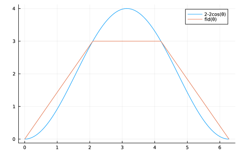
Figure 1: Fidelity as a function of the relative angle $\theta\in[0,2\pi)$ compared with the function $2-2\cos(\theta)$.

In the definition of fidelity we assumed $(\alpha,\beta)$ is uniformly distributed. However, the distribution of eigenvalues $(\alpha_{r},\beta_{s})$ may not be uniform. To understand the distribution of pairs of eigenvalues we need the definition of relative distribution.

Relative distribution.

In Definition 1.9 we defined $\Delta_{A,B}$, the relative distribution of $(A,B)$, as the distribution of the angle $\theta$ in the random process

1. Sample $(X,Y)$ from $D_{A,B}$.

2. Sample a pair of eigenvalues $(\alpha,\beta)$ of $X$ and $Y$ with probability $\langle P,Q\rangle$, where $P$ is the projection onto the $\alpha$-eigenspace of $X$ and $Q$ is the projection onto the $\beta$-eigenspace of $Y$.

3. Let $\theta\in[0,2\pi)$ be the relative angle between $\alpha$ and $\beta$, that is $\theta\coloneqq\measuredangle\alpha^{*}\beta$.

Fix a $\theta\in[0,2\pi)$ and a sample $(X,Y)\in D_{A,B}$ and let $X=\sum_{r}\alpha_{r}P_{r}$ and $Y=\sum_{s}\beta_{s}Q_{s}$ be the spectral decompositions. The relative weight of eigenspaces of $X$ and $Y$ on the angle $\theta$ is given by

$$w_{X,Y}(\theta)\coloneqq\sum_{\begin{subarray}{c}r,s:\\ \alpha_{r}^{*}\beta_{s}=\exp(i\theta)\end{subarray}}\langle P_{r},Q_{s}\rangle.$$

If there is no pair of eigenvalues $\alpha_{r}$ of $X$ and $\beta_{s}$ of $Y$ such that $\alpha_{r}^{*}\beta_{s}=\exp(i\theta)$, we let $w_{X,Y}(\theta)=0$. It should be intuitively clear (and this is made formal in Definition 6.2) that $\Delta_{A,B}(\theta)$ is the average of $w_{X,Y}(\theta)$ over all samples $(X,Y)\in D_{A,B}$. In Theorem 6.5, we showed that, in the limit of large dimension, the relative distribution $\Delta_{A,B}$ approaches the wrapped Cauchy distribution $\Delta_{\lambda}$ where $\lambda=\langle A,B\rangle$. This distribution $\Delta_{\lambda}$ is defined in the Preliminaries 3.2. Note that we can always increase the dimension of $A$ and $B$, by tensoring them with the identity operator, without changing the inner product $\langle A,B\rangle$ (and hence without changing the objective value of the solution in the CSP). Theorem 6.5 is therefore proving that $\Delta_{A\otimes I_{m},B\otimes I_{m}}\rightarrow\Delta_{\lambda}$ as $m\rightarrow\infty$. The plot of the wrapped Cauchy distribution $\Delta_{\lambda}$ for some real values of $\lambda=\langle A,B\rangle$ is given in Figure 2.

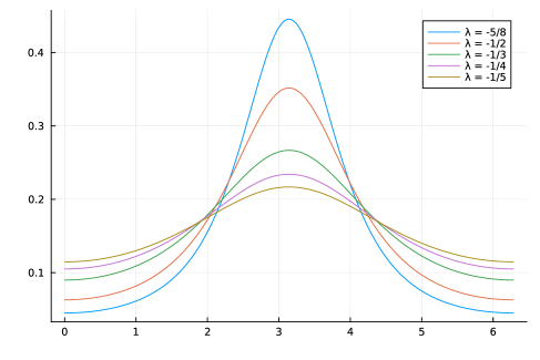
Figure 2: PDF of $\Delta_{\lambda}$ for some values of $\lambda$. The horizontal axis is the interval $[0,2\pi)$. The distributions are peaked at the angle $\measuredangle\lambda$ which for a negative real number $\lambda$ is always $\pi$.

It turns out that the expectation $\mathbb{E}[2-\langle\widetilde{X},\widetilde{Y}\rangle-\langle\widetilde{Y},\widetilde{X}\rangle]$ is a simple formula in terms of the fidelity function and relative distribution:

Lemma 2.2.

It holds that

$$\mathbb{E}[2-\langle\widetilde{X},\widetilde{Y}\rangle-\langle\widetilde{Y},\widetilde{X}\rangle] =\int_{\theta}\mathrm{fid}(\theta)d\Delta_{A,B}(\theta).$$

We prove a stronger version of this in Theorem 6.7. Since we can always increase the dimension of $A$ and $B$, in this integral formula we can replace $\Delta_{A,B}$ with the wrapped Cauchy distribution $\Delta_{\lambda}$. Now to prove (2.4) we just need to show that

$$\int_{\theta}\mathrm{fid}(\theta)d\Delta_{\lambda}(\theta)\geq 0.864(2-2\lambda),$$

for all $\lambda\in[-1/2,1]$. We prove this inequality by elementary means in Section 7 and Appendix B. This completes the sketch of the proof of Theorem 2.1.

2.2 Algebraic Approach

The strength of the analytic approach is its generality: it can be applied to any $2$-CSP where it successfully rounds any unitary solution to a nearby order-$k$ unitary solution. The drawback of the analytic approach is that, as in the example we just saw, the approximation ratio of $0.864$ is obtained only in the limit of large dimension. This is due to the fact that $\Delta_{A\otimes I_{m},B\otimes I_{m}}\rightarrow\Delta_{\lambda}$ only as $m\rightarrow\infty$.

We now present an outline of the algebraic approach that resolves this issue. Using this approach, we prove that an approximate solution of the same quality as the one in the analytic approach exists on a Hilbert space of dimension $2^{O(N)}$. The details of the algebraic approach are presented in Sections 8 and 9.

The key idea is to change the definition of Weyl-Brauer operators in the vector-to-unitary construction. The generalised Weyl-Brauer (GWB), as defined in Section 1.2.2, are a set of operators $\sigma_{1},\ldots,\sigma_{N}$ that are unitary matrices of order $3$, i.e. $\sigma_{i}^{*}\sigma_{i}=\sigma_{i}^{3}=1$ and they pairwise satisfy the relation $\sigma_{i}^{*}\sigma_{j}=-\sigma_{j}^{*}\sigma_{i}$ for all $i\neq j$. In Theorem 1.6 we prove that this set of operators exists on a Hilbert space of dimension $2^{O(N)}$. Similarly we can define order-$k$ generalised Weyl-Brauer operators denoted by $\mathrm{GWB}^{k}$ for any $k$.

Let $\vec{x}\mapsto U_{\vec{x}}$ be the vector-to-unitary construction using $\mathrm{GWB}^{k}$ operators. Then, as before, we can show that $U_{\vec{x}}$ is a unitary whenever $\vec{x}\in R^{N}$ is a unit vector. Additionally, in Section 5, we show that this generalised vector-to-unitary construction satisfies a strong isometry property, i.e. $\langle U_{\vec{x}}^{s},U_{\vec{y}}^{s}\rangle=\langle\vec{x},\vec{y}\rangle^{s}$ for all $0\leq s<k$ and all vectors $\vec{x},\vec{y}\in\mathbb{R}^{N}$.

Now consider the distribution $(U_{O\vec{x}},U_{O\vec{y}})$ where $O$ is a Haar random orthogonal matrix acting on $\mathbb{R}^{N}$. Note the similarity to the fixed inner product distribution $(VU_{\vec{x}},VU_{\vec{y}})$ where $V$ is Haar random unitary matrix acting on $\mathbb{C}^{2^{O(N)}}$. Notice also the following difference: the order of the randomness step and the vector-to-unitary step is switched. In particular in $(U_{O\vec{x}},U_{\vec{Oy}})$ we are using far less randomness. Despite this, using the strong isometry property, in Section 8 on algebraic relative distribution, we prove that the two distributions are the same as far as the relative distribution is concerned. This paves the path for the following algorithm.

In Section 9 we show that, for sufficiently large $k$, a slightly modified version of the following algorithm achieves an approximation ratio of $0.864$:

1 Solve the SDP relaxation to obtain vectors $\vec{x}_{1},\ldots,\vec{x}_{N}\in\mathbb{R}^{N}$.

2Sample an orthogonal matrix $O$ acting on $\mathbb{R}^{N}$ from the Haar measure.

3Apply the vector-to-unitary construction using $\mathrm{GWB}^{k}$ to obtain unitary operators $X_{i}=U_{O\vec{x}_{i}}$.

Round to the nearest order-$3$ unitary and return $\widetilde{X}_{1},\ldots,\widetilde{X}_{N}$.

Algorithm 2 Dimension-efficient approximation algorithm for $\mathrm{NC}\textit{-}\mathrm{Max}\textit{-}\mathrm{Lin}({3})$.

The dimension of the Hilbert space of the approximate solution is $2^{O(kN)}$ where $k$ is a sufficiently large constant.

Question 2.3.

Numerical evidence suggests that even for $k=3$, Algorithm 2 achieves the approximation ratio $0.864$. Can this be proven?

As mentioned above, the primary difference between Algorithm 1 and 2, is that the order of the randomness and vector-to-unitary steps is switched. In Algorithm 1, we first apply the vector-to-unitary construction (producing exponential-sized matrices), then sample a Haar random unitary acting on a Hilbert space of large dimension. In Algorithm 2, we first sample from the Haar measure on a Hilbert space of small dimension $N$, then apply the vector-to-unitary construction.

Question 2.4.

Can we reduce the amount of randomness needed in Algorithm 1? Could we switch Haar random unitaries with unitary designs? Could we derandomize it altogether?

Both algorithms apply the nonlinear operation $X\mapsto\widetilde{X}$ on matrices of exponential dimension in $N$. We need the spectral decomposition of $X$ to calculate $\widetilde{X}$. So it is natural to ask the following question about the vector-to-unitary construction.

Question 2.5.

Is there an efficient algorithm that given $\vec{x}$ and $t$ finds the $t$-th eigenvalue (in some ordering) of the operator $U_{\vec{x}}$?

Even though both algorithms give polynomial-sized descriptions for the approximate solutions, given that the solutions are exponential-sized, one cannot hope to even write down the matrices $\widetilde{X}_{1},\ldots,\widetilde{X}_{N}$. From the nonlocal games perspective, the output of the algorithm $\widetilde{X}_{1},\ldots,\widetilde{X}_{N}$ are observables of Alice and Bob in a quantum strategy with $O(N)$ qubits. Could the players be implemented efficiently on quantum computers?

Question 2.6.

Could the order-$3$ observable $\widetilde{U_{\vec{x}}}$ be implemented on a polynomial-sized quantum circuit?

3 Preliminaries

3.1 Notation

We use shorthand $[n]$ for the set $\{1,\ldots,n\}$. For $z\in\mathbb{C}$, we write $z^{\ast}$ for its complex conjugate, $\mathrm{Re}(z)$ for its real part, and $\measuredangle z$ for its argument, i.e. angle in the interval $[0,2\pi)$ such that $z=|z|e^{i\measuredangle z}$. Write $S^{1}\subseteq\mathbb{C}$ for the circle of radius $1$. We often represent $S^{1}$ by the interval $[0,2\pi)$. When doing so, we always assume addition is modulo $2\pi$.

The $k$-th roots of unity are $\{{e^{\frac{2\pi il}{k}}}|{l=0,\ldots,k-1}\}\subseteq S^{1}$ and a primitive $k$-th root of unity is a $k$-th root that is not an $l$-th root for any $l<k$; we write $\omega_{k}=e^{2\pi i/k}$, and drop the subscript when clear from the context. We let $\Omega_{k}$ denote $k$-simplex that is the convex hull of $k$th roots of unity.

We use vector notation $\vec{x}$ for elements of $\mathbb{R}^{d}$ or $\mathbb{C}^{d}$, and write the standard inner product $\langle\vec{x},\vec{y}\rangle=\sum_{i=1}^{d}x_{i}^{\ast}y_{i}$. We denote the Euclidean norm of a vector $\vec{x}$ as $\|\vec{x}\|=\sqrt{\langle\vec{x},\vec{x}\rangle}$.

We denote the set of $d\times d$ over a field $\mathbb{F}$ matrices by $\mathrm{M}_{d}(\mathbb{F})$. Write $1\in\mathrm{M}_{d}(\mathbb{F})$ for the identity element. Alternatively we write $I_{d}$ for the identity element when we want to be explicit about its dimension. More generally we denote the set of $d\times d^{\prime}$ matrices over a field $\mathbb{F}$ by $\mathrm{M}_{d\times d^{\prime}}(\mathbb{F})$. Sometimes we want to index entries of a matrix by finite sets that are not $[n]$; we write $\mathrm{M}_{E\times F}(\mathbb{F})$ for matrices in $\mathbb{F}$ with rows and columns indexed by sets $E$ and $F$, respectively. Important subsets of $\mathrm{M}_{d}(\mathbb{C})$ are the positive (semidefinite) matrices $\mathrm{M}_{d}(\mathbb{C})_{\geq 0}$ and the positive definite matrices $\mathrm{M}_{d}(\mathbb{C})_{>0}$; write $X\geq 0$ to mean $X\in\mathrm{M}_{d}(\mathbb{C})_{\geq 0}$ when the dimension of $X$ is evident. Write also $\mathrm{GL}_{d}(\mathbb{C})$ for the group of invertible matrices and $\mathrm{U}_{d}(\mathbb{C})$ for the subgroup of unitary matrices. As for complex numbers, we write $X^{\ast}$ for the adjoint (hermitian conjugate) of a matrix $X$. We write $\operatorname{tr}:\mathrm{M}_{d}(\mathbb{C})\rightarrow\mathbb{C}$ for the normalised trace $\operatorname{tr}(X)=\frac{1}{d}\sum_{i=1}^{d}X_{ii}$; this gives rise to the Hilbert-Schmidt inner product $\langle X,Y\rangle=\operatorname{tr}(X^{\ast}Y)$. We make use of the operator norm $\|X\|_{\mathrm{op}}=\sup\big{\{}{\|Xv\|}\big{|}{\|v\|\leq 1}\big{\}}$ and the little Frobenius norm $\|X\|=\sqrt{\langle X,X\rangle}$.

For a Hilbert space $\mathcal{H}$, we denote the set of bounded linear operators on $\mathcal{H}$ as $\mathrm{B}(\mathcal{H})$. These are exactly the linear operators that are continuous with respect to the norm topology on $\mathcal{H}$. If $\mathcal{H}$ is finite-dimensional, then $\mathrm{B}(\mathcal{H})\cong\mathrm{M}_{d}(\mathbb{C})$ for $d=\dim\mathcal{H}$; we often make no distinction between these.

3.2 Probability Theory

A measurable space is a pair $(\Omega,\mathscr{S})$ where the set $\Omega$ is called the sample space and $\mathscr{S}$, a $\sigma$-algebra on $\Omega$, is called the event space. For a topological space $\Omega$, there is a canonical choice of $\sigma$-algebra to give it a measurable structure, the Borel algebra $\mathscr{B}(\Omega)$. See [84] for a reference on measure theory.

A probability space is $(\Omega,\mathscr{S},\mathcal{D})$ where $\mathcal{D}$ is a measure on $(\Omega,\mathscr{S})$ such that $\mathcal{D}(\Omega)=1$. We call $\mathcal{D}$ a distribution on $\Omega$.

Given another measurable space $(M,\mathscr{F})$, a random variable on $(\Omega,\mathscr{S},\mathcal{D})$ is a measurable function $X:\Omega\rightarrow M$, i.e. a function for which $X^{-1}(E)\in\mathscr{S}$ for all $E\in\mathscr{F}$. This induces a distribution on $M$ where $\mu_{X}(E)\coloneqq\mathcal{D}(X^{-1}(E))$ for all $E\in\mathscr{F}$; this is called the distribution of $X$. We also use probability notation for this distribution, writing $\Pr\left[X\in E\right]\coloneqq\mu_{X}(E)$. Two random variables $X,Y$ are independent if for all measurable $E,F$ we have $\Pr\left[X\in E\land Y\in F\right]=\Pr\left[X\in E\right]\Pr\left[Y\in F\right]$.

If $M$ is in fact a measure space with its own measure $\nu$ — for example if $M$ is a finite-dimensional real vector space with the Lebesgue measure $\Lambda$ — then we can compare this to the measure $\mu_{X}$. If $\mu_{X}$ is absolutely continuous with respect to $\nu$ (for all $E\in\mathscr{F}$, $\nu(E)=0$ implies $\mu_{X}(E)=0$), then we can define the Radon-Nikodym derivative of $\mu_{X}$ with respect to $\nu$, which we refer to as the probability density function (PDF) $p_{X}=\frac{d\mu_{X}}{d\nu}:M\rightarrow\mathbb{R}_{\geq 0}$. Another way to state this relationship is $\mu_{X}(E)=\int_{E}p_{X}(x)d\nu(x)$. More generally, we can also consider the PDF of any distribution $\mathcal{D}$ on $M$ as the Radon-Nikodym derivative $p_{\mathcal{D}}=\frac{d\mathcal{D}}{d\nu}$, assuming $\mathcal{D}$ is absolutely continuous with respect to $\nu$.

If $M$ is a real or complex vector space, the expectation of $X$ is given by the integral $\mathbb{E}X=\int_{\Omega}X(\omega)d\mu(\omega)=\int_{M}xd\mu_{X}(x)$. Also, for a function $f:M\rightarrow\mathbb{C}$, the composition $f\circ X$ is also a random variable, so we can always write $\mathbb{E}_{X}f\circ X=\mathbb{E}f\circ X=\int_{\Omega}f(X(\omega))d\mu(\omega)$. We write simply $f(X)$ when referring to $f\circ X$.

Definition 3.1.

A sequence of random variables $(X_{n})$ converges in distribution to a random variable $X$ if for all measurable $E\subseteq M$,

$$\lim_{n\rightarrow\infty}\Pr\left[X_{n}\in E\right]=\Pr\left[X\in E\right].$$

If $\mathscr{F}=\mathscr{B}(M)$, this is equivalent to $\mathbb{E}f(X_{n})\rightarrow\mathbb{E}f(X)$ for all bounded continuous functions $f:M\rightarrow\mathbb{R}$.

It is not necessary to make reference to an underlying sample space to define and work with a random variable, so we generally avoid it. Instead, we define random variables according to a distribution. For a distribution $\mathcal{D}$ (probability measure) on a measurable space $M$, we say a random variable $X:\Omega\rightarrow M$ is distributed according to $\mathcal{D}$ if $\mu_{X}=\mathcal{D}$. We denote this $X\sim\mathcal{D}$. Below, we present the standard distributions we use.

• Dirac Delta Distribution: For any measurable space $(M,\mathscr{F})$ and $m\in M$, this is the distribution

  $$\delta_{m}(E)=\begin{cases}1&\quad m\in E,\\ 0&\quad\text{otherwise}.\end{cases}$$ (3.1)

• Complex Normal Distribution: $\mathcal{CN}(m,\sigma)$ for mean $m\in\mathbb{C}$ and standard deviation $\sigma>0$ is the distribution on $\mathbb{C}$ with PDF

  $$p_{\mathcal{CN}(m,\sigma)}(z)=\frac{1}{2\pi\sigma^{2}}e^{-\frac{|z-m|^{2}}{2\sigma^{2}}},$$ (3.2)

  with respect to the Lebesgue measure on $\mathbb{C}$. We call $\mathcal{CN}=\mathcal{CN}(0,1)$ the standard complex normal distribution.

• Vector Complex Normal Distribution: $\mathcal{CN}(d,\vec{m},\Sigma)$ for dimension $d\in\mathbb{N}$, mean $\vec{m}\in\mathbb{C}^{d}$, and covariance matrix $\Sigma\in\mathrm{M}_{d}(\mathbb{C})_{>0}$ is the distribution on $\mathbb{C}^{d}$ with PDF

  $$p_{\mathcal{CN}(d,\vec{m},\Sigma)}(\vec{z})=\frac{1}{(2\pi\det\Sigma)^{d}}e^{-\frac{1}{2}\langle\vec{z}-\vec{m},\Sigma^{-1}(\vec{z}-\vec{m})\rangle},$$ (3.3)

  with respect to the Lebesgue measure on $\mathbb{C}^{d}$. We call $\mathcal{CN}(d)=\mathcal{CN}(d,\vec{0},1)$ the standard vector complex normal distribution. Note that if $\Sigma$ is diagonal, then the components of a random variable $\vec{Z}\sim\mathcal{CN}(d,\vec{m},\Sigma)$ are independent.

• Wrapped Cauchy Distribution: $\mathcal{W}(\theta_{0},\gamma)$ for peak position $\theta_{0}\in[0,2\pi)$ and scale factor $\gamma>0$ is the distribution on $[0,2\pi)\cong S^{1}$ with PDF

  $$p_{\mathcal{W}(\theta_{0},\gamma)}(\theta)=\frac{\sinh(\gamma)}{2\pi(\cosh(\gamma)-\cos(\theta-\theta_{0}))},$$ (3.4)

  with respect to the Lebesgue measure on $[0,2\pi)$. For $\lambda\in\mathbb{C}$ with $|\lambda|\leq 1$ we define the distribution $\Delta_{\lambda}\coloneqq\mathcal{W}(\measuredangle\lambda,-\ln|\lambda|)$ when $|\lambda|<1$ and $\Delta_{\lambda}\coloneqq\delta_{\measuredangle\lambda}$ when $|\lambda|=1$.

• Haar Distribution: For any compact topological group $G$, there exists a unique distribution $\mathrm{Haar}(G)$ on $(G,\mathscr{B}(G))$ such that for all $E\subseteq G$ Borel-measurable and $g\in G$,

  $$\mathrm{Haar}(G)(E)=\mathrm{Haar}(G)(gE)=\mathrm{Haar}(G)(Eg).$$

  We make use of $\mathrm{Haar}(\mathrm{U}_{d}(\mathbb{C}))$.

We will be largely interested in random variables $X$ on the circle $[0,2\pi)\cong\mathbb{R}/2\pi\mathbb{Z}\cong S^{1}$. Here, we take the characteristic function of $X$ to be the Fourier series

$$\chi_{X}:\mathbb{Z}\rightarrow\mathbb{C},\quad\chi_{X}(n)=\mathbb{E}(e^{inX}).$$

If $\mu_{X}$ is absolutely continuous, then we have $\chi_{X}=\widehat{p}_{X}$, the Fourier series of the PDF. The Fourier series of an integrable function $f:[0,2\pi)\rightarrow\mathbb{C}$ is the function $\widehat{f}:\mathbb{Z}\rightarrow\mathbb{C}$ defined as

$$\widehat{f}(n)=\int_{0}^{2\pi}f(\theta)e^{in\theta}d\theta.$$

The characteristic function can similarly be defined for distributions. For example the characteristic function of the Dirac delta distribution $\delta_{\theta_{0}}$ on $[0,2\pi)$ is

$$\chi_{\delta_{\theta_{0}}}(n)=e^{in\theta_{0}};$$

and the characteristic function of the wrapped Cauchy distribution $\mathcal{W}(\theta_{0},\gamma)$ is

$$\chi_{\mathcal{W}(\theta_{0},\gamma)}(n)=e^{-|n|\gamma+in\theta_{0}}.$$

This implies that $\chi_{\Delta_{\lambda}}(n)=\lambda^{n}$ for $n\geq 0$ and $\chi_{\Delta_{\lambda}}(n)=(\lambda^{\ast})^{-n}$ for $n<0$.

Theorem 3.2 (Parseval).

Let $f,g:[0,2\pi)\rightarrow\mathbb{C}$ be square-integrable functions on the circle ($f,g\in L^{2}[0,2\pi)$). Then

$$\int_{0}^{2\pi}f(\theta)^{\ast}g(\theta)d\theta=\frac{1}{2\pi}\sum_{n\in\mathbb{Z}}\widehat{f}(n)^{\ast}\widehat{g}(n).$$ (3.5)

In particular, the series $\frac{1}{2\pi}\sum_{n\in\mathbb{Z}}\widehat{f}(n)^{\ast}\widehat{g}(n)$ converges.

This theorem states that the operation of taking the Fourier series is an isometry $L^{2}[0,2\pi)\rightarrow\ell^{2}\mathbb{Z}$ with the correct normalisation on the inner products. Using Parseval, when $X$ is a random variable on $[0,2\pi)$ with square-integrable PDF and $f:[0,2\pi)\rightarrow\mathbb{C}$ is a square-integrable function, we have

$$\int_{0}^{2\pi}f(\theta)d\mu_{X}(\theta)=\frac{1}{2\pi}\sum_{n\in\mathbb{Z}}\widehat{f}(-n)\chi_{X}(n).$$ (3.6)

Theorem 3.3 (Lévy’s continuity theorem on the circle).

A sequence of random variables $(X_{n})$ on the $[0,2\pi)$ converges in distribution if and only if the sequence of characteristic functions $(\chi_{X_{n}})$ converges pointwise.

The above theorem is a consequence of the Stone-Weierstrass theorem.

3.3 Free Probability

We will also make use of results from free probability theory. This is the study of noncommutative random variables and our main reference for this section is [85].

A noncommutative probability space is a unital algebra $\mathcal{A}$ equipped with a linear functional $\tau:\mathcal{A}\rightarrow\mathbb{C}$ such that $\tau(1)=1$, called the expectation. We will always assume, as is commonly done, that $\mathcal{A}$ is a $C^{\ast}$-algebra, i.e. $\mathcal{A}$ has a conjugate-linear involution $\ast$ and is complete with respect to a submultiplicative norm satisfying $\|a^{\ast}a\|=\|a\|^{2}$; and that $\tau$ is a faithful tracial state, i.e. that $\tau(a^{\ast}a)\geq 0$, if $\tau(a^{\ast}a)=0$ then $a=0$, and $\tau(ab)=\tau(ba)$. Elements of a noncommutative probability space are called noncommutative random variables. As a first example, it is worth noting that commutative probability theory, as seen in the previous section, fits as a special case of noncommutative probability theory. In fact, given a probability space $(\Omega,\mathscr{S},\mathcal{D})$, its set of (bounded, complex-valued) random variables corresponds to the noncommutative probability space $\mathcal{A}=L^{\infty}(\Omega,\mathcal{D})$ with $\tau(X)=\int X(\omega)d\mathcal{D}(\omega)=\mathbb{E}X$. Another example of noncommutative probability space is $(\mathrm{M}_{d}(\mathbb{C}),\operatorname{tr})$.

A mixed $\ast$-moment of a collection of noncommutative random variables $a_{1},\ldots,a_{n}\in\mathcal{A}$ is an expectation of the form $\tau(a_{i_{1}}^{e_{1}}\cdots a_{i_{m}}^{e_{m}})$, where $i_{j}\in[n]$ and $e_{j}\in\{1,\ast\}$. For a single element $a\in\mathcal{A}$, the $\ast$-moments of $a$ are the mixed $\ast$-moments of $a$. For normal $a\in\mathcal{A}$, i.e. $aa^{\ast}=a^{\ast}a$, the $\ast$-moments are simply $\tau((a^{\ast})^{k}a^{l})$ for integers $k,l\geq 0$. In this case, the idea of a probability distribution for random variables generalises quite directly. There exists a unique measure $\mu_{a}$ on (some compact subset of) $\mathbb{C}$ such that all the $\ast$-moments can be written as

$$\tau((a^{\ast})^{k}a^{l})=\int(z^{\ast})^{k}z^{l}d\mu_{a}(z).$$

Knowing the $\ast$-moments, the expectation of any element of $C^{\ast}\!\!\vphantom{a}\left\langle\smash{a}\right\rangle$, the unital subalgebra generated by $a$, can be computed.

The $\ast$-algebra of univariate $\ast$-polynomials, denoted $\mathbb{C}^{\ast}\!\!\vphantom{x}\left\langle\smash{x}\right\rangle$, is the $\ast$-algebra generated by the free variable $x$. This extends to multivariate $\ast$-polynomials $\mathbb{C}^{\ast}\!\!\vphantom{x_{1},\ldots,x_{n}}\left\langle\smash{x_{1},\ldots,x_{n}}\right\rangle$.

Definition 3.4.

A set of noncommutative random variables $a_{1},\ldots,a_{n}\in\mathcal{A}$ is freely independent (or free for short) if, for any $i_{1},\ldots,i_{m}\in[n]$ such that $i_{j}\neq i_{j+1}$ and $\ast$-polynomials $P_{1},\ldots,P_{m}\in\mathbb{C}^{\ast}\!\!\vphantom{x}\left\langle\smash{x}\right\rangle$ such that $\tau(P_{j}(a_{i_{j}}))=0$, we have that

$$\tau(P_{1}(a_{i_{1}})\cdots P_{m}(a_{i_{m}}))=0.$$

The usual commutative notion of independence guarantees the above property only in the case where all the $i_{j}$ are distinct, which can be supposed due to commutativity. If the $\ast$-moments of a set of free random variables are known, then any of the mixed $\ast$-moments can be computed.

Definition 3.5.

A collection of sequences $(a_{1,n}),\ldots,(a_{l,n})$ of noncommutative random variables such that $a_{i,n}\in(\mathcal{A}_{n},\tau_{n})$ converges in $\ast$-distribution to a collection of noncommutative random variables $a_{1},\ldots,a_{l}\in(\mathcal{A},\tau)$ if all the mixed $\ast$-moments converge, i.e.

$$\lim_{n\rightarrow\infty}\tau_{n}(a_{i_{1},n}^{e_{1}}\cdots a_{i_{m},n}^{e_{m}})=\tau(a_{i_{1}}^{e_{1}}\cdots a_{i_{m}}^{e_{m}}).$$

We write this as $a_{1,n},\ldots,a_{l,n}\rightarrow a_{1},\ldots,a_{l}$ ($\ast$-dist).

The idea of a Haar-random unitary generalises naturally to the context of free probability. We say a noncommutative random variable $u\in\mathcal{A}$ is a Haar unitary if $u$ is unitary ($u^{\ast}u=uu^{\ast}=1$) and the $\ast$-moments $\tau(u^{k})=\delta_{k,0}$ for all $k\in\mathbb{Z}$. This generalises the Haar distribution on the unitary group as a Haar-random unitary $U$ on $\mathrm{U}_{d}(\mathbb{C})$ satisfies $\int\operatorname{tr}(U^{k})dU=\delta_{k,0}$. A Haar-random unitary can be seen as a noncommutative random variable on the space $\mathcal{A}=\mathrm{M}_{d}(L^{\infty}(\Omega,\mathcal{D}))$ for some probability space $(\Omega,\mathscr{S},\mathcal{D})$. This space has natural expectation $\tau(a)=\int\operatorname{tr}(a(\omega))d\mathcal{D}(\omega)$.

We make use of the following theorem.

Theorem 3.6 (23.13 in [85]).

Let $(d_{n})$ be a sequence of natural numbers such that $d_{n}\rightarrow\infty$. Let $(U_{n})$ be a sequence of random variables such that $U_{n}\sim\mathrm{Haar}(\mathrm{U}_{d_{n}}(\mathbb{C}))$, and let $(A_{n})$ be a sequence of matrices such that $A_{n}\in\mathrm{M}_{d_{n}}(\mathbb{C})$. Suppose that the limiting $\ast$-moments $\lim_{n\rightarrow\infty}\operatorname{tr}(A_{n}^{e_{1}}\cdots A_{n}^{e_{m}})$ for $e_{i}\in\{1,\ast\}$ all exist. Then, there exists a noncommutative probability space $\mathcal{A}$ and freely independent random variables $u,a\in\mathcal{A}$ such that $U_{n},A_{n}\rightarrow u,a$ ($\ast$-dist).

Note that, by the convergence in $\ast$-distribution, we have in particular that $u$ is Haar unitary and the $\ast$-moments of $a$ are the limiting $\ast$-moments of $A_{n}$. In this context, we say that $(U_{n})$ and $(A_{n})$ are asymptotically free.

3.4 Group Theory

For any group $G$ and subset $A\subseteq G$, we write $\vphantom{A}\left\langle\smash{A}\right\rangle$ for the subgroup generated by $A$, and $\llangle A\rrangle$ for its normal closure. The identity element of a group is denoted $e$. For two group elements $g,h$ we let $[g,h]$ denote the commutator $ghg^{-1}h^{-1}$.

Presentations. We present groups we work with by means of generators and relations. A set of generators is a set of symbols $S$, and a set of relators is a set $R$ of words in $S\cup S^{-1}$, where $S^{-1}=\left\{{x^{-1}}\middle|{x\in S}\right\}$. Each relator $r\in R$ corresponds to the relation $r=e$. The free group generated by $S$, $\langle S\rangle$ is the group of words in $S\cup S^{-1}$ under concatenation — the identity element is the empty word $e$ and inverses exist since we include $S^{-1}$ in the generating set. Then, the group generated by generators $S$ and relators $R$ is the quotient group $\vphantom{SR}\left\langle\smash{S}:\smash{R}\right\rangle:=\langle S\rangle/\langle\!\langle R\rangle\!\rangle$. As noted, we can equivalently phrase the relators a relations on the words in $S$. A group $G$ is finitely-presented if $G=\vphantom{SR}\left\langle\smash{S}:\smash{R}\right\rangle$ where $S$ and $R$ are both finite sets.

Free and amalgamated products. Given two groups $G$ and $H$, their free product is the group $G\ast H$ generated by $G\cup H$ with no relations between the elements of $G$ and $H$ except that the identities $e_{G}=e_{H}$. The elements of $G\ast H$ are words in $G\cup H$. Given subgroups $A\leq G$ and $B\leq H$ that are isomorphic, the amalgamated product $G\ast_{A}H$ is the quotient $(G\ast H)/\langle\!\langle R\rangle\!\rangle$ where $R$ is the set of relators $a^{-1}\phi(a)$ for $a\in A$, where $\phi:A\rightarrow B$ is the isomorphism.

Representations. A ($\mathbb{C}$-linear) representation of a group $G$ is a homomorphism $\varrho:G\rightarrow\mathrm{GL}_{d}(\mathbb{C})$. Suppose $G$ is a finite group. Then, $\varrho$ is equivalent to a unitary representation $\varrho(G)\in\mathrm{U}_{d}(\mathbb{C})$ by conjugation, so we may assume any representation is unitary. Also, $\varrho$ decomposes as a direct sum of irreducibles (representations with no nontrivial invariant subspaces). Every finite group has finitely many classes of irreducible representations, modulo equivalence by conjugation. For conciseness, we refer to these classes as irreps. The number of these irreps is equal to the number of conjugacy classes, subsets $\mathrm{Cl}(g)=\left\{{hgh^{-1}}\middle|{G}\right\}$ that partition $G$. See [86] for a full treatment.

Group algebras. For any group $G$, the group algebra $\mathbb{C}[G]$ is the set of finitely-supported functions $G\rightarrow\mathbb{C}$. We write an element $x\in\mathbb{C}[G]$ as $x=\sum_{g\in G}x(g)g$. $\mathbb{C}[G]$ is an algebra as it has a natural structure as a $\mathbb{C}$-vector space, and it also has a product given by convolution: $xy=\sum_{g,h\in G}x(g)y(h)gh=\sum_{g\in G}\sum_{h\in G}x(gh^{-1})y(h)g$. The multiplicative identity in $\mathbb{C}[G]$ is the group identity $e$. Further, $\mathbb{C}[G]$ is a $\ast$-algebra with involution $x^{\ast}=\sum_{g}x(g)^{\ast}g^{-1}$. The $\ast$-homomorphisms $\mathbb{C}[G]\rightarrow\mathrm{B}(\mathcal{H})$ correspond exactly to the unitary representations of $G$.

3.5 Von Neumann Algebras

A von Neumann algebra is a unital $\ast$-subalgebra $\mathcal{M}\subseteq\mathrm{B}(\mathcal{H})$ for some Hilbert space $\mathcal{H}$ that is equal to its double commutant $\mathcal{M}=\mathcal{M}^{\prime\prime}$, where $S^{\prime}:=\left\{{x\in\mathrm{B}(\mathcal{H})}\middle|{xy=yx\;\forall\,y\in S}\right\}$ for any $S\subseteq\mathrm{B}(\mathcal{H})$. The double commutant condition is equivalent to having $\mathcal{M}$ be closed in the strong, weak, or weak-$\ast$ operator topologies on $\mathrm{B}(\mathcal{H})$. In particular, the weak-$\ast$ topology is the smallest topology making any bounded linear functional continuous. A sequence $(x_{n})$ converges to $x$ in the weak-$\ast$ topology if, for any bounded linear functional $\phi:\mathrm{B}(\mathcal{H})\rightarrow\mathbb{C}$, the sequence $\phi(x_{n})\rightarrow\phi(x)$ in $\mathbb{C}$.

We focus mainly on finite von Neumann algebras: $\mathcal{M}$ is finite iff it has a weak-$\ast$ continuous tracial state $\tau:\mathcal{M}\rightarrow\mathbb{C}$, that is a faithful positive linear functional such that $\tau(xy)=\tau(yx)$. A functional $\tau$ is weak-$\ast$ continuous if for any weak-$\ast$ convergent sequence $(x_{n})\rightarrow x$, then $\tau(x_{n})\rightarrow\tau(x)$. An important fact about finite von Neumann algebras is that any compression remains finite. That is, for any nonzero projection $p\in\mathcal{M}$, i.e. $p=p^{\ast}=p^{2}$, $p\mathcal{M}p\subseteq\mathrm{B}(p\mathcal{H})$ is a von Neumann algebra with trace $\frac{1}{\tau(p)}\tau|_{p\mathcal{M}p}$, so it is finite. Note that if $p$ is also central, then $p\mathcal{M}p=p\mathcal{M}$.

The most important examples of von Neumann algebras we use are von Neumann group algebras. Let $G$ be an (infinite discrete) group, and consider the evaluation map $\tau:\mathbb{C}[G]\rightarrow\mathbb{C}$, $x\mapsto x(e)$. $\tau$ is a unital linear functional, and it is positive and faithful as

$$\tau(x^{\ast}x)=\sum_{g,h}x(g)^{\ast}x(h)\tau(g^{-1}h)=\sum_{g}|x(g)|^{2},$$

which is positive, and $0$ if and only if all the terms are $0$. Also, $\tau$ is tracial as

$$\tau(xy)=\sum_{g}x(g)y(g^{-1})=\sum_{g}y(g)x(g^{-1})=\tau(yx).$$

We call this the canonical trace on $\mathbb{C}[G]$. Further, $\langle x,y\rangle:=\tau(x^{\ast}y)$ gives an inner product on $\mathbb{C}[G]$. Consider the completion of $\mathbb{C}[G]$ with respect to the topology generated by the inner product, denoted $\ell^{2}G$. This is a Hilbert space. $\mathbb{C}[G]$ acts by left multiplication on $\ell^{2}G$, therefore $\mathbb{C}[G]$ embeds into $\mathrm{B}(\ell^{2}G)$. We define the von Neumann group algebra $\mathrm{L}(G)$ by the double commutant of the image of $\mathbb{C}[G]$ in $\mathrm{B}(\ell^{2}G)$. $\mathrm{L}(G)$ is a finite von Neumann algebra since the canonical trace $\tau$ of $\mathbb{C}[G]$ extends to a weak-$\ast$ continuous trace on $\mathrm{L}(G)$. For finite $G$ we have $\ell^{2}G=\mathbb{C}[G]=\mathrm{L}(G)$ as every finite vector space is complete.

For a complete introduction to von Neumann algebras, see [87]

3.6 Semidefinite Programming

A semidefinite program (SDP) is any optimization problem of the form:

    maximize: $$\langle C,X\rangle$$ (3.7)

subject to: $$\mathcal{A}_{i}(X)=B_{i}\text{ for }i\in\{1,\ldots,m\}$$

$$X\in\mathrm{M}_{d}(\mathbb{C})_{\geq 0},$$

where $C\in\mathrm{M}_{d}(\mathbb{C}),B_{i}\in\mathrm{M}_{d_{i}}(\mathbb{C})$ are Hermitian and $\mathcal{A}_{i}:\mathrm{M}_{d}(\mathbb{C})\to\mathrm{M}_{d_{i}}(\mathbb{C})$ are linear maps. Since any feasible solution $X$ is positive semidefinite, we can use its Gram matrix characterisation to equivalently write the SDP in a vector form. Gram vectors are $\vec{v}_{i}\in\mathbb{C}^{d}$ such that $X_{ij}=\langle\vec{v}_{i},\vec{v}_{j}\rangle$. SDPs can be approximated to any precision $\varepsilon$ in time $\mathrm{poly}(d,\log(1/\varepsilon))$ [88]. For more on SDPs, see [89, 90].

4 CSP Definitions

In this section, we gather all the different variations of CSPs we defined. In Section 4.1, we give the expressions of classical and noncommutative variants of $\mathrm{Max}\textit{-}\mathrm{Lin}({k})$. In Sections 4.2 and 4.3, we define homogeneous and smooth CSPs, respectively.

4.1 General Definitions

The $\mathrm{Max}\textit{-}\mathrm{Lin}({k})$ is the problem

maximize: $$\sum_{(i,j)\in\mathcal{E}}\frac{w_{ij}}{k}{\sum_{s=0}^{k-1}\omega^{-c_{ij}s}x_{i}^{-s}x_{j}^{s}}+\sum_{(i,j)\in\mathcal{I}}w_{ij}\big{(}1-\frac{1}{k}{\sum_{s=0}^{k-1}\omega^{-c_{ij}s}x_{i}^{-s}x_{j}^{s}}\big{)}$$ (4.1)

subject to: $$x_{i}^{k}=1\text{ and }x_{i}\in\mathbb{C},$$

where it is always understood that $c_{ij}=-c_{ji}$ and $w_{ij}=w_{ji}\geq 0$ and $\mathcal{E}$ denotes the set of equation constraints $x_{i}^{-1}x_{j}=\omega^{c_{ij}}$ and $\mathcal{I}$ denotes the set of inequation constraints $x_{i}^{-1}x_{j}\neq\omega^{c_{ij}}$. We always let $N$ denote the number of variables in the instance.

The norm $\mathrm{Max}\textit{-}\mathrm{Lin}({k})$ is

maximize: $$\Big{\|}\sum_{(i,j)\in\mathcal{E}}\frac{w_{ij}}{k}{\sum_{s=0}^{k-1}\omega^{-c_{ij}s}X_{i}^{-s}X_{j}^{s}}+\sum_{(i,j)\in\mathcal{I}}w_{ij}\big{(}1-\frac{1}{k}{\sum_{s=0}^{k-1}\omega^{-c_{ij}s}X_{i}^{-s}X_{j}^{s}}\big{)}\Big{\|}_{\mathrm{op}}$$ (4.2)

subject to: $$X_{i}^{*}X_{i}=X_{i}^{k}=1,$$

which can also be written equivalently in the form

maximize: $$\langle\mspace{0.5mu}\phi\mspace{0.5mu}\rvert\Big{\lparen}\sum_{(i,j)\in\mathcal{E}}\frac{w_{ij}}{k}{\sum_{s=0}^{k-1}\omega^{-c_{ij}s}X_{i}^{-s}X_{j}^{s}}+\sum_{(i,j)\in\mathcal{I}}w_{ij}\big{(}1-\frac{1}{k}{\sum_{s=0}^{k-1}\omega^{-c_{ij}s}X_{i}^{-s}X_{j}^{s}}\big{)}\Big{\rparen}\lvert\mspace{0.5mu}\phi\mspace{0.5mu}\rangle$$ (4.3)

subject to: $$\vphantom{\phi}\left\langle\smash{\phi}\middle|\smash{\phi}\right\rangle=1,$$

$$X_{i}^{*}X_{i}=X_{i}^{k}=1.$$

Although not immediately obvious, this problem is equivalent to an SDP. So in addition to norm $\mathrm{Max}\textit{-}\mathrm{Lin}({k})$, we sometimes refer to it as the canonical SDP relaxation of $\mathrm{Max}\textit{-}\mathrm{Lin}({k})$ (as well as $\mathrm{NC}\textit{-}\mathrm{Max}\textit{-}\mathrm{Lin}({k})$). The canonical SDP relaxation of the special case of homogeneous $\mathrm{Max}\textit{-}\mathrm{Lin}({k})$ is different and is defined in the next section.

The noncommutative $\mathrm{Max}\textit{-}\mathrm{Lin}({k})$ (which we also sometimes referred to as tracial $\mathrm{Max}\textit{-}\mathrm{Lin}({k})$), denoted by $\mathrm{NC}\textit{-}\mathrm{Max}\textit{-}\mathrm{Lin}({k})$, is

maximize: $$\operatorname{tr}\Big{(}\sum_{(i,j)\in\mathcal{E}}\frac{w_{ij}}{k}{\sum_{s=0}^{k-1}\omega^{-c_{ij}s}X_{i}^{-s}X_{j}^{s}}+\sum_{(i,j)\in\mathcal{I}}w_{ij}\big{(}1-\frac{1}{k}{\sum_{s=0}^{k-1}\omega^{-c_{ij}s}X_{i}^{-s}X_{j}^{s}}\big{)}\Big{)}$$ (4.4)

subject to: $$X_{i}^{*}X_{i}=X_{i}^{k}=1.$$

We can equivalently write this using inner products

maximize: $$\sum_{(i,j)\in\mathcal{E}}\frac{w_{ij}}{k}{\sum_{s=0}^{k-1}\omega^{-c_{ij}s}\langle X_{i}^{s},X_{j}^{s}\rangle}+\sum_{(i,j)\in\mathcal{I}}w_{ij}\big{(}1-\frac{1}{k}{\sum_{s=0}^{k-1}\omega^{-c_{ij}s}\langle X_{i}^{s},X_{j}^{s}\rangle}\big{)}$$ (4.5)

subject to: $$X_{i}^{*}X_{i}=X_{i}^{k}=1.$$

The unitary relaxations are obtained when dropping the condition $X_{i}^{k}=1$ from these CSPs. In all the noncommutative problems it is always assumed that the optimization is over all finite-dimensional Hilbert spaces.

4.2 Homogeneous CSPs

Homogeneous $\mathrm{Max}\textit{-}\mathrm{Lin}({k})$, denoted by $\mathrm{HMax}\textit{-}\mathrm{Lin}({k})$, is

maximize: $$\sum_{(i,j)\in\mathcal{E}}\frac{w_{ij}}{k}{\sum_{s=0}^{k-1}x_{i}^{-s}x_{j}^{s}}+\sum_{(i,j)\in\mathcal{I}}w_{ij}\Big{\lparen}1-\frac{1}{k}{\sum_{s=0}^{k-1}x_{i}^{-s}x_{j}^{s}}\Big{\rparen}$$ (4.6)

subject to: $$x_{i}^{k}=1\text{ and }x_{i}\in\mathbb{C}.$$

The noncommutative $\mathrm{HMax}\textit{-}\mathrm{Lin}({k})$, denoted by $\mathrm{NC}\textit{-}\mathrm{HMax}\textit{-}\mathrm{Lin}({k})$, is

maximize: $$\sum_{(i,j)\in\mathcal{E}}\frac{w_{ij}}{k}{\sum_{s=0}^{k-1}\langle X_{i}^{s},X_{j}^{s}\rangle}+\sum_{(i,j)\in\mathcal{I}}w_{ij}\Big{\lparen}1-\frac{1}{k}{\sum_{s=0}^{k-1}\langle X_{i}^{s},X_{j}^{s}\rangle}\Big{\rparen}$$ (4.7)

subject to: $$X_{i}^{*}X_{i}=X_{i}^{k}=1.$$

By the canonical SDP relaxation of both these problems we mean

maximize: $$\sum_{(i,j)\in\mathcal{E}}\frac{w_{ij}}{k}(1+(k-1)X_{ij})+\sum_{(i,j)\in\mathcal{I}}w_{ij}\frac{k-1}{k}(1-X_{ij})$$ (4.8)

subject to: $$X\in\mathrm{M}_{N}(\mathbb{R})_{\geq 0},$$

$$X_{ii}=1,$$

$$X_{ij}\geq-\frac{1}{k-1},$$

which can be equivalently written in the vector form as

maximize: $$\sum_{(i,j)\in\mathcal{E}}\frac{w_{ij}}{k}(1+(k-1)\langle\vec{x}_{i},\vec{x}_{j}\rangle)+\sum_{(i,j)\in\mathcal{I}}w_{ij}\frac{k-1}{k}(1-\langle\vec{x}_{i},\vec{x}_{j}\rangle)$$ (4.9)

subject to: $$\vec{x}_{i}\in\mathbb{R}^{N},$$

$$\|\vec{x}_{i}\|=1,$$

$$\langle\vec{x}_{i},\vec{x}_{j}\rangle\geq-\frac{1}{k-1}.$$

To see that this is indeed a relaxation, suppose $X_{1},\ldots,X_{n}$ is any feasible solution to $\mathrm{NC}\textit{-}\mathrm{HMax}\textit{-}\mathrm{Lin}({k})$. We construct a feasible solution $X$ in the SDP achieving the same objective value as $X_{1},\ldots,X_{n}$. For $0\leq s<k$ let $W_{s}$ be the matrix defined so that the $(i,j)$-th entry is $\langle X_{i}^{s},X_{j}^{s}\rangle$. Then we clearly have $W_{s}\geq 0$ with diagonal entries that are all $1$. Now let $X=\frac{1}{k-1}\sum_{s=1}^{k-1}W_{s}$. It should be clear that $X$ is real, symmetric, and positive semidefinite $X\geq 0$. Also clearly $X_{ii}=1$ for all $i$. Also since $\sum_{s=0}^{k-1}\langle X_{i}^{s},X_{j}^{s}\rangle\geq 0$ we have $X_{ij}=\frac{1}{k-1}\sum_{s=1}^{k-1}\langle X_{i}^{s},X_{j}^{s}\rangle\geq-\frac{1}{k-1}.$ Thus $X$ is a feasible solution in the SDP and it achieves the same objective value as that of $X_{1},\ldots,X_{n}$ in $\mathrm{NC}\textit{-}\mathrm{HMax}\textit{-}\mathrm{Lin}({k})$.

$\mathrm{Max}\textit{-}\mathrm{Cut}({k})$ is the special case of $\mathrm{HMax}\textit{-}\mathrm{Lin}({k})$ with only inequation constraints

maximize: $$\sum_{(i,j)\in E}w_{ij}\Big{\lparen}1-\frac{1}{k}{\sum_{s=0}^{k-1}x_{i}^{-s}x_{j}^{s}}\Big{\rparen}$$ (4.10)

subject to: $$x_{i}^{k}=1\text{ and }x_{i}\in\mathbb{C}\text{ for all }i\in V,$$

where $V=\{1,\ldots,N\}$ and $E$ are the vertex and edge sets of the underlying graph $G=(V,E)$ of the instance. The noncommutative variant, denoted $\mathrm{NC}\textit{-}\mathrm{Max}\textit{-}\mathrm{Cut}({k})$, is

maximize: $$\sum_{(i,j)\in E}w_{ij}\Big{\lparen}1-\frac{1}{k}{\sum_{s=0}^{k-1}\langle X_{i}^{s},X_{j}^{s}\rangle}\Big{\rparen}$$ (4.11)

subject to: $$X_{i}^{*}X_{i}=X_{i}^{k}=1\text{ for all }i\in V.$$

The canonical SDP relaxation of both these problems is

maximize: $$\frac{k-1}{k}\sum_{(i,j)\in E}w_{ij}(1-X_{ij})$$ (4.12)

subject to: $$X\in\mathrm{M}_{N}(\mathbb{R})_{\geq 0},$$

$$X_{ii}=1,$$

$$X_{ij}\geq-\frac{1}{k-1},$$

4.3 Smooth CSPs

Smooth $\mathrm{Max}\textit{-}\mathrm{Lin}({k})$, denoted by $\mathrm{SMax}\textit{-}\mathrm{Lin}({k})$ is

maximize: $$\sum_{(i,j)\in\mathcal{E}}w_{ij}\Big{\lparen}{1-\frac{1}{a_{k}}|x_{j}-\omega^{c_{ij}}x_{i}|^{2}}\Big{\rparen}+\sum_{(i,j)\in\mathcal{I}}\frac{w_{ij}}{a_{k}}|x_{j}-\omega^{c_{ij}}x_{i}|^{2}$$ (4.13)

subject to: $$x_{i}^{k}=1\text{ and }x_{i}\in\mathbb{C},$$

where the constant $a_{k}:=|1-\omega^{\lfloor k/2\rfloor}|^{2}$. Note that $a_{k}=(\operatorname{diam}\Omega_{k})^{2}$, the square of the diameter of the simplex of the $k$-th roots of unity. For even $k$, $a_{k}=4$ and for odd $k$, $a_{k}$ increases monotonously to $4$ starting from $a_{3}=3$.

The noncommutative $\mathrm{SMax}\textit{-}\mathrm{Lin}({k})$, denoted by $\mathrm{NC}\textit{-}\mathrm{SMax}\textit{-}\mathrm{Lin}({k})$ is

maximize: $$\sum_{(i,j)\in\mathcal{E}}w_{ij}\Big{\lparen}{1-\frac{1}{a_{k}}\|X_{j}-\omega^{c_{ij}}X_{i}\|^{2}}\Big{\rparen}+\sum_{(i,j)\in\mathcal{I}}\frac{w_{ij}}{a_{k}}\|X_{j}-\omega^{c_{ij}}X_{i}\|^{2}$$ (4.14)

subject to: $$X_{i}^{*}X_{i}=X_{i}^{k}=1,$$

which can be equivalently written as

maximize: $$\sum_{(i,j)\in\mathcal{E}}w_{ij}\Big{\lparen}1-\frac{2}{a_{k}}+\frac{2}{a_{k}}\mathrm{Re}\Big{\lparen}\omega^{-c_{ij}}\langle X_{i},X_{j}\rangle\Big{\rparen}\Big{\rparen}+\sum_{(i,j)\in\mathcal{I}}\frac{2w_{ij}}{a_{k}}\Big{\lparen}1-\mathrm{Re}\Big{\lparen}\omega^{-c_{ij}}\langle X_{i},X_{j}\rangle\Big{\rparen}\Big{\rparen}$$ (4.15)

subject to: $$X_{i}^{*}X_{i}=X_{i}^{k}=1,$$

The unitary relaxation of smooth CSPs, denoted $\mathrm{Unitary}\textit{-}\mathrm{SMax}\textit{-}\mathrm{Lin}({k})$, is

maximize: $$\sum_{(i,j)\in\mathcal{E}}w_{ij}\Big{\lparen}{1-\frac{1}{a_{k}}\|X_{j}-\omega^{c_{ij}}X_{i}\|^{2}}\Big{\rparen}+\sum_{(i,j)\in\mathcal{I}}\frac{w_{ij}}{a_{k}}\|X_{j}-\omega^{c_{ij}}X_{i}\|^{2}$$ (4.16)

subject to: $$X_{i}^{*}X_{i}=1,$$

$$\langle X_{i},X_{j}\rangle\in\Omega_{k}.$$

5 Generalised Weyl-Brauer Operators

In this section, we formally define the generalised Weyl-Brauer operators we first introduced in Section 1.2.2. In Section 5.1, we define the generalise Weyl-Brauer group and vector-to-unitary constructions. In Sections 5.2 and 5.3 we discuss infinite-dimensional and finite-dimensional representations, respectively.

5.1 Vector-to-Unitary Construction for Higher Orders

First, we recall the important properties of the vector-to-unitary construction introduced in Section 1.2.2. The construction critically hinges on the properties of the Weyl-Brauer operators $\sigma_{1},\ldots,\sigma_{n}$:

• Hermitian unitary: $\sigma_{i}^{2}=\sigma_{i}^{\ast}\sigma_{i}=1$,

• Anticommutation: $\sigma_{i}\sigma_{j}=-\sigma_{j}\sigma_{i}$ for all $i\neq j$.

Then, the vector-to-unitary construction, mapping real vectors $\vec{x}=(x_{1},\ldots,x_{n})$ to operators $\sum_{i}x_{i}\sigma_{i}$ is isometric and sends every unit vector to an order-$2$ unitary.

Could we come up with a vector-to-unitary construction that produces higher-order unitaries? Namely, could we find operators $\sigma_{1},\ldots,\sigma_{n}$ such that, for every real unit vector $\vec{x}\in\mathbb{R}^{n}$, the operators $U_{\vec{x}}\coloneqq\sum_{i}x_{i}\sigma_{i}$ are order-$k$ unitaries and the mapping $\vec{x}\mapsto U_{\vec{x}}$ is an isometry?

For this to happen, we clearly need $\sigma_{i}$ to be order-$k$ unitaries themselves (to see this let $\vec{x}$ be the standard basis vectors $\vec{e}_{i}$). Additionally, to guarantee unitarity of $U_{\vec{x}}$, we need for all real unit vectors $\vec{x}$ that

$$1=U_{\vec{x}}^{\ast}U_{\vec{x}}=\sum_{i,j}x_{i}x_{j}\sigma_{i}^{\ast}\sigma_{j}.$$

This holds if and only if $\sigma_{i}^{\ast}\sigma_{j}=-\sigma_{j}^{\ast}\sigma_{i}$ for every $i\neq j$. As in Section 1.2.2, we call this relation $*$-anticommutation.

On the other hand, to guarantee the order-$k$ requirement we need

$$U_{\vec{x}}^{k}=\sum_{i_{1},\ldots,i_{k}}x_{i_{1}}\cdots x_{i_{k}}\sigma_{i_{1}}\cdots\sigma_{i_{k}}=1.$$

It is however not clear how to satisfy this in general due to the normalisation $\|\vec{x}\|^{2}=x_{1}^{2}+\cdots+x_{n}^{2}=1$. We can instead guarantee that $U_{\vec{x}}^{k}\propto 1$ by having $\sigma_{i}\sigma_{j}=\omega\sigma_{j}\sigma_{i}$ when $i<j$, for $\omega$ a primitive $k$-th root of unity. Then, taking the $k$-th power of $U_{\vec{x}}$, the cross terms cancel out and we get

$$U_{\vec{x}}^{k}=\sum_{i_{1},\ldots,i_{k}}x_{i_{1}}\cdots x_{i_{k}}\sigma_{i_{1}}\cdots\sigma_{i_{k}}=\sum_{i}x_{i}^{k}\sigma_{i}^{k}=\left\lparen\sum_{i}x_{i}^{k}\right\rparen 1.$$

But the two anticommutation-like properties

• $\sigma_{i}\sigma_{j}=\omega\sigma_{j}\sigma_{i}$ for $i<j$ and

• $\sigma_{i}^{\ast}\sigma_{j}=-\sigma_{j}^{\ast}\sigma_{i}$

are incompatible. We show this with the following simple lemma.

Lemma 5.1.

Let $k>2$ and let $\omega$ be a primitive $k$-th root of unity. There are no unitary operators $X,Y$ satisfying both

• $XY=\omega YX$

• $X^{\ast}Y=-Y^{\ast}X$

Proof.

Suppose such operators $X,Y$ exist. Using the second relation, $X^{2}=YY^{\ast}X^{2}=-YX^{\ast}YX$. Then using the first relation $YX=\omega^{\ast}XY$, so $X^{2}=-\omega^{\ast}YX^{\ast}XY=-\omega^{\ast}Y^{2}$. In particular, $X^{2}$ commutes with $Y$. However, using the first relation, $X^{2}Y=\omega XYX=\omega^{2}YX^{2}$, which implies that $\omega^{2}=1$, so $k\leq 2$, which is a contradiction. ∎

Though we omit the argument here, it is possible to strengthen Lemma 5.1 to rule out the existence of any linear map $\vec{x}\mapsto U_{\vec{x}}$ that satisfies both the order-$k$ and unitary conditions. Nevertheless, we may choose either one of the two relations in Lemma 5.1 to generalise the Weyl-Brauer operators. Depending on the choice, one constructs two very different generalisations. From now on, we focus on the $\ast$-anticommutation.

Definition 5.2.

The generalised Weyl-Brauer (GWB) group with $n$ generators is

$$\mathrm{GWB}_{n}=\vphantom{\sigma_{1},\ldots,\sigma_{n},JJ^{2},\,[\sigma_{i},J],\,J(\sigma_{i}^{-1}\sigma_{j})^{2}\;\forall\,i\neq j}\left\langle{\sigma_{1},\ldots,\sigma_{n},J}:{J^{2},\,[\sigma_{i},J],\,J(\sigma_{i}^{-1}\sigma_{j})^{2}\;\forall\,i\neq j}\right\rangle.$$ (5.1)

Any unitary representation of $\mathrm{GWB}_{n}$ sending $J\mapsto-1$ gives a set of $n$ operators satisfying $\ast$-anticommutation relation. Conversely, any set of unitary operators satisfying $\ast$-anticommutation provides a representation of the group.

Definition 5.3.

A vector-to-unitary construction is a linear map $\mathbb{R}^{n}\rightarrow\mathrm{B}(\mathcal{H})$, $\vec{x}\mapsto\sum_{i}x_{i}\pi(\sigma_{i})$, where $\pi:\mathrm{GWB}_{n}\rightarrow\mathrm{B}(\mathcal{H})$ is a unitary representation such that $\pi(J)=-1$.

Proposition 5.4.

Any vector-to-unitary construction $\mathbb{R}^{n}\rightarrow\mathrm{B}(\mathcal{H})$ maps unit vectors to unitary operators.

Proof.

Write $u_{\vec{x}}=\sum_{i}x_{i}\pi(\sigma_{i})$. Then, for any unit vector $\vec{x}\in\mathbb{R}^{n}$,

$$u_{\vec{x}}^{\ast}u_{\vec{x}}=\sum_{i,j}x_{i}x_{j}\pi(\sigma_{i})^{\ast}\pi(\sigma_{j})=\sum_{i}x_{i}^{2}+\sum_{i<j}x_{i}x_{j}(\pi(\sigma_{i})^{\ast}\pi(\sigma_{j})+\pi(\sigma_{j})^{\ast}\pi(\sigma_{i}))=1$$

$$u_{\vec{x}}u_{\vec{x}}^{\ast}=\sum_{i,j}x_{i}x_{j}\pi(\sigma_{i})\pi(\sigma_{j})^{\ast}=1,$$

so $u_{\vec{x}}$ is unitary. ∎

In Section 5.3, we introduce the order-$k$ generalised Weyl-Brauer (GWB) group with $n$ generators, denoted by $\mathrm{GWB}_{n}^{k}$: this is obtained from $\mathrm{GWB}_{n}$ by adding relations that force the $\sigma_{i}$ to be order-$k$ as well as some extra relations to make the group finite. The group $\mathrm{GWB}_{n}^{k}$ is thus a homomorphic image of $\mathrm{GWB}_{n}$ (since it is quotient), and every representation of $\mathrm{GWB}_{n}^{k}$ is a representation of $\mathrm{GWB}_{n}$. See the formal definition of $\mathrm{GWB}_{n}^{k}$ (Definition 5.14) in that section.

Definition 5.5.

An order-$k$ vector-to-unitary construction is a vector-to-unitary construction where the representation $\pi$ in Definition 5.3 is a finite-dimensional representation of $\mathrm{GWB}_{n}^{k}$. When it is clear from the context we may drop the order-$k$ attribute.

We are interested in order-$k$ vector-to-unitary constructions $\vec{x}\mapsto U_{\vec{x}}$ that are isometric, i.e. for every $\vec{x},\vec{y}\in\mathbb{R}^{n}$ we have $\langle U_{\vec{x}},U_{\vec{y}}\rangle=\langle\vec{x},\vec{y}\rangle$. In Section 5.3 we present an order-$k$ vector-to-unitary construction that satisfies a much stronger isometry property. This property states that $\langle U_{\vec{x}}^{s},U_{\vec{y}}^{s}\rangle=\langle\vec{x},\vec{y}\rangle^{s}$ for every integer $1\leq s<k$. This is the important property that separates generalised Weyl-Brauers from the vector-to-unitary construction of Tsirelson and it is the main property used in the analysis of our algorithm in Sections 8 and 9.

Definition 5.6.

An order-$k$ vector-to-unitary construction $U$ is strongly isometric if $\langle U_{\vec{x}}^{s},U_{\vec{y}}^{s}\rangle=\langle\vec{x},\vec{y}\rangle^{s}$ for every integer $0\leq s<k$.

Remark 1.

Even though it is impossible to have a construction such that $U_{\vec{x}}$ is always an order-$k$ unitary, there is a sense in which the strong isometry property is the next best thing we could hope for. Let us elaborate. Suppose $X$ and $Y$ are two order-$k$ unitaries. Then there exist some nonnegative numbers $a_{0},a_{1},\ldots,a_{k-1}$ that sum to $1$ such that

$$\langle X^{s},Y^{s}\rangle=a_{0}+a_{1}\omega^{s}+\cdots+a_{k-1}\omega^{s(k-1)}$$ (5.2)

for every integer $s$. So the inner products of powers of order-$k$ unitaries are tightly correlated.

Now if $U$ is strongly isometric, even though $X=U_{\vec{x}}$ and $Y=U_{\vec{y}}$ are not going to be order-$k$ unitaries in general, so they may not satisfy (5.2), we still have tight control over the inner products of their powers, namely that $\langle X^{s},Y^{s}\rangle=\langle X,Y\rangle^{s}$ for $0\leq s<k$.

5.2 Infinite-Dimensional Case

This section could be skipped on a first reading. We supply it here because, for those readers familiar with the basics of von Neumann algebras, it gives insight into the construction of finite-dimensional representations of $\mathrm{GWB}_{n}^{k}$ in the next section. We collected the facts we use about von Neumann algebras in the preliminaries.

The goal of this section is to characterise the infinite group $\mathrm{GWB}_{n}$ (Definition 5.2) and study its representation theory. We also exhibit a vector-to-unitary construction $u$ that satisfies $\langle u_{\vec{x}}^{s},u_{\vec{y}}^{s}\rangle=\langle\vec{x},\vec{y}\rangle^{s}$ for all non-negative integers $s$. The algorithmic implications of this construction to CSPs is presented in Section 8.1.

It is evident that $\mathrm{GWB}_{n}$ is infinite: in fact, we have a surjective homomorphism $\mathrm{GWB}_{n}\rightarrow\mathbb{Z}$ such that $J\mapsto 0$ and $\sigma_{i}\mapsto 1$. In order to get a handle on the structure of $\mathrm{GWB}_{n}$, we consider an alternate presentation. In this presentation, the $\ast$-anticommutation relation $\sigma_{i}^{-1}\sigma_{j}=J\sigma_{j}^{-1}\sigma_{i}$ can be replaced by the standard anticommutation relation, and hence we can reason about this group using intuition from Pauli matrices.

Lemma 5.7.

The group $\mathrm{GWB}_{n}$ admits the presentation

$$\mathrm{GWB}_{n}=\vphantom{p_{1},\ldots,p_{n-1},c,JJ^{2},\,Jp_{i}^{2},\,[p_{i},J],\,[c,J],\,J(p_{i}p_{j})^{2}\;\forall\,i\neq j}\left\langle{p_{1},\ldots,p_{n-1},c,J}:{J^{2},\,Jp_{i}^{2},\,[p_{i},J],\,[c,J],\,J(p_{i}p_{j})^{2}\;\forall\,i\neq j}\right\rangle.$$ (5.3)

The new generators are related to the original ones by $c=\sigma_{1}$ and $p_{i}=\sigma_{1}^{-1}\sigma_{i+1}$.

We call this the Pauli presentation of $\mathrm{GWB}_{n}$ because the generators $p_{i}$ could be represented by Pauli matrices; consider the representation that sends $c\mapsto 1,J\mapsto-1$ and generators $p_{i}$ to pairwise anticommuting and anti-Hermitian Pauli matrices (take for example the $i$ multiples of the anticommuting Pauli matrices constructed in Section 1.2.2). In fact it is possible to show that the subgroup $P_{n}=\vphantom{p_{1},\ldots,p_{n-1}}\left\langle\smash{p_{1},\ldots,p_{n-1}}\right\rangle$ is isomorphic to some subgroup of index at most $2$ of the Pauli group on $\lfloor\tfrac{n-1}{2}\rfloor$ qubits.

Proof.

Let $c=\sigma_{1}$ and $p_{i}=\sigma_{1}^{-1}\sigma_{i+1}$. This is evidently a set of generators for $\mathrm{GWB}_{n}$. It suffices to rewrite the relations of $\mathrm{GWB}_{n}$ in terms of these generators. First, note that the order relation $J^{2}=e$ remains the same, and the commutation relations $[\sigma_{i},J]=e$ becomes commutation with the new generators $[c,J]=e$ and $[p_{i},J]=e$. The final relations $J(\sigma_{i}^{-1}\sigma_{j})^{2}=e$, if $i=1,j>1$, become $e=Jp_{j-1}^{2}$; we get the same relation for $j=1,i>1$; and for $i,j\neq 1$, $e=J(cp_{i-1}p_{j-1}^{-1}c^{-1})^{2}=cJ(p_{i-1}p_{j-1})^{2}c^{-1}$, which is the last relation $J(p_{i-1}p_{j-1})^{2}=e$. ∎

The quotient by the subgroup $\vphantom{J}\left\langle\smash{J}\right\rangle$ is the free product $\mathrm{GWB}_{n}/\vphantom{J}\left\langle\smash{J}\right\rangle\cong\mathbb{Z}\ast\mathbb{Z}_{2}^{n-1}$. So, there are no relations between the classes of $c$ and $p_{i}$ in $\mathrm{GWB}_{n}/\vphantom{J}\left\langle\smash{J}\right\rangle$. Also, $c,p_{i},p_{i}^{-1}p_{j}\notin\{e,J\}$ in $\mathrm{GWB}_{n}$ unless $i=j$. Finally, since the quotient has trivial center, $\vphantom{J}\left\langle\smash{J}\right\rangle$ is the centre of $\mathrm{GWB}_{n}$.

The subgroup $C=\vphantom{c,J}\left\langle\smash{c,J}\right\rangle$ is isomorphic to $\mathbb{Z}\times\mathbb{Z}_{2}$, and $\vphantom{J}\left\langle\smash{J}\right\rangle$ is a subgroup of both $C$ and $P_{n}$. So, by the definition of the amalgamated product, we arrive at the characterisation

$$\mathrm{GWB}_{n}\cong(\mathbb{Z}\times\mathbb{Z}_{2})\ast_{\mathbb{Z}_{2}}P_{n}$$

where $\ast_{\mathbb{Z}_{2}}$ is the amalgamated product over the subgroups $\mathbb{Z}_{2}\cong\vphantom{J}\left\langle\smash{J}\right\rangle$.

Our last goal is to construct a special vector-to-unitary construction $u$ with the strong isometry property $\langle u_{\vec{x}}^{s},u_{\vec{y}}^{s}\rangle=\langle\vec{x},\vec{y}\rangle^{s}$ for all orders mentioned earlier, using the group von Neumann algebra $L(\mathrm{GWB}_{n})\subset\mathrm{B}(\mathcal{H})$ where $\mathcal{H}=\ell^{2}\mathrm{GWB}_{n}$.

To construct a representation where $J\mapsto-1$, we can take the quotient algebra

$$\mathcal{M}=L(\mathrm{GWB}_{n})/\vphantom{e+J}\left\langle\smash{e+J}\right\rangle.$$

The element $p=(e+J)/2$ is a projection in $L(\mathrm{GWB}_{n})$, i.e. $p^{2}=p$ and $p^{*}=p$. Since $\vphantom{e+J}\left\langle\smash{e+J}\right\rangle=\vphantom{p}\left\langle\smash{p}\right\rangle$ we have $\mathcal{M}=L(\mathrm{GWB}_{n})/\vphantom{p}\left\langle\smash{p}\right\rangle$, and since $p$ is central, we have $\mathcal{M}\cong(e-p)L(\mathrm{GWB}_{n})$.

Definition 5.8.

The infinite-dimensional vector-to-unitary construction is the map $u:\mathbb{R}^{n}\to\mathcal{M}$, defined as

$$\vec{x}\mapsto u_{\vec{x}}=\sum_{i=1}^{n}x_{i}\bar{\sigma}_{i},$$ (5.4)

where $\bar{\sigma}_{i}$ is the representative of the group element $\sigma_{i}$ in the quotient algebra.

First, it is direct to see that, via the relations $\bar{\sigma}_{i}^{\ast}\bar{\sigma}_{j}=-\bar{\sigma}_{j}^{\ast}\bar{\sigma}_{i}$ in $M$ (since $\bar{J}=-1$), the vector-to-unitary construction sends unit vectors $\vec{x}\in\mathbb{R}$ to unitary elements in $\mathcal{M}$:

$$u_{\vec{x}}^{\ast}u_{\vec{x}}=\sum_{i,j}x_{i}x_{j}\bar{\sigma}_{i}^{\ast}\bar{\sigma}_{j}=\sum_{i}x_{i}^{2}+\sum_{i<j}x_{i}x_{j}(\bar{\sigma}_{i}^{\ast}\bar{\sigma}_{j}+\bar{\sigma}_{j}^{\ast}\bar{\sigma}_{i})=1$$

$$u_{\vec{x}}u_{\vec{x}}^{\ast}=\sum_{i,j}x_{i}x_{j}\bar{\sigma}_{i}\bar{\sigma}_{j}^{\ast}=\sum_{i}x_{i}^{2}+\sum_{i<j}x_{i}x_{j}(\bar{\sigma}_{i}\bar{\sigma}_{j}^{\ast}+\bar{\sigma}_{j}\bar{\sigma}_{i}^{\ast})=1$$

Since $L(\mathrm{GWB}_{n})$ is a group von Neumann algebra, it has a trace $\tau$ that extends the canonical trace on the group algebra $\mathbb{C}[\mathrm{GWB}_{n}]$. Now the algebra $(e-p)L(\mathrm{GWB}_{n})$ has a trace

$$\tau_{M}=\frac{\tau|_{(e-p)L(\mathrm{GWB}_{n})}}{\tau(e-p)}$$

where $\tau|_{(e-p)L(\mathrm{GWB}_{n})}$ is the restriction of $\tau$ to the compression $(e-p)L(\mathrm{GWB}_{n})$. Thus, on $\mathcal{M}$, this becomes the tracial state

$$\tau_{\mathcal{M}}(\bar{a})=2\tau((e-p)a)=\tau((e-J)a)$$

where $\bar{a}$ is the element of the quotient algebra with representative $a$, since $\tau(p)=\tau(\frac{e+J}{2})=\frac{1}{2}$.

The trace $\tau_{\mathcal{M}}$ gives rise to an inner product on $\mathcal{M}$. We show that the infinite-dimensional vector-to-unitary construction is an isometry with respect to this inner product.

Lemma 5.9.

For all vectors $\vec{x},\vec{y}\in\mathbb{R}^{n}$,

$$\tau_{\mathcal{M}}(u_{\vec{x}}^{\ast}u_{\vec{y}})=\langle\vec{x},\vec{y}\rangle$$ (5.5)

Proof.

We can simply calculate the inner product using the Pauli presentation of $\mathrm{GWB}_{n}$: writing $e=p_{0}$,

$$\tau_{\mathcal{M}}(u_{\vec{x}}u_{\vec{y}})=\sum_{i,j=1}^{n}x_{i}y_{j}\tau((e-J)\sigma_{i}^{-1}\sigma_{j})=\sum_{i,j=1}^{n}x_{i}y_{j}\tau((e-J)p_{i-1}^{-1}p_{j-1})=\sum_{i=1}^{n}x_{i}y_{i}=\langle\vec{x},\vec{y}\rangle,$$

since $p_{i-1}^{-1}p_{j-1}\in\{e,J\}$ in the group $\mathrm{GWB}_{n}$ if and only if $i=j$. ∎

In fact, we have the stronger property characterising the inner products of powers of the unitaries.

Proposition 5.10 (Strong isometry).

For all vectors $\vec{x},\vec{y}\in\mathbb{R}^{n}$ and $m\in\mathbb{N}$,

$$\tau_{\mathcal{M}}((u_{\vec{x}}^{m})^{\ast}u_{\vec{y}}^{m})=\langle\vec{x},\vec{y}\rangle^{m}.$$ (5.6)

Note that by traciality of the state and the fact that the vectors are real, we get that $\tau_{\mathcal{M}}((u_{\vec{x}}^{m})^{\ast}u_{\vec{y}}^{m})=\vphantom{\vec{x},\vec{y}}\left\langle\smash{\vec{x},\vec{y}}\right\rangle^{|m|}$ for all $m\in\mathbb{Z}$.

Proof.

We calculate the inner product as in the previous lemma. Writing again $e=p_{0}$, we have

$$\tau_{\mathcal{M}}((u_{\vec{x}}^{m})^{\ast}u_{\vec{y}}^{m}) =\sum_{\begin{subarray}{c}i_{1},\ldots,i_{m}\\ j_{1},\ldots,j_{m}\end{subarray}}x_{i_{1}}y_{j_{1}}\cdots x_{i_{m}}y_{j_{m}}\tau((e-J)\sigma_{i_{m}}^{-1}\cdots\sigma_{i_{1}}^{-1}\sigma_{j_{1}}\cdots\sigma_{j_{m}})$$

$$=\sum_{\begin{subarray}{c}i_{1},\ldots,i_{m}\\ j_{1},\ldots,j_{m}\end{subarray}}x_{i_{1}}y_{j_{1}}\cdots x_{i_{m}}y_{j_{m}}\tau((e-J)p_{i_{m}-1}^{-1}c^{-1}\cdots c^{-1}p_{i_{1}-1}^{-1}p_{j_{1}-1}c\cdots cp_{j_{m}-1})$$

$$=\sum_{i_{1},\ldots,i_{m}}x_{i_{1}}y_{i_{1}}\cdots x_{i_{m}}y_{i_{m}}=\vphantom{x,y}\left\langle\smash{x,y}\right\rangle^{m},$$

as, for $(i_{1},\ldots,i_{m})\neq(j_{1},\ldots,j_{m})$, $p_{i_{m}-1}^{-1}c^{-1}\cdots c^{-1}p_{i_{1}-1}^{-1}p_{j_{1}-1}c\cdots cp_{j_{m}-1}\notin\{e,J\}$ owing to the fact that it is not identity in the quotient $\mathrm{GWB}_{n}/\vphantom{J}\left\langle\smash{J}\right\rangle$ since there are no relations between the $p_{i}$ and $c$ there. ∎

5.3 Finite-Dimensional Case

In this section we add relations to $\mathrm{GWB}_{n}$ and obtain a finite group $\mathrm{GWB}_{n}^{k}$ with order-$k$ generators $\sigma_{i}$. We then study the representation theory of $\mathrm{GWB}_{n}^{k}$ and give an strongly isometric order-$k$ vector-to-unitary construction.

We construct the group $\mathrm{GWB}_{n}^{k}$ in two steps. We first introduce the following variation of $\mathrm{GWB}_{n}$. Let $f_{i,j,t}\in\mathbb{Z}_{2}$ for $i,j\in\{1,\ldots,n-1\}$ and $t\in\mathbb{Z}_{k}$ be such that $f_{i,i,0}=0$ and $f_{i,j,t}=f_{j,i,-t}$. Define $G_{n,f}^{k}$ as the group

$$\vphantom{p_{1},\ldots,p_{n-1},c,JJ^{2},c^{k},Jp_{i}^{2},[p_{i},J],[c,J],J^{f_{i,j,t}}[p_{i},c^{-t}p_{j}c^{t}]}\left\langle{p_{1},\ldots,p_{n-1},c,J}:{J^{2},c^{k},Jp_{i}^{2},[p_{i},J],[c,J],J^{f_{i,j,t}}[p_{i},c^{-t}p_{j}c^{t}]}\right\rangle.$$ (5.7)

The difference between this and $\mathrm{GWB}_{n}$ is the addition of the order-$k$ relation $c^{k}=e$ and the commutation relations $J^{f_{i,j,t}}[p_{i},c^{-t}p_{j}c^{t}]=e$. We show that this group is finite by introducing a normal form for its elements using the commutation relations in the presentation. Let $\leq$ denote the lexicographic order on $\mathbb{Z}\times\mathbb{Z}_{k}$. For $\alpha\in\mathrm{M}_{[n-1]\times\mathbb{Z}_{k}}(\mathbb{Z}_{2})$, write

$$p^{\alpha}=\prod_{(i,t)\in[n-1]\times\mathbb{Z}_{k}}c^{-t}p_{i}^{\alpha_{i,t}}c^{t},$$

where the terms are ordered with $\leq$. We also use the shorthand notation $p_{i,t}=c^{-t}p_{i}c^{t}$.

Any missing proof in this section is given in Appendix A.

Lemma 5.11.

Every element of $G_{n,f}^{k}$ is of the form $J^{b}c^{s}p^{\alpha}$ for some $(b,s,\alpha)\in\mathbb{Z}_{2}\times\mathbb{Z}_{k}\times\mathrm{M}_{[n-1]\times\mathbb{Z}_{k}}(\mathbb{Z}_{2})$.

We call $J^{b}c^{s}p^{\alpha}$ the normal form of an element in $G_{n,f}^{k}$. Since the index set $\mathbb{Z}_{2}\times\mathbb{Z}_{k}\times\mathrm{M}_{[n-1]\times\mathbb{Z}_{k}}(\mathbb{Z}_{2})$ is of size $2k\cdot 2^{k(n-1)}$, we conclude that $|G_{n,f}^{k}|\leq 2k\cdot 2^{k(n-1)}$. In fact, we can prove equality.

Lemma 5.12.

$|G_{n,f}^{k}|=2k\cdot 2^{k(n-1)}$. In particular every element in $G_{n,f}^{k}$ has a unique normal form.

For the rest of this discussion fix $f_{i,j,t}$ as follows:

$$f_{i,j,t}=\begin{cases}1&i\neq j,t=0,\\ 1&i\leq j,t=1,\\ 1&i\geq j,t=-1,\\ 0&\text{otherwise}.\end{cases}$$ (5.8)

With this choice of $f_{i,j,t}$, we have that $G_{n,f}^{k}$ is a quotient of $\mathrm{GWB}_{n}$.

For every $i\in[n-1]$ let $r_{i}\coloneqq J^{k}p_{i}(c^{-1}p_{i}c)(c^{-2}p_{i}c^{2})\cdots(c^{-(k-1)}p_{i}c^{k-1})$. Let $H$ be the subgroup generated by $r_{1},\ldots,r_{n-1}$.

Lemma 5.13.

$H$ is a central subgroup, and thus is trivially normal in $G_{n,f}^{k}$.

Definition 5.14.

The order-$k$ generalised Weyl-Brauer group with $n$ generators is $\mathrm{GWB}_{n}^{k}=G_{n,f}^{k}/H$.

Since $\mathrm{GWB}_{n}^{k}$ is also a quotient of $\mathrm{GWB}_{n}$, all the representation of $\mathrm{GWB}_{n}^{k}$ are also representations of $\mathrm{GWB}_{n}$.

In the same way as for $\mathrm{GWB}_{n}$, $\mathrm{GWB}_{n}^{k}$ can be presented in terms of generators $\sigma_{1}=c$ and $\sigma_{i}=cp_{i-1}$ for $i>1$. In particular, the relations $\sigma_{i}^{k}=e$ hold in $\mathrm{GWB}_{n}^{k}$. This follows by expressing the relation $r_{i-1}=e$ in terms of these generators.

Theorem 5.15.

The group $\mathrm{GWB}_{n}^{k}$ is finite of order $2k\cdot 2^{(k-1)(n-1)}$. Further, the words $p^{\alpha}$ for $\alpha\in\mathrm{M}_{[n-1]\times\mathbb{Z}_{k}}(\mathbb{Z}_{2})$ with $\alpha_{i,k-1}=0$ are equal to $e$ or $J$ if and only if $\alpha=0$.

Note that in this theorem, the non-trivial words are chosen to not involve any of the elements $p_{i,k-1}$ due to the relation $p_{i,k-1}=J^{k-1}p_{i,0}\cdots p_{i,k-2}$.

Corollary 5.16.

There exists a finite-dimensional representation $\pi$ of $\mathrm{GWB}_{n}^{k}$ of dimension $k\cdot 2^{(k-1)(n-1)}$, where $\pi(J)=-1$ and $\operatorname{tr}(\pi(p^{\alpha}))=0$ for all nonzero $\alpha\in\mathrm{M}_{[n-1]\times\mathbb{Z}_{k}}(\mathbb{Z}_{2})$ such that $\alpha_{i,k-1}=0$.

This representation gives rise to the order-$k$ vector-to-unitary construction $U_{\vec{x}}=\sum_{i}x_{i}\pi(\sigma_{i})$ (see Definition 5.5). In the rest of this paper, when we talk about the order-$k$ vector-to-unitary construction we are always referring to $\vec{x}\mapsto U_{\vec{x}}$ just defined.

Proof.

The proof is similar to the infinite-dimensional case, except now the Hilbert space $\mathcal{H}=\ell^{2}G=\mathbb{C}[G]$ is finite-dimensional of dimension $2k\cdot 2^{(n-1)(k-1)}$, and the von Neumann group algebra is simply $\mathbb{C}[G]$. The group algebra $\mathbb{C}[G]$ acts by left multiplication on $\mathcal{H}$, therefore it embeds into $\mathrm{B}(\mathcal{H})$. Let $\operatorname{tr}$ denote the canonical normalised trace on $\mathrm{B}(\mathcal{H})$.

Notice that $q=(1-J)/2$ is a projection with trace $\tau(q)=\frac{1}{2}$. Therefore $\mathcal{H}_{0}=q\mathcal{H}$ is a subspace of dimension $k\cdot 2^{(n-1)(k-1)}$. Let $\pi:\mathbb{C}[G]\to\mathrm{B}(\mathcal{H}_{0})$, be defined so that $\pi(x)=qx$. Since $q$ is a central projection, it is easy to verify that $\pi$ is a representation and that $\pi(J)=-1$.

Finally notice that $\operatorname{tr}(\pi(x))=\operatorname{tr}((1-J)x)$, defines a trace on $\mathrm{B}(\mathcal{H}_{0})$. Now since $p^{\alpha}\notin\{e,J\}$ by Theorem 5.15, $\operatorname{tr}(\pi(p^{\alpha}))=0$. ∎

For simplicity from here on we identify $\sigma_{i}$ with its image under the representation $\pi(\sigma_{i})$.

Corollary 5.17 (Strong isometry.).

The order-$k$ vector-to-unitary construction $U_{\vec{x}}=\sum_{i}x_{i}\sigma_{i}$ is strongly isometric, i.e. it satisfies

$$\operatorname{tr}[(U_{\vec{x}}^{s})^{*}U_{\vec{y}}^{s}]=\langle\vec{x},\vec{y}\rangle^{s},$$

for all $s=0,\ldots,k-1$ and $\vec{x},\vec{y}\in\mathbb{R}^{n}$.

Proof.

Writing $e=p_{0}$

$$\operatorname{tr}[(U_{\vec{x}}^{s})^{*}U_{\vec{y}}^{s}] =\sum_{\begin{subarray}{c}i_{1},\ldots,i_{s}\\ j_{1},\ldots,j_{s}\end{subarray}}x_{i_{1}}y_{j_{1}}x_{i_{2}}y_{j_{2}}\cdots x_{i_{s}}y_{j_{s}}\operatorname{tr}\Big{(}(e-J)\sigma_{i_{s}}^{-1}\cdots\sigma_{i_{2}}^{-1}\sigma_{i_{1}}^{-1}\sigma_{j_{1}}\sigma_{j_{2}}\cdots\sigma_{j_{s}}\Big{)}$$

$$=\sum_{\begin{subarray}{c}i_{1},\ldots,i_{s}\\ j_{1},\ldots,j_{s}\end{subarray}}x_{i_{1}}y_{j_{1}}x_{i_{2}}y_{j_{2}}\cdots x_{i_{s}}y_{j_{s}}\operatorname{tr}\Big{(}(e-J)p_{i_{s}-1}^{-1}c^{-1}\cdots p_{i_{2}-1}^{-1}c^{-1}p_{i_{1}-1}^{-1}c^{-1}cp_{j_{1}-1}cp_{j_{2}-1}\cdots cp_{j_{s}-1}\Big{)}$$

$$=\sum_{\begin{subarray}{c}i_{1},\ldots,i_{s}\\ j_{1},\ldots,j_{s}\end{subarray}}x_{i_{1}}y_{j_{1}}x_{i_{2}}y_{j_{2}}\cdots x_{i_{s}}y_{j_{s}}\operatorname{tr}\Big{(}(e-J)p_{i_{s}-1,0}^{-1}p_{i_{s}-1,1}^{-1}\cdots p_{i_{1}-1,s-1}^{-1}p_{j_{1}-1,s-1}\cdots p_{j_{s}-1,0}\Big{)},$$

where in the last line we used the shorthand notation $p_{i,t}=c^{-t}p_{i}c^{t}$. By Theorem 5.15

$$p_{i_{s}-1,0}^{-1}\cdots p_{i_{1}-1,s-1}^{-1}p_{j_{1}-1,s-1}\cdots p_{j_{s}-1,0}\in\{e,J\}$$

if and only if $(i_{1},\ldots,i_{l})=(j_{1},\ldots,j_{l})$. Thus

$$\operatorname{tr}[(U_{\vec{x}}^{s})^{*}U_{\vec{y}}^{s}]=\sum_{i_{1},\ldots,i_{s}}x_{i_{1}}y_{i_{1}}\cdots x_{i_{s}}y_{i_{s}}=\langle\vec{x},\vec{y}\rangle^{s}.$$

∎

6 Relative Distribution

6.1 Definition and Characterisation

In this section, we formally define the relative distribution.

Definition 6.1.

Let $A,B\in\mathrm{U}_{d}(\mathbb{C})$. Let $A=\sum_{s}e^{i\phi_{s}}\Pi_{A,s}$ and $B=\sum_{t}e^{i\psi_{t}}\Pi_{B,t}$ be the spectral decompositions of $A$ and $B$. Define the weight measure $w_{A,B}:\mathscr{B}([0,2\pi))\rightarrow\mathbb{R}_{\geq 0}$ as

$$w_{A,B}(E)=\sum_{s,t:\;\psi_{t}-\phi_{s}\in E}\langle\Pi_{A,s},\Pi_{B,t}\rangle.$$ (6.1)

Since the phases $\psi_{t}$ and $\phi_{s}$ are considered as angles, the expression $\psi_{t}-\phi_{s}\in E$ is modulo $2\pi$. It follows immediately from the definition that $w_{A,B}$ is a well-defined measure, since it is countably additive. Also, we can see that it is a probability distribution since $w_{A,B}([0,2\pi))=\sum_{s,t}\langle\Pi_{A,s},\Pi_{B,t}\rangle=1$.

Also, it is important to note that the weight measure can be simply expressed in terms of the Dirac delta measure on $[0,2\pi)$ (Eq. 3.1)

$$w_{A,B}=\sum_{s,t}\langle\Pi_{A,s},\Pi_{B,t}\rangle\delta_{\psi_{t}-\phi_{s}}.$$

Definition 6.2.

Let $A,B\in\mathrm{U}_{d}(\mathbb{C})$ and $U\sim\mathrm{Haar}(\mathrm{U}_{d}(\mathbb{C}))$. Define the relative distribution of $(A,B)$ as the probability measure $\Delta_{A,B}:\mathscr{B}([0,2\pi))\rightarrow\mathbb{R}_{\geq 0}$ such that

$$\Delta_{A,B}(E)=\mathbb{E}_{U}(w_{UA,UB}(E)).$$ (6.2)

Lemma 6.3.

The relative distribution is a well-defined probability distribution.

Proof.

First, to see that $\Delta_{A,B}(E)$ is well-defined for all $E$, we need that $U\mapsto w_{UA,UB}(E)$ is a measurable function. In fact, it is the composition of the multiplication $U\mapsto(UA,UB)$, which is continuous; the diagonalisation $(X,Y)\mapsto(\{\phi_{s}\},\{\psi_{t}\},\{\Pi_{X,s}\},\{\Pi_{Y,t}\})$ where $X=\sum_{t}e^{i\phi_{s}}\Pi_{X,s}$ and $Y=\sum_{t}e^{i\psi_{t}}\Pi_{Y,t}$, which is continuous almost everywhere; and the map $(\{\phi_{s}\},\{\psi_{t}\},\{\Pi_{X,s}\},\{\Pi_{Y,t}\})\mapsto\sum_{s,t:\;\phi_{s}-\psi_{t}\in E}\langle\Pi_{X,s},\Pi_{Y,t}\rangle$, which is measurable. Therefore, the Haar integral $\operatorname*{\scalerel*{\vphantom{\mathbb{E}}\text{\raisebox{0.3pt}{\scalebox{0.9}{$\mathbb{E}$}}}}{\sum}}_{U}w_{UA,UB}(E)$ is well-defined.

Next, since $w_{UA,UB}(E)\geq 0$ for all $U$, so $\Delta_{A,B}(E)\geq 0$. Also, $\Delta_{A,B}$ is countably additive by monotone convergence theorem. As such, $\Delta_{A,B}$ is also a measure. Finally, $\Delta_{A,B}([0,2\pi))=\operatorname*{\scalerel*{\vphantom{\mathbb{E}}\text{\raisebox{0.3pt}{\scalebox{0.9}{$\mathbb{E}$}}}}{\sum}}_{U}w_{UA,UB}([0,2\pi))=1$, so it is normalised, giving a distribution. ∎

Although $w_{A,B}$ is not absolutely continuous with respect to the Lebesgue measure $\Lambda$ on $[0,2\pi)$, the relative distribution $\Delta_{A,B}$ in fact is. For any measurable subset $E\subseteq[0,2\pi)$, if $E$ has measure $0$, the subset of $\mathrm{U}_{d}(\mathbb{C})$ whose eigenvalues are in $E$ must also have measure $0$. As such $w_{UA,UB}(E)=0$ with probability $1$, so $\Delta_{A,B}(E)=0$. Therefore the Radon-Nikodym derivative $p_{\Delta_{A,B}}\coloneqq\frac{d\Delta_{A,B}}{d\Lambda}$ exists — this is the PDF of the relative distribution.

Lemma 6.4.

The characteristic function of the relative distribution is

$$\chi_{\Delta_{A,B}}(n)=\int\operatorname{tr}\left[U^{-n}(UD)^{n}\right]dU,$$

where $D$ is the diagonalisation of $A^{\ast}B$.

Proof.

First, we find the characteristic function of the weight distribution:

$$\chi_{w_{A,B}}(n) =\sum_{s,t}\langle\Pi_{A,s},\Pi_{B,t}\rangle\chi_{\delta_{\psi_{t}-\phi_{s}}}(n)=\sum_{s,t}\langle\Pi_{A,s},\Pi_{B,t}\rangle e^{in(\psi_{t}-\phi_{s})}$$

$$=\langle\sum_{s}e^{in\phi_{s}}\Pi_{A,s},\sum_{t}e^{in\psi_{t}}\Pi_{B,t}\rangle=\langle A^{n},B^{n}\rangle=\operatorname{tr}\left[A^{-n}B^{n}\right].$$

This immediately gives, by integrating over the Haar measure, that the characteristic function of the relative distribution is

$$\chi_{\Delta_{A,B}}(n)=\int\operatorname{tr}\left[(UA)^{-n}(UB)^{n}\right]dU.$$

To finish, we can simplify the expression using Haar invariance. First, we can replace $U$ by $UA^{\ast}$ and get $\chi_{\Delta_{A,B}}(n)=\int\operatorname{tr}\left[U^{-n}(UA^{*}B)^{n}\right]dU$. Next, we can diagonalise $A^{\ast}B=VDV^{\ast}$ and again use Haar invariance to replace $U$ by $VUV^{\ast}$, giving

$$\chi_{\Delta_{A,B}}(n)=\int\operatorname{tr}\left[(VUV^{\ast})^{-n}(VUV^{*}VDV^{\ast})^{n}\right]dU=\int\operatorname{tr}\left[U^{-n}(UD)^{n}\right]dU$$

∎

In order to motivate the theorem below, we can compute some of the values of the characteristic function. First, note that $\chi_{\Delta_{A,B}}(-n)=\chi_{\Delta_{A,B}}(n)^{\ast}$ since $\Delta_{A,B}$ is real-valued. As such, we need only compute the values of the characteristic function for $n\geq 0$. Next, it’s easy to calculate the characteristic function for small $n$. Letting $\lambda=\operatorname{tr}(D)=\operatorname{tr}(A^{*}B)$,

$$\chi_{\Delta_{A,B}}(0)=\int\operatorname{tr}\left[U^{-0}(UD)^{0}\right]dU=\int dU=1$$

$$\chi_{\Delta_{A,B}}(1)=\int\operatorname{tr}\left[U^{\ast}UD\right]dU=\int\operatorname{tr}(D)dU=\lambda$$

$$\chi_{\Delta_{A,B}}(2)=\int\operatorname{tr}\left[(U^{\ast})^{2}(UD)^{2}\right]dU=\operatorname{tr}\Big{[}D\int UDU^{\ast}dU\Big{]}=\operatorname{tr}\left[D\operatorname{tr}(D)\right]=\lambda^{2}.$$

It is also feasible, though far less direct, to calculate the characteristic function at $n=3$. We get

$$\chi_{\Delta_{A,B}}(3)=\lambda^{3}+\frac{\operatorname{tr}(D^{3})+\lambda^{3}-2\operatorname{tr}(D^{2})/d}{d^{2}-1}.$$

We see here that, unlike for smaller $n$, the value is not simply $\lambda^{n}$. However, it does converge there as $d\rightarrow\infty$. On the other hand, the distribution with characteristic function $\lambda^{n}$ for $n\geq 0$ and $(\lambda^{\ast})^{-n}$ for $n<0$ is exactly the wrapped Cauchy distribution $\Delta_{\lambda}=\mathcal{W}(\measuredangle\lambda,-\ln|\lambda|)$ (see Preliminaries 3.2). As such, we have the following theorem. In the statement of the theorem $I_{m}$ is the identity operator on $\mathrm{M}_{m}(\mathbb{C})$.

Theorem 6.5 (Cauchy Law).

Let $A,B\in\mathrm{U}_{d}(\mathbb{C})$ such that $\lambda=\operatorname{tr}(A^{*}B)=\langle A,B\rangle$. In the limit of $m\to\infty$, the relative distribution $\Delta_{A\otimes I_{m},B\otimes I_{m}}$ converges in distribution to $\Delta_{\lambda}$.

The proof makes use of techniques from free probability (Preliminaries 3.3).

Proof.

Let $A_{m}$ be the diagonalisation of $A^{\ast}B\otimes I_{m}$, and let $U_{m}$ be a $dm$-dimensional Haar random unitary. Then, by Theorem 3.6, we get $U_{m},A_{m}\rightarrow u,a$ ($\ast$-dist) where $u$ and $a$ are free. As such, for every $n\geq 0$

$$\chi_{\Delta_{A\otimes I_{m},B\otimes I_{m}}}(n)\rightarrow\tau(u^{-n}(ua)^{n}),$$

as $m\rightarrow\infty$. This is a mixed $\ast$-moment of $u,a$, so we can use freeness to compute it in terms of the $\ast$-moments of $u$ and $a$. To rewrite this in terms of free variables of expectation $0$, note that $\tau(a)=\lim_{m\rightarrow\infty}\operatorname{tr}(A_{m})=\lambda$. Then

$$\tau((ua)^{n}u^{-n}) =\tau((u(a-\lambda+\lambda))^{n}u^{-n})=\sum_{e_{1},\ldots,e_{n}\in\{0,1\}}\lambda^{n-\sum e_{i}}\tau(u(a-\lambda)^{e_{1}}\cdots u(a-\lambda)^{e_{n}}u^{-n})$$

If the $e_{i}$ are not all $0$, then the argument of $\tau$ is a product of free variables each with expectation $0$, so that term does not contribute. That is, we get

$$\tau((ua)^{n}u^{-n}) =\lambda^{n}\tau(1)+\sum_{k=1}^{n}\lambda^{n-k}\sum_{n_{1},\ldots,n_{k}>0,\sum n_{k}\leq n}\tau(u^{n_{1}}(a-\lambda)\cdots u^{n_{k}}(a-\lambda)u^{-\sum n_{k}})$$

$$=\lambda^{n}+\sum_{k=1}^{n}\lambda^{n-k}\sum_{n_{1},\ldots,n_{k}>0,\sum n_{k}\leq n}0=\lambda^{n},$$

since $\tau(a-\lambda)=0$ and $\tau(u^{n})=0$ for all $n\neq 0$. This gives exactly the characteristic function of the wrapped Cauchy distribution. Using Theorem 3.3, $\Delta_{A\otimes I_{m},B\otimes I_{m}}$ converges in distribution to $\Delta_{\lambda}$ ∎

6.2 Integral Formula

In this section, we make use of the relative distribution introduced in the previous section to calculate the expected value of polynomials of rounded operators. This was first discussed in Section 1.2.3. We show that these expected values can be expressed as an integral of a function depending only on the polynomial – that we call the fidelity function – with respect to the relative distribution (see Eq. (1.9) in the introduction).

In the discussion below, for every $k$ we work with a $*$-polynomial of the form $P(x,y)=\sum_{s,t=0}^{k-1}c_{s,t}(x^{*})^{s}y^{t}$. In our applications, the variables $x,y$ will always be substituted with order-$k$ unitaries. Because of this we also assume that the indices $s,t$ in $c_{s,t}$ are considered modulo $k$, i.e. we let $c_{s+ak,t+bk}=c_{s,t}$ for all integers $a,b$.

Definition 6.6.

For every $k$ and a $*$-polynomial of the form $P(x,y)=\sum_{s,t=0}^{k-1}c_{s,t}(x^{*})^{s}y^{t}$, the fidelity function is the map $\mathrm{fid}_{k,P}:[0,2\pi)\rightarrow\mathbb{C}$ defined as

$$\mathrm{fid}_{k,P}(\theta)=\frac{1}{2\pi}\int_{0}^{2\pi}\sum_{s,t=0}^{k-1}c_{s,t}\widetilde{e^{i\varphi}}^{-s}\widetilde{e^{i(\varphi+\theta)}}^{t}d\varphi,$$ (6.3)

where $\widetilde{z}$ denotes the closest $k$-th root of unity to $z$, and the integral is with respect to the Lebesgue measure over $[0,2\pi)$. When $k$ is clear from the context we let $\mathrm{fid}_{P}\coloneqq\mathrm{fid}_{k,P}$.

Theorem 6.7.

Let $A,B\in\mathrm{U}_{d}(\mathbb{C})$ be two unitaries, and let $U\sim\mathrm{Haar}(\mathrm{U}_{d}(\mathbb{C}))$ be a Haar-random unitary. Define the random variables $\widetilde{X}$ and $\widetilde{Y}$ as the closest (in little Frobenius norm) order-$k$ unitaries to $X=UA$ and $Y=UB$, respectively. For any $\ast$-polynomial $P$ as above,

$$\mathbb{E}P(\widetilde{X},\widetilde{Y})=\int\mathrm{fid}_{P}(\theta)d\Delta_{A,B}(\theta).$$ (6.4)

Proof.

Let $X=UA=\sum_{i}\alpha_{i}P_{i}$ and $Y=UB=\sum_{j}\beta_{j}Q_{j}$ be the spectral decompositions. So, by Hoffmann-Wielandt theorem, $\widetilde{X}=\sum_{i}\widetilde{\alpha}_{i}P_{i}$, and similarly for $Y$. This gives that

$$\mathbb{E}\big{(}\sum_{s,t}c_{s,t}\langle\widetilde{X}^{s},\widetilde{Y}^{t}\rangle\big{)}=\sum_{i,j}\sum_{s,t}c_{s,t}\mathbb{E}\big{(}\widetilde{\alpha}_{i}^{-s}\widetilde{\beta}_{j}^{t}\langle P_{i},Q_{j}\rangle\big{)}$$

Using Haar invariance, we can multiply $U$ by any root of unity $\zeta$, which sends $(\alpha_{i},\beta_{j})$ to $(\zeta\alpha_{i},\zeta\beta_{j})$. In particular, we can multiply by a random $e^{i\varphi}$, giving

$$\mathbb{E}\big{(}\sum_{i,j}\sum_{s,t}c_{s,t}\widetilde{\alpha}_{i}^{-s}\widetilde{\beta}_{j}^{t}\langle P_{i},Q_{j}\rangle\big{)} =\frac{1}{2\pi}\int_{0}^{2\pi}\mathbb{E}\big{(}\sum_{i,j}\sum_{s,t}c_{s,t}\widetilde{e^{i\varphi}\alpha_{i}}^{-s}\widetilde{e^{i\varphi}\beta_{j}}^{t}\langle P_{i},Q_{j}\rangle\big{)}d\varphi$$

$$=\mathbb{E}\big{(}\sum_{i,j}\sum_{s,t}c_{s,t}\frac{1}{2\pi}\int_{0}^{2\pi}\widetilde{e^{i\varphi}}^{-s}\widetilde{e^{i\varphi}\alpha_{i}^{\ast}\beta_{j}}^{t}d\varphi\langle P_{i},Q_{j}\rangle\big{)}$$

$$=\mathbb{E}\big{(}\sum_{i,j}\mathrm{fid}_{P}(\measuredangle\alpha_{i}^{\ast}\beta_{j})\langle P_{i},Q_{j}\rangle\big{)}.$$

Now, using the weight measure $w_{UA,UB}$ (Definition 6.1), we can view the sum over the eigenvalues as an integral with respect to this measure:

$$\sum_{i,j}\mathrm{fid}_{P}(\measuredangle(\alpha_{i}^{\ast}\beta_{j}))\langle P_{i},Q_{j}\rangle=\int\mathrm{fid}_{P}(\theta)dw_{UA,UB}(\theta).$$

Finally, using the definition of the relative distribution (Definition 6.2), we get that

$$\mathbb{E}_{U}\int\mathrm{fid}_{P}(\theta)dw_{UA,UB}(\theta)=\int\mathrm{fid}_{P}(\theta)d\Delta_{X,Y}(\theta).$$

∎

Due to the results of the previous section, we know that the relative distribution becomes a wrapped Cauchy distribution in the limit of large dimension. In this case, we can exactly compute the integral formula. First, we need a simpler expression of the fidelity function.

Lemma 6.8.

The fidelity function defined in Definition 6.6 simplifies to

$$\mathrm{fid}_{P}(\theta)=\sum_{t=0}^{k-1}c_{t,t}\omega^{t\lfloor\frac{k}{2\pi}\theta\rfloor}\left\lparen 1+(\omega^{t}-1)\left\lparen\tfrac{k}{2\pi}\theta-\left\lfloor\tfrac{k}{2\pi}\theta\right\rfloor\right\rparen\right\rparen.$$ (6.5)

Its Fourier coefficients are $\widehat{\mathrm{fid}}_{P}(0)=2\pi c_{0,0}$ and for $n\neq 0$,

$$\widehat{\mathrm{fid}}_{P}(n)=\frac{2k^{2}}{\pi n^{2}}\sin^{2}\left\lparen\frac{\pi n}{k}\right\rparen c_{n,n}.$$ (6.6)

Proof.

Consider the integral $f_{s,t}(\theta)=\int_{0}^{2\pi}\widetilde{e^{i\varphi}}^{-s}\widetilde{e^{i(\varphi+\theta)}}^{t}d\varphi$. This simplifies as

$$f_{s,t}(\theta) =\sum_{r=0}^{k-1}\int_{-\frac{\pi}{k}+\frac{2\pi}{k}r}^{\frac{\pi}{k}+\frac{2\pi}{k}r}\widetilde{e^{i\varphi}}^{-s}\widetilde{e^{i(\varphi+\theta)}}^{t}d\varphi=\sum_{r=0}^{k-1}\omega^{(t-s)r}\int_{-\frac{\pi}{k}}^{\frac{\pi}{k}}\widetilde{e^{i\varphi}}^{-s}\widetilde{e^{i(\varphi+\theta)}}^{t}d\varphi=k\delta_{s,t}\int_{-\frac{\pi}{k}}^{\frac{\pi}{k}}\widetilde{e^{i(\varphi+\theta)}}^{t}d\varphi.$$

Now, $\widetilde{e^{i(\varphi+\theta)}}^{t}$ is a piecewise constant function (i.e. a step function), with the value changing at $x_{\theta}=\frac{2\pi}{k}\lfloor\frac{k}{2\pi}\theta\rfloor-\theta+\frac{\pi}{k}$. More precisely, on the interval $\varphi\in(-\frac{\pi}{k},x_{\theta}]$, $\widetilde{e^{i(\varphi+\theta)}}^{t}=\widetilde{e^{i(\theta-\frac{\pi}{k})}}^{t}=\omega^{t\lfloor\frac{k}{2\pi}\theta\rfloor}$ and on its complement $\varphi\in(x_{\theta},\frac{\pi}{k}]$, $\widetilde{e^{i(\varphi+\theta)}}^{t}=\widetilde{e^{i(\theta+\frac{\pi}{k})}}^{t}=\omega^{t(\lfloor\frac{k}{2\pi}\theta\rfloor+1)}$. Therefore, $f_{s,t}(\theta)=k\delta_{s,t}\omega^{t\lfloor\frac{k}{2\pi}\theta\rfloor}\left\lparen x_{\theta}+\frac{\pi}{k}+\omega^{t}(\frac{\pi}{k}-x_{\theta})\right\rparen$. Putting the terms together,

$$\mathrm{fid}_{P}(\theta)=\frac{1}{2\pi}\sum_{s,t=0}^{k-1}c_{s,t}f_{s,t}(\theta)=\frac{k}{2\pi}\sum_{t=0}^{k-1}c_{t,t}\omega^{t\lfloor\frac{k}{2\pi}\theta\rfloor}\left\lparen\tfrac{2\pi}{k}+(\omega^{t}-1)(\tfrac{\pi}{k}-x_{\theta})\right\rparen.$$

To find the Fourier coefficients, consider the Fourier coefficients of $f_{t,t}$. They are

$$\widehat{f}_{t,t}(0) =k\int_{0}^{2\pi}\int_{-\frac{\pi}{k}}^{\frac{\pi}{k}}\widetilde{e^{i(\theta+\varphi)}}^{t}d\varphi d\theta=2k\pi\delta_{t,0}\int_{-\frac{\pi}{k}}^{\frac{\pi}{k}}d\varphi=4\pi^{2}\delta_{t,0},$$

and for $n\neq 0$

$$\widehat{f}_{t,t}(n) =k\int_{0}^{2\pi}\int_{-\frac{\pi}{k}}^{\frac{\pi}{k}}\widetilde{e^{i(\theta+\varphi)}}^{t}e^{-in\theta}d\varphi d\theta$$

$$=k\int_{0}^{2\pi}\int_{-\frac{\pi}{k}}^{\frac{\pi}{k}}\widetilde{e^{i\theta}}^{t}e^{-in(\theta-\varphi)}d\varphi d\theta$$

$$=2k\frac{\sin\left\lparen\frac{\pi n}{k}\right\rparen}{n}\int_{0}^{2\pi}\widetilde{e^{i\theta}}^{t}e^{-in\theta}d\theta$$

$$=2k\frac{\sin\left\lparen\frac{\pi n}{k}\right\rparen}{n}\int_{-\frac{\pi}{k}}^{\frac{\pi}{k}}e^{-in\theta}d\theta\sum_{r=0}^{k-1}\omega^{r(t-n)}=\begin{cases}4k^{2}\frac{\sin^{2}\left\lparen\frac{\pi n}{k}\right\rparen}{n^{2}},&\quad t=n\pmod{k},\\ 0,&\quad\text{otherwise.}\end{cases}$$

Plugging these into $\widehat{\mathrm{fid}}_{P}(n)=\frac{1}{2\pi}\sum_{t=0}^{k-1}c_{t,t}\widehat{f}_{t,t}(n)$ gives the wanted result. ∎

Proposition 6.9.

For $\lambda\in\mathbb{C}$ with $|\lambda|\leq 1$ and $P(x,y)=\sum_{s,t}c_{s,t}(x^{*})^{s}y^{t}$ we have

$$\int\mathrm{fid}_{P}(\theta)d\Delta_{\lambda}(\theta)=c_{0,0}+\frac{k^{2}}{\pi^{2}}\sum_{n=1}^{\infty}\frac{\sin^{2}\left\lparen\frac{\pi n}{k}\right\rparen}{n^{2}}\left\lparen c_{-n,-n}\lambda^{n}+c_{n,n}(\lambda^{\ast})^{n}\right\rparen.$$ (6.7)

Proof.

By Parseval’s theorem (Eq. 3.6),

$$\int\mathrm{fid}_{P}(\theta)d\Delta_{\lambda}(\theta)=\frac{1}{2\pi}\sum_{n\in\mathbb{Z}}\widehat{\mathrm{fid}}_{P}(-n)\chi_{\Delta_{\lambda}}(n).$$

The characteristic function of the wrapped Cauchy distribution $\Delta_{\lambda}$ is $\chi_{\Delta_{\lambda}}(n)=\lambda^{n}$ for $n\geq 0$ and $\chi_{\Delta_{\lambda}}(n)=(\lambda^{\ast})^{-n}$ for $n<0$. Using this and the previous lemma,

$$\int\mathrm{fid}_{P}(\theta)d\Delta_{\lambda}(\theta)=c_{0,0}+\frac{1}{2\pi}\sum_{n=1}^{\infty}\frac{2k^{2}}{\pi n^{2}}\sin^{2}\left\lparen\frac{\pi n}{k}\right\rparen\left\lparen c_{-n,-n}\lambda^{n}+c_{n,n}(\lambda^{\ast})^{n}\right\rparen,$$

giving the result ∎

7 Algorithm

In this section, we give an approximation algorithm for noncommutative CSPs, and analyse its performance (prove its guarantees in terms of approximation ratio) on many classes of CSPs in a unified manner. We first give the algorithm and it analysis on $\mathrm{NC}\textit{-}\mathrm{Max}\textit{-}\mathrm{Cut}({k})$ and the larger class of $\mathrm{NC}\textit{-}\mathrm{HMax}\textit{-}\mathrm{Lin}({k})$ in Section 7.1. In Section 7.2, we introduce a variant of the algorithm for rounding unitary solutions of smooth CSPs to nearby feasible solutions. The analysis for the smooth variant will be similar to the analysis for $\mathrm{NC}\textit{-}\mathrm{Max}\textit{-}\mathrm{Cut}({k})$ and $\mathrm{NC}\textit{-}\mathrm{HMax}\textit{-}\mathrm{Lin}({k})$.

7.1 Homogeneous CSPs

We present the algorithm for homogeneous $\mathrm{NC}\textit{-}\mathrm{Max}\textit{-}\mathrm{Lin}({k})$:

1 Solve the canonical SDP (4.8) relaxation and obtain $n$ unit vectors $\vec{x}_{i}\in\mathbb{R}^{n}$.

2Run the vector-to-unitary construction to obtain unitary operators $X_{i}=U_{\vec{x}_{i}}$ acting on $\mathbb{C}^{M}$ for some $M$.

3Sample a unitary $U$ acting on $\mathbb{C}^{M}$ from the Haar measure.

4Let $\widehat{X}_{i}\coloneqq UX_{i}$ for all $i=1,\ldots,n$.

5Let $\widetilde{X}_{i}$ be the closest order $k$ unitary to $\widehat{X}_{i}$.

6Output the set of operators $\widetilde{X}_{i}$ as the solution.

Algorithm 3 Algorithm for homogeneous $\mathrm{NC}\textit{-}\mathrm{Max}\textit{-}\mathrm{Lin}({k})$

• In Step $1$, it is crucial that the SDP relaxation of the problem is real, since these are the only vectors that when fed into the vector-to-unitary construction produce unitary operators. Luckily the canonical SDP relaxation is real for homogeneous CSPs.

• In Step $2$, it does not matter which vector-to-unitary construction is used. Any isometric mapping from real unit vector to unitaries suffices.

• Step $5$ can be achieved using Hoffman-Wielandt theorem [37]. This theorem states the following. Suppose $\widehat{X}$ is a unitary and that $\sum\lambda_{i}\vphantom{\phi_{i}\phi_{i}}\left\lvert\smash{\phi_{i}}\middle\rangle\!\middle\langle\smash{\phi_{i}}\right\rvert$ is its spectral decomposition. Then the closest order-$k$ unitary to $\widehat{X}$ is the operator $\widetilde{X}=\sum_{i}\widetilde{\lambda}_{i}\vphantom{\phi_{i}\phi_{i}}\left\lvert\smash{\phi_{i}}\middle\rangle\!\middle\langle\smash{\phi_{i}}\right\rvert$ where $\widetilde{\lambda}_{i}$ is the closest $k$th root of unity to $\lambda_{i}$. The closeness is in the sense that $\|\widehat{X}-\widetilde{X}\|\leq\|\widehat{X}-Y\|$ for any order $k$ unitary $Y$, where $\|\cdot\|$ is any unitarily invariant norm such as the Frobenius norm.

We now use the method of relative distribution from Section 6 to analyse this algorithm. First, we analyse the algorithm for $\mathrm{Max}\textit{-}\mathrm{Cut}({k})$ problems (4.11), and then finish this section by extending the analysis to general $\mathrm{HMax}\textit{-}\mathrm{Lin}({k})$.

Since the objective function of $\mathrm{Max}\textit{-}\mathrm{Cut}({k})$ has the form $\sum_{i,j}w_{i,j}\left\lparen 1-\frac{1}{k}\sum_{s=0}^{k-1}x_{i}^{-s}x_{j}^{s}\right\rparen$, we can find the relevant fidelity function (Definition 6.6) by considering the $\ast$-polynomial $P_{k}(x,y)=\frac{1}{k}\sum_{s=0}^{k-1}(x^{\ast})^{s}y^{s}$.

Corollary 7.1 (of Lemma 6.8).

For $P_{k}(x,y)=\frac{1}{k}\sum_{s=0}^{k-1}(x^{\ast})^{s}y^{s}$, the fidelity function $\mathrm{fid}_{k}:=\mathrm{fid}_{k,P_{k}}$ is

$$\mathrm{fid}_{k}(\theta)=\begin{cases}1-\frac{k}{2\pi}\theta&0\leq\theta<\frac{2\pi}{k}\\ 0&\frac{2\pi}{k}\leq\theta<2\pi-\frac{2\pi}{k}\\ 1-\frac{k}{2\pi}(2\pi-\theta)&2\pi-\frac{2\pi}{k}\leq\theta<2\pi\end{cases}$$ (7.1)

Proof.

First, $\mathrm{fid}_{k}(\theta)=\frac{1}{k}\sum_{t=0}^{k-1}\omega^{t\lfloor\frac{k}{2\pi}\theta\rfloor}\left\lparen 1+(\omega^{t}-1)\left\lparen\tfrac{k}{2\pi}\theta-\lfloor\tfrac{k}{2\pi}\theta\rfloor\right\rparen\right\rparen$ by Lemma 6.8. If $\lfloor\frac{k}{2\pi}\theta\rfloor\neq 0,k-1$, the terms all cancel and $\mathrm{fid}_{k}(\theta)=0$. Else, if $\lfloor\frac{k}{2\pi}\theta\rfloor=0$, we have

$$\mathrm{fid}_{k}(\theta)=\frac{1}{k}\sum_{t}\left\lparen 1+(\omega^{t}-1)\tfrac{k}{2\pi}\theta\right\rparen=1-\tfrac{k}{2\pi}\theta.$$

Finally, if $\lfloor\frac{k}{2\pi}\theta\rfloor=k-1$, we have

$$\mathrm{fid}_{k}(\theta)=\frac{1}{k}\sum_{t}\left\lparen\omega^{-t}+(1-\omega^{-t})\left\lparen\tfrac{k}{2\pi}\theta-(k-1)\right\rparen\right\rparen=\tfrac{k}{2\pi}\theta-k+1$$

Putting these three cases together gives the result. ∎

To make use of the fidelity, we use the integral formula of Theorem 6.7 to get that

$$\mathbb{E}\left\lparen P_{k}(\widetilde{X}_{i},\widetilde{X}_{j})\right\rparen=\int\mathrm{fid}_{k}(\theta)d\Delta_{X_{i},X_{j}}(\theta).$$

Due to Theorem 6.5, the relative distribution $\Delta_{X_{i},X_{j}}$ tends to a wrapped Cauchy distribution (in distribution). Further, since we can always increase the dimension of the $X_{i}$ while preserving their $\ast$-moments (i.e. inner products of the form $\langle X_{i}^{s},X_{j}^{s}\rangle$) by tensoring on the identity $X_{i}\mapsto X_{i}\otimes I_{d}$ for larger and larger $d$, we can assume that we are working in the limit of large dimension, and hence replace the relative distribution by the wrapped Cauchy distribution.

Corollary 7.2 (Of Proposition 6.9).

For $\lambda$ real we have

$$\int\mathrm{fid}_{k}(\theta)d\Delta_{\lambda}(\theta)=\frac{1}{k}+\frac{2k}{\pi^{2}}\sum_{n=1}^{\infty}\frac{\sin^{2}(\pi n/k)}{n^{2}}\lambda^{n}=\frac{1}{k}+\frac{k}{\pi^{2}}\mathrm{Re}\left[\mathrm{Li}_{2}(\lambda)-\mathrm{Li}_{2}(\lambda e^{i\frac{2\pi}{k}})\right],$$ (7.2)

where $\mathrm{Li}_{2}(x)=\sum_{n=1}^{\infty}\frac{x^{n}}{n^{2}}$ is the dilogarithm.

Proof.

With $c_{n,n}=\frac{1}{k}$, for all $n$, in Proposition 6.9, the integral is expressed as the power series

$$\int\mathrm{fid}_{k}(\theta)d\Delta_{\lambda}(\theta)=\frac{1}{k}+\frac{k^{2}}{\pi^{2}}\sum_{n=1}^{\infty}\frac{\sin^{2}\left\lparen\frac{\pi n}{k}\right\rparen}{n^{2}}\left\lparen\frac{1}{k}\lambda^{n}+\frac{1}{k}(\lambda^{\ast})^{n}\right\rparen=\frac{1}{k}+\frac{2k}{\pi^{2}}\sum_{n=1}^{\infty}\frac{\sin^{2}\left\lparen\frac{\pi n}{k}\right\rparen}{n^{2}}\lambda^{n}.$$

The closed form in terms of dilogarithms can be found by expanding $\sin^{2}\left\lparen\frac{\pi n}{k}\right\rparen=\frac{1}{2}\mathrm{Re}\left[1-e^{i\frac{2\pi n}{k}}\right]$ in the series. ∎

We need the following technical lemma.

Lemma 7.3.

The function

$$\lambda\in[-1,1]\mapsto\frac{1-\frac{1}{k}-\frac{k}{\pi^{2}}\mathrm{Re}\left[\mathrm{Li}_{2}(\lambda)-\mathrm{Li}_{2}(\lambda e^{i\frac{2\pi}{k}})\right]}{1-\lambda}$$ (7.3)

is increasing for all $k\geq 3$.

The proof of the above is elementary but quite involved, so we give it in Appendix B. Now, we can find the approximation ratio of our algorithm for $\mathrm{NC}\textit{-}\mathrm{Max}\textit{-}\mathrm{Cut}({k})$.

Theorem 7.4.

The approximation ratio of Algorithm 3 in the case of $\mathrm{NC}\textit{-}\mathrm{Max}\textit{-}\mathrm{Cut}({k})$ for $k\geq 3$ tends to

$$\frac{k}{(k-1)(1-\lambda)}\left\lparen 1-\frac{1}{k}-\frac{k}{\pi^{2}}\mathrm{Re}\Big{[}\mathrm{Li}_{2}\Big{\lparen}-\frac{1}{k-1}\Big{\rparen}-\mathrm{Li}_{2}\Big{\lparen}-\frac{e^{i\frac{2\pi}{k}}}{k-1}\Big{\rparen}\Big{]}\right\rparen$$ (7.4)

in the limit of large dimension.

Computing this function gives the values presented in Table 1. We can alternatively write this as the series

$$\frac{k}{(k-1)(1-\lambda)}\Big{(}1-\frac{1}{k}-\frac{2k}{\pi^{2}}\sum_{n=1}^{\infty}\frac{\sin^{2}(\pi n/k)}{n^{2}(1-k)^{n}}\Big{)}.$$

Note the rapid convergence of this series due to the exponential term $(1-k)^{n}$ in the denominator.

Proof.

$\mathrm{NC}\textit{-}\mathrm{Max}\textit{-}\mathrm{Cut}({k})$ is defined in Eq. 4.11 and its canonical SDP relaxation is given in Eq. 4.12. From here, we use Algorithm 3 to get an order-$k$ unitary solution $\{\widetilde{X}_{i}\}$. To calculate the expected value of our solution, by linearity of the expectation, we just need to calculate $\mathbb{E}\big{(}\frac{1}{k}\sum_{s=0}^{k-1}\langle\widetilde{X}_{i}^{-s},\widetilde{X}_{j}^{s}\rangle\big{)}$ for every $i,j$. By Theorem 6.7 it holds that

$$\frac{1}{k}\mathbb{E}\big{(}\sum_{s=0}^{k-1}\langle\widetilde{X}_{i}^{-s},\widetilde{X}_{j}^{s}\rangle\big{)}=\int\mathrm{fid}_{k}(\theta)d\Delta_{X_{i},X_{j}}(\theta).$$ (7.5)

Therefore the contribution to the solution by edge $(i,j)$ is $w_{ij}\big{(}1-\int\mathrm{fid}_{k}(\theta)d\Delta_{X_{i},X_{j}}(\theta)\big{)}$. So the ratio of the value of the expected solution to the value of the SDP is at least the minimum of

$$\frac{k}{k-1}\frac{1-\int\mathrm{fid}_{k}(\theta)d\Delta_{X_{i},X_{j}}(\theta)}{1-\langle X_{i},X_{j}\rangle}$$

over all edges $(i,j)$. Note that we can always exclude the edges for which $\langle X_{i},X_{j}\rangle=1$ from this analysis because the contribution of such edges to the SDP value is zero and the numerator is always nonnegative.

Finally note that in all feasible solutions to SDP we have $\langle\vec{x}_{i},\vec{x}_{j}\rangle\geq-\frac{1}{k-1}$. Thus in the worst case over all instances, the quantity above is never less than

$$\min_{\begin{subarray}{c}\lambda\in[-\frac{1}{k-1},1)\\ X,Y:\langle X,Y\rangle=\lambda\end{subarray}}\frac{k}{k-1}\frac{1-\int\mathrm{fid}_{k}(\theta)d\Delta_{X,Y}(\theta)}{1-\lambda}$$

In the limit of large dimension, by Theorem 6.5, the relative distribution tends to the wrapped Cauchy distribution. As such, using Corollary 7.2, the minimization becomes

$$\min_{\lambda\in[-\frac{1}{k-1},1)}\frac{k}{(k-1)(1-\lambda)}\left\lparen 1-\frac{1}{k}-\frac{k}{\pi^{2}}\mathrm{Re}\left[\mathrm{Li}_{2}(\lambda)-\mathrm{Li}_{2}(\lambda e^{i\frac{2\pi}{k}})\right]\right\rparen$$

Finally, using Lemma 7.3, the function we are minimizing over is increasing, and as such the minimum is attained at $\lambda=-\frac{1}{k-1}$. ∎

The proof of the theorem generalises to all homogeneous CSPs.

Theorem 7.5.

The approximation ratio of Algorithm 3 for homogeneous $\mathrm{NC}\textit{-}\mathrm{Max}\textit{-}\mathrm{Lin}({k})$ for $k\geq 3$, in the limit of large dimension, is the minimum of

$$\frac{k}{(k-1)(1-\lambda)}\Big{(}1-\frac{1}{k}-\frac{k}{\pi^{2}}\mathrm{Re}\Big{[}\mathrm{Li}_{2}\Big{\lparen}-\frac{1}{k-1}\Big{\rparen}-\mathrm{Li}_{2}\Big{\lparen}-\frac{e^{i\frac{2\pi}{k}}}{k-1}\Big{\rparen}\Big{]}\Big{)}$$

and

$$\min_{\lambda\in[-\frac{1}{k-1},1)}\frac{1+\frac{k^{2}}{\pi^{2}}\mathrm{Re}\left[\mathrm{Li}_{2}(\lambda)-\mathrm{Li}_{2}(\lambda e^{i\frac{2\pi}{k}})\right]}{1+(k-1)\lambda}$$

The proof is the same as for Theorem 7.4 except that, in the case of equation constraints, the ratio for a given $\lambda=\langle X_{i},X_{j}\rangle$ is

$$\frac{k\int\mathrm{fid}_{k}(\theta)\Delta_{X_{i},X_{j}}(\theta)d\theta}{1+(k-1)\lambda}\rightarrow\frac{1+\frac{k^{2}}{\pi^{2}}\mathrm{Re}\left[\mathrm{Li}_{2}(\lambda)-\mathrm{Li}_{2}(\lambda e^{i\frac{2\pi}{k}})\right]}{1+(k-1)\lambda},$$

which is not a monotone function, so the minimisation cannot be simplified in the same way as $\mathrm{NC}\textit{-}\mathrm{Max}\textit{-}\mathrm{Cut}({k})$.

This theorem gives the results presented in Table 2.

7.2 Smooth CSPs

We can make use of a similar argument to the previous section to study smooth $\mathrm{NC}\textit{-}\mathrm{Max}\textit{-}\mathrm{Lin}({k})$ defined in Section 4.3. However unlike last section, we do not compare the optimal value against the SDP value. Here instead we show that the optimal and unitary values are close. The algorithm for $\mathrm{NC}\textit{-}\mathrm{SMax}\textit{-}\mathrm{Lin}({k})$ takes as input a solution to the unitary relaxation (4.16) and produces a nearby feasible solution for the original instance.

1

2Take as input a solution $X_{1},\ldots,X_{N}\subseteq\mathrm{U}(\mathbb{C}^{d})$, for some $d\in\mathbb{N}$, to the unitary relaxation (4.16).

3Sample a unitary $U$ acting on $\mathbb{C}^{d}$ from the Haar measure.

4Let $\widehat{X}_{i}\coloneqq UX_{i}$ for $i=1,\ldots,N$.

5Let $\widetilde{X}_{i}$ be the closest order $k$ unitary to $\widehat{X}_{i}$.

6Output the set of operators $\widetilde{X}_{i}$ as the solution.

Algorithm 4 Algorithm for $\mathrm{NC}\textit{-}\mathrm{SMax}\textit{-}\mathrm{Lin}({k})$

Since we are comparing the quality of the rounded solution against the unitary solution we define the approximation ratio of this algorithm as $\inf_{I}\frac{\mathcal{A}(I)}{\mathcal{U}(I)}$ where $I$ ranges over all possible instances of the $\mathrm{NC}\textit{-}\mathrm{SMax}\textit{-}\mathrm{Lin}({k})$, $\mathcal{A}(I)$ is the expected value of the solution produced by the algorithm on $I$ and $\mathcal{U}(I)$ is the optimal value of the unitary relaxation.

By linearity of expectation, the approximation ratio is the minimum of

$$\frac{\mathbb{E}\Big{\lparen}1-\frac{2}{a_{k}}+\frac{2}{a_{k}}\mathrm{Re}\Big{\lparen}\omega^{-c}\langle\widetilde{X},\widetilde{Y}\rangle\Big{\rparen}\Big{\rparen}}{1-\frac{2}{a_{k}}+\frac{2}{a_{k}}\mathrm{Re}\Big{\lparen}\omega^{-c}\langle X,Y\rangle\Big{\rparen}}$$

(for equation constraints $x^{*}y=\omega^{c}$) and

$$\frac{\mathbb{E}\Big{\lparen}\frac{2}{a_{k}}-\frac{2}{a_{k}}\mathrm{Re}\Big{\lparen}\omega^{-c}\langle\widetilde{X},\widetilde{Y}\rangle\Big{\rparen}\Big{\rparen}}{\frac{2}{a_{k}}-\frac{2}{a_{k}}\mathrm{Re}\Big{\lparen}\omega^{-c}\langle X,Y\rangle\Big{\rparen}}$$

(for inequation constraints $x^{*}y\neq\omega^{c}$) over all $c\in\mathbb{Z}_{k}$ and all possible inputs $X,Y$ to the algorithm such that $\lambda=\langle X,Y\rangle\in\Omega_{k}$. Here $\widetilde{X}$ and $\widetilde{Y}$ are the output of the algorithm. With a change of variable $X\rightarrow\omega^{c}X$, it is enough to consider only the case of $c=0$. Therefore for the analysis we assume all the $c_{ij}$ in the instance (Eq. 4.14) are zero.

As above, we analyse the algorithm using the relative distribution method of Section 6. Here, the relevant $\ast$-polynomial is $P_{k}^{S}(x,y)=x^{\ast}y+xy^{\ast}$ and we let $\mathrm{fid}_{k}^{S}\coloneqq\mathrm{fid}_{P_{k}^{S}}$.

Corollary 7.6 (of Proposition 6.9).

For $\lambda\in\mathbb{C}$ we have

$$\begin{split}\int\mathrm{fid}_{k}^{S}(\theta)d\Delta_{\lambda}(\theta)=\frac{2k^{2}}{\pi^{2}}\sin^{2}\left\lparen\frac{\pi}{k}\right\rparen\mathrm{Re}\sum_{\begin{subarray}{c}n=\pm 1\ (\mathrm{mod}\ k)\\ n>0\end{subarray}}\frac{\lambda^{n}}{n^{2}}\end{split}$$ (7.6)

Note that, with a few simple algebraic manipulations, we can also reexpress the integral as

$$\begin{split}\int\mathrm{fid}_{k}^{S}(\theta)d\Delta_{\lambda}(\theta)&=\frac{2k^{2}}{\pi^{2}}\sin^{2}\left\lparen\frac{\pi}{k}\right\rparen\mathrm{Re}\sum_{m=0}^{\infty}\left\lparen\frac{\lambda^{km+1}}{(km+1)^{2}}+\frac{\lambda^{km+k-1}}{(km+k-1)^{2}}\right\rparen\\ &=\frac{4k}{\pi^{2}}\sin^{2}\left\lparen\frac{\pi}{k}\right\rparen\mathrm{Re}\sum_{s=0}^{k-1}\cos\left\lparen\frac{2\pi s}{k}\right\rparen\mathrm{Li}_{2}(\lambda\omega^{s})\end{split}$$ (7.7)

Proof.

With $c_{n,n}=1$ for $n=\pm 1\;(\text{mod }k)$, and $c_{n,n}=0$ otherwise, in Proposition 6.9, we have

$$\int\mathrm{fid}_{k}^{S}(\theta)d\Delta_{\lambda}(\theta) =\frac{k^{2}}{\pi^{2}}\sum_{\begin{subarray}{c}n=\pm 1\ (\mathrm{mod}\ k)\\ n>0\end{subarray}}\frac{\sin^{2}\left\lparen\frac{\pi n}{k}\right\rparen}{n^{2}}\left\lparen\lambda^{n}+(\lambda^{\ast})^{n}\right\rparen$$

$$=\frac{2k^{2}}{\pi^{2}}\sin^{2}\left\lparen\frac{\pi}{k}\right\rparen\mathrm{Re}\sum_{\begin{subarray}{c}n=\pm 1\ (\mathrm{mod}\ k)\\ n>0\end{subarray}}\frac{\lambda^{n}}{n^{2}}.$$

∎

As in the homogeneous case, we can always increase the dimension of the unitary solution by tensoring on identity. Hence, the Cauchy law (Theorem 6.5) applies and $\Delta_{X_{i},X_{j}}\rightarrow\Delta_{\lambda}$ where $\lambda=\langle X_{i},X_{j}\rangle$. Also by the definition of unitary relaxation, we can assume $\lambda\in\Omega_{k}$, where $\Omega_{k}$ is the simplex of $k$-th roots of unity.

Theorem 7.7.

The approximation ratio of our algorithm for $\mathrm{NC}\textit{-}\mathrm{SMax}\textit{-}\mathrm{Lin}({k})$, in the limit of large dimension, is the minimum of

$$\min_{\lambda\in\Omega_{k}}\frac{1-\frac{k^{2}}{\pi^{2}}\sin^{2}\left\lparen\frac{\pi}{k}\right\rparen\mathrm{Re}\underset{n>0,n=\pm 1\ (\mathrm{mod}\ k)}{\sum}\frac{\lambda^{n}}{n^{2}}}{1-\mathrm{Re}\lambda}$$

and

$$\min_{\lambda\in\Omega_{k}}\frac{\frac{a_{k}}{2}-1+\frac{k^{2}}{\pi^{2}}\sin^{2}\left\lparen\frac{\pi}{k}\right\rparen\mathrm{Re}\underset{n>0,n=\pm 1\ (\mathrm{mod}\ k)}{\sum}\frac{\lambda^{n}}{n^{2}}}{\frac{a_{k}}{2}-1+\mathrm{Re}\lambda}$$

Computing the minima gives the values presented in Section 1.2.4.

Proof.

Let $\{X_{i}\}$ be a solution to the unitary relaxation (4.16), and let $\{\widetilde{X}_{i}\}$ be the order-$k$ solution constructed using Algorithm 4. Due to Theorem 6.7, the objective values of the inequation and equation constraints are, respectively,

$$\mathbb{E}\Big{\lparen}\frac{2}{a_{k}}-\frac{1}{a_{k}}\operatorname{tr}[P_{k}^{S}(\widetilde{X}_{i},\widetilde{X}_{j})]\Big{\rparen}=\frac{2}{a_{k}}-\frac{1}{a_{k}}\int\mathrm{fid}_{k}^{S}(\theta)\Delta_{X_{i},X_{j}}(\theta)d\theta$$

and

$$\mathbb{E}\Big{\lparen}1-\frac{2}{a_{k}}+\frac{1}{a_{k}}\operatorname{tr}[P_{k}^{S}(\widetilde{X}_{i},\widetilde{X}_{j})]\Big{\rparen}=1-\frac{2}{a_{k}}+\frac{1}{a_{k}}\int\mathrm{fid}_{k}^{S}(\theta)\Delta_{X_{i},X_{j}}(\theta)d\theta.$$

As such, the approximation ratio is lower-bounded by the minimum of

$$\min_{X,Y:\langle X,Y\rangle\in\Omega_{k}}\frac{\frac{2}{a_{k}}-\frac{1}{a_{k}}\int\mathrm{fid}_{k}^{S}(\theta)d\Delta_{X,Y}(\theta)}{\frac{2}{a_{k}}-\frac{2}{a_{k}}\mathrm{Re}\langle X,Y\rangle}=\min_{X,Y:\langle X,Y\rangle\in\Omega_{k}}\frac{1-\frac{1}{2}\int\mathrm{fid}_{k}^{S}(\theta)d\Delta_{X,Y}(\theta)}{1-\mathrm{Re}\langle X,Y\rangle}$$

and

$$\min_{X,Y:\langle X,Y\rangle\in\Omega_{k}}\frac{1-\frac{2}{a_{k}}+\frac{1}{a_{k}}\int\mathrm{fid}_{k}^{S}(\theta)d\Delta_{X,Y}(\theta)}{1-\frac{2}{a_{k}}+\frac{2}{a_{k}}\mathrm{Re}\langle X,Y\rangle}=\min_{X,Y:\langle X,Y\rangle\in\Omega_{k}}\frac{\frac{a_{k}}{2}-1+\frac{1}{2}\int\mathrm{fid}_{k}^{S}(\theta)d\Delta_{X,Y}(\theta)}{\frac{a_{k}}{2}-1+\mathrm{Re}\langle X,Y\rangle}.$$

In the limit of large dimension, the Cauchy law (Theorem 6.5) applies and thus these minimizations only depend on $\lambda=\langle X,Y\rangle$. As such, since by Corollary 7.6 we have

$$\int\mathrm{fid}_{k}^{S}(\theta)d\Delta_{X,Y}(\theta)\rightarrow\frac{2k^{2}}{\pi^{2}}\sin^{2}\left\lparen\frac{\pi}{k}\right\rparen\mathrm{Re}\sum_{n>0,n=\pm 1\ (\mathrm{mod}\ k)}\frac{\lambda^{n}}{n^{2}}$$

we get the wanted result. ∎

8 Algebraic Relative Distribution

The mixed $\ast$-moments of noncommutative random variables can be used to define new probability distributions. In particular, we consider here an algebraic generalisation of the relative distribution (Definition 6.2).

Definition 8.1.

Let $\mathcal{A}$ be a $C^{\ast}$-algebra with tracial state $\tau$ (noncommutative probability space). Let $u,v\in\mathcal{A}$ be two unitary elements (noncommutative random variables). The algebraic relative distribution of $u$ and $v$ is the probability measure $\Delta_{u,v}$ on the circle $[0,2\pi)$ with characteristic function

$$\chi_{\Delta_{u,v}}(n)=\tau(u^{n}v^{-n}).$$ (8.1)

Note that this in fact describes a distribution. This can be seen using the spectral decompositions $u=\int_{0}^{2\pi}e^{i\theta}dP(\theta)$ and $v=\int_{0}^{2\pi}e^{i\varphi}dQ(\varphi)$. Using these decompositions, for measurable sets $E,F\subseteq[0,2\pi)$, we define $\tau(PQ)(E\times F)=\tau(P(E)Q(F))$. This extends to a distribution on $[0,2\pi)\times[0,2\pi)$. Then, the characteristic function

$$\chi_{\Delta_{u,v}}(n)=\int e^{in(\theta-\varphi)}d\tau(PQ)(\theta,\varphi)=\chi_{\tau(PQ)}(n,-n),$$

where $\chi_{\tau(PQ)}:\mathbb{Z}\times\mathbb{Z}\rightarrow\mathbb{C}$ is the characteristic function of the distribution $\tau(PQ)$. Due to this, the measure with respect to the algebraic relative distribution of a set $E\subseteq[0,2\pi)$ is $\Delta_{u,v}(E)=\tau(PQ)(\left\{{(\theta,\varphi)}\middle|{\varphi-\theta\in E}\right\})\geq 0$, from which one can see that $\Delta_{u,v}$ is postive and countably additive, hence a measure.

For a finite-dimensional noncommutative probability space, the algebraic relative distribution is simply the weight distribution (Defintion 6.1). Also, due to the inclusion of Haar-random matrices as noncommutative random variables, the relative distribution (Definition 6.2) can also be recovered as a special case of the algebraic relative distribution.

8.1 Infinite-Dimensional Case

The first special case of this construction we consider is the case where $u=u_{\vec{x}}$ and $v=u_{\vec{y}}$, unitaries constructed using the infinite-dimensional vector-to-unitary construction of Definition 5.8. In this case $\mathcal{A}=\mathcal{M}$ and $\tau=\tau_{\mathcal{M}}$, so the strong isometry property (Proposition 5.10) gives that the characteristic function

$$\chi_{\Delta_{u_{\vec{x}},u_{\vec{y}}}}(n)=\tau_{\mathcal{M}}(u_{\vec{x}}^{n}u_{\vec{y}}^{-n})=\langle\vec{x},\vec{y}\rangle^{|n|}.$$

Since the moments fully characterise the distribution, we have the following result.

Theorem 8.2.

Let $\vec{x},\vec{y}\in\mathbb{R}^{n}$ be unit vectors and let $\lambda=\vphantom{\vec{x},\vec{y}}\left\langle\smash{\vec{x},\vec{y}}\right\rangle$. Then, the algebraic relative distribution of $u_{\vec{x}},u_{\vec{y}}\in\mathcal{M}$ is the wrapped Cauchy distribution $\Delta_{u_{\vec{x}},u_{\vec{y}}}\sim\Delta_{\lambda}$.

That is, the algebraic relative distribution recovers exactly the Cauchy law property of the analytic relative distribution from Section 6.1. However, this construction has the flaw of being infinite-dimensional. Nevertheless, we can recover a weaker version of this property in finite dimensions.

8.2 Finite-Dimensional Case

In finite dimensions, we can consider the representation $\pi$ given in Corollary 5.16. As noted there, this gives rise to a vector-to-unitary construction $U_{\vec{x}}=\sum_{i}x_{i}\pi(\sigma_{i})$. Let $u=U_{\vec{x}}$ and $v=U_{\vec{y}}$. These are finite-dimensional operators, so their algebraic relative distribution is simply the weight distribution $\Delta_{U_{\vec{x}},U_{\vec{y}}}=w_{U_{\vec{x}},U_{\vec{y}}}$. Nevertheless, the strong isometry property (Corollary 5.17) gives a weaker form of the characterisation of the previous section. That is, for $|n|<k$,

$$\chi_{\Delta_{U_{\vec{x}},U_{\vec{y}}}}(n)=\operatorname{tr}\left[U_{\vec{x}}^{n}U_{\vec{y}}^{-n}\right]=\langle\vec{x},\vec{y}\rangle^{|n|}.$$

This gives immediately the following theorem.

Theorem 8.3.

Let $\vec{x},\vec{y}\in\mathbb{R}^{n}$ be unit vectors and let $\lambda=\langle\vec{x},\vec{y}\rangle$. Then, the characteristic functions of the algebraic relative distribution $\Delta_{U_{\vec{x}},U_{\vec{y}}}$ and the wrapped Cauchy distribution $\mathcal{W}(\theta_{0},\gamma)$, for scale factor $\gamma=-\ln|\lambda|$ and peak position $\theta_{0}=0$ if $\lambda\geq 0$, or $\theta_{0}=\pi$ if $\lambda<0$) are equal up to order $k-1$.

9 Dimension-Efficient Algorithm

The implementation of the algorithm for homogeneous CSPs introduced in Section 7.1 is hindered by the fact that the known approximation ratio is only attained in the limit of large dimension, with no information on the rate of convergence. With the algebraic results of the previous section in mind, consider the following variation:

1

2Solve the basic SDP and obtain $n$ unit vectors $\vec{x}_{i}\in\mathbb{R}^{n}$.

3Sample a random phase $\zeta\in S^{1}$.

4Run the $m\cdot 2^{(m-1)(n-1)}$-dimensional vector-to-unitary construction for $\mathrm{GWB}_{n}^{m}$ given by the representation of Corollary 5.16 to obtain unitary operators $X_{i}=\zeta U_{\vec{x}_{i}}$.

5Let $\widetilde{X}_{i}$ be the closest order-$k$ unitary to $X_{i}$.

6Output the set of operators $\widetilde{X}_{i}$ as the solution.

Algorithm 5 Dimension-efficient algorithm for $\mathrm{NC}\textit{-}\mathrm{HMax}\textit{-}\mathrm{Lin}({k})$

We can again analyse this algorithm by means of the relative distribution method introduced in Section 6. In this case, the relative distribution is defined as follows.

Definition 9.1.

Let $\vec{x},\vec{y}\in\mathbb{R}^{n}$ and $\zeta$ be a uniformly random phase in $S^{1}$. Define the relative distribution induced by vectors $\vec{x},\vec{y}$ as the measure $\Delta_{\vec{x},\vec{y}}:\mathscr{B}([0,2\pi))\rightarrow\mathbb{R}_{\geq 0}$ such that

$$\Delta_{\vec{x},\vec{y}}(E)=\mathbb{E}(w_{\zeta U_{\vec{x}},\zeta U_{\vec{y}}}(E)).$$ (9.1)

where the weight measure $w$ is defined in Definition 6.1.

First, note that since the distribution of the $\{X_{i}\}$ is phase-invariant, the result of Theorem 6.7 still holds for this algorithm. On the other hand, since the relative distribution is the distribution over relative eigenvalues, it is independent of the phase. As such, it is exactly the algebraic relative distribution of $U_{\vec{x}}$ and $U_{\vec{y}}$ (Definition 8.1). So, using the result of Theorem 8.3, we can prove a result analogous to Theorem 7.4 for Algorithm 5. First, we need a lemma that will allow us to exclude the cases where the approximation given by the low-order coefficients of algebraic relative distribution is not good.

Lemma 9.2.

There exists $\varepsilon>0$ independent of $k$ and $m$ such that for all $\lambda=\langle\vec{x},\vec{y}\rangle\geq 1-\varepsilon$, the approximation ratio

$$\frac{k}{k-1}\frac{1-\int\mathrm{fid}_{k}(\theta)\Delta_{\vec{x},\vec{y}}(\theta)d\theta}{1-\lambda}\geq 1,$$

for large enough $m$.

Proof.

We need to split the proof into a few cases, dependent on $k$. However, all the cases have the same general idea. Since we know $\int e^{il\theta}d\Delta_{\vec{x},\vec{y}}(\theta)=\lambda^{|l|}$ for $|l|<m$, if we can lower bound $1-\mathrm{fid}_{k}(\theta)\geq\sum_{l=0}^{m-1}a_{l}\cos(l\theta)$ for all $\theta$, then, we get the lower bound on the ratio

$$\frac{k}{k-1}\frac{1-\int\mathrm{fid}_{k}(\theta)\Delta_{\vec{x},\vec{y}}(\theta)d\theta}{1-\lambda}\geq\frac{k}{k-1}\frac{\sum_{l=0}^{m-1}a_{l}\lambda^{l}}{1-\lambda}.$$

As such, by maximising this near $\lambda=1$, we can find a lower bound satisfying the lemma.

First, consider the case $k\geq 7$. Consider the function $f(\theta)=\frac{1}{2}(1-\cos(3\theta))$. For $k\geq 7$, it is easy to see that $1-\mathrm{fid}_{k}(\theta)\geq f(\theta)$ for all $\theta$. Then, by the weak-power law, we know that since $m\geq 3$,

$$\frac{1-\int\mathrm{fid}_{k}(\theta)d\Delta_{\vec{x},\vec{y}}(\theta)}{1-\lambda}\geq\frac{\frac{1}{4}\int 2-e^{3i\theta}-e^{-3i\theta}d\Delta_{\vec{x},\vec{y}}(\theta)}{1-\lambda}=\frac{1-\lambda^{3}}{2(1-\lambda)}=\frac{1}{2}(1+\lambda+\lambda^{2}).$$

This is greater than or equal to $1$ for all $\lambda\geq\frac{3}{4}$, so we can take $\varepsilon=\frac{1}{4}$.

Next, consider $k=5,6$. We can take a similar function $f(\theta)=\frac{1}{2}(1-\cos(2\theta))$, which lower bounds $1-\mathrm{fid}_{k}(\theta)$ in these cases. This gives

$$\frac{k}{k-1}\frac{1-\int\mathrm{fid}_{k}(\theta)\Delta_{\vec{x},\vec{y}}(\theta)d\theta}{1-\lambda}\geq\frac{k}{2(k-1)}\frac{1-\lambda^{2}}{1-\lambda}\geq\frac{6}{10}(1+\lambda),$$

which is $\geq 1$ for $\lambda\geq\frac{2}{3}$, so $\varepsilon=\frac{1}{3}$.

For $k=4$, we can take the lower bound function $f(\theta)=(\sqrt{2}-\frac{3}{4})-(\sqrt{2}-1)\cos(\theta)-\frac{1}{4}\cos(2\theta)$. Then, we have $\frac{k}{k-1}\frac{1-\int\mathrm{fid}_{k}(\theta)\Delta_{\vec{x},\vec{y}}(\theta)d\theta}{1-\lambda}\geq\frac{4}{3}\left\lparen\sqrt{2}-\frac{3}{4}+\frac{1}{4}\lambda\right\rparen$, which is $\geq 1$ for $\lambda\geq 6-4\sqrt{2}$, so we can take $\varepsilon=\frac{1}{2}$.

Finally, for $k=3$, we can take the lower bound function $f(\theta)=\frac{3}{5}-\frac{1}{2}\cos(\theta)-\frac{1}{10}\cos(2\theta)$, giving $\frac{k}{k-1}\frac{1-\int\mathrm{fid}_{k}(\theta)\Delta_{\vec{x},\vec{y}}(\theta)d\theta}{1-\lambda}\geq\frac{3}{2}\left\lparen\frac{3}{5}+\frac{1}{10}\lambda\right\rparen$. Then, the approximation ratio is $\geq 1$ for $\lambda\geq\frac{2}{5}$. Putting all the cases together, we can take $\varepsilon=\frac{1}{4}$ for any $m\geq 4$. ∎

Theorem 9.3.

The approximation ratio of Algorithm 5 in the case of $\mathrm{NC}\textit{-}\mathrm{Max}\textit{-}\mathrm{Cut}({k})$ for fixed $k\geq 3$ is

$$1-\frac{1}{k}-\frac{k}{\pi^{2}}\mathrm{Re}\Big{[}\mathrm{Li}_{2}\Big{\lparen}-\frac{1}{k-1}\Big{\rparen}-\mathrm{Li}_{2}\Big{\lparen}-\frac{e^{i\frac{2\pi}{k}}}{k-1}\Big{\rparen}\Big{]}+O\left\lparen\frac{1}{m}\right\rparen$$ (9.2)

Proof.

As in Theorem 7.4, the approximation ratio is the minimum over unit vectors $\vec{x},\vec{y}\in\mathbb{R}^{n}$ such that $\lambda=\langle\vec{x},\vec{y}\rangle\in[-\tfrac{1}{k-1},1)$ of

$$\frac{k}{k-1}\frac{1-\int\mathrm{fid}_{k}(\theta)\Delta_{\vec{x},\vec{y}}(\theta)d\theta}{1-\lambda}=\frac{k}{k-1}\frac{1-\frac{1}{2\pi}\sum_{n\in\mathbb{Z}}\widehat{\mathrm{fid}}_{k}(n)\chi_{\Delta_{\vec{x},\vec{y}}}(n)}{1-\lambda}.$$

Note first that, using the previous lemma, for large enough $m$, there exists a neighbourhood of $1$, of radius $\varepsilon$ independent of $m$, where the approximation ratio is greater than $1$. Hence, we need only consider the minimisation of $\lambda$ on the interval $[-\frac{1}{k-1},1-\varepsilon)$. Next, due to the weak $m$-power property (Corollary 5.16), we have that for $|n|<m$, $\chi_{\Delta_{\vec{x},\vec{y}}}(n)=\lambda^{|n|}$; for the other values of $n$, we have by definition that $|\chi_{\Delta_{\vec{x},\vec{y}}}(n)|\leq 1$ and that $\chi_{\Delta_{\vec{x},\vec{y}}}(n)\in\mathbb{R}$. As such, the difference

$$\Big{\lvert}\sum_{n\in\mathbb{Z}}\widehat{\mathrm{fid}}_{k}(n)\chi_{\Delta_{\vec{x},\vec{y}}}(n)-\sum_{n\in\mathbb{Z}}\widehat{\mathrm{fid}}_{k}(n)\lambda^{|n|}\Big{\rvert} =\Big{\lvert}2\sum_{n=m}^{\infty}\mathrm{Re}(\widehat{\mathrm{fid}}_{k}(n))(\chi_{\Delta_{\vec{x},\vec{y}}}(n)-\lambda^{|n|})\Big{\rvert}$$

$$\leq 4\sum_{n=m}^{\infty}\frac{k}{\pi n^{2}}\left\lparen 1-\cos\left\lparen\frac{2\pi n}{k}\right\rparen\right\rparen$$

$$\leq\frac{8k}{\pi}\sum_{n=m}^{\infty}\frac{1}{n^{2}}\leq\frac{8k}{\pi}\int_{m-1}^{\infty}\frac{1}{x^{2}}dx=\frac{8k}{\pi(m-1)}.$$

Hence, due to Corollary 7.2, the ratio for any $\lambda$ is lower-bounded by

$$\frac{k}{k-1}\frac{1-\frac{1}{2\pi}\sum_{n\in\mathbb{Z}}\widehat{\mathrm{fid}}_{k}(n)\chi_{\Delta_{\vec{x},\vec{y}}}(n)}{1-\lambda} \geq\frac{k}{k-1}\frac{1-\frac{1}{k}-\frac{k}{\pi^{2}}\mathrm{Re}\left[\mathrm{Li}_{2}(\lambda)-\mathrm{Li}_{2}(\lambda e^{i\frac{2\pi}{k}})\right]-\frac{4k}{\pi^{2}(m-1)}}{1-\lambda}$$

$$\geq\frac{k}{k-1}\frac{1-\frac{1}{k}-\frac{k}{\pi^{2}}\mathrm{Re}\left[\mathrm{Li}_{2}(\lambda)-\mathrm{Li}_{2}(\lambda e^{i\frac{2\pi}{k}})\right]}{1-\lambda}-\frac{4k^{2}}{\pi^{2}(k-1)(m-1)\varepsilon}.$$

Since this is simply the ratio in Theorem 7.4, up to additive constant, we can minimise in the same way using Lemma 7.3 to get the wanted result. ∎

Although we do not analyse it here, it is also possible to extend this algorithm to the all homogeneous $\mathrm{Max}\textit{-}\mathrm{Lin}({k})$.

Appendix A Proofs from Section 5.3

Lemma A.1 (Restatement of Lemma 5.11).

Every element of $G_{n,f}^{k}$ is of the form $J^{b}c^{s}p^{\alpha}$ for some $(b,s,\alpha)\in\mathbb{Z}_{2}\times\mathbb{Z}_{k}\times\mathrm{M}_{[n-1]\times\mathbb{Z}_{k}}(\mathbb{Z}_{2})$.

In the following lemma, we will show these are the normal form words of $G_{n,f}^{k}$

Proof.

Elements of $G_{n,f}^{k}$ are arbitrary products of terms of the form $c^{-t}p_{i}c^{t}$ and powers of $J$ and $c$. Since $J$ commutes with everything we can always bring terms that are powers of $J$ to the beginning. Similarly, powers of $c$ can always be moved to the beginning because $(c^{-t}p_{i}c^{t})c^{s}=c^{s}(c^{-(t+s)}p_{i}c^{t+s})$. Finally, using the commutation relations of $G_{n,f}^{k}$, we have $[c^{-s}p_{i}c^{s},c^{-t}p_{j}c^{t}]=J^{f_{i,j,t-s}}$, and therefore elements of the form $c^{-t}p_{i}c^{t}$ for all $i$ and $t$, can always be moved past each other, which changes the exponent of $J$. ∎

Lemma A.2 (Restatement of Lemma 5.12).

$|G_{n,f}^{k}|=2k\cdot 2^{k(n-1)}$. In particular every element in $G_{n,f}^{k}$ has a unique normal form.

Proof.

Let $X$ be the set of all $2k\cdot 2^{k(n-1)}$ normal form words $J^{b}c^{s}p^{\alpha}$. We let $\pi$ be the action of the group $G_{n,f}^{k}$ on the set $X$ defined on the generators so that

$$\pi_{J}(J^{b}c^{s}p^{\alpha})=J^{b+1}c^{s}p^{\alpha},$$

$$\pi_{c}(J^{b}c^{s}p^{\alpha})=J^{b}c^{s+1}p^{\alpha},$$

$$\pi_{p_{i}}(J^{b}c^{s}p^{\alpha})=J^{b+\alpha_{i,s}+\sum_{(j,t)\leq(i,s)}\alpha_{j,t}f_{i,j,t-s}}c^{s}p^{\alpha+E_{i,s}},$$

where $E_{i,s}$ is the standard basis matrix that is $1$ at the entry $(i,s)$ and $0$ everywhere else. To show that $\pi$ indeed extends to an action of the group $G_{n,f}^{k}$ on $X$ we need to show that every relator in the presentation acts as the identity map on $X$.

Claim.

For every relator $r$ in the presentation of $G_{n,f}^{k}$, the map $\pi_{r}$ is the identity map on $X$.

Proof.

We can directly verify that

$$\pi_{J^{2}}(J^{b}c^{s}p^{\alpha})=(J^{b}c^{s}p^{\alpha})$$

$$\pi_{c^{k}}(J^{b}c^{s}p^{\alpha})=(J^{b}c^{s}p^{\alpha})$$

$$\pi_{p_{i}J}(J^{b}c^{s}p^{\alpha})=\pi_{Jp_{i}}(J^{b}c^{s}p^{\alpha})$$

$$\pi_{cJ}(J^{b}c^{s}p^{\alpha})=\pi_{Jc}(J^{b}c^{s}p^{\alpha})$$

Similarly we have

$$\pi_{Jp_{i}^{2}}(J^{b}c^{s}p^{\alpha})=\pi_{J}(J^{b+1}c^{s}p^{\alpha})=J^{b}c^{s}p^{\alpha}.$$

Finally, a tedious but straightforward calculation verifies that

$$\pi_{[p_{i},c^{-t}p_{j}c^{t}]}(J^{b}c^{s}p^{\alpha})=J^{b+\delta_{(i,s)\leq(j,s+t)}f_{i,j,t}+\delta_{(j,s+t)\leq(i,s)}f_{j,i,-t}}c^{s}p^{\alpha},$$

which is $J^{b+f_{i,j,t}}c^{s}p^{\alpha}$, as desired, owing to our assumptions on the coefficients $f_{i,j,t}$. ∎

Let $\varepsilon=J^{0}c^{0}p^{0}\in X$ denote the empty word and note that $J^{b}c^{s}p^{\alpha}=\pi_{J^{b}c^{s}p^{\alpha}}(\varepsilon)$ are all distinct words in $X$. Therefore distinct normal form words in $X$ are also distinct as elements of $G_{n,f}^{k}$. We conclude that $|G_{n,f}^{k}|=|X|$. ∎

Lemma A.3 (Restatement of Lemma 5.13).

$H$ is a central subgroup, and thus is trivially normal in $G_{n,f}^{k}$.

Proof.

Using the commutation relations, we can write

$$Jr_{i}J^{-1}=r_{i}$$

$$c^{-1}r_{i}c=J^{k}(c^{-1}p_{i}c)\cdots(c^{-(k-1)}p_{i}c^{k-1})p_{i}=J^{3}p_{i}(c^{-1}p_{i}c)\cdots(c^{-(k-1)}p_{i}c^{k-1})=r_{i}$$

$$p_{j}r_{i}p_{j}^{-1}=J^{k+\delta_{i\neq j}+\delta_{i\leq j}+\delta_{j\leq i}}p_{i}(c^{-1}p_{i}c)\cdots(c^{-(k-1)}p_{i}c^{k-1})=r_{i}.$$

∎

Theorem A.4 (Restatement of Theorem 5.15).

The group $\mathrm{GWB}_{n}^{k}$ is finite of order $2k\cdot 2^{(k-1)(n-1)}$. Further, the words $p^{\alpha}$ for $\alpha\in\mathrm{M}_{[n-1]\times\mathbb{Z}_{k}}(\mathbb{Z}_{2})$ with $\alpha_{i,k-1}=0$ are equal to $e$ or $J$ if and only if $\alpha=0$.

Proof.

Since $\mathrm{GWB}_{n}^{k}=G_{n,f}^{k}/H$ we have $|\mathrm{GWB}_{n}^{k}|=|G_{n,f}^{k}|/|H|$. We calculate $|H|$. First note that from the commutation relations of $G_{n,f}^{k}$, we have

$$[c^{-s}p_{i}c^{s},c^{-t}p_{i}c^{t}] =c^{-s}[p_{i},c^{-(t-s)}p_{i}c^{t-s}]c^{s}=\begin{cases}J&\quad\text{if }t-s=1,k-1\ (\mathrm{mod}\ k),\\ e&\quad\text{otherwise.}\end{cases}$$

Now a repeated application of these commutation relations gives that $r_{i}^{2}=1$ for all $i\in[n-1]$. Therefore $|H|\leq 2^{n-1}$ as it is generated by $n-1$ commuting generators of order $2$. However by Lemma (5.12) we know that all the normal form words are distinct in $G_{n,f}^{k}$. Thus $\Pi_{i=1}^{n-1}r_{i}^{e_{i}}$ for $e_{i}\in\{0,1\}$ are all distinct, and $|H|=2^{n-1}$. This gives the result $|\mathrm{GWB}_{n}^{k}|=|G_{n,f}^{k}|/|H|=2k\cdot 2^{k(n-1)}/2^{n-1}=2k\cdot 2^{(k-1)(n-1)}$.

For the second statement, none of the $p^{\alpha}$ considered are contained in $H$ or $JH$, so they are not equal to $e$ or $J$ in the quotient group $\mathrm{GWB}_{n}^{k}$. ∎

Appendix B Proof of Lemma 7.3

Lemma B.1.

Let $f:[-1,1]\rightarrow\mathbb{R}$ be a smooth function. If $f(1)\leq 1$ and $f$ is convex, then $g(x):=\frac{1-f(x)}{1-x}$ is increasing.

Proof.

Since $f$ is smooth and convex, $f^{\prime\prime}(x)\geq 0$ for all $x$. Therefore, $h(x):=1-f(x)-(1-x)f^{\prime}(x)$ is decreasing, as its derivative $h^{\prime}(x)=-f^{\prime}(x)+f^{\prime}(x)-(1-x)f^{\prime\prime}(x)=-(1-x)f^{\prime\prime}(x)\leq 0$. Also, we have that $h(1)=1-f(1)\geq 0$. Putting these together, $h(x)\geq 0$ for all $x\in[-1,1]$. The derivative of $g$ is $g^{\prime}(x)=\frac{-f^{\prime}(x)(1-x)+(1-f(x))}{(1-x)^{2}}=\frac{h(x)}{(1-x)^{2}}\geq 0$, and as such $g$ is increasing. ∎

Lemma B.2.

Let $f:[-1,1]\rightarrow\mathbb{R}$ be $f(x)=\frac{1}{k}+\frac{k}{\pi^{2}}\mathrm{Re}\left[\mathrm{Li}_{2}(x)-\mathrm{Li}_{2}(xe^{i\frac{2\pi}{k}})\right]$ for $k\geq 3$. Then $f(1)=1$.

Proof.

Consider the Fourier series of the function $p(x)=x(1-x)$ on the interval $[0,1]$. The Fourier coefficients are

$$\widehat{p}(n)=\int_{0}^{1}x(1-x)e^{-2\pi inx}dx=-\frac{1}{2\pi n^{2}},$$

for $n\neq 0$, and $\widehat{p}(0)=\frac{1}{6}$. Thus, $x(1-x)=\frac{1}{6}-\frac{1}{\pi^{2}}\sum_{n=1}^{\infty}\frac{\cos(2\pi nx)}{n^{2}}$. In particular, as $\frac{1}{k}\in[0,1]$, $-\sum_{n=1}^{\infty}\frac{\cos(2\pi n/k)}{n^{2}}=\pi^{2}\left\lparen\frac{1}{k}\left\lparen 1-\frac{1}{k}\right\rparen-\frac{1}{6}\right\rparen$. Using this and the fact that $\sum_{n=1}^{\infty}\frac{1}{n^{2}}=\frac{\pi^{2}}{6}$,

$$f(1)=\frac{1}{k}+\frac{k}{\pi^{2}}\sum_{n=1}^{\infty}\frac{1-\cos(2\pi n/k)}{n^{2}}=\frac{1}{k}+\frac{k}{\pi^{2}}\left[\frac{\pi^{2}}{6}+\frac{\pi^{2}}{k}\left\lparen 1-\frac{1}{k}\right\rparen-\frac{\pi^{2}}{6}\right]=1.$$

∎

Lemma B.3.

Let $f:[-1,1]\rightarrow\mathbb{R}$ be as in the previous lemma. Then, $f$ is convex.

Proof.

It suffices to show that the second derivative of $f$ is positive. Since the dilogarithm has integral expression $\mathrm{Li}_{2}(x)=-\int_{0}^{x}\frac{\ln(1-t)}{t}dt$, the first derivative of $f$ is

$$f^{\prime}(x)=\frac{k}{\pi^{2}}\mathrm{Re}\left[\frac{-\ln(1-x)+\ln(1-xe^{i\frac{2\pi}{k}})}{x}\right]=\frac{k}{2\pi^{2}}\frac{1}{x}\ln\left\lparen 1+C\frac{x}{(1-x)^{2}}\right\rparen,$$

where $C:=4\sin^{2}\left\lparen\frac{\pi}{k}\right\rparen\in(0,3]$. Differentiating again,

$$f^{\prime\prime}(x)=\frac{k}{2\pi^{2}}\left[-\frac{1}{x^{2}}\ln\left\lparen 1+C\frac{x}{(1-x)^{2}}\right\rparen+C\frac{1+x}{x(1-x)\left\lparen(1-x)^{2}+Cx\right\rparen}\right].$$

This is positive if and only if the multiple by $2\pi^{2}x^{2}/k$, $g(x):=-\ln\left\lparen 1+C\frac{x}{(1-x)^{2}}\right\rparen+C\frac{x(1+x)}{(1-x)\left\lparen(1-x)^{2}+Cx\right\rparen}$ is. To show $g$ is positive, we need only show that it is positive at the boundary and at any inflection point. At $x=-1$,

$$g(-1)=-\ln\left\lparen 1-\frac{C}{4}\right\rparen\geq 0,$$

as $C\leq 3$ so $1-\frac{C}{4}\leq 1$. In the limit $x\rightarrow 1$, $-\ln\left\lparen 1+C\frac{x}{(1-x)^{2}}\right\rparen\sim 2\ln(1-x)$ and $C\frac{x(1+x)}{(1-x)\left\lparen(1-x)^{2}+Cx\right\rparen}\sim\frac{2}{1-x}$, so $\lim_{x\rightarrow 1}g(x)=+\infty$. To find the values of $g$ at the inflection points, consider the derivative

$$g^{\prime}(x)=\frac{Cx(2x^{3}+Cx^{2}+(2C-6)x-C+4)}{(1-x)^{2}((1-x)^{2}+Cx)^{2}};$$

the inflection points are at the values of $x$ where $g^{\prime}(x)=0$. First, we have a zero at $x=0$, in which case $g(0)=0\geq 0$. I claim that $g^{\prime}$ has no other zero in the interval $[-1,1]$, and hence no other inflection points we must consider. In fact, the only zeros of $g^{\prime}$ are the zeros of $q(x):=2x^{3}+Cx^{2}+(2C-6)x-C+4$. We can show that $q$ only has one real root at some $x\leq-1$ by showing that it is positive at its inflection points, and that its concave inflection point is at $x=-1$. To do so, $q^{\prime}(x)=6x^{2}+2Cx+2C-6$, which has roots $-1$ and $1-\frac{C}{3}$. Thus, the values of $q$ at its inflection points are $q(-1)=-2+C-(2C-6)-C+4=8-2C\geq 0$, and $q(1-C/3)=\frac{C}{27}\left\lparen C^{2}-18C+54\right\rparen\geq 0$ as its smallest nonzero root is $9-3\sqrt{3}>3$ (seeing $C$ as a variable). As such, the only inflection point of $g$ in $[-1,1]$ is at $x=0$, where it is positive, so $g(x)\geq 0$ for all $x\in[-1,1]$, and so $f$ is convex. ∎

Lemma B.4 (Restatement of Lemma 7.3).

The function

$$\lambda\in[-1,1]\mapsto\frac{1-\frac{1}{k}-\frac{k}{\pi^{2}}\mathrm{Re}\left[\mathrm{Li}_{2}(\lambda)-\mathrm{Li}_{2}(\lambda e^{i\frac{2\pi}{k}})\right]}{1-\lambda}$$ (B.1)

is increasing for all $k\geq 3$.

Proof.

Let $f(x)=\frac{1}{k}+\frac{k}{\pi^{2}}\mathrm{Re}\left[\mathrm{Li}_{2}(x)-\mathrm{Li}_{2}(xe^{i\frac{2\pi}{k}})\right]$. Then, using Lemma B.1, if $f(1)\leq 1$ and $f$ is convex, we get that $\frac{1-f(x)}{1-x}$ is increasing. To get these two properties, we can use Lemmas B.2 and B.3. ∎

Appendix C Vector Relative Distribution

In this section, we introduce the vector analogue of the (operator) relative distribution introduced in Section 6. This provides an analogous relative distribution method for analysing approximation algorithms for classical CSP.

Fix two unit vectors $\vec{a}$ and $\vec{b}$ in some Hilbert space $\mathbb{C}^{d}$. Consider the distribution $d_{\vec{a},\vec{b}}$ of pairs of unit vectors $(U\vec{a},U\vec{b})$ where $U$ is a Haar random unitary acting on $\mathbb{C}^{d}$. Indeed $d_{\vec{a},\vec{b}}$ is the uniform distribution over all pairs of unit vectors with the fixed inner product $\langle\vec{a},\vec{b}\rangle$.

Definition C.1 (Vector relative distribution).

The relative distribution of $(\vec{a},\vec{b})$, denoted by $\delta_{\vec{a},\vec{b}}$, is the distribution of the random variable $\theta$ in the following process:

1. Sample $(\vec{x},\vec{y})$ from $d_{A,B}$.

2. Sample a complex Gaussian vector $\vec{r}$ and let $(\alpha,\beta)=(\langle\vec{r},\vec{x}\rangle,\langle\vec{r},\vec{y}\rangle)$.

3. Let $\theta\in[0,2\pi)$ be the relative angle between $\alpha$ and $\beta$, that is $\theta\coloneqq\measuredangle\alpha^{*}\beta$.

Theorem C.2 (Cauchy law for vectors).

Let $\lambda=|\lambda|e^{i\theta_{0}}=\langle\vec{a},\vec{b}\rangle$. If $|\lambda|\neq 1$, the PDF of the relative distribution induced by $\vec{a},\vec{b}$ exists with respect to the Lebesgue measure on $[0,2\pi)$ and is

$$p_{\delta_{\vec{a},\vec{b}}}(\theta)=\frac{1-|\lambda|^{2}}{2\pi(1-|\lambda|^{2}\cos^{2}(\theta-\theta_{0}))}\left[\frac{|\lambda|\cos(\theta-\theta_{0})}{\sqrt{1-|\lambda|^{2}\cos^{2}(\theta-\theta_{0})}}\arccos(-|\lambda|\cos(\theta-\theta_{0}))+1\right].$$ (C.1)

Else, the relative distribution is the Dirac delta distribution supported at $\theta=\theta_{0}$.

Proof.

First, note that there exists a unit vector $\vec{a}_{\perp}\in\mathbb{C}^{d}$ orthogonal to $\vec{a}$ such that

$$\vec{b}=\lambda\vec{a}+\sqrt{1-|\lambda|^{2}}\vec{a}_{\perp}.$$

Extending these vectors to an orthonormal basis, we see that $a=\langle\vec{r},\vec{a}\rangle$ and $b=\langle\vec{r},\vec{b}\rangle$ depend only on the first two components of $\vec{r}$: $r_{1}=\langle\vec{r},\vec{a}\rangle$ and $r_{2}=\langle\vec{r},\vec{a}_{\perp}\rangle$, which are disributed as independent standard complex normals. With this notation, $a=r_{1}$ and $b=\lambda r_{1}+\sqrt{1-|\lambda|^{2}}r_{2}$. As such, we get that the random variable

$$\measuredangle\left(a^{\ast}b\right) =\measuredangle\left(|r_{1}|^{2}\lambda+r_{1}^{\ast}r_{2}\sqrt{1-|\lambda|^{2}}\right)$$

$$=\measuredangle\left(\lambda+\frac{r_{2}}{r_{1}}\sqrt{1-|\lambda|^{2}}\right).$$

Thus, to find the relative distribution where $|\lambda|<1$, we first derive the distribution of $\lambda+\frac{r_{2}}{r_{1}}\sqrt{1-|\lambda|^{2}}$ on $\mathbb{C}$. As noted, the joint PDF $p_{(r_{1},r_{2})}(z_{1},z_{2})=\frac{1}{(2\pi)^{2}}e^{-\frac{|z_{1}|^{2}+|z_{2}|^{2}}{2}}$, so the PDF of quotient distribution is

$$p_{\frac{r_{2}}{r_{1}}}(u)=\int|z|^{2}p_{(r_{1},r_{2})}(z,zu)dz=\frac{1}{\pi(1+|u|^{2})^{2}}.$$

Effecting the affine transformation,

$$p_{\lambda+\frac{r_{2}}{r_{1}}\sqrt{1-|\lambda|^{2}}}(u)=\frac{1-|\lambda|^{2}}{\pi\left\lparen 1-|\lambda|^{2}+|u-\lambda|^{2}\right\rparen^{2}}=\frac{1-|\lambda|^{2}}{\pi\left\lparen 1+|u|^{2}-2\mathrm{Re}(\lambda^{\ast}u)\right\rparen^{2}}.$$

Expanding in polar coordinates $u=re^{i\theta}$, we have that the distribution of the argument is

$$p_{\delta_{\vec{a},\vec{b}}}(\theta)=\int_{0}^{\infty}p_{\lambda+\frac{r_{2}}{r_{1}}\sqrt{1-|\lambda|^{2}}}(re^{i\theta})rdr=\frac{1-|\lambda|^{2}}{\pi}\int_{0}^{\infty}\frac{r}{\left\lparen 1+r^{2}-2|\lambda|\cos(\theta-\theta_{\lambda})r\right\rparen^{2}}dr.$$

Note that an antiderivative of $\frac{r}{(r^{2}-2\beta r+1)^{2}}$ is $\frac{\beta}{2(1-\beta^{2})^{3/2}}\arctan\left\lparen\frac{r-\beta}{\sqrt{1-\beta^{2}}}\right\rparen+\frac{\beta r-1}{2(1-\beta^{2})(r^{2}-2\beta r+1)}$ for any $\beta\in(-1,1)$. Computing and simplyfing, one finds

$$\int_{0}^{\infty}\frac{r}{\left\lparen 1+r^{2}-2\beta r\right\rparen^{2}}dr=\frac{1}{2(1-\beta^{2})}\left[\frac{\beta}{\sqrt{1-\beta^{2}}}\arccos(-\beta)+1\right].$$

Replacing $\beta$ with $|\lambda|\cos(\theta-\theta_{\lambda})$ and reinstating the normalisation constant $\frac{1-|\lambda|^{2}}{\pi}$ gives the wanted result.

On the other hand, if $|\lambda|=1$, we have immediately that $\measuredangle(a^{\ast}b)=\measuredangle(\lambda)=\theta_{0}$, so $\delta_{\vec{a},\vec{b}}=\delta_{\theta_{0}}$. ∎

Similarly to the operator relative distribution, the vector relative distribution can be used in the integral formula of Section 6.2 to analyse the approximation algorithms for classical CSPs.

References

• [1] Gunnar Andersson, Lars Engebretsen, and Johan Håstad. A new way of using semidefinite programming with applications to linear equations mod p. Journal of Algorithms, 39(2):162–204, 2001.
• [2] Michel X. Goemans and David P. Williamson. Approximation algorithms for max-3-cut and other problems via complex semidefinite programming. Journal of Computer and System Sciences, 68(2):442–470, 2004. Special Issue on STOC 2001.
• [3] Subhash Khot, Guy Kindler, Elchanan Mossel, and Ryan O’Donnell. Optimal inapproximability results for MAX‐CUT and other 2‐variable CSPs? SIAM Journal on Computing, 37(1):319–357, 2007.
• [4] Elchanan Mossel, Ryan O’Donnell, and Krzysztof Oleszkiewicz. Noise stability of functions with low influences: Invariance and optimality. 46th Annual IEEE Symposium on Foundations of Computer Science (FOCS’05), pages 21–30, 2005.
• [5] S. Khot. On the power of unique 2-prover 1-round games. In Proceedings 17th IEEE Annual Conference on Computational Complexity, pages 25–, 2002.
• [6] Christos H. Papadimitriou and Mihalis Yannakakis. Optimization, approximation, and complexity classes. Journal of Computer and System Sciences, 43(3):425–440, 1991.
• [7] Michel X. Goemans and David P. Williamson. Improved approximation algorithms for maximum cut and satisfiability problems using semidefinite programming. J. ACM, 42(6):1115–1145, nov 1995.
• [8] Alan M. Frieze and Mark Jerrum. Improved approximation algorithms for MAX k-CUT and MAX BISECTION. In Conference on Integer Programming and Combinatorial Optimization, 1995.
• [9] Etienne de Klerk, Dmitrii V. Pasechnik, and Joost P. Warners. On approximate graph colouring and MAX-k-CUT algorithms based on the $\theta$-function. Journal of Combinatorial Optimization, 8:267–294, 2004.
• [10] Richard M. Karp. Reducibility among Combinatorial Problems, pages 85–103. Springer US, Boston, MA, 1972.
• [11] Johan Håstad. Some optimal inapproximability results. J. ACM, 48(4):798–859, jul 2001.
• [12] Uriel Feige and Gideon Schechtman. On the optimality of the random hyperplane rounding technique for max cut. Random Structures & Algorithms, 20(3):403–440, 2002.
• [13] Julia Kempe, Oded Regev, and Ben Toner. Unique games with entangled provers are easy. SIAM Journal on Computing, 39(7):3207–3229, 2010.
• [14] Richard Cleve, Peter Høyer, Benjamin Toner, and John Watrous. Consequences and limits of nonlocal strategies. In Proceedings. 19th IEEE Annual Conference on Computational Complexity, 2004., pages 236–249. IEEE, 2004.
• [15] Vern I Paulsen, Simone Severini, Daniel Stahlke, Ivan G Todorov, and Andreas Winter. Estimating quantum chromatic numbers. Journal of Functional Analysis, 270(6):2188–2222, 2016.
• [16] J. William Helton, Kyle P Meyer, Vern I Paulsen, and Matthew Satriano. Algebras, synchronous games and chromatic numbers of graphs. arXiv preprint arXiv:1703.00960, 2017.
• [17] Se-Jin Kim, Vern Paulsen, and Christopher Schafhauser. A synchronous game for binary constraint systems. Journal of Mathematical Physics, 59(3):032201, 2018.
• [18] William Slofstra. The set of quantum correlations is not closed. In Forum of Mathematics, Pi, volume 7. Cambridge University Press, 2019.
• [19] William Slofstra. Tsirelson’s problem and an embedding theorem for groups arising from non-local games. Journal of the American Mathematical Society, 2019.
• [20] Zhengfeng Ji, Anand Natarajan, Thomas Vidick, John Wright, and Henry Yuen. $\mathsf{MIP}^{*}=\mathsf{RE}$. arXiv preprint arXiv:2001.04383, 2020.
• [21] Hamoon Mousavi, Seyed Sajjad Nezhadi, and Henry Yuen. Nonlocal games, compression theorems, and the arithmetical hierarchy. In Proceedings of the 54th Annual ACM SIGACT Symposium on Theory of Computing, STOC 2022, page 1–11, New York, NY, USA, 2022. Association for Computing Machinery.
• [22] Michael Ben-Or, Shafi Goldwasser, Joe Kilian, and Avi Wigderson. Multi-prover interactive proofs: How to remove intractability assumptions. In Proceedings of the Twentieth Annual ACM Symposium on Theory of Computing, STOC ’88, pages 113–131, New York, NY, USA, 1988. ACM.
• [23] László Babai, Lance Fortnow, and Carsten Lund. Non-deterministic exponential time has two-prover interactive protocols. computational complexity, 1(1):3–40, Mar 1991.
• [24] László Babai, Lance Fortnow, Leonid A. Levin, and Mario Szegedy. Checking computations in polylogarithmic time. In Proceedings of the Twenty-Third Annual ACM Symposium on Theory of Computing, STOC ’91, page 21–32, New York, NY, USA, 1991. Association for Computing Machinery.
• [25] Joe Kilian. A note on efficient zero-knowledge proofs and arguments (extended abstract). In Proceedings of the Twenty-Fourth Annual ACM Symposium on Theory of Computing, STOC ’92, page 723–732, New York, NY, USA, 1992. Association for Computing Machinery.
• [26] Uriel Feige, Shafi Goldwasser, Laszlo Lovász, Shmuel Safra, and Mario Szegedy. Interactive proofs and the hardness of approximating cliques. J. ACM, 43(2):268–292, mar 1996.
• [27] Sanjeev Arora and Shmuel Safra. Probabilistic checking of proofs: A new characterization of np. J. ACM, 45(1):70–122, January 1998.
• [28] Sanjeev Arora, Carsten Lund, Rajeev Motwani, Madhu Sudan, and Mario Szegedy. Proof verification and the hardness of approximation problems. J. ACM, 45(3):501–555, may 1998.
• [29] John F. Canny. Some algebraic and geometric computations in PSPACE. Technical Report UCB/CSD-88-439, EECS Department, University of California, Berkeley, Aug 1988.
• [30] Andrea Coladangelo and Jalex Stark. Unconditional separation of finite and infinite-dimensional quantum correlations. arXiv: Quantum Physics, 2018.
• [31] Boris Tsirelson. Quantum analogues of the Bell inequalities. the case of two spatially separated domains. Journal of Soviet Mathematics, 36(4):557–570, 1987.
• [32] Boris Tsirelson. Some results and problems on quantum Bell-type inequalities. Hadronis Journal Supplement, 8:320–331, 1993.
• [33] Lluis Masanes. Extremal quantum correlations for n parties with two dichotomic observables per site. arXiv: Quantum Physics, 2005.
• [34] Zhengfeng Ji. Compression of quantum multi-prover interactive proofs. In Proceedings of the 49th Annual ACM SIGACT Symposium on Theory of Computing, STOC 2017, page 289–302, New York, NY, USA, 2017. Association for Computing Machinery.
• [35] William Slofstra. Lower bounds on the entanglement needed to play XOR non-local games. Journal of Mathematical Physics, 52(10):102202, Oct 2011.
• [36] David Cui, Arthur Mehta, Hamoon Mousavi, and Seyed Sajjad Nezhadi. A generalization of CHSH and the algebraic structure of optimal strategies. Quantum, 4:346, October 2020.
• [37] A. J. Hoffman and H. W. Wielandt. The variation of the spectrum of a normal matrix. Duke Mathematical Journal, 20(1):37 – 39, 1953.
• [38] Afonso Bandeira, Christopher Kennedy, and Amit Singer. Approximating the little grothendieck problem over the orthogonal and unitary groups. Mathematical Programming, 160, 03 2016.
• [39] Noga Alon and Assaf Naor. Approximating the cut-norm via grothendieck’s inequality. In Proceedings of the Thirty-Sixth Annual ACM Symposium on Theory of Computing, STOC ’04, page 72–80, New York, NY, USA, 2004. Association for Computing Machinery.
• [40] Alantha Newman. Complex semidefinite programming and MAX-k-CUT. In SIAM Symposium on Simplicity in Algorithms, 2018.
• [41] Volkher Scholz and Reinhard Werner. Tsirelson’s problem. arXiv preprint arXiv:0812.4305, 2008.
• [42] Volkher B Scholz and Reinhard F Werner. Tsirelson’s problem. arXiv preprint arXiv:0812.4305, 2008.
• [43] Narutaka Ozawa. About the Connes embedding conjecture: Algebraic approaches. Jpn. J. Math., 8:147–183, 2013.
• [44] Marius Junge, Miguel Navascues, Carlos Palazuelos, David Perez-Garcia, Volkher B Scholz, and Reinhard F Werner. Connes’ embedding problem and Tsirelson’s problem. Journal of Mathematical Physics, 52(1):012102, 2011.
• [45] Tobias Fritz. Tsirelson’s problem and kirchberg’s conjecture. Reviews in Mathematical Physics, 24(05):1250012, 2012.
• [46] Yael Tauman Kalai, Ran Raz, and Ron D. Rothblum. Delegation for bounded space. In Proceedings of the Forty-Fifth Annual ACM Symposium on Theory of Computing, STOC ’13, page 565–574, New York, NY, USA, 2013. Association for Computing Machinery.
• [47] Yael Tauman Kalai, Ran Raz, and Ron D. Rothblum. How to delegate computations: The power of no-signaling proofs. Journal of the ACM, 69(1), February 2022.
• [48] Yael Kalai, Alex Lombardi, Vinod Vaikuntanathan, and Lisa Yang. Quantum advantage from any non-local game. In Proceedings of the 55th Annual ACM Symposium on Theory of Computing, STOC 2023, page 1617–1628, New York, NY, USA, 2023. Association for Computing Machinery.
• [49] Roger Colbeck. Quantum and relativistic protocols for secure multi-party computation. arXiv: Quantum Physics, 2009.
• [50] Ben W Reichardt, Falk Unger, and Umesh V. Vazirani. A classical leash for a quantum system: command of quantum systems via rigidity of chsh games. In Information Technology Convergence and Services, 2012.
• [51] Umesh Vazirani and Thomas Vidick. Certifiable quantum dice: Or, true random number generation secure against quantum adversaries. In Proceedings of the Forty-fourth Annual ACM Symposium on Theory of Computing, STOC ’12, pages 61–76, New York, NY, USA, 2012. ACM.
• [52] Umesh Vazirani and Thomas Vidick. Fully device-independent quantum key distribution. Phys. Rev. Lett., 113:140501, Sep 2014. https://doi.org/10.1145/3310974.
• [53] Andrea Coladangelo, Alex Bredariol Grilo, Stacey Jeffery, and Thomas Vidick. Verifier-on-a-leash: new schemes for verifiable delegated quantum computation, with quasilinear resources. In IACR Cryptology ePrint Archive, 2017.
• [54] Gregory D. Kahanamoku-Meyer, Soonwon Choi, Umesh V. Vazirani, and Norman Y. Yao. Classically verifiable quantum advantage from a computational Bell test. Nature Phys., 18(8):918–924, 2022.
• [55] Anand Natarajan and Tina Zhang. Bounding the quantum value of compiled nonlocal games: from chsh to bqp verification, 2023.
• [56] Alexander Grothendieck. Summary of essential results in the theory of topological tensor products and nuclear spaces. Annals of the Fourier Institute, 4:73–112, 1952.
• [57] Mark Braverman, Konstantin Makarychev, Yury Makarychev, and Assaf Naor. The grothendieck constant is strictly smaller than krivine’s bound. In 2011 IEEE 52nd Annual Symposium on Foundations of Computer Science, pages 453–462, 2011.
• [58] Prasad Raghavendra and David Steurer. Towards Computing the Grothendieck Constant, pages 525–534.
• [59] Alexander Davie. Lower bound for $k_{g}$. Unpublished, 1984.
• [60] Uffe Haagerup. A new upper bound for the complex grothendieck constant. Israel Journal of Mathematics, 60:199–224, 1987.
• [61] Gilles Pisier. Grothendieck’s theorem, past and present. Bulletin of the American Mathematical Society, 49, 01 2011.
• [62] Subhash Khot and Assaf Naor. Grothendieck-type inequalities in combinatorial optimization. Communications on Pure and Applied Mathematics, 65(7):992–1035, 2012.
• [63] Yu Nesterov. Semidefinite relaxation and nonconvex quadratic optimization. Optimization Methods and Software, 9(1-3):141–160, 1998.
• [64] Jop Briët, Oded Regev, and Rishi Saket. Tight hardness of the non-commutative grothendieck problem. Theory of Computing, 13(15):1–24, 2017.
• [65] Dor Katzelnick and Roy Schwartz. Maximizing the correlation: Extending grothendieck’s inequality to large domains. In International Workshop and International Workshop on Approximation, Randomization, and Combinatorial Optimization. Algorithms and Techniques, 2020.
• [66] Gilles Pisier. Grothendieck’s theorem for noncommutative c*-algebras, with an appendix on grothendieck’s constants. Journal of Functional Analysis, 29(3):397–415, 1978.
• [67] Jop Briët. Grothendieck inequalities, nonlocal games and optimization. Thesis, 2011.
• [68] Assaf Naor, Oded Regev, and Thomas Vidick. Efficient rounding for the noncommutative grothendieck inequality. In Proceedings of the Forty-Fifth Annual ACM Symposium on Theory of Computing, STOC ’13, page 71–80, New York, NY, USA, 2013. Association for Computing Machinery.
• [69] Oded Regev and Thomas Vidick. Quantum xor games. ACM Trans. Comput. Theory, 7(4), aug 2015.
• [70] A. Yu. Kitaev, A. H. Shen, and M. N. Vyalyi. Classical and Quantum Computation. American Mathematical Society, USA, 2002.
• [71] Sevag Gharibian, Yichen Huang, Zeph Landau, and Seung Woo Shin. 2015.
• [72] Stephen Piddock and Ashley Montanaro. The complexity of antiferromagnetic interactions and 2d lattices. Quantum Info. Comput., 17(7–8):636–672, jun 2017.
• [73] Sevag Gharibian and Ojas D. Parekh. Almost optimal classical approximation algorithms for a quantum generalization of max-cut. ArXiv, abs/1909.08846, 2019.
• [74] Anurag Anshu, David Gosset, and Karen Morenz Korol. Beyond product state approximations for a quantum analogue of max cut, 03 2020.
• [75] Ojas Parekh and Kevin Thompson. Application of the Level-$2$ Quantum Lasserre Hierarchy in Quantum Approximation Algorithms. 5 2021.
• [76] Robbie King. An Improved Approximation Algorithm for Quantum Max-Cut on Triangle-Free Graphs. Quantum, 7:1180, November 2023.
• [77] Adam Bene Watts, Anirban Chowdhury, Aidan Epperly, J. William Helton, and Igor Klep. Relaxations and Exact Solutions to Quantum Max Cut via the Algebraic Structure of Swap Operators. 7 2023.
• [78] Prasad Raghavendra. Optimal algorithms and inapproximability results for every CSP? In Proceedings of the Fortieth Annual ACM Symposium on Theory of Computing, STOC ’08, page 245–254, New York, NY, USA, 2008. Association for Computing Machinery.
• [79] Yeongwoo Hwang, Joe Neeman, Ojas Parekh, Kevin Thompson, and John Wright. Unique Games hardness of Quantum Max-Cut, and a conjectured vector-valued Borell’s inequality, pages 1319–1384.
• [80] Miguel Navascués, Stefano Pironio, and Antonio Acín. A convergent hierarchy of semidefinite programs characterizing the set of quantum correlations. New Journal of Physics, 10(7):073013, 2008. https://doi.org/10.1088/1367-2630/10/7/073013.
• [81] Richard Cleve, William Slofstra, Falk Unger, and Sarvagya Upadhyay. Perfect parallel repetition theorem for quantum xor proof systems. Computational Complexity, 17(2):282–299, 2008.
• [82] Uriel Feige and László Lovász. Two-prover one-round proof systems: Their power and their problems (extended abstract). In Proceedings of the Twenty-Fourth Annual ACM Symposium on Theory of Computing, STOC ’92, page 733–744, New York, NY, USA, 1992. Association for Computing Machinery.
• [83] Rajat Mittal and Mario Szegedy. Product rules in semidefinite programming. In Erzsébet Csuhaj-Varjú and Zoltán Ésik, editors, Fundamentals of Computation Theory, pages 435–445, Berlin, Heidelberg, 2007. Springer Berlin Heidelberg.
• [84] Sheldon Axler. Measure, Integration & Real Analysis. Graduate Texts in Mathematics, 282. Springer International Publishing, Cham, 1st ed. 2020. edition, 2020.
• [85] Alexandru M. Nica and Roland Speicher. Lectures on the combinatorics of free probability. London Mathematical Society lecture note series ; 335. Cambridge University Press, Cambridge, 2006.
• [86] Jean-Pierre Serre. Linear representations of finite groups. Graduate texts in mathematics ; 042. Springer-Verlag, New York, 1977.
• [87] Bruce Blackadar. Operator algebras: theory of C*-algebras and von Neumann algebras, volume 122. Springer Science & Business Media, 2006.
• [88] Lieven Vandenberghe and Stephen Boyd. Semidefinite programming. SIAM Review, 38(1):49–95, 1996.
• [89] Stephen Boyd and Lieven Vandenberghe. Convex optimization. Cambridge university press, 2004.
• [90] John Watrous. Advanced topics in quantum information theory. Available at https://cs.uwaterloo.ca/~watrous/QIT-notes/QIT-notes.pdf, 2021.