Non-uniform hyperbolicity of maps on $\mathbb{T}^{2}$

Abstract.

In this paper we prove that the homotopy class of non-homothety linear endomorphisms on $\mathbb{T}^{2}$ with determinant greater than 2 contains a $C^{1}$ open set of non-uniformly hyperbolic endomorphisms. Furthermore, we prove that the homotopy class of non-hyperbolic elements (having either $1$ or $-1$ as an eigenvalue) whose degree is large enough contains non-uniformly hyperbolic endomorphisms that are also $C^{2}$ stably ergodic. These results provide partial answers to certain questions posed in [2].

1. Introduction and statements of the results

Lyapunov exponents have proved to be in the last years a powerful tool to studying chaos in dynamical systems. These quantities give the exponential rate of expansion or contraction of vectors along the orbits of a system. This theory turns in an active research field thanks to the works of Furstenberg, Kesten, Kingman, Ledrappier, Oseledets and others between the sixties and eighties, and it is present, for instance, in the study of random walks on groups and the Shrödinger operators. In this work, we study the particular interaction of Lyapunov exponents with smooth dynamics.

Throughout this paper, we consider smooth conservative endomorphisms $f:\mathbb{T}^{2}\to\mathbb{T}^{2}$, i.e., non-invertible mappings preserving the Lebesgue (Haar) measure $\mu$. For a smooth map $f$ and a pair $(\overline{x},u)\in T\mathbb{T}^{2}$, the Lyapunov exponent of $f$ at $(\overline{x},u)$ is given by

$$\chi(\overline{x},u)\coloneqq\limsup_{n\to\infty}\frac{1}{n}\log\|Df^{n}(\overline{x})u\|.$$

According to Oseledet’s theorem [18] there is a full area subset $M$ of $\mathbb{T}^{2}$ such that the above limit exists for every $\overline{x}\in M$ and every $u\neq 0$. Moreover, there is a measurable bundle $E^{-}$ and measurable functions $\chi^{-}$ and $\chi^{+}$ defined on $M$ such that

$$\chi(\overline{x},u)=\lim_{n\to\infty}\frac{1}{n}\log(m(Df^{n}(\overline{x})))=\chi^{-}(\overline{x}),\quad\forall u\in E^{-}(\overline{x}),$$

where $m(A)$ denotes the minimum norm of a linear mapping, and

$$\chi(\overline{x},u)=\lim_{n\to\infty}\frac{1}{n}\log\|Df^{n}(\overline{x})\|=\chi^{+}(\overline{x}),\quad\forall u\in\mathbb{R}^{2}\setminus E^{-}(\overline{x}).$$

It is easy to check that $\chi^{+}(\overline{x})\geq\chi^{-}(\overline{x})$ almost everywhere and

$$\int[\chi^{+}(\overline{x})+\chi^{-}(\overline{x})]d\mu(\overline{x})=\int\log|\det Df(\overline{x})|d\mu(\overline{x})>0,$$

so that $\chi^{+}(\overline{x})$ is positive almost everywhere. In this way, we recall the definition of non-uniform hyperbolic system $f$ given in [2]:

Definition 1.1.

The map $f$ is non-uniformly hyperbolic (NUH for short) if $\chi^{-}(\overline{x})<0<\chi^{+}(\overline{x})$ almost everywhere.

The notion of NUH was introduced by Y. Pesin in [19] in order to generalize the classical hyperbolic theory. Trivial examples of NUH maps are the Anosov diffeomorphisms. The first example of a NUH map that is not Anosov was exhibited by A. Katok in [12]. It consist of a “slowdown” of a linear Anosov map near the origin by a local perturbation. Moreover, it is shown that any surface supports diffeomorphisms satisfying this property. Later, this result was generalized in [9], showing that, in fact, any closed manifold supports this kind of map. More recently, Berger and Carrasco [4] constructed a volume-preserving partially hyperbolic diffeomorphism in $\mathbb{T}^{4}$ whose two-dimensional central direction has the NUH property and has no dominated splitting. Furthermore, this construction is $C^{2}$-robust among volume-preserving diffeomorphisms.

The Bochi-Mañe theorem [5] shows that NUH area-preserving diffeomorphisms on surfaces are fragile in the following sense: unless a diffeomorphism is Anosov, any conservative diffeomorphism $f$ can be approximated in the topology $C^{1}$ by another diffeomorphism with zero exponents. Moreover, there exists a generic set of linear cocycles $A:M\to SL(2,\mathbb{R})$, which exhibit two distinct behaviors: Either exhibit uniform hyperbolicity or have both Lyapunov exponents equal to zero. However, M. Viana and J. Yang in [24] proved that the above result does not hold in the non-invertible case by exhibiting a $C^{0}$-5open set of $SL(2,\mathbb{R})$-cocycles whose Lyapunov exponents are bounded far away from zero.

Now, it is well known that any map $f:\mathbb{T}^{2}\to\mathbb{T}^{2}$ is homotopic to a linear endomorphism induced by an integer matrix $E$ that we denote by the same letter. So, in what follows we consider homotopy classes associated to linear endomorphisms $E$ such that $|\det E|\geq 2$. These classes of maps consist of non-invertible local diffeomorphisms.

In [2], M. Andersson, P. Carrasco and R. Saghin showed that there exists a $C^{1}$-open set of NUH maps that intersects every homotopy class of linear endomorphisms $E$ which are not homotheties whose degree is bigger than 5. In order to enunciate this result, we consider the set $End_{\mu}^{1}(\mathbb{T}^{2})$ of $C^{1}$ local diffeomorphisms of $\mathbb{T}^{2}$ preserving the Lebesgue measure $\mu$. For $f\in End_{\mu}^{1}(\mathbb{T}^{2})$, define the number

$$C_{\chi}(f):=\sup_{n\in\mathbb{N}}\inf_{(\overline{x},u)\in T^{1}\mathbb{T}^{2}}\frac{1}{n}I(\overline{x},u;f^{n}),$$

where

$$I(\overline{x},u;f^{n})=\sum_{\overline{y}\in f^{-n}(\overline{x})}\frac{\log\|(Df^{n}(\overline{y}))^{-1}u\|}{|\det(Df^{n}(\overline{y}))|}.$$

Remark 1.1.

A similar expression for $I(\overline{x},u;f)$ was considered in [15] to define a weak*-convergent sequence to an invariant measure $\mu^{-}$ for a non-invertible smooth map $f$ called inverse SRB measure. Furthermore, this measure is supported on a hyperbolic repellor and it satisfies a Pesin-type formula involving the negative Lyapunov exponents of $\mu^{-}$.

Let consider

$$\mathcal{U}:=\{f\in End_{\mu}^{1}(\mathbb{T}^{2}):C_{\chi}(f)>0\}.$$

By definition of $C_{\chi}(f)$, we see that $\mathcal{U}$ is $C^{1}$-open. For $f\in End_{\mu}^{1}(\mathbb{T}^{2})$, denote by $[f]$ the class of $C^{1}$ smoothly homotopic maps of $f$, i.e.,

$$[f]=\{g:\mathbb{T}^{2}\to\mathbb{T}^{2}:\text{ there is a }C^{1}\text{ homotopy between }f\text{ and }g\}.$$

Theorem 1.2 (Theorem A in [2]).

Any $f\in\mathcal{U}$ is non-uniformly hyperbolic. Moreover, if $E=(e_{ij})\in M_{2\times 2}(\mathbb{Z})$ is not a homothety and $\frac{|\det E|}{gcd(e_{ij})}>4$, then the intersection $[E]\cap\mathcal{U}$ is non-empty, and in fact contains maps that are real analytically homotopic to $E$.

The above result shows that, unlike [5, Theorem A], the rigidity phenomenon is not present in the context of endomorphisms. Moreover, the NUH maps constructed in [2] have no dominated splitting in a robust way.

In light of Theorem 1.2, the following question was posed in [2]:

Question 1: Is i true that $\mathcal{U}$ intersects all the homotopy classes of endomorphisms on $\mathbb{T}^{2}$?

Recently, V. Janeiro in [11] extends Theorem 1.2 to homotheties whose degree is bigger than $5^{2}$ and some small degree cases. In this paper, we will prove the following result:

Theorem A.

If $E\in M_{2\times 2}(\mathbb{Z})$ is a non-homothety with $|\det E|>2$, then the intersection $[E]\cap\mathcal{U}$ is non-empty, and in fact contains maps that are real analytically homotopic to $E$.

In this way, by combining Theorem A with [11, Theorem B] we obtain a partial answer to Question 1 for the non-homothety case.

Corollary 1.1.

The set $\mathcal{U}$ intersects every homotopy class of endomorphisms in $\mathbb{T}^{2}$ associated to non-homotheties $E$ with $|\det E|>2$.

It should be noted that Theorem A is equivalent to [11, Theorem B], but our result includes some cases that the author of the mentioned reference did not consider. Besides, by taking a look on the proof of [2, Theorem B] we observe that this result can be extended to the cases studied here.

Now, following an analogous definition in [17], we say that an endomorphism $f$ is $C^{2}$-stably ergodic for $\mu$ if there is a neighborhood $\mathcal{U^{\prime}}$ of $f$ in $End_{\mu}^{2}(\mathbb{T}^{2})$ such that every $g\in\mathcal{U^{\prime}}$ is also ergodic. It should be noted that in this definition we use a $C^{2}$-neighborhood instead of a $C^{1}$-neighborhood since the argument depends on the control of the bounds of the $C^{2}$-norms in a neighborhood of $f$.

The theory of stably ergodicity was initiated in the pioneering work of M. Grayson, C. Pugh, and M. Shub [10], and exhibit the time-one map of the geodesic flow on the unit tangent bundle of a surface with negative constant curvature as a first example. This theory has been widely studied in the context of diffeomorphisms. Indeed, in [20] was showed that $C^{2}$ volume-preserving partially hyperbolic diffeomorphisms satisfying certain conditions (stable dynamical coherence and stable accessibility) are stably ergodic. In [6], a characterization of stable ergodicity and the denseness of this property were obtained for skew products. Examples of stably ergodic diffeomorphisms which are not partially hyperbolic were given in [23] and [16] respectively. In the context of endomorphsisms, the following result was proved in [2]:

Theorem 1.3.

For any linear endomorphisms $E$ as in Theorem 1.2, if $\pm 1$ is not an eigenvalue of $E$, then $[E]\cap\mathcal{U}$ contains $C^{1}$ stably ergodic endomorphisms, i.e., there is a neighborhood $\mathcal{U^{\prime}}$ of $f$ in $End_{\mu}^{1}(\mathbb{T}^{2})$ so that every $g\in\mathcal{U^{\prime}}$ of class $C^{2}$ is also ergodic.

So, according to above result the following question was posed in [2]:

Question 2: Are there stably ergodic non-uniformly hyperbolic endomorphisms in every homotopy class of endomorphisms on $\mathbb{T}^{2}$?

It should be noted that the argument of Theorem 1.3 relies on the classical Hopf argument and a result due to M. Andersson regarding the transitivity of area-preserving endomorphisms on $\mathbb{T}^{2}$. It should be noted that this result and the non-domination property of these maps show that Corollary 5.2 of [3] does not hold for non invertible mappings. In this paper, we provide partial answer to Question 2 by proving $C^{2}$-stably ergodicity for linear maps $E$ having either $1$ or $-1$ as an eigenvalue and its degree is large enough.

Theorem B.

For linear endomorphisms $E$ as in Theorem A, if $|\det E|\geq m_{0}$, where $m_{0}\in\mathbb{N}$ large enough, then $[E]\cap\mathcal{U}$ contains non-uniformly hyperbolic endomorphisms which are $C^{2}$-stably ergodic.

2. Proof of Theorem A

2.1. Shears and its induced dynamics

Before to prove Theorem A, some previous results are needed.

Let us consider

$$\mathcal{H}_{NH}(\mathbb{T}^{2})=\{E\in M_{2\times 2}(\mathbb{Z}):\det E\neq 0,E\neq k\cdot Id,k\in\mathbb{R}\}.$$

For $E=(e_{ij})\in\mathcal{H}_{NH}(\mathbb{T}^{2})$, define $\tau_{1}=\tau_{1}(E)$ and $\tau_{2}=\tau_{2}(E)$ as

$$\tau_{1}=gcd(e_{ij})\quad\text{and}\quad\tau_{2}=\frac{|\det E|}{\tau_{1}}.$$

By definition both numbers are integers, $\tau_{1}$ divides $\tau_{2}$ and $d=\tau_{1}\cdot\tau_{2}$, where $d$ denotes the degree of $E$. These numbers are called elementary divisors of $E$.

Remark 2.1.

For matrices $E$ as in Theorem 1.2, the pair $(\tau_{1},\tau_{2})$ satisfies $\tau_{2}\geq 5$. On the other hand, [11, Theorem B] covers all these pairs and it includes the pairs $(\tau_{1},\tau_{2})=(3,3),(4,4)$.

By [2, Proposition 2.3], up to a linear change of coordinates, we can assume that

$$E=\left(\begin{array}[]{cc}e_{11}&e_{12}\\ e_{21}&e_{22}\end{array}\right),$$

where $e_{ij}\in\mathbb{Z}$ depends on $(\tau_{1},\tau_{2})$ and $e_{11}e_{22}-e_{12}e_{21}=d$. Besides, the vector $e_{2}=(0,1)$ is not an eigenvector of $E$ (and so $e_{12}\neq 0$), and for every $\overline{x}\in\mathbb{T}^{2}$ one has

$$E^{-1}(\overline{x})=\overline{y}+\left\{\left(\frac{i}{\tau_{2}},\frac{j}{\tau_{1}}\right):\begin{tabular}[]{l}$i=0,\ldots,\tau_{2}-1$,\\ $j=0,\ldots,\tau_{1}-1$\end{tabular}\right\},$$

where $y$ is the unique point in $\mathbb{R}^{2}$ satisfying $Ey=x$.

The main strategy in [2] to find non-uniformly hyperbolic maps homotopic to $E$ is to consider a one-parameter family of area-preserving diffeomorphisms $h_{t}$, $t\in\mathbb{R}$, called shears. These shears deform the linear endomorphism $E$ in a such way as to obtain an element $f_{t}\in\mathcal{U}$, which implies that $f_{t}$ has a negative Lyapunov exponent. For this, the authors studied the dynamics of $(Dh_{t}(\overline{y}))^{-1}$, where $\overline{y}$ is a pre-image of an element $\overline{x}\in\mathbb{T}^{2}$. A key step in their argument is to exploit the fact that $E$ has large degree (and hence, so does $f_{t}$). Indeed, this property and the definition of $h_{t}$ imply that there are a region $\mathcal{G}$ containing the preimage (except at most one point) of every element of $\mathbb{T}^{2}$, and a cone field $\Delta_{\alpha}$ (which is invariant on $\mathcal{G}$) with strong expansion on $\mathcal{G}$ under $(Df_{t}(\cdot))^{-1}$. In this way, the average of $\log\|(Df_{t}^{n}(\overline{y}))^{-1}u\|$ over the entire backward $n$-orbit of any point $(\overline{x},u)\in T^{1}\mathbb{T}^{2}$ is uniformly positive as $n$ goes to infinity. In [11], this reasoning was extended to homotheties with a degree of at least $5^{2}$ and some small-degree cases by considering suitable families of shears. However, both works did not consider the arrangement of the pre-images of higher order of a point.

As a first step in proving our result, we must consider the higher order pre-images of a point $x\in\mathbb{T}^{2}$ and determine the best way in which these points must be distributed. First, we will consider a very simple analytic function $s:\mathbb{T}^{1}\to\mathbb{R}$ that captures the essential dynamics of the map $f_{t}$ derived from it, and we set $f_{t}=E\circ h_{t}$, $t\in\mathbb{R}$, where

$$h_{t}(\overline{x})=(x,y+ts(x)),\quad\forall\overline{x}=(x,y)\in\mathbb{T}^{2}.$$

Note that the definitions of both $h_{t}$ and $f_{t}$ are the same to that given in [2]. In particular, $h_{t}$ is inspired in the classical standard map [7], where the map $s(x)$ plays the role of $\sin(2\pi x)$. When $s$ is a smooth map, $h_{t}$ is a area-preserving diffeomorphism and $f_{t}$ is $C^{1}$ homotopic to $E$. In coordinates, $f_{t}(\overline{x})$ and $f_{t}^{-1}(\overline{x})$, for $\overline{x}=(x,y)\in\mathbb{T}^{2}$, can be written as

(2.1) $$f_{t}(\overline{x})=(e_{11}x+e_{12}(y+ts(x)),e_{21}x+e_{22}(y+ts(x)))$$

and

(2.2) $$f_{t}^{-1}(\overline{x})=\left\{\left(\psi_{1}(x,y,i),\psi_{2}(x,y,j)-ts\left(\psi_{1}(x,y,i)\right)\right):\begin{tabular}[]{l}$i=0,\ldots,\tau_{2}-1$,\\ $j=0,\ldots,\tau_{1}-1$\end{tabular}\right\},$$

where

$$\psi_{1}(x,y,i)=\frac{e_{22}x-e_{12}y+i}{\tau_{2}}\quad\text{and}\quad\psi_{2}(x,y,j)=\frac{e_{11}y-e_{21}x+j}{\tau_{1}}.$$

Take the partition $0<\frac{1}{\tau_{2}+1}<\ldots<\frac{\tau_{2}}{\tau_{2}+1}$ of $\mathbb{T}^{1}$. We will construct a piecewise linear function within each of the sub-intervals defined by the partition, alternating between positive and negative slopes. More precisely, define $\hat{s}:\mathbb{T}^{1}\to\mathbb{R}$ as follows:

1. Let $\hat{s}$ be piece-wise linear in $J_{j}=\left[\frac{j}{\tau_{2}+1},\frac{j+1}{\tau_{2}+1}\right)$ with slopes $a_{j}\in\mathbb{R}$, such that $a_{j}>0$ if $j$ is odd and $a_{j}<0$ otherwise, and $|a_{j+1}|>2|a_{j}|$ for every $j=0,\ldots,\tau_{2}$. In this way, $x_{j}=\frac{j}{\tau_{2}+1}$, $j=0\ldots,\tau_{2}$ are the critical points of $\hat{s}$.

2. $\hat{s}\left(\frac{j}{\tau_{2}+1}\right)=\lim_{x\to 1}\hat{s}(x)=s_{0}\in\mathbb{Q}\setminus\mathbb{Z}$ for $j=0,\ldots\tau_{2}$.

Let $\hat{f}_{t}=E\circ\hat{h}_{t}$, where $\hat{h}_{t}(\overline{x})=(x,y+t\hat{s}(x))$, for any $\overline{x}=(x,y)\in\mathbb{T}^{2}$. Note that $\hat{f}_{t}$ satisfies the equations (2.1) and (2.2). Define the critical set $\mathcal{C}_{\tau_{2}}$ as

$$\mathcal{C}_{\tau_{2}}=\bigcup\ell_{j},\quad\ell_{j}=\{x_{j}\}\times\mathbb{T}^{1},\quad j=0,\ldots,\tau_{2}.$$

Already defined the function $\hat{s}$, take $\delta>0$ and let $I_{j}=\left[\frac{j}{\tau_{2}+1}-\delta,\frac{j}{\tau_{2}+1}+\delta\right]$, $j=0,\ldots,\tau_{2}$. In a similar way to [2], we define the critical region and the good region as

$$\mathcal{C}=\left(\bigcup_{j=0}^{\tau_{2}}I_{j}\right)\times\mathbb{T}^{1},$$

and $\mathcal{G}=\mathcal{G}^{-}\cup\mathcal{G}^{+}$, where

$$\mathcal{G}^{-}=\left(\bigcup_{j\text{ is even}}J^{\prime}_{j}\right)\times\mathbb{T}^{1}\quad\text{and}\quad\mathcal{G}^{+}=\left(\bigcup_{j\text{ is odd}}J^{\prime}_{j}\right)\times\mathbb{T}^{1},$$

respectively, with $J_{j}^{\prime}=J_{j}\setminus(I_{j}\cup I_{j+1})$, for $j=0,\ldots,\tau_{2}$.

Then, we make the map $\hat{s}$ to be analytical on $\bigcup_{j}I_{j}$ with zero derivative at $\frac{j}{\tau_{2}+1}$, and $s=\hat{s}$ on $\mathbb{T}^{1}\setminus\mathcal{C}$, to obtain an analytical map $s:\mathbb{T}^{1}\to\mathbb{R}$ and a smooth local diffeomorphism $f_{t}$ which is $C^{1}$ homotopic to $E$.

Next lemma shows that the analytic map $f_{t}$ obtained from above construction, for certain values of $t$, has a good distribution of its higher order pre-images.

Lemma 2.1.

Let $E\in\mathcal{H}_{NH}(\mathbb{T}^{2})$ with elementary divisors $(\tau_{1},\tau_{2})=$, $\tau_{2}\geq 3$. Then, there exists an analytic function $s:\mathbb{T}^{1}\to\mathbb{R}$ such that the map $f_{t}=E\circ h_{t}$ is $C^{1}$-homotopic to $E$ and satisfies the following: For every point $\overline{x}\in\mathbb{T}^{2}$ the set $f_{t}^{-1}(\overline{x})$ has $d$ elements, of which there is at least $\tau_{1}\lfloor\frac{\tau_{2}-1}{2}\rfloor$ of them inside each one of $\mathcal{G}^{-}$ and $\mathcal{G}^{+}$, and at most $\tau_{1}$ of them inside $\mathcal{C}$. Furthermore, at least one pre-image $\overline{y}\in\mathcal{G}$ satisfies $d(\overline{y},\mathcal{C})>\frac{1}{8(d+1)}$. In addition, there are infinitely many and arbitrarily large numbers $t>0$ such that

(2.3) $$\mathcal{C}\cap f_{t}^{-1}(\mathcal{C})\cap f_{t}^{-2}(\mathcal{C})=\emptyset.$$

Proof.

The first property is a direct consequence of the construction of $f_{t}$ and the regions.

On the other hand, let $\delta>0$ such that

$$\frac{1}{\tau_{2}+1}-2\delta>\frac{1}{2(\tau_{2}+1)}.$$

Notice, by the choice of $\delta$, that every connected component $J$ of the good region has size bigger than $\frac{1}{2(\tau_{2}+1)}$, so that a band of size $\frac{1}{4(\tau_{2}+1)}$ in the middle of some of these components $J$ contains one pre-image. Thus, the distance of this point to the boundary is bigger than $\frac{1}{2}\left(\frac{1}{2(\tau_{2}+1)}-\frac{1}{4(\tau_{2}+1)}\right)=\frac{1}{8(\tau_{2}+1)}>\frac{1}{8(d+1)}$.

For the last part, let $\hat{f}_{t}$ given in the construction of $f_{t}$, and let $\overline{x}=(x,y)\in\mathcal{C}_{\tau_{2}}\cap\hat{f}_{t}^{-1}(\mathcal{C}_{\tau_{2}})$. Then, $x=\frac{j}{\tau_{2}+1}$, for some $j=0,\ldots,\tau_{2}$, and by (2.1), item (b), and definition of $\overline{x}$ one has by a straightforward computation that

$$\overline{x}=\left(\frac{j_{0}}{\tau_{2}+1},\frac{j_{1}-e_{11}j_{0}}{e_{12}(\tau_{2}+1)}-ts_{0}\right),\quad j_{0},j_{1}=0,\ldots,\tau_{2}.$$

Now, notice by (2.2) that

$$\pi_{1}(\hat{f}^{-1}(\overline{x}))=\frac{1}{\tau_{2}}\left(\frac{(e_{11}+e_{22})j_{0}-j_{1}}{\tau_{2}+1}+bts_{0}+i\right),$$

where $\pi_{1}:\mathbb{T}^{2}\to\mathbb{T}^{1}$ is the projection on the first coordinate. Hence, if $t>0$ satisfies

$$t\neq\frac{1}{s_{0}e_{12}}\left(n_{1}+\frac{n_{2}}{(\tau_{2}+1)}\right),\quad n_{1},n_{2}\in\mathbb{Z},$$

we have that $\hat{f}_{t}^{-1}(\overline{x})\subset\mathcal{G}$. Moreover, it is possible to choose $t$ in a such way that $\hat{f}_{t}^{-1}(\overline{x})$ is away from $\mathcal{C}_{\tau_{2}}$. This shows that

(2.4) $$\mathcal{C}_{\tau_{2}}\cap\hat{f}_{t}^{-1}(\mathcal{C}_{\tau_{2}})\cap\hat{f}_{t}^{-2}(\mathcal{C}_{\tau_{2}})=\emptyset.$$

In other words, the above relation says that for any point $\overline{x}\in\mathbb{T}^{2}$, there are not three consecutive pre-images in the critical set $\mathcal{C}_{\tau_{2}}$. Therefore, the result is obtained by taking $\delta>0$ such that (2.4) holds for $f_{t}$ and $\mathcal{C}$. ∎

2.2. Dynamics of $Df_{t}$.

Now, we are interested in studying the dynamics of the linear map $Df_{t}$. For this, we follow [2]. Since the expression of $C_{\chi}(f)$ is independent of the choice of the norm on the tangent bundle of $\mathbb{T}^{2}$, the authors in the mentioned reference chose the maximum norm by the sake of simplicity in the computations.

Recall that if $\alpha>0$, the horizontal cone $\Delta_{\alpha}^{h}$ is defined as

$$\Delta_{\alpha}^{h}=\{(u_{1},u_{2})\in\mathbb{R}^{2}:|u_{2}|\leq\alpha|u_{1}|\},$$

while the vertical cone $\Delta_{\alpha}^{v}$ is given by $\Delta_{\alpha}^{v}=\mathbb{R}^{2}\setminus\Delta_{\alpha}^{h}$. It should be note that if $E\in\mathcal{H}_{NH}(\mathbb{T}^{2})$, there is $\alpha>1$ such that

(2.5) $$E^{-1}\Delta_{\alpha}^{v}\subset\overline{E^{-1}\Delta_{\alpha}^{v}}\subset\textit{Int}(\Delta_{\alpha}^{h})\subset\Delta_{\alpha}^{h}.$$

In [2] was proved that the following properties hold for $(Df_{t})^{-1}$:

1. If $\overline{y}\in\mathcal{G}$, then $\Delta_{\alpha}^{v}$ is strictly invariant for $(Df_{t}(\overline{y}))^{-1}$.

2. If $u\in\Delta_{\alpha}^{v}$ is a unit vector, then

   $$\|(Df_{t}(\overline{y}))^{-1}u\|\geq m((Df_{t}(\overline{y}))^{-1})>\begin{cases}\displaystyle\frac{e_{v}(a-\frac{\alpha}{t})}{\alpha}t&\text{if }\overline{y}\in\mathcal{G}\\ \displaystyle\frac{e_{v}}{\alpha}&\text{if }\overline{y}\in\mathcal{C},\end{cases}$$

   where $e_{v}=\inf_{u\in\Delta_{\alpha}^{v},\|u\|=1}\|E^{-1}u\|$.

3. If $u\in\Delta_{\alpha}^{h}$, and $E^{-1}u=(u_{1},u_{2})$, let $*(u)$ be the sign of $-\frac{u_{1}}{u_{2}}$ (with the convention that $0$ and $\pm\infty$ have both $+$ and $-$ sign). Then, for all $\overline{y}\in\mathcal{G}^{*(u)}$ we have $(Df_{t}(\overline{y}))^{-1}u\in\Delta_{\alpha}^{v}$.

4. If $u\in\Delta_{\alpha}^{h}$ is a unit vector, then

   $$\|(Df_{t}(\overline{y}))^{-1}u\|\geq m((Df_{t}(\overline{y}))^{-1})>\begin{cases}e_{h}&\text{if }\overline{y}\in\mathcal{G}^{*(u)}\\ \displaystyle\frac{e_{h}}{(b+\frac{1}{t})}t^{-1}&\text{if }\overline{y}\notin\mathcal{G}^{*(u)},\end{cases}$$

   where $e_{h}=\inf_{v\in\Delta_{\alpha}^{h},\|u\|=1}\|E^{-1}u\|$,

for every $t>\frac{2\alpha}{a}$, where $0<a<b$ are the lower and upper bounds, respectively, of the derivative of $s$ on $\mathbb{T}^{1}\setminus\left(\bigcup_{j=0}^{d}I_{j}\right)$. For the maps given here one has $a=a_{0}$ and $b=a_{d}$.

Another useful tool for the proof of Theorem A is the next lemma, whose proof is analogous to that showed for Lemma 2.2 in [2] by taking $g=f^{k}$:

Lemma 2.2.

For $f\in End_{\mu}^{1}(\mathbb{T}^{2})$ and any $n,k\in\mathbb{N}$ we have

$$I(\overline{x},u;f^{kn})=\sum_{i=0}^{n-1}\sum_{\overline{y}\in f^{-ki}(\overline{x})}\frac{1}{\det(Df^{ki}(\overline{y}))}I(\overline{y},F^{-ki}(\overline{y})u;f^{k}),$$

where $F^{-ki}(\overline{y})u=\displaystyle\frac{(Df^{ki}(\overline{y}))^{-1}u}{\|(Df^{ki}(\overline{y}))^{-1}u\|}$. In other words, $\frac{1}{nk}I(\overline{x},u;f^{nk})$ is a convex combination of other $I(\overline{y},w;f^{k})$.

2.3. Key Lemmas.

The next lemmas will be useful for proving Theorem A. Recall that $d=\tau_{1}\cdot\tau_{2}$.

Lemma 2.3.

Let $E\in\mathcal{H}_{NH}(\mathbb{T}^{2})$ whose elementary divisors are $(\tau_{1},\tau_{2})$, $\tau_{2}\geq 3$, and let $f=f_{t}$ as in Lemma 2.1. Then, for every $\overline{x}\in\mathbb{T}^{2}$ and every unit vector $u\in T^{1}\mathbb{T}^{2}$ we have the following:

• There are at least

  $$\tau_{1}^{3}\left[(\tau_{2}-1)^{3}+(\tau_{2}-1)\left(3\left\lfloor\frac{\tau_{2}-1}{2}\right\rfloor+1\right)-\left\lfloor\frac{\tau_{2}-1}{2}\right\rfloor^{2}\right]$$

  vectors in $\Delta_{\alpha}^{v}$ for $(Df^{3})^{-1}$ if $u\in\Delta_{\alpha}^{v}$.

• There are at least

  $$\tau_{1}^{3}\left[(\tau_{2}-1)^{3}-\left(\tau_{2}-1-\left\lfloor\frac{\tau_{2}-1}{2}\right\rfloor\right)^{3}+(\tau_{2}-1)\left(3\left\lfloor\frac{\tau_{2}-1}{2}\right\rfloor+1\right)-\left\lfloor\frac{\tau_{2}-1}{2}\right\rfloor^{2}\right]$$

  vectors in $\Delta_{\alpha}^{v}$ for $(Df^{3})^{-1}$ if $u\in\Delta_{\alpha}^{h}$.

Proof.

Let $u\in\Delta_{\alpha}^{v}$. Assume that $f^{-1}(\overline{x})$ has one critical point. In this case, by Lemma 2.1 and property (NH1) we have that there are $\tau_{1}(\tau_{2}-1)$ vectors in $\Delta_{\alpha}^{v}$ and $\tau_{1}$ vectors in $\Delta_{\alpha}^{h}$ under the action of $(Df(\overline{y}))^{-1}$, where $\overline{y}\in f^{-1}(\overline{x})$.

Now, for each of the $\tau_{1}(\tau_{2}-1)$ vertical vectors from the previous step, we again apply Lemma 2.1 and (NH1) to obtain $(\tau_{1}(\tau_{2}-1))^{2}$ vectors in $\Delta_{\alpha}^{v}$ and $\tau_{1}^{2}(\tau_{2}-1)$ vectors in $\Delta_{\alpha}^{h}$. By applying Lemma 2.1 and property (NH1) once more, we obtain $(\tau_{1}(\tau_{2}-1))^{3}$ vectors in $\Delta_{\alpha}^{v}$ associated to the $(\tau_{1}(\tau_{2}-1))^{2}$ vertical vectors. Simultaneously, for the $\tau_{1}(\tau_{2}-1)$ horizontal vectors we obtain $\tau^{3}(\tau_{2}-1)$ vectors in $\Delta_{\alpha}^{v}$.

For the remaining $\tau_{1}$ horizontal vectors $v$, we apply Lemma 2.1 and property (NH3) to obtain $\tau_{1}^{2}\lfloor\frac{\tau_{2}-1}{2}\rfloor$ vectors in $\Delta_{\alpha}^{v}$ and $\tau_{1}^{2}\left(\tau_{2}-1-\lfloor\frac{\tau_{2}-1}{2}\rfloor\right)$ vectors in $\Delta_{\alpha}^{h}$, which are associated to points in $\mathcal{G}^{*(v)}$ and $\mathcal{G}^{-*(v)}$ respectively, and $\tau_{1}^{2}$ vectors in $\Delta_{\alpha}^{h}$.

On one hand, for the $\tau_{1}^{2}\lfloor\frac{\tau_{2}-1}{2}\rfloor$ vertical vectors we obtain $\tau_{1}^{3}(\tau_{2}-1)\lfloor\frac{\tau_{2}-1}{2}\rfloor$ vectors in $\Delta_{\alpha}^{v}$ by Lemma 2.1 and property (NH1). For the $\tau_{1}^{2}\left(\tau_{2}-1-\lfloor\frac{\tau_{2}-1}{2}\rfloor\right)$ horizontal vectors we obtain $\tau_{1}^{3}\lfloor\frac{\tau_{2}-1}{2}\rfloor\left(\tau_{2}-1-\lfloor\frac{\tau_{2}-1}{2}\rfloor\right)$ vectors in $\Delta_{\alpha}^{v}$ by property (NH3).

On the other hand, notice that each one of the $\tau_{1}^{2}$ horizontal vectors $w$ are associated to points $\overline{z}\in\mathcal{C}\cap f^{-1}(\mathcal{C})$. Hence, by (2.3), one has $f^{-1}(\overline{z})\subset\mathcal{G}$. In this case, if $w\in T_{z}\mathbb{T}^{2}$ is a unit vector and $E^{-1}w\in\Delta_{\alpha}^{h}$, then by (NH1) we get $\tau_{1}\tau_{2}$ vectors in $\Delta_{\alpha}^{v}$ for $(Df)^{-1}$, while if $w^{\prime}=E^{-1}w=\pm(w,1)\in\Delta_{\alpha}^{v}$ and $\overline{q}\in\mathcal{G}$, we see that $(Dh_{t}(\overline{q}))^{-1}w^{\prime}\in\Delta_{\alpha}^{h}$ if and only if $\frac{1}{a_{i}t+\alpha}\leq|w|\leq\frac{1}{a_{i}t-\alpha}$ for some $i=0,\ldots,\tau_{2}$. So, since $s=\hat{s}$ on $\mathcal{G}$, we have by item (a) of the construction of $\hat{s}$ that $\left[\frac{1}{a_{j}t+\alpha},\frac{1}{a_{j}t-\alpha}\right]$ for every $j\neq i$, which shows that $Dh_{t}(\overline{q})w^{\prime}\in\Delta_{\alpha}^{v}$ for every $\overline{q}\in\left(\mathcal{G}\setminus(J^{\prime}_{i}\times\mathbb{T}^{1})\right)$. Thus, there are $\tau_{1}(\tau_{2}-1)$ vectors in $\Delta_{\alpha}^{v}$ for $(Df)^{-1}$. Therefore, we obtain at least $\tau_{1}^{3}(\tau_{2}-1)$ vectors in $\Delta_{\alpha}^{v}$.

Therefore, we get the first item by adding the above quantities. In a similar way the second item is obtained. ∎

For every $n\in\mathbb{N}$ any nonzero tangent vector $(\overline{x},u)\in T^{1}\mathbb{T}^{2}$ define

$$Df^{-3n}(\overline{x},u) = \{(\overline{y},w)\in T\mathbb{T}^{2}:f^{3n}(\overline{y})=\overline{x},Df^{3n}(\overline{y})w=u\},$$

$$\mathcal{G}_{n} = \{(\overline{z},w)\in Df^{-3n}(\overline{x},v):w\in\Delta_{\alpha}^{v}\},$$

$$\mathcal{B}_{n} = Df^{-3n}(\overline{x},u)\setminus\mathcal{G}_{n},$$

$$g_{n} = \#\mathcal{G}_{n},$$

$$b_{n} = \#\mathcal{B}_{n}=d^{3n}-g_{n}.$$

For later reference, we define the numbers given in Lemma 2.3 as $v_{1}(d)=\tau_{1}^{3}v_{1}(\tau_{2})$ and $v_{2}(d)=\tau_{1}^{3}v_{2}(\tau_{2})$. Notice that

$$\frac{g_{n+1}}{d^{n+1}}\geq\left(\frac{1}{\tau_{2}^{3}}\left(v_{1}(\tau_{2})-v_{2}(\tau_{2})\right)\right)\cdot\frac{g_{n}}{d^{n}}+\frac{1}{\tau_{2}^{3}}\cdot v_{2}(\tau_{2}),\quad\forall n\in\mathbb{N}.$$

Let $a_{n+1}=\frac{g_{n+1}}{d^{n+1}}$, $n\in\mathbb{N}$, $c=\frac{1}{\tau_{2}^{3}}\left(v_{1}(\tau_{2})-v_{2}(\tau_{2})\right)$ and $e=\frac{1}{\tau_{2}^{3}}\cdot v_{2}(\tau_{2})$. It should be noted that

$$0<c=\frac{1}{\tau_{2}^{3}}\left(v_{1}(\tau_{2})-v_{2}(\tau_{2})\right)=\left(\frac{\tau_{2}-1-\left\lfloor\frac{\tau_{2}-1}{2}\right\rfloor}{\tau_{2}}\right)^{3}<1.$$

Hence, by induction on $n$,

$$a_{n}\geq\frac{e}{1-c}\cdot(1-c^{n})=\frac{v_{2}(\tau_{2})}{\tau_{2}^{3}-\left(v_{1}(\tau_{2})-v_{2}(\tau_{2})\right)}\cdot(1-c^{n}),\quad\forall n\in\mathbb{N}.$$

Thus, as in [2], define

(2.6) $$p(\tau_{2})=\liminf a_{n}=\frac{v_{2}(\tau_{2})}{\tau_{2}^{3}-\left(v_{1}(\tau_{2})-v_{2}(\tau_{2})\right)}\in(0,1),$$

which represents the “asymptotic ratio” of vertical vectors among the pre-images of $(\overline{x},u)$ under $Df$.

Lemma 2.4.

Let $E\in\mathcal{H}_{NH}(\mathbb{T}^{2})$ whose elementary divisors are $(\tau_{1},\tau_{2})$, $\tau_{2}\geq 3$, and let $f=f_{t}$ as in Lemma 2.1. Then,

$$p(\tau_{2})>\frac{1}{2}.$$

Proof.

Notice that by Lemma 2.3 we have

$$\frac{v_{2}(\tau_{2})}{\tau_{2}^{3}-\left(v_{1}(\tau_{2})-v_{2}(\tau_{2})\right)} = 1+\frac{v_{1}(\tau_{2})-\tau_{2}^{3}}{\tau_{2}^{3}-\left(v_{1}(\tau_{2})-v_{2}(\tau_{2})\right)}$$

$$= 1+\frac{N(\tau_{2})}{D(\tau_{2})},$$

where

$$N(\tau_{2})=-3\tau_{2}^{2}+3\tau_{2}-1+(\tau_{2}-1)\left(3\left\lfloor\frac{\tau_{2}-1}{2}\right\rfloor+1\right)-\left\lfloor\frac{\tau_{2}-1}{2}\right\rfloor^{2}$$

and

$$D(\tau_{2})=\tau_{2}^{3}-\left(\tau_{2}-1-\left\lfloor\frac{\tau_{2}-1}{2}\right\rfloor\right)^{3}.$$

Now, since $\tau_{2}\geq 3$ and $\tau_{2}-1>\left\lfloor\frac{\tau_{2}-1}{2}\right\rfloor$ we have

$$0>N(\tau_{2}) > -3\tau_{2}^{2}+3\tau_{2}-1+(\tau_{2}-1)^{2}$$

$$= -2\tau_{2}^{2}+\tau_{2}>-2\tau_{2}^{2}$$

and

$$D(\tau_{2}) \geq \left(1+\left\lfloor\frac{\tau_{2}-1}{2}\right\rfloor\right)\left(3\tau_{2}^{2}-3\tau_{2}\left(\frac{\tau_{2}+1}{2}\right)+\left(1+\left\lfloor\frac{\tau_{2}-1}{2}\right\rfloor\right)^{2}\right)$$

$$= \left(1+\left\lfloor\frac{\tau_{2}-1}{2}\right\rfloor\right)\left(\frac{1}{2}(3\tau_{2}^{2}-\tau_{2})+\left\lfloor\frac{\tau_{2}-1}{2}\right\rfloor^{2}\right)$$

$$\geq \left(1+\left\lfloor\frac{\tau_{2}-1}{2}\right\rfloor\right)\left(2\tau_{2}^{2}+\left\lfloor\frac{\tau_{2}-1}{2}\right\rfloor^{2}\right)$$

$$\geq 4(\tau_{2}^{2}+2).$$

Therefore,

$$p(\tau_{2})=1+\frac{N(\tau_{2})}{D(\tau_{2})}>1-\frac{2\tau_{2}^{2}}{4(\tau_{2}^{2}+2)}\geq 1-\frac{1}{2}=\frac{1}{2}.$$

This proves the result. ∎

Remark 2.2.

Notice that for $\tau_{2}\geq 5$ one has

$$\frac{2\tau_{2}^{2}}{\left(1+\left\lfloor\frac{\tau_{2}-1}{2}\right\rfloor\right)\left(2\tau_{2}^{2}+\left\lfloor\frac{\tau_{2}-1}{2}\right\rfloor^{2}\right)}\leq\frac{2\tau_{2}^{2}}{6(\tau_{2}^{2}+2)}<\frac{1}{3(\tau_{2}^{2}+2)},$$

which shows that $p(\tau_{2})>\frac{2}{3}$.

Recall that Corollary 3.1 of [2] states that

$$I(\overline{x},u;f)\geq\left(1-\frac{1}{\tau_{2}}\right)\log t+C_{1}(t),\quad\forall(\overline{x},u)\in T^{1}\mathbb{T}^{2},v\in\Delta_{\alpha}^{v}$$

and

$$I(\overline{x},u;f)\geq-\left(1-\frac{1}{\tau_{2}}\left\lfloor\frac{\tau_{2}-1}{2}\right\rfloor\right)\log t+C_{2}(t),\quad\forall(\overline{x},u)\in T^{1}\mathbb{T}^{2},v\in\Delta_{\alpha}^{h},$$

where $C_{k}(t)\in\mathbb{R}$, $k=1,2$, depends on $a,b,\tau_{1},\tau_{2},t$. Denote $c_{1}=\left(1-\frac{1}{\tau_{2}}\right)$ and $c_{2}=-\left(1-\frac{1}{\tau_{2}}\left\lfloor\frac{\tau_{2}-1}{2}\right\rfloor\right)$.

According to above Lemma, denote

• $v^{v}(d)=\tau_{1}(\tau_{2}-1)$,

• $v^{h}(d)=\tau_{1}\left\lfloor\frac{\tau_{2}-1}{2}\right\rfloor$,

• $v^{v}(d^{2})=\tau_{1}^{2}\left((\tau_{2}-1)^{2}+\left\lfloor\frac{\tau_{2}-1}{2}\right\rfloor\right)$,

• $v^{h}(d^{2})=\tau_{1}^{2}\left(\left\lfloor\frac{\tau_{2}-1}{2}\right\rfloor\left(2\tau_{2}-1-\left\lfloor\frac{\tau_{2}-1}{2}\right\rfloor\right)+\left\lfloor\frac{\tau_{2}-1}{2}\right\rfloor\right)$.

Lemma 2.5.

Let $E\in\mathcal{H}_{NH}(\mathbb{T}^{2})$ whose elementary divisors are $(\tau_{1},\tau_{2})$, $\tau_{2}\geq 3$, and let $f=f_{t}$ as in Lemma 2.1. Then, for every $\overline{x}\in\mathbb{T}^{2}$ and every unit vector $u\in T^{1}\mathbb{T}^{2}$ we have: For $u\in\Delta_{\alpha}^{v}$,

$$I(\overline{x},u;f^{3})\geq I_{1}(t)\log t+A(t),$$

where

$$I_{1}(t)=c_{1}+(c_{1}-c_{2})\left(\frac{v^{v}(d)}{d}+\frac{v^{v}(d^{2})}{d^{2}}\right)+\frac{2d^{2}-1}{d^{2}}c_{2}-\frac{1}{d^{2}\tau_{2}}$$

and $A(t)\in\mathbb{R}$, while for $u\in\Delta_{\alpha}^{h}$,

$$I(\overline{x},u;f^{3})\geq I_{2}(t)\log t+B(t),$$

where

$$I_{2}(t)=c_{2}+(c_{1}-c_{2})\left(\frac{v^{h}(d)}{d}+\frac{v^{h}(d^{2})}{d^{2}}\right)+\frac{2d^{2}-1}{d^{2}}c_{2}-\frac{1}{d^{2}\tau_{2}}$$

and $B(t)\in\mathbb{R}$.

Proof.

Let $(\overline{x},u)\in T^{1}\mathbb{T}^{2}$ a nonzero unit tangent vector, and let $t>\frac{2\alpha}{a}$. By Lemma 2.2 we have that

$$I(\overline{x},u;f^{3}) = I(\overline{x},u;f)+\frac{1}{d}\sum_{\overline{y}\in f^{-1}(\overline{x})}I(\overline{y},F^{-1}(\overline{y})v;f)$$

$$+\frac{1}{d^{2}}\sum_{\overline{z}\in f^{-1}(\overline{y})}I(\overline{z},F^{-1}(\overline{z})w;f).$$

Notice that in the proof of Lemma 2.3 we see that for each of the $\tau_{1}^{2}$ horizontal vectors $w$ associated to points $\overline{z}\in\mathcal{C}\cap f^{-1}(\mathcal{C})$ one obtain $\tau_{1}(\tau_{2}-1)$ vectors in $\Delta_{\alpha}^{v}$. Hence, by property (NH4) one has

$$I(\overline{z},w,f)=-\frac{1}{\tau_{2}}\log t+\left(1-\frac{1}{\tau_{2}}\right)\log e_{h}\left(b+\frac{1}{t}\right)^{\tau_{1}(\tau_{2}-1)}.$$

In this way we have that

$$I(\overline{x},u;f^{3}) \geq c_{1}\log t$$

$$+\frac{1}{d}\left(v^{v}(d)c_{1}+(d-v^{v}(d))c_{2}\right)\log t$$

$$+\frac{1}{d^{2}}\left(v^{v}(d^{2})c_{1}+(d^{2}-1-v^{v}(d^{2}))c_{2}-\frac{1}{\tau_{2}}\right)\log t+A(t)$$

$$= I_{1}(t)+A(t).$$

In a similar way we obtain the second inequality. ∎

Proposition 2.1.

Let $p=p(\tau_{2})\in(0,1)$ as (2.6). Then,

(2.7) $$J(t)=pI_{1}(t)+(1-p)I_{2}(t)>0.$$

Proof.

First, note that $pI_{1}(t)+(1-p)I_{2}(t)=\left(\sum_{i=1}^{3}E_{i}(\tau_{2})+3c_{2}-\frac{1}{d^{2}}\left(c_{2}+\frac{1}{\tau_{2}}\right)\right)\log t$, where

$$E_{1}(\tau_{2})=p(c_{1}-c_{2})(\tau_{2})=p\left(2-\frac{1}{\tau_{2}}\left(\left\lfloor\frac{\tau_{2}-1}{2}\right\rfloor+1\right)\right),$$

$$E_{2}(\tau_{2}) = (c_{1}-c_{2})(\tau_{2})E_{1}^{\prime}(\tau_{2})$$

$$= (c_{1}-c_{2})\frac{1}{\tau_{2}}\left(p\left(\tau_{2}-1-\left\lfloor\frac{\tau_{2}-1}{2}\right\rfloor\right)+\left\lfloor\frac{\tau_{2}-1}{2}\right\rfloor\right)$$

and

$$E_{3}(\tau_{2}) = (c_{1}-c_{2})(\tau_{2})E_{2}^{\prime}(\tau_{2})$$

$$= (c_{1}-c_{2})\frac{1}{\tau_{2}^{2}}\left(p\left((\tau_{2}-1)^{2}-\left\lfloor\frac{\tau_{2}-1}{2}\right\rfloor\left(2(\tau_{2}-1)-\left\lfloor\frac{\tau_{2}-1}{2}\right\rfloor\right)\right)\right)$$

$$+(c_{1}-c_{2})\frac{1}{\tau_{2}^{2}}\left(\left\lfloor\frac{\tau_{2}-1}{2}\right\rfloor\left(2\tau_{2}-1-\left\lfloor\frac{\tau_{2}-1}{2}\right\rfloor\right)\right).$$

Now, notice that $-\frac{1}{d^{2}}\left(c_{2}+\frac{1}{\tau_{2}}\right)>0$. So, in order to prove the result, we must to prove that

(2.8) $$S(\tau_{2})=\sum_{i=1}^{3}E(\tau_{2})+3c_{2}(\tau_{2})>0,\quad\forall\tau_{2}\geq 3.$$

It is clear that (2.8) holds for $\tau_{2}=3$. Assume that (2.8) holds for $\tau_{2}=n$. Then, we consider the following cases:

Case 1: $n$ is odd.

In this case, we have the following identities:

• $(c_{1}-c_{2})(n+1)=(c_{1}-c_{2})(n)+\frac{1}{n(n+1)}\left(\left\lfloor\frac{n-1}{2}\right\rfloor+1\right)$,

• $c_{2}(n+1)=c_{2}(n)-\frac{1}{n(n+1)}\left\lfloor\frac{n-1}{2}\right\rfloor$,

• $E_{1}^{\prime}(n+1)=E_{1}^{\prime}(n)+\frac{p}{n}$, and

• $E_{2}^{\prime}(n+1)=E_{2}^{\prime}(n)+\frac{1}{n^{2}}\left(p\left(2n-1-2\left\lfloor\frac{n-1}{2}\right\rfloor\right)+2\left\lfloor\frac{n-1}{2}\right\rfloor\right)$.

On one hand, since $\left\lfloor\frac{n-1}{2}\right\rfloor+1=\left\lfloor\frac{n+1}{2}\right\rfloor\frac{n+1}{2}$, we have

$$(c_{1}-c_{2})(n)=2-\frac{1}{n}\left(\frac{n+1}{2}\right)\geq\frac{3}{2}-\frac{1}{2n}\geq\frac{4}{3}.$$

and

$$(c_{1}-c_{2})(n)\frac{2}{n^{2}}\left\lfloor\frac{n-1}{2}\right\rfloor=\frac{8}{3n^{2}}\left\lfloor\frac{n-1}{2}\right\rfloor\geq\frac{8}{3n(n+1)}\left\lfloor\frac{n-1}{2}\right\rfloor.$$

On the other hand, $\frac{1}{n(n+1)}\left(\left\lfloor\frac{n-1}{2}\right\rfloor+1\right)=\frac{1}{2n}$, so that

$$\frac{1}{n(n+1)}\left(\left\lfloor\frac{n-1}{2}\right\rfloor+1\right)E_{1}^{\prime}(n+1)\geq\frac{1}{2n^{2}}\left\lfloor\frac{n-1}{2}\right\rfloor\geq\frac{1}{2n(n+1)}\left\lfloor\frac{n-1}{2}\right\rfloor.$$

Hence, by induction hypothesis and the above estimations,

$$S(n+1)+3c_{2}(n+1) \geq S(n)+3c_{2}(n)-\frac{3}{n(n+1)}\left\lfloor\frac{n-1}{2}\right\rfloor$$

$$+(c_{1}-c_{2})(n)\frac{2}{n^{2}}\left\lfloor\frac{n-1}{2}\right\rfloor$$

$$+\frac{1}{n(n+1)}\left(\left\lfloor\frac{n-1}{2}\right\rfloor+1\right)E_{1}^{\prime}(n+1)$$

$$> -\frac{3}{n(n+1)}\left\lfloor\frac{n-1}{2}\right\rfloor+\frac{8}{3n(n+1)}\left\lfloor\frac{n-1}{2}\right\rfloor$$

$$+\frac{1}{2n(n+1)}\left\lfloor\frac{n-1}{2}\right\rfloor>0.$$

Case 2: $n$ is even.

In this case, we have the following identities:

• $(c_{1}-c_{2})(n+1)=(c_{1}-c_{2})(n)+\frac{1}{n(n+1)}\left(\left\lfloor\frac{n-1}{2}\right\rfloor+1\right)-\frac{1}{n+1}$,

• $c_{2}(n+1)=c_{2}(n)+\frac{1}{n(n+1)}\left\lfloor\frac{n-1}{2}\right\rfloor-\frac{1}{n+1}$,

• $E_{1}^{\prime}(n+1)=E_{1}^{\prime}(n)+\frac{1}{n}$, and

• $E_{2}^{\prime}(n+1)=E_{2}^{\prime}(n)+\frac{2}{n}$.

On the other hand, since $1+\left\lfloor\frac{n-1}{2}\right\rfloor=\frac{n}{2}$, one has

$$(c_{1}-c_{2})(n)\geq 2-\frac{1}{n}\left(\left\lfloor\frac{n-1}{2}\right\rfloor\right)=2-\frac{1}{n}\cdot\frac{n}{2}=2-\frac{1}{2}=\frac{3}{2},$$

so that

$$\frac{1}{n^{2}}(c_{1}-c_{2})(n)\left\lfloor\frac{n-1}{2}\right\rfloor\geq\frac{3}{2n(n+1)}\left\lfloor\frac{n-1}{2}\right\rfloor.$$

Now, by Remark 2.2 one has $p=p(n+1)\geq\frac{2}{3}$ (because $n\geq 4$), which implies

$$\frac{1}{n(n+1)}\left(1+\left\lfloor\frac{n-1}{2}\right\rfloor\right)\cdot p>\frac{2}{3n(n+1)}\left\lfloor\frac{n-1}{2}\right\rfloor+\frac{2}{3n(n+1)}.$$

Fruthermore,

$$\frac{1}{n(n+1)}\left(1+\left\lfloor\frac{n-1}{2}\right\rfloor\right)E_{1}^{\prime}(n+1) > \frac{1}{2(n+1)}\left(\frac{5}{3n}\left\lfloor\frac{n-1}{2}\right\rfloor\right)$$

$$= \frac{5}{6n(n+1)}\left\lfloor\frac{n-1}{2}\right\rfloor.$$

Besides, since $(n-1)^{2}\geq(n-1)\geq 2\left\lfloor\frac{n-1}{2}\right\rfloor$, we obtain

$$\frac{1}{n(n+1)}\left(1+\left\lfloor\frac{n-1}{2}\right\rfloor\right)E_{2}^{\prime}(n+1) \geq \frac{1}{2n^{2}(n+1)}\left\lfloor\frac{n-1}{2}\right\rfloor$$

$$+\frac{1}{2(n+1)}\left(\frac{4}{3n^{2}}\left\lfloor\frac{n-1}{2}\right\rfloor\right)$$

$$= \frac{2}{3n^{2}(n+1)}\left\lfloor\frac{n-1}{2}\right\rfloor.$$

Finally, since $p<1$,

$$p+E_{1}^{\prime}(n+1)+E_{2}^{\prime}(n+1)<3+\frac{1}{n^{2}}+\frac{1}{n^{2}}\left\lfloor\frac{n-1}{2}\right\rfloor.$$

Therefore, by induction hypothesis and the above estimations,

$$S(n+1)+3c_{2}(n+1) \geq S(n)+3c_{2}(n)-\frac{3}{n(n+1)}\left\lfloor\frac{n-1}{2}\right\rfloor+\frac{3}{n+1}$$

$$+\frac{1}{n^{2}}(c_{1}-c_{2})(n)\left\lfloor\frac{n-1}{2}\right\rfloor$$

$$+\frac{1}{n(n+1)}\left(1+\left\lfloor\frac{n-1}{2}\right\rfloor\right)\cdot p$$

$$+\frac{1}{n(n+1)}\left(1+\left\lfloor\frac{n-1}{2}\right\rfloor\right)(E_{1}^{\prime}(n+1)+E^{\prime}_{2}(n+1))$$

$$-\frac{1}{n+1}(p+E_{1}^{\prime}(n+1)+E_{2}^{\prime}(n+1))$$

$$> -\left(\frac{3}{n(n+1)}+\frac{1}{n^{2}(n+1)}\right)\left\lfloor\frac{n-1}{2}\right\rfloor$$

$$+\left(\frac{3}{n(n+1)}+\frac{7}{6n^{2}(n+1)}\right)\left\lfloor\frac{n-1}{2}\right\rfloor>0.$$

This proves the result. ∎

2.4. Non-uniform hyperbolicity.

Now, we are ready to prove Theorem A. The proof of this result is a consequence of Key Lemmas and the the argument presented in the proof of [2, Theorem A].

proof of Theorem A.

Define for $i=0,...,n-1$

$$J_{i}=J_{i}(\overline{x},u)=\displaystyle\sum_{\overline{y}\in f_{t_{0}}^{-3i}(\overline{x})}\frac{1}{\det(Df_{t_{0}}^{3i}(\overline{y}))}I(\overline{y},F_{t_{0}}^{-3i}(\overline{y})u;f^{3}).$$

Notice that if $\mathcal{G}_{n}$ and $\mathcal{B}_{n}$ as in the previous section, one has

$$J_{i}=\frac{1}{d^{3i}}\sum_{(y,w)\in\mathcal{G}_{i}}I(y,w;f^{3})+\frac{1}{d^{3i}}\sum_{(y,w)\in\mathcal{G}_{i}}I(y,w;f^{3}).$$

Let $E\in\mathcal{H}_{NH}(\mathbb{T}^{2})$ with elementary divisors $(\tau_{1},\tau_{2})$, $\tau_{2}\geq 3$. By Lemma 2.6, Lemma 2.7 and Proposition 2.1, we have for $t>\frac{2\alpha}{a}$ satisfying the conditions of Lemma 2.1 that

$$\lim_{i\to\infty}J_{i} \geq p(\tau_{2})I_{1}(t)+(1-p(\tau_{2}))I_{2}(t)+C(t)$$

$$= J(t)\log t+C(t)$$

$$\geq \frac{1}{d^{2}}\left(1-\frac{1}{\tau_{2}}\left(\left\lfloor\frac{n-1}{2}\right\rfloor+1\right)\right)\log t+C(t),$$

where $C(t)>C\in\mathbb{R}$. Hence, for every non-zero tangent vector $(x,v)$, a large enough $t>0$ and every $i\geq i_{0}\in\mathbb{N}$, we have $J_{i}(\overline{x},u)\geq 3c^{\prime}>0$. Then, by Lemma 2.2 we have, for $n_{0}\in\mathbb{N}$ large enough, that

$$\frac{1}{3n_{0}}I(\overline{x},u;f_{t}^{3n_{0}})=\frac{1}{3n_{0}}\sum_{i=0}^{n_{0}-1}J_{i}(x,v)>\frac{c^{\prime}}{2}>0,\quad\forall(\overline{x},u)\in T^{1}\mathbb{T}^{2},v\neq 0.$$

Therefore, $C_{\chi}(f)>0$. So, by [2, Proposition 2.2], it follows that $f$ is NUH. ∎

3. Proof of Theorem B

In this section, we will prove Theorem B. The proof of stable ergodicity in [2] relies on two main arguments:

• Hopf argument: They proved that the stable manifold for almost every point in $\mathbb{T}^{2}$ has large diameter in order to ensure intersections between stable and unstable manifolds. In particular, this shows that the ergodic components of $\mu$ are open modulo zero sets.

• A criterion of transitivity for area-preserving endomorphisms on $\mathbb{T}^{2}$: If a linear map on $\mathbb{T}^{2}$ of degree at least two has no real eigenvalues of modulo one, then its whole homotopy class of area-preserving endomorphsisms consists entirely of transitive elements (see [1, Theorem 2.2]).

The first step of above argument is guaranteed by the NUH property and some properties of the map $f_{t}$, for $t>0$ large enough. However, for non-hyperbolic matrices $E$, the transitivity criteria can no longer be applicable. So, in our case, to prove stable ergodicity for $\mu$, some additional work is necessary.

3.1. Preliminaries

Recall that for a $C^{1}$ curve $\gamma:I\subset\mathbb{R}\to\mathbb{T}^{2}$, whose coordinates are $\gamma(t)=(\gamma_{1}(t),\gamma_{2}(t))$, its length in the maximum norm is given by

$$\ell_{m}(\gamma)=\int_{I}\max\{|\gamma_{1}^{\prime}(t)|,|\gamma_{2}^{\prime}(t)|\}dt.$$

Note that if $\ell_{e}(\gamma)$ denotes the euclidean length of $\gamma$, one has

$$\ell_{m}(\gamma)\leq\ell_{e}(\gamma)\leq\sqrt{2}\ell_{m}(\gamma).$$

From [2], we called $v$-segment to a $C^{1}$ curve $\gamma$ which is tangent to the vertical cone $\Delta_{\alpha}^{v}$ and $\ell=\ell_{m}(\gamma)=\frac{\alpha}{5e_{v}}$, where $e_{v}=\inf_{u\in\Delta_{\alpha}^{v},\|u\|=1}\|E^{-1}u\|$. In what follows we take $\alpha>1$ such that $\ell>1$.

Remark 3.1.

In [2] was observed that the length of the projection on the vertical axis of a $v$-segment $\gamma$ is exactly $\ell$. In this case we say that $\gamma$ crosses vertically $\mathbb{T}^{2}$.

From above remark, we say that a $C^{1}$ curve $\gamma^{\prime}$ crosses horizontally $\mathbb{T}^{2}$ if it is tangent to the horizontal cone and its projection on the horizontal axis has size bigger than 1.

Now, for a endomorphism $f:\mathbb{T}^{2}\to\mathbb{T}^{2}$, the natural extension or space of pre-orbits of $f$ is defined as

$$L_{f}:=\{\hat{x}=(\overline{x}_{0},\overline{x}_{1},\overline{x}_{2}\ldots)\in(\mathbb{T}^{2})^{\mathbb{Z}_{+}}:f(\overline{x}_{i+1})=\overline{x}_{i},\forall i\geq 0\},$$

endowed with the product topology. Let $\pi_{ext}:L_{f}\to\mathbb{T}^{2}$ be the projection onto the first coordinate, i.e., $\pi_{ext}(\hat{x})=\overline{x}_{0}$ for every $\hat{x}\in L_{f}$. Define $\hat{f}:L_{f}\to L_{f}$ by

$$\hat{f}(\hat{x})=(f(\overline{x}_{0}),\overline{x}_{0},\overline{x}_{1},\ldots),\quad\hat{x}\in L_{f}.$$

It is easy to check that $\hat{f}$ is a homeomorphism and $\pi_{ext}\circ\hat{f}=f\circ\pi_{ext}$. Besides, it is well known that for any invariant measure $\nu$ for $f$, there is a unique invariant measure $\hat{\nu}$ for $\hat{f}$ such that $(\pi_{ext})_{*}\hat{\nu}=\nu$. The measure $\hat{\nu}$ is called the lift of $\nu$.

On the other hand, the action of $\pi_{ext}$ on $L_{f}$ allows us to define a tangent bundle on $L_{f}$: For $\hat{x}=(\overline{x}_{0},\overline{x}_{1},\ldots)\in L_{f}$, let us consider

$$T_{\hat{x}}L_{f}=T_{\pi_{ext}(\hat{x})}\mathbb{T}^{2}=T_{\overline{x}_{0}}\mathbb{T}^{2}.$$

In the same way, the derivative $Df$ of $f$ lifts to a map $D\hat{f}$ on $T_{\hat{x}}L_{f}$ in a natural way as $D\hat{f}(\hat{x})=Df(\overline{x}_{0})$. Moreover, for every $\hat{x}\in L_{f}$,

$$D\hat{f}^{n}(\hat{x})=\begin{cases}D\hat{f}(\hat{f}^{n-1}(\hat{x}))\circ\ldots\circ D\hat{f}(\hat{x})=D\hat{f}^{n}(\overline{x}_{0})&\text{if }n>0\\ Id&\text{if }n=0\\ (D\hat{f}(\hat{f}^{n}(\hat{x})))^{-1}\circ\ldots\circ(D\hat{f}(\hat{f}^{-1}\hat{x}))^{-1}=(Df^{n}(\overline{x}_{n}))^{-1}&\text{if }n<0.\end{cases}$$

Following the above, an endomorphism $f$ admits a nontrivial dominated splitting if the tangent bundle splits into two subbundles $TL_{f}=E\oplus F$ such that

1. $E_{\hat{x}}$ and $F_{\hat{x}}$ are invariant by $D\hat{f}(\hat{x})$.

2. The subbundles $E$ and $F$ are continuous, i.e., $E_{\hat{x}}$ and $F_{\hat{x}}$ vary continuously with $\hat{x}\in L_{f}$.

3. $\angle(E_{\hat{x}},F_{\hat{x}})\geq\rho>0$ for every $\hat{x}\in L_{f}$.

4. There are constants $c>0$ and $\lambda\in(0,1)$ such that for any $\hat{x}\in L_{f}$,

   $$\|D\hat{f}^{n}(\hat{x})v_{E}\|\leq c\lambda^{n}\|D\hat{f}^{n}(\hat{x})v_{F}\|,$$

   for all $v_{E}\in E_{\hat{x}},v_{F}\in F_{\hat{x}},\|v_{E}\|=\|v_{F}\|=1$ and for all $n\geq 1.$

On the other hand, the relation of the Lyapunov exponents for $f$ and $\hat{f}$ is as follows:

$$\chi_{\hat{f}}(\hat{x},v) = \chi_{f}(\pi_{ext}(\hat{x}),v),$$

$$\chi_{\hat{f}}^{+}(\hat{x}) = \chi_{f}^{+}(\pi_{ext}(\hat{x})),$$

$$\chi_{\hat{f}}^{-}(\hat{x}) = \chi_{f}^{-}(\pi_{ext}(\hat{x})).$$

By [2, Lemma 2.1], there is a completely invariant set $\hat{\mathcal{R}}\subset L_{f}$ of full $\hat{\mu}$-measure such that

(3.1) $$\chi_{\hat{f}}^{+}(\hat{x})=-\chi_{\hat{f}^{-1}}^{-}(\hat{x})=\chi_{f}^{+}(\overline{x}_{0})\quad\text{and}\quad\chi_{\hat{f}}^{-}(\hat{x})=-\chi_{\hat{f}^{-1}}^{+}(\hat{x})=\chi_{f}^{-}(\overline{x}_{0}),$$

where $\overline{x}_{0}=\pi_{ext}(\hat{x})$, for every $\hat{x}\in\hat{\mathcal{R}}$. Besides, there is a completely invariant set $\mathcal{R}\subset\pi_{ext}(\hat{\mathcal{R}})$ with $\mu(\mathcal{R})=1$ satisfying $\hat{\mu}_{x}(\hat{\mathcal{R}})=1$ for every $\hat{x}\in\mathcal{R}$, where $\hat{\mu}_{x}$ is the unique measure on $\pi^{-1}_{ext}(\overline{x})$ satisfying

$$\hat{\mu}_{x}(\{(\xi_{0},\xi_{1},\ldots)\in\pi^{-1}_{ext}(\overline{x}):\xi_{i}=\overline{x}_{i}\})=|\det Df^{i}(\overline{x}_{i})|^{-1}.$$

Moreover, for any $\hat{x}\in\hat{\mathcal{R}}$ there are subspaces $E_{\hat{x}}^{\pm}$ of $\mathbb{R}^{2}$ such that

$$\chi_{\hat{f}}^{\pm}(\hat{x})=\chi_{\hat{f}}(\hat{x},v)=-\chi_{\hat{f}^{-1}}(\hat{x},v)=-\chi^{\mp}_{\hat{f}^{-1}}(\hat{x}),\quad\forall v\in E_{\hat{x}}^{\pm}\setminus\{0\}.$$

Recall the definition of Pesin stable and unstable manifolds given in [2]. Let $\hat{x}\in\hat{\mathcal{R}}$, $\pi_{ext}(\hat{x})=\overline{x}$. Unlike the invertible case, the notion of unstable manifold depends on the pre-orbit of a point $\overline{x}\in\mathbb{T}^{2}$. More precisely, the local unstable manifold at $\hat{x}$ is a $C^{1}$ curve defined by

$$W_{loc}^{u}(\hat{x})=\left\{\overline{y}\in\mathbb{T}^{2}:\exists!\;\hat{y}\in L_{f},\pi_{ext}(\hat{y})=\overline{y},\begin{tabular}[]{l}$d(x_{n},y_{n})\leq C_{1}e^{-n\varepsilon}$\\ \;\;\;\;\;\;\;\;\;\;\;\;\;\;\text{and}\\ $d(x_{n},y_{n})\leq C_{2}e^{-n\lambda}$\end{tabular},\forall n\geq 0\right\},$$

for some constants $\lambda>0$, $0<\varepsilon<\frac{\lambda}{200}$ and $0<C_{1}\leq 1<C_{2}$. We denote by $\hat{W}^{u}_{loc}(\hat{x})$ the lift of $W^{u}_{loc}(\hat{x})$ to $L_{f}$ under $\pi_{ext}$. Since the unstable manifold $W^{u}_{loc}(\hat{x})$ depends on the pre-orbit of $\overline{x}$, there is a bouquet of these manifolds passing through $\overline{x}$. The unstable manifold of $f$ at $\hat{x}$ is given by

$$W^{u}(\hat{x})=\left\{y_{0}=\pi_{ext}(\hat{y}):\limsup_{n\to\infty}\frac{1}{n}\log d(x_{n},y_{n})<0\right\},$$

and its corresponding lift we denote by $\hat{W}^{u}(\hat{x})$. On the other hand, the local stable manifold at $\overline{x}$, denoted by $W^{s}(\overline{x})$, is a $C^{1}$ curve defined by

$$W_{loc}^{s}(\overline{x})=\left\{\overline{y}\in\mathbb{T}^{2}:\begin{tabular}[]{l}$d(f^{n}(x),f^{n}(y))\leq C_{1}e^{-n\varepsilon}$\\ \;\;\;\;\;\;\;\;\;\;\;\;\;\;\text{and}\\ $d(f^{n}(x),f^{n}(y))\leq C_{2}e^{-n\lambda}$\end{tabular},\forall n\geq 0\right\},$$

for some constants $\lambda>0$, $0<\varepsilon<\frac{\lambda}{200}$ and $0<C_{1}\leq 1<C_{2}$. We denote by $\hat{W}^{s}_{loc}(\hat{x})$ the lift of $W^{s}_{loc}(\overline{x})$ to $L_{f}$ under $\pi_{ext}$. The stable manifold of $f$ at $\overline{x}$ is given by

$$W^{s}(\overline{x})=\pi_{ext}\left(\bigcup_{n=0}^{\infty}\hat{f}^{-n}(\hat{W}^{s}_{loc}(\hat{f}^{n}(\hat{x})))\right).$$

According to [21, Proposition 2.3], there is an increasing countable family $\{\hat{\Lambda}_{k}\}_{k\geq 0}$ of compact subsets of $\hat{\mathcal{R}}$ such that $\hat{\mu}(\bigcup_{k=0}^{\infty}\hat{\Lambda}_{k})=1$, satisfying the following properties:

1. $W^{u}(\cdot)$ is continuous on $\hat{\Lambda}_{k}$, and $T_{\overline{x}_{0}}W^{u}_{loc}(\hat{x})=E^{+}(\hat{x})$ for any $\hat{x}\in\hat{\Lambda}_{k}$, $\pi_{ext}(\hat{x})=\overline{x}_{0}$, for every $k\geq 0$. Moreover, for every $\hat{x}\in\hat{\Lambda}_{k}$ there is a sequence of $C^{1}$ curves $\{W^{u}(\hat{x},-n)\}_{n\geq 0}$ in $\mathbb{T}^{2}$ such that

   • $W^{u}(\hat{x},0)=W^{u}_{loc}(\hat{x})$,

   • $W^{u}(\hat{x},-n+1)=f(W^{u}(\hat{x},n))$, for every $n\geq 1$,

   • $W^{u}(\hat{x})=\bigcup_{n=0}^{\infty}f(W^{u}_{loc}(\hat{x}),-n)$.

2. If $\Lambda_{k}=\pi_{ext}(\hat{\Lambda}_{k})$, then $W^{s}(\cdot)$ is continuous on $\Lambda_{k}$. Besides,

   • $T_{\overline{x}_{0}}W^{s}_{loc}(\overline{x}_{0})=E^{-}(\hat{x})$. Furthermore, $E^{-}(\cdot)$ is continuous on $\Lambda_{k}$.

   • $f(W^{s}_{loc}(\overline{x}_{0}))\subset W^{s}_{loc}(f(\overline{x}_{0}))$.

The sets $\hat{\Lambda}_{k}$ and $\Lambda_{k}$ are the so-called Pesin blocks for the systems $(\hat{f},\hat{\mu})$ and $(f,\mu)$ respectively.

Note that the manifolds $W^{s}$ ($\hat{W}^{s}$) form an invariant lamination of $\mathbb{T}^{2}$ ($L_{f}$), but in general the manifolds $W^{u}$ do not form an invariant lamination because different elements of this family may be intersect. However, the manifolds $\hat{W}^{u}$ do form an invariant lamination of $L_{f}$. Besides, in [13] and [14] were proved absolute continuity properties for the laminations $W^{s}$ and $\hat{W}^{u}$ respectively. We state the results for the sake of completeness.

Lemma 3.1.

Given any Pesin block $\Lambda_{k}$, the holonomy of local stable manifolds of points in $\Lambda_{k}$ between any two transversals is absolutely continuous w.r.t. the Lebesgue measure of the two transversals.

Lemma 3.2.

Given any partition of $L_{f}$ subordinated to the Pesin unstable lamination $\hat{W}^{u}$, the disintegrations $\hat{mu}$ along the elements of the partition are absolutely continuous w.r.t. the Lebesgue measure on the unstable manifolds.

3.2. Dynamical and ergodic properties for $f_{t}$

To begin this subsection we prove the non-domination property of the maps $f_{t}$ obtained in Theorem A.

Proposition 3.1.

Let $f_{t}:\mathbb{T}^{2}\to\mathbb{T}^{2}$ as in Theorem A. Then, $f_{t}$ has no dominated splitting in a robust way.

Proof.

Since $f_{t}\in\mathcal{U}$, there is a $C^{1}$-neighborhood $V$ of $f_{t}$ contained in $\mathcal{U}$. In particular, $C_{\chi}(g)>\beta>0$ for every $g\in V$. Moreover, we choose $V$ in a such way that $|\det Dg(\overline{x})|\geq m_{0}>1$ for every $g\in V$.

Assume that $g$ has a dominated splitting $T\mathbb{T}^{2}=E\oplus F$, where $E,F$ are continuous, invariant, $\angle(E_{\overline{x}},F_{\overline{x}})\geq\rho>0$ for every $\overline{x}\in\mathbb{T}^{2}$, and there are constants $c>0$ and $\lambda\in(0,1)$ such that for any $\overline{x}\in\mathbb{T}^{2}$,

$$\|Dg^{n}(\overline{x})v_{E}\|\leq c\lambda^{n}\|Dg^{n}(\overline{x})v_{F}\|,\quad\forall v_{E}\in E_{\overline{x}},v_{F}\in F_{\overline{x}},\|v_{E}\|=\|v_{F}\|=1,\forall n\geq 1.$$

Let $\overline{x}\in\mathbb{T}^{2}$. Since $T_{x}\mathbb{T}^{2}=\text{span}\{v_{E},v_{F}\}$, where $v_{E}\in E_{\overline{x}}$ and $v_{F}\in F_{\overline{x}}$ are unit vectors, we have by definition of determinant and the domination property that

$$|\det Dg^{n}(\overline{x})| = \frac{\|Dg^{n}(\overline{x})v_{E}\|\|Dg^{n}(\overline{x})v_{F}\|\sin(\angle(Dg^{n}(\overline{x})v_{E},Dg^{n}(\overline{x})v_{F}\|))}{\sin(\angle(v_{E},v_{F}))}$$

$$\leq \frac{1}{\rho}\|Dg^{n}(\overline{x})v_{E}\|\|Dg^{n}(\overline{x})v_{F}\|$$

$$\leq \frac{c}{\rho}\lambda^{n}\|Dg^{n}(\overline{x})v_{F}\|^{2}$$

$$< \frac{c}{\rho}\|Dg^{n}(\overline{x})v_{F}\|^{2},\quad\forall n\geq 1.$$

Hence, since $|\det Dg^{n}(\overline{x})|\geq m_{0}^{n}$ for any $n\geq 1$,

$$\|Dg^{n}(\overline{x})v_{F}\|\geq Cm_{1}^{n},\quad\forall n\geq 1,$$

where $C=\sqrt{\frac{\rho}{c}}$ and $m_{1}=\sqrt{m_{0}}$. This shows that the subbundle $F$ expands exponentially along the forward orbit of every point of $\mathbb{T}^{2}$.

Now, by definition of $D\hat{g}(\cdot)$ we have, by the above estimation, that for every $\hat{x}\in L_{f}$ with $\pi_{ext}(\hat{x})=\overline{x}$ there is $N_{1}\in\mathbb{N}$ such that

(3.2) $$\|D\hat{g}^{-n}(\hat{x})v_{F}\|\leq C^{-1}m_{1}^{-n}<1,\quad\forall n\geq N_{1}.$$

On the other hand, since $C_{\chi}(g)>\beta$ there is $N_{2}\in\mathbb{N}$ such that

$$\frac{1}{n}I(\overline{x},v_{F};g^{n})=\frac{1}{n}\sum_{\overline{y}\in g^{-n}(\overline{x})}\frac{\log\|(Dg^{n}(\overline{y}))^{-1}v_{F}\|}{m^{n}}\geq\beta_{1},\quad\forall n\geq N_{2},$$

where $0<\beta_{1}<\beta$. Then, there is some $\overline{y}_{n}\in f^{-n}(\overline{x})$ satisfying

$$\|(Dg^{n}(\overline{y}_{n}))^{-1}v_{F}\|\geq(e^{\beta_{1}})^{n},\quad\forall n\geq N_{2},$$

which is equivalent to

(3.3) $$\|D\hat{g}^{-n}(\hat{x}_{0})v_{F}\|\geq(e^{\beta_{1}})^{n}>1,\quad\forall n\geq N_{2},$$

where $\hat{x}_{0}\in L_{f}$ satisfies $\pi_{ext}(\hat{x}_{0})=\overline{x}$ and $\overline{x}_{n}=\overline{y}_{n}$ for $n\geq N_{2}$. Therefore, if $N=\max\{N_{1},N_{2}\}$, we obtain a contradiction by (3.2) and (3.3). This proves the result. ∎

Now, let consider a linear map $E$ having $\pm 1$ as an eigenvalue. In this case, the remainder eigenvalue is $m=\det E$, because the determinant of a linear map is the product of its eigenvalues. In particular, $E$ is diagonalizable and, up to a linear change of coordinates, it is written as

$$E=\left(\begin{array}[]{cc}m&k(m-1)\\ 0&1\end{array}\right),\quad m>2,$$

where $k\in\mathbb{N}$ is chosen in a such way that $E$ no fixes $e_{2}$. Moreover,

$$E^{-1}(\overline{x})=\overline{y}+\left\{\left(\frac{i}{m},0\right):i=0,\ldots m-1\right\},\quad\forall\overline{x}\in\mathbb{T}^{2},$$

where $y$ is the unique point in $\mathbb{R}^{2}$ satisfying $Ey=x$. Moreover, by Theorem 1 and Theorem 2 in [22], it follows that the elementary divisors of $E$ are $\tau_{1}=1$ and $\tau_{2}=m$. Since $m\geq 3$, by Theorem A there are NUH elements in its homotopy class. Furthermore, those elements have the form $f_{t}=E\circ h_{t}$, $t>0$, where $h_{t}(\overline{x})=(x,y+ts(x))$, for every $\overline{x}=(x,y)\in\mathbb{T}^{2}$ and $s:\mathbb{T}^{1}\to\mathbb{R}$ is an analytic function with constant derivatives on $\mathcal{G}$. In addition, if we set $\delta=2t^{-\frac{3}{10}}$ in the definition of critical region, we have for $t>0$ large enough that

(3.4) $$k(m-1)|s^{\prime}(x)|<4t^{-\frac{3}{10}},\forall\overline{x}\in\mathcal{C}\quad\text{ and }\quad|s^{\prime}(x)|\geq\frac{t^{-\frac{3}{10}}}{2},\quad\forall\overline{x}\in\mathcal{C}\setminus\mathcal{C}_{\delta},$$

where $\mathcal{C}_{\delta}=([p-\frac{\delta}{2},p+\frac{\delta}{2}]\cup[q-\frac{\delta}{2},q+\frac{\delta}{2}])\times\mathbb{T}^{1}$.

In coordinates, $Df_{t}=E\circ Dh_{t}$ can be written as

(3.5) $$Df_{t}(\overline{x})=\left(\begin{array}[]{cc}m+k(m-1)ts^{\prime}(x)&k(m-1)\\ ts^{\prime}(x)&1\end{array}\right),\quad\forall\overline{x}=(x,y)\in\mathbb{T}^{2}.$$

Note that $\det|Df_{t}(\overline{x})|=m$, for every $\overline{x}\in\mathbb{T}^{2}$. In addition, there is $C>1$ such that for any $t>0$ and $\overline{x}\in\mathbb{T}^{2}$,

(3.6) $$(Ct)^{-1}\leq m(Df_{t}(\overline{x}))\leq\|Df_{t}(\overline{x})\|\leq Ct\quad\text{and}\quad\|D^{2}f_{t}(\overline{x})\|\leq C^{2}t,$$

where $D^{2}g$ denotes the Hessian of $g$.

Let $\delta_{0}\in(0,1)$. Consider $m_{0}\in\mathbb{N}$ such that

(3.7) $$\frac{\lfloor\frac{m-1}{2}\rfloor-1}{\lfloor\frac{m-1}{2}\rfloor+1}>(1-\delta_{0}),\quad\forall m\geq m_{0}.$$

The next two lemmas establish the existence of unstable manifolds with large size and good tangent direction estimates on a positive Lebesgue measure subset of $\mathbb{T}^{2}$. Their proofs follow the ideas presented in [17], which, in turn, build upon the proof of [8, Theorem 5], requiring an adaptation of Pliss Lemma. This is the main reason for the choice of large $m$ in (3.7). In our context, we make the necessary adaptations by resorting to the inverse limits space to obtain the precise estimates that we will employ.

Lemma 3.3.

Let $\delta_{0}\in(0,1)$ small enough. Let $E$ be a linear map whose elementary divisors are $(1,m)$, where $m$ satisfies $\eqref{n}$, and let $f_{t}=E\circ h_{t}$ as above. Then, for $t$ large enough there is a set $Z_{t}\subset\mathbb{T}^{2}$ of positive Lebesgue measure such that for every $\overline{x}\in Z_{t}$ there exists a $C^{1}$ curve $W_{r}^{+}(\overline{x})$ whose length are bounded bellow by $r=t^{-7}$. Moreover,

$$T_{\overline{y}}W_{r}^{+}(\overline{x})\subset\Delta^{h}_{\frac{4}{\theta_{1}}}\quad\forall\overline{y}\in W_{r}^{+},$$

where $\theta_{1}=\theta_{1}(t)\in(0,1)$.

Proof.

First, by [2, Remark 3.6], we see that if $m$ satisfies the condition (3.7), one has

$$\min\{\chi_{f_{t}}^{+}(\overline{x}),-\chi_{f_{t}}^{-}(\overline{x})\}>(1-\delta_{0})\log t,\quad\mu-a.e.\overline{x}\in\mathbb{T}^{2}.$$

Thus, by (3.1) there is a full $\hat{\mu}$-measure subset $\hat{\mathcal{R}}\subset L_{f}$ such that the above relation holds on $L_{f}$, i.e.,

(3.8) $$\min\{\chi_{\hat{f}_{t}}^{+}(\hat{x}),-\chi_{\hat{f}_{t}}^{-}(\hat{x})\}>(1-\delta_{0})\log t,\quad\hat{\mu}-a.e.\hat{x}\in L_{f}.$$

Now, since $\hat{\mu}$ is hyperbolic there are at most countable many ergodic components for $\hat{\mu}$. For any ergodic component $\hat{\nu}_{i}$ for $\hat{\mu}$ define the following set:

$$\hat{\Lambda}_{i}=\left\{\hat{x}\in\hat{\mathcal{R}}:\frac{1}{n}\sum_{j=0}^{n-1}\delta_{\hat{f}_{t}^{\pm j}(\hat{x})}\xrightarrow[n\to\infty]{}\hat{\nu}_{i},\text{ in the weak* topology}\right\},$$

where $\delta_{z}$ is the dirac measure on the point $z$. It is easy to check that $\hat{\Lambda}_{i}\cap\hat{\Lambda}_{j}=\emptyset$ if $i\neq j$. Let

$$\hat{\Lambda}_{0}=\bigcup_{i\in\mathbb{N}}\hat{\Lambda}_{i}.$$

Notice that $\hat{\mu}(\hat{\Lambda})=1$. Define the sets

$$\hat{Z}_{i,t}^{+} = \left\{\hat{x}\in\hat{\Lambda}_{i}:\left\|D\hat{f}_{t}^{-n}(\hat{x})|_{E_{\hat{x}}^{+}}\right\|<\left(t^{-\frac{4}{5}}\right)^{n},\forall n>0\right\},$$

$$\hat{Z}_{i,t} = \hat{f}_{t}^{-1}(\hat{Z}_{i,t}^{+}).$$

In this way, we set

$$\hat{Z}_{t}=\bigcup_{i\in\mathbb{N}}\hat{Z}_{i,t}.$$

From definition of $D\hat{f}$ and (3.6), we follow step by step the argument given in pp. 16-17 of [17] to conclude that for $t>0$ large enough

$$\hat{\mu}(\hat{Z}_{t})\geq\frac{1-7\delta_{0}}{1+7\delta_{0}}>0.$$

So, since $\hat{Z}_{t}\subset\pi_{ext}^{-1}(\pi_{ext}(\hat{Z}_{t}))$, it follows that $Z_{t}=\pi_{ext}(\hat{Z}_{t})$ satisfies

$$\mu(Z_{t})\geq\frac{1-7\delta_{0}}{1+7\delta_{0}}>0.$$

Now, from definition of $Z_{t}$ one has that for every $\overline{x}\in Z_{t}$ there is a pre-orbit $\hat{x}=(\overline{x},\overline{x}_{1},\ldots,\overline{x}_{n},\ldots)\in\hat{Z}_{t}$ and a unit vector $v^{+}$ such that $\pi_{ext}(\hat{x})=\overline{x}$ and

$$\left(\frac{1}{Ctm^{\frac{1}{2}}}\right)^{2n}\leq\frac{\left\|(Df_{t}^{n}(\overline{x}_{n-1}))^{-1}v^{+}\right\|^{2}}{|(\det Df_{t}^{n}(\overline{x}_{n-1}))^{-1}|}\leq\left(\frac{m^{\frac{1}{2}}}{t^{\frac{4}{5}}}\right)^{2n},\quad\forall n\geq 0.$$

Let $\sigma=t^{-\frac{4}{5}}$, $\widetilde{\sigma}=(Ct)^{-1}$, $\rho=\left(m^{\frac{1}{2}}t^{-\frac{4}{5}}\right)^{2}$ and $\widetilde{\rho}=(Cm^{\frac{1}{2}}t^{\frac{4}{5}})^{-2}$. Note that $\sigma,\widetilde{\sigma},\rho,\widetilde{\rho}\in(0,1)$. Furthermore,

$$\frac{\sigma\cdot\widetilde{\rho}}{\widetilde{\sigma}\cdot\rho}=\frac{1}{C^{3}}t^{-\frac{3}{5}}>t^{-\frac{4}{5}}=\sigma,$$

for $t>0$ large enough. Therefore, since $f_{t}$ is a local diffeomorphism, by using (3.6) and the above estimates, we follow step by step the argument given in the proof of Lemma 3.7 and Proposition 3.11 in [17] to obtain the $C^{1}$ curve $W_{r}^{+}(\overline{x})$, for every $\overline{x}\in Z_{t}$, satisfying the desired properties with $\theta_{1}=\theta_{1}(t)=t^{-\frac{2}{5}}$, for $t>0$ large enough. ∎

Now, let consider the set $Z_{t}$ given in the above lemma, and let $T=\left\lfloor\frac{1+7\delta_{0}}{28\delta_{0}}\right\rfloor$. For $\delta_{0}>0$ small enough we have that $T>20$. In this case, define

$$X_{\mu}=\bigcap_{j=0}^{T-1}f_{t}^{-j}(Z_{t}).$$

Since $\mu(Z_{t})\geq\frac{1-7\delta}{1+7\delta_{0}}$, one has $\mu(\mathbb{T}^{2}\setminus Z_{t})\leq\frac{14\delta_{0}}{1+7\delta_{0}}$. Hence,

$$\mu(X_{\mu}) = 1-\mu(\mathbb{T}^{2}\setminus X_{\mu})$$

$$\geq 1-\sum_{j=0}^{T-1}\mu(f_{t}^{-j}(\mathbb{T}^{2}\setminus Z_{t}))$$

$$\geq 1-T\cdot\frac{14\delta_{0}}{1+7\delta_{0}}$$

$$\geq \frac{1}{2}>0.$$

On the other hand, let $\theta_{1}$ as in Lemma 3.3, and let $\theta_{2}=\theta_{2}(t)=t^{-\frac{3}{5}}$. Note that $\theta_{2}<\theta_{1}<1$. On the other hand, by definition of $\delta$ and $\mathcal{C}_{\delta}$,

$$d(\partial\mathcal{G},\partial\mathcal{C}_{\frac{\delta}{2}})=t^{-\frac{3}{10}}>t^{-7}=r.$$

By the estimations given in (3.4) we have the following properties for the set $Z_{t}$:

1. $Z_{t}\subset\mathcal{G}\subset\mathbb{T}^{2}\setminus\mathcal{C}_{{\frac{\delta}{2}}}=\mathcal{G}^{\prime}$.

2. If $\overline{x}\in\mathcal{G}^{\prime}$, then

   $$Df_{t}(\overline{x})\left(\Delta_{\frac{4}{\theta_{1}}}^{h}\right)\subset\Delta_{\theta_{2}}^{h}.$$

3. If $\overline{x}\in\mathcal{G}^{\prime}$ and $u\in\Delta^{h}_{\theta_{2}}$, then $\|Df_{t}(\overline{x})u\|\geq t^{\frac{1}{2}}$. In particular, for any $C^{1}$-curve $\gamma\subset\mathcal{G}^{\prime}$ tangent to $\Delta_{\theta_{2}}^{h}$ satisfying $\ell_{m}(\gamma)\geq t^{-\frac{3}{10}}$, one has

   $$\ell_{m}(f_{t}(\gamma))>4.$$

Lemma 3.4.

For $\overline{x}\in X_{\mu}$, there are $n\in\mathbb{N}$ and a $C^{1}$ curve $\gamma_{+}\subset f_{t}^{n}(W_{r}^{+}(\overline{x}))$ tangent to $\Delta_{\theta_{2}}^{h}$ that it crosses horizontally $\mathbb{T}^{2}$.

Proof.

Since $\overline{x}\in X_{\mu}$, one has by (a),

$$\overline{x},f_{t}(\overline{x}),\ldots,f_{t}^{T-1}(\overline{x})\in\mathcal{G}\subset\mathcal{G}^{\prime}.$$

In this way, denote $W_{0}^{+}=W_{r}^{+}(\overline{x})$ and $W^{+}_{k}(\overline{x})=f_{t}^{k}(W_{0}^{+})$ for $k\geq 1$. Note that since $\overline{x}\in Z_{t}$ and $r<d(\partial\mathcal{G},\mathcal{G}^{\prime})$ we have that $W_{0}^{+}\subset\mathcal{G}^{\prime}$. Then, by property (Z2), $TW_{1}^{+}\subset\Delta_{\theta_{2}}^{h}$. Hence, since $\ell_{m}(W_{1}^{+})>\ell_{m}(W_{0}^{+})$ and $f_{t}(\overline{x})\in\mathcal{G}$, it follows that there is a connected component $\gamma_{1}$ of $W_{1}^{+}$ contained in $\mathcal{G}$ such that $\overline{x}_{1}=f_{t}(\overline{x})\in\gamma_{1}$, it is tangent to $\Delta_{\theta_{2}}^{h}$ and its length is $t^{-7}$.

Now, let

$$m_{0}=\max\{m\in\mathbb{N}:f_{t}^{j}(\gamma_{1})\subset\mathcal{G},\;\forall j=1,\ldots,m\}.$$

By property (Z3), the definition of $\gamma_{1}$ and $X_{\mu}$ and the invariance of the cone $\Delta_{\theta_{2}}^{h}$ on $\mathcal{G}^{\prime}$ we see that the curve $\gamma_{j}=f_{t}^{j}(\gamma_{1})$, $j\geq 1$, satisfies $\ell_{m}(\gamma_{j})\geq t^{\frac{1}{2}}\ell_{m}(\gamma_{1})=t^{\frac{j-14}{2}}$, so that $m_{0}\leq 14$.

Let $m_{0}^{+}=m_{0}+1\leq 15<T-1$. Then, $f_{t}^{m_{0}^{+}}(\overline{x})\in\mathcal{G}\subset\mathcal{G}^{\prime}$ and $\gamma_{m_{0}^{+}}\cap\partial\mathcal{G}^{\prime}\neq\emptyset$. In particular, $\gamma_{m_{0}^{+}}$ also intersects $\partial\mathcal{G}$. Thus, there is a connected component $\hat{\gamma}_{m_{0}^{+}}$ of $\gamma_{m_{0}^{+}}$ contained in $\mathcal{G}^{\prime}\setminus\mathcal{G}$ such that $\hat{\gamma}_{m_{0}^{+}}\cap\mathcal{G}\neq\emptyset$ and $\hat{\gamma}_{m_{0}^{+}}\cap\mathcal{G}^{\prime}\neq\emptyset$, which implies that its length is at least $t^{-3/10}$, so that, by property (Z3), the $C^{1}$ curve $\gamma_{+}=f_{t}(\hat{\gamma}_{m_{0}^{+}})$ satisfies $\ell_{m}(\gamma_{+})>4$. Moreover, $\gamma_{+}\subset W_{m_{0}+3}^{+}(\overline{x})$ and $T\gamma_{+}\subset\Delta_{\theta_{2}}^{h}$.

Finally, if $\gamma_{+}(t)=(\gamma_{1}(t),\gamma_{2}(t))$, $t\in I$, we have that $|\gamma_{1}^{\prime}(t)|\geq\theta_{2}|\gamma_{1}^{\prime}(t)|\geq|\gamma_{2}^{\prime}(t)|$ for every $t\in I$, so that $\|\gamma^{\prime}_{+}\|=|\gamma_{1}^{\prime}(t)|$. Therefore, the projection of $\gamma^{+}$ to the horizontal axis, denoted by $\pi_{h}(\gamma^{+})$, satisfies

$$\ell(\pi_{h}(\gamma^{+}))=\int_{I}|\gamma_{1}^{\prime}(t)|dt=\int_{I}\|\gamma_{+}^{\prime}(t)\|dt=\ell_{m}(\gamma^{+})>1,$$

which proves the result. ∎

Finally, let $\hat{\Lambda}_{0}\subset\hat{\mathcal{R}}$ be as defined in the proof of Lemma 3.3. As in [2], let $\hat{\Lambda}_{1}\subset\mathcal{R}$ be the set of points such that for every $\hat{x}\in\hat{\Lambda}_{1}$, there is a full Lebesgue measure subset $B$ of $\hat{W}^{u}(\hat{x})$ such that $B\subset\hat{\Lambda}_{0}$. By Lemma 3.2 we have that $\hat{\mu}(\hat{\Lambda}_{1})=1$. Moreover, by definition of $\hat{\Lambda}_{0}$, there is an ergodic component $\hat{\mu}_{0}$ of $\hat{\mu}$ such that $B\subset\mathcal{B}(\hat{\mu}_{0})$. In this case, we define $\Lambda_{j}=\pi_{ext}(\hat{\Lambda}_{j})$, $j=0,1$. Notice that these sets are forward invariant and have full Lebesgue measure. Furthermore, if $\overline{x}\in\Lambda_{1}$, there are $\hat{x}\in\hat{\Lambda}_{1}$ and an ergodic component $\hat{\mu}_{0}$ of $\hat{\mu}$ such that $\pi_{ext}(\hat{x})=\overline{x}$ and Lebesgue almost every point in $W^{u}(\hat{x})$ belongs to $\mathcal{B}(\mu_{0})$, where $\mu_{0}=(\pi_{ext})_{*}\hat{\mu}_{0}$.

In [2] the authors introduce the notion of $\mu_{0}$-regular $su$-rectangle for a endomorphism of class $C^{2}$ as a piecewise smooth simple closed curve in $\mathbb{T}^{2}$, consisting of two pieces of local stable manifolds and two pieces of local unstable manifolds such that the last two pieces are contained in $\Lambda_{1}$, and almost every point in these pieces belongs to the basin of $\mu_{0}$. In the aforementioned reference, they shown that when the Lebesgue measure is hyperbolic and almost every stable manifold has large diameter, these rectangles are open modulo zero subsets of $\mathbb{T}^{2}$.

3.3. Stable ergodicity

Next, we are ready to prove Theorem B.

proof of Theorem B.

First, notice that in the proof of non-uniform hyperbolicity presented in [2] the following estimate for $C_{\chi}(f_{t})$ is obtained in our setting:

$$C_{\chi}(f_{t})\geq\left(\frac{\lfloor\frac{m-1}{2}\rfloor-1}{\lfloor\frac{m-1}{2}\rfloor+1}\right)\log t+C_{0},\quad C_{0}\in\mathbb{R}.$$

Let $\varepsilon>0$ small enough, and let $t>0$ and $m\geq m_{0}$, where $m_{0}$ is as in (3.7), large enough satisfying

(3.9) $$\left(\frac{\lfloor\frac{m-1}{2}\rfloor-1}{\lfloor\frac{m-1}{2}\rfloor+1}\right)\log t+C_{0}-\varepsilon>\left(\frac{\lfloor\frac{m_{0}-1}{2}\rfloor-1}{\lfloor\frac{m_{0}-1}{2}\rfloor+1}\right)\log t.$$

In this case, take $f_{t}=E\circ h_{t}\in\mathcal{U}$, where $E$ has elementary divisors $(1,m)$. Let consider the following properties satisfied by $Dh_{t}$ and $f_{t}$:

1. For any $\overline{x}\in\overline{\mathcal{G}}$ we have

   • $(Dh_{t}(\overline{x}))^{-1}(\Delta_{\alpha}^{h})\subset\overline{(Dh_{t}(\overline{x}))^{-1}(\Delta_{\alpha}^{h})}\subset\Delta_{\alpha}^{v}$,

   • $Dh_{t}(\overline{x})(\Delta_{\alpha}^{v})\subset\overline{Dh_{t}(\overline{x})(\Delta_{\alpha}^{v})}\subset\Delta_{\alpha}^{h}$,

   • $m((Dh_{t}(\overline{x}))^{-1}),m(Dh_{t}(\overline{x}))>\frac{at-\alpha}{\alpha}$.

2. For any $(\overline{x},u)\in T^{1}\mathbb{T}^{2}$, there are $\overline{y}\in\mathcal{G}$ and $w\in\Delta_{\alpha}^{v}$ such that $f_{t}(\overline{y})=\overline{x}$ and $Df_{t}(\overline{y})w=u$.

3. For any $\overline{x}\in\mathbb{T}^{2}$, there is a pre-image $\overline{y}\in\mathcal{G}$ with $d(\overline{y},\mathcal{C})>\frac{1}{8(m+1)}$.

In this way, define

$$\mathcal{V}^{\prime}=\{g=E\circ h:h\in\text{Diff}^{2}(\mathbb{T}^{2})\text{ is }C^{2}\text{-close to }h_{t}\text{ and satisfies (1)}\},$$

and we choose $\mathcal{V}\subset\mathcal{V}^{\prime}$ such that every $g\in\mathcal{V}$ satisfies properties (2) and (3) above. Observe that $\mathcal{V}$ is a $C^{2}$ open subset of $End^{2}(\mathbb{T}^{2})$ containing $f_{t}$. Take $g\in\mathcal{W}:=\mathcal{U}\cap\mathcal{V}$. Then, by the choice of $\alpha>1$, the definition of $\mathcal{W}$ and [2, Lemma 6.2] one has that $g$ is an area-preserving NUH endomorphism such that for any $\overline{x}\in\mathbb{T}^{2}$ and every $C^{1}$ curve $\gamma_{x}$ passing through $\overline{x}$, there is $N^{\prime}\in\mathbb{N}$, a pre-image $\overline{y}\in\mathbb{T}^{2}$ and a $C^{1}$ curve $\gamma^{\prime}_{x}$ passing through $\overline{y}$ which crosses $\mathbb{T}^{2}$ vertically such that $g^{N^{\prime}}(\gamma^{\prime}_{x})=\gamma_{x}$. In particular, from [2, Lemma 6.3] it follows that $W_{g}^{s}(\overline{x})$ contains a $v$-segment for almost every point $\overline{x}\in\mathbb{T}^{2}$.

On the other hand, by shrinking $\mathcal{W}$ if it is necessary, similar estimations to (3.6) and properties (Z1)-(Z3) are obtained for any $g\in\mathcal{W}$. Moreover, we have by definition of $C_{\chi}(f_{t})$, $m_{0}$ and relation (3.9) that

$$C_{\chi}(g)\geq\left(\frac{\lfloor\frac{m-1}{2}\rfloor-1}{\lfloor\frac{m-1}{2}\rfloor+1}\right)\log t+C-\varepsilon>\left(\frac{\lfloor\frac{m_{0}-1}{2}\rfloor-1}{\lfloor\frac{m_{0}-1}{2}\rfloor+1}\right)\log t>(1-\delta_{0})\log t,$$

so that, by [2, Proposition 2.2], $\min\{\chi_{g}^{+}(\overline{x}),-\chi_{g}^{-}(\overline{x})\}>(1-\delta_{0})\log t$ for Lebesgue almost every point $\overline{x}\in\mathbb{T}^{2}$. Therefore, Lemma 3.1, Lemma 3.2, Lemma 3.3 and Lemma 3.4 hold for every $g\in\mathcal{W}$.

Define the sets $X_{g}$ and $\Lambda_{1}^{g}$ in an analogous way to that given for $f_{t}$. Assume that $\mu$ has at least two different ergodic components $\mu_{0}$ and $\mu_{1}$. On one hand, since $\Lambda_{1}^{g}$ has full Lebesgue measure and $X_{g}$ has positive Lebesgue measure, there is $\overline{x}_{0}\in X_{g}\cap\Lambda_{1}^{g}$. Suppose that $\overline{x}\in\mathcal{B}(\mu_{0})$. Then, by Lemma 3.3 and Lemma 3.4 there are a $C^{1}$-curve $\gamma_{x}$ containing $\overline{x}$ and a natural number $n_{0}<20$ such that $\gamma^{n_{0}}=g^{n_{0}}(\gamma_{x})$ crosses horizontally $\mathbb{T}^{2}$. Moreover, by the topological characterization of the Pesin unstable mannifold we have $W_{r}^{+}(\overline{x})\subset W^{u}(\hat{x})$, where $\hat{x}\in\Lambda_{1}^{g}$ satisfies $\pi_{ext}(\hat{x})=\overline{x}$, so that there is a full Lebesgue measure subset $B$ of $\mathcal{B}(\mu_{0})$ contained in $\gamma^{n_{0}}$. On the other hand, let $R$ be a $\mu_{1}$-regular $su$-rectangle $R$ and take $\overline{y}\in int(R)\cap\mathcal{B}(\mu_{1})$. Then, there is a small $C^{1}$-curve $\gamma_{y}\subset R$ containing $\overline{y}$. Hence, there exists $N\in\mathbb{N}$ and a $C^{1}$-curve $\gamma_{y}^{\prime}$ crossing vertically $\mathbb{T}^{2}$ such that $g^{N}(\gamma_{y}^{\prime})=\gamma_{y}$. The Figure 1 helps visualize the argument up to this point.

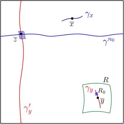
Figure 1. Proof of Theorem B.

Therefore, as $\gamma^{n_{0}}$ and $\gamma_{y}^{\prime}$ cross horizontally and vertically $\mathbb{T}^{2}$ respectively, there is a point $\overline{z}\in\gamma^{n_{0}}\cap\gamma_{y}^{\prime}$. Hence, since $g$ is a local diffeomorphism, we can conclude by the absolute continuity of the stable lamination (Lemma 3.1) that there is a positive Lebesgue measure subset $R_{0}\subset B(\mu_{0})\cap R$, which is impossible. Thus, $\mu$ is ergodic for every $g\in\mathcal{W}$, which proves the result. ∎

References

- [1] M. Andersson, Transitivity of conservative toral endomorphisms, Nonlinearity 29 (2016), 1047–1055.
- [2] M. Andersson, P. Carrasco and R. Saghin, Non-uniformly hyperbolic endomorphisms, arXiv:2206.08295v2, 2022.
- [3] A. Arbieto and C. Matheus, A pasting lemma and some applications for conservative systems, Ergodic Theory and Dynamical Systems 27 (2017), 1399–1417.
- [4] P. Berger and P. Carrasco, Non-uniformly hyperbolic diffeomorphisms derived from the standard map, Comm. Math. Phys. 329 (2014), 239–262.
- [5] J. Bochi, Genericity of zero Lyapunov exponents, Ergodic Theory and Dynamical Systems 22 (2002), 1667–-1696.
- [6] K. Burns and A. Wilkinson, Stable ergodicity of skew products, Ann. scient. Éc. Norm. Sup. 32 (1999), 859–889.
- [7] B. Chirikov, A universal instability of many-dimensional oscillator systems, Physics Reports 52 (1979), 263–379.
- [8] S. Crovosier and E. R. Pujals, Strongly dissipative surface diffeomorphisms, Comment. Math. Helv. 93 (2018), 377–400.
- [9] D. Dolgopyat and Y. Pesin, Every Compact Manifold Carries a Completely Hyperbolic Diffeomorphism, Ergodic Theory and Dynamical Systems 22 (2002), 409–-435.
- [10] M. Grayson, C. Pugh, and M. Shub, Stably Ergodic Diffeomorphisms. Annals of Mathematics 140 (1994), 295–-329.
- [11] V. Janeiro, Existence of non-uniformly hyperbolic endomorphisms in homotopy classes, J. Dyn. Control Syst., https://doi.org/10.1007/s10883-023-09668-8, 2023.
- [12] A. Katok, Bernoulli Diffeomorphisms on Surfaces, Annals of Mathematics, 110 (1979), 529–-547.
- [13] P.-D. Liu, Invariant Measures Satisfying an Equality Relating Entropy, Folding Entropy and Negative Lyapunov Exponents, Communications in Mathematical Physics 284 (2008), 391–406.
- [14] P.-D. Liu and L. Shu, Absolute continuity of hyperbolic invariant measures for endomorphisms, Nonlinearity 24 (2011), 1595–1611.
- [15] E. Mihailescu, Physical Measures for Multivalued Inverse Iterates, J. Stat. Phys. 139 (2010), 800–-819.
- [16] G. Nuñez, D. Obata and J. Rodriguez Hertz, New examples of stably ergodic diffeomorphisms in dimension 3, Nonlinearity 34 (2021), 1352–1365.
- [17] D. Obata, On the stable ergodicity of Berger–Carrasco’s example, Ergodic Theory and Dynamical Systems 40 (2018), 1008–10056.
- [18] V. I. Oseledec, A multiplicative ergodic theorem. Characteristic Ljapunov, exponents dynamical systems, Trudy Moskov. Mat. Obšč 19 (1968), 179–210.
- [19] Y. Pesin, Charateristic Lyapunov exponents and smooth ergodic theory, Rusian Mathematical Surveys 32 (1977), 55–114.
- [20] C. Pugh and M. Shub, Stably ergodic dynamical systems and partial hyperbolicity, J. of Complexity 13 (1997), 125–179.
- [21] M. Qian and S. Zhu, SRB measures and Pesin’s Entropy Formula for Endomorphisms, Transactions of the American Mathematical Society 312 (2002), 1453–1471.
- [22] J. J. Rushanan, Eigenvalues and the Smith normal form, Linear Algebra and its Applications 216 (1995), 177–184.
- [23] A. Tazhibi, Stably ergodic diffeomorphisms which are not partially hyperbolic, Israel Journal of Mathematics 142 (2004), 315–-344.
- [24] M. Viana, J. Yang, Continuity of Lyapunov exponents in the topology, Israel J. Math., 229 (2019), 461–485.