A Bayesian functional PCA model with multilevel partition priors for group studies in neuroscience

Abstract

The statistical analysis of group studies in neuroscience is particularly challenging due to the complex spatio-temporal nature of the data, its multiple levels and the inter-individual variability in brain responses. In this respect, traditional ANOVA-based studies and linear mixed effects models typically provide only limited exploration of the dynamic of the group brain activity and variability of the individual responses potentially leading to overly simplistic conclusions and/or missing more intricate patterns. In this study we propose a novel method based on functional Principal Components Analysis and Bayesian model-based clustering to simultaneously assess group effects and individual deviations over the most important temporal features in the data. This method provides a thorough exploration of group differences and individual deviations in neuroscientific group studies without compromising on the spatio-temporal nature of the data. By means of a simulation study we demonstrate that the proposed model returns correct classification in different clustering scenarios under low and high of noise levels in the data. Finally we consider a case study using Electroencephalogram data recorded during an object recognition task where our approach provides new insights into the underlying brain mechanisms generating the data and their variability.

1 Introduction

Group comparison for neuroscientific data involves comparing sets of spatio-temporal recordings such as those obtained using electroencephalography (EEG), magnetoencephalography or functional Magnetic Resonance Imaging (fMRI) under different conditions. The spatio-temporal nature of the data combined with its multiple levels structure (recording, subject, group) and the inter-individual heterogeneity in brain responses, make the analysis of these data an open challenge in neuroscience. ANOVA-based analyses have been the standard approach for task-based experiments in neuroscience alday2017electrophysiology, . Although well suited for several experimental designs, ANOVA methods in neuroscience have limited the exploration of complex heterogeneous spatio-temporal processes to a simple binary decision (accept/reject) over aggregated measures of the brain signals (e.g. latency, amplitude, power in clinically relevant frequency bands). More recently, the use of complex dynamic stimuli in cognitive neuroscience has driven the choice of statistical methods toward linear mixed-effect models alday2017electrophysiology, ; hasson2012future, . Linear mixed effect models allow more flexible designs and also account for additional variation at multiple levels. Despite the increased flexibility, in general, standard mixed effect models are insufficient for the study of neuroscientific recordings arising from group studies as they are not able to capture how different sources of heterogeneity, such as group effects and individual deviations, vary in time. In this framework, using bespoke advanced methodologies, researchers should be able to extract from the data (a) what the impact of different experimental conditions on the brain activity at different time points are; and (b) how these time-varying effects differ between individuals in the same group. Exploring these intricate patterns will provide neuroscientists with a better and more complete understanding of the underlying brain mechanisms and their variability in the population.

The idea of exploring brain activity from a dynamical perspective has attracted wide interest in the neuroimaging literature in recent years. gonzalez2018task, ; warnick2018bayesian, ; hutchison2013dynamic, Moreover, understanding inter-individual variability in brain functions has become another area of growing research interest in neuroscience. seghier2018interpreting, ; li2017linking, ; zhang2016spatiotemporal, We propose a novel comprehensive model-based approach for the exploration of dynamic brain activity patterns in the context of group studies, namely Bayesian functional Principal Components Analysis (fPCA) with multilevel partition priors. Functional PCA has been successfully employed in neuroscientific studies since the early 2000s. For example, Viviani et al.viviani2005functional, used fPCA for the analysis of fMRI data showing that fPCA is more effective in recovering the signal of interest than standard PCA. Di et al.di2009multilevel, proposed a Multilevel Functional PCA model to extract intra- and inter-subject geometric components of multilevel functional data which was successfully employed to identify and quantify associations between EEG activity during sleep and adverse cardiovascular outcomes. Hasenstab et al.hasenstab2017multi, proposed a multi-dimensional version of fPCA for the analysis of repeated evoked potentials in EEG data showing how the new methodology provided further insights into the learning patterns of children with Autism Spectrum Disorder.

More recently, fPCA has been used within the functional clustering framework to explore complex spatio-temporal patterns.zhang2023review, ; wu2022clustering, Further, Margaritella et al.margaritella2021parameter, have recently shown how combining fPCA and Bayesian model-based clustering can help the exploration of spatio-temporal patterns for different neuroscientific recordings. In this paper, we propose a new method for the analysis of dynamic brain activity and its heterogeneity in the challenging case of group studies. Our method combines fPCA, to extract the most important temporal trends in the data, and a Bayesian nonparametric clustering approach, to simultaneously carry out group comparisons while flexibly assessing heterogeneity in subjects’ brain responses. We make use of the idea of partition priorsdunson2009nonparametric, to develop a novel multilevel partition prior which allows for clustering at different levels in the data; namely between all individuals (common cluster), between subjects of the same group (group-specific clusters) and within individuals (subject-specific clusters). The first two cluster types allow for the identification of different group effects while the latter type captures possible individual deviations. Combined with fPCA, this methodology produces a data-driven selection of clusters at different levels which include potentially different subsets of the individuals studied for different relevant time widows (as identified by the eigendimensions). We show in this paper how this approach returns novel insights on the dynamic brain activity in groups under different experimental conditions and of the associated inter-individual heterogeneity.

The paper is organised as follows: in Section 2 we present the features of the proposed model; in Section 3 we show results of a simulation study to test the model performance under low and high noise levels in the data; results of a case study employing EEG recordings are reported in Section 4; conclusions and further directions are discussed in Section 5.

2 Bayesian functional PCA with multilevel partition priors for group studies

In this section we present the structure of the proposed model and the key features of this approach.

2.1 Hierarchical structure

The following hierarchical structure defines the probability distributions for the data and all the parameters in the model. Each hierarchical level is introduced and commented separately starting from the data level.

Level 1: we assume that data $Y_{ui}(t)$ from $i=1,\dots,n$ recording locations and $t=1,\dots,T$ time points are collected from $u=1,\dots,U$ subjects. Further we assume that $u=1,\dots,U_{A}$ are subjects from group A and $u=U_{A}+1,\dots,U$ are subjects from group B. Groups could represent, for example, patients and controls; or individuals undertaking two different tasks. Following standard functional data analysis (FDA) assumptionsramsay2005functional, , we define the distribution of the centred data $\widetilde{Y}_{ui}(t)$, given the parameters $\xi_{uik}$ of the underlying smooth functions $X_{ui}(t)$ and the noise term $\tau$, to be:

$$\tilde{\textbf{Y}}_{ui}|\textbf{X}_{ui},\tau \sim\text{N}_{\text{T}}(\textbf{X}_{ui},\tau^{-1}\textbf{I}),$$ (1)

$$\textbf{X}_{ui} =\sum_{k=1}^{K}\xi_{uik}\boldsymbol{\phi}_{k},$$

where $\tilde{\textbf{Y}}_{ui}$, $\textbf{X}_{ui}$, and the eigenfunctions $\boldsymbol{\phi}_{k}$ are T-dimensional vectors and $\text{N}_{\text{T}}(\textbf{X}_{ui},\tau^{-1}\textbf{I})$ denotes the probability density function of a multivariate Gaussian random variable with mean $\textbf{X}_{ui}$ and variance-covariance matrix $\tau^{-1}\textbf{I}$, such that I denotes a $T\times T$ identity matrix. The parameters $\xi_{uik}$ are the functional Principal Component scores (fPC scores) and the focus of our analysis. We use a set of common bases for all subjects and curves which permit us to explore variation at different levels through clustering of the fPC scores. The principal component bases have the advantage of being the most efficient bases of size $K$ and, most importantly, they offer a meaningful interpretation in terms of explained variance.ramsay2005functional, The number of bases, $K$, is selected to include the most important bases up to a pre-defined amount of total variation (examples are provided in both the simulation and real data analyses). We assume constant noise for simplicity.

Level 2: to indicate the latent classes and the relative parameters, we introduce a classification variable $z_{uik}$ that identifies which latent class $j$ is associated with parameter $\xi_{uik}$. For each $u,i,k$ with $k=1,\dots,K$, the prior conditional distribution of $\xi_{uik}$, given the parameters of underlying clusters $\big{[}(\mu_{uk1},s_{uk1}),\dots,(\mu_{ukJ},s_{ukJ})\big{]}$ and the classification variable $z_{uik}$, is given by

$$\xi_{uik}|z_{uik},\mu_{ukj},s_{ukj} \sim\text{N}\big{(}\mu_{u\,k,\,j=z_{uik}},s^{-1}_{u\,k,\,j=z_{uik}}\big{)},$$ (2)

where $\mu_{u\,k,\,j=z_{uik}}$ and $s_{u\,k,\,j=z_{uik}}$ are the corresponding mean and precision for the $j$-th cluster of the $u$-th subject in the $k$-th eigendimension, respectively. It is worth noting in Equation (2) that $z_{uik}=z_{u^{\prime}ik}$ and $z_{uik}=z_{ui^{\prime}k}$ do not imply $\xi_{uik}=\xi_{u^{\prime}ik}$ and $\xi_{uik}=\xi_{ui^{\prime}k}$ respectively, but only that these fPC scores share the same cluster means and variances for a given eigendimension $k$. Therefore, our approach allows for both within-subject and inter-subject variability to be considered in our model structure through variability in the fPC scores. We employ a $J-$dimensional mixture of Gaussian distributions, independently for each retained eigendimension $k=1,\dots,K$ to allow for different partitions in each mode of variation. A key role in our model is played by the classification variable $z_{uik}=j$ with $j=1,\dots,J$ defined as:

$$z_{uik} =c^{[1]}_{g_{uk}}+c^{[2]}_{g_{uk}}D_{uk}+c^{[3]}_{g_{uk}}\eta_{uik}\quad.$$ (3)

The indicator vector $\boldsymbol{c}_{g_{uk}}=\left(c^{[1]}_{g_{uk}},c^{[2]}_{g_{uk}},c^{[3]}_{g_{uk}}\right)\in\{(1,0,0),(0,1,0),(0,0,1)\}$, controlled by the random variable $g_{uk}$, is defined such that $c^{[1]}_{g_{uk}}$ corresponds to the label $j=1$ and denotes membership to a common cluster; $c^{[2]}_{g_{uk}}$ corresponds to labels $j=2,3,$ which denote membership to a group-specific cluster (either group A or B, according to a fix indicator $D_{uk}\in\{2,3\}$); and $c^{[3]}_{g_{uk}}$ corresponds to labels $j=4,\dots,J$ which denote membership to a subject-specific cluster, and are allocated according to the variable $\eta_{uik}$. We refer to this partition of labels $\{\{1\},\{2,3\},\{4,\dots,J\}\}$ as the subject-level partition. The variable $\eta_{uik}$ regulates a second level of clustering called recording-level partition to explore clustering of subject-specific recording locations $i=1,\dots,N$ in order to identify possible deviations from the relative group behaviour. To clarify the notation, consider the following example for a specific eigendimension $k$. When two or more subjects from groups A and B share similar patterns in $k$, all their fPC scores receive label 1 and they are clustered together in the common cluster. On the other hand, when two or more subjects from the same group share patterns not found in the other group, their relative fPC scores receive either label 2 (if in group A) or 3 (if in group B) and are clustered together in the relative group-specific cluster. Finally, if a subject shows patterns that are different from those captured by the global clusters (common and group), a second level of clustering, the recording-level partition is activated to assign the subject’s scores to subject-specific clusters (with labels ${4,\dots,J}$) according to the variable $\eta_{uik}$.

Level 3: prior distributions for $\big{[}(\mu_{uk1},s_{uk1}),\dots,(\mu_{ukJ},s_{ukJ})\big{]}$, $g_{uk}$ and $\eta_{uik}$ and the hyperparameters $\phi_{ukj},\,\gamma_{ukj},\,(\omega_{1Dk},\omega_{2Dk},\omega_{3Dk})$ and $(p_{1Dk},\dots,p_{JDk})$, are given by

$$\eta_{uik}|p_{1Dk},\dots,p_{JDk} \sim f_{\text{C}}\big{(}p_{1Dk},\dots,p_{JDk}\big{)},$$ (4)

$$g_{uk}|\omega_{1k},\omega_{2k},\omega_{3k} \sim f_{\text{C}}(\omega_{1k},\omega_{2k},\omega_{3k}),$$

$$\quad\hskip 48.36958pt\mu_{ukj}= \mu_{k1}\quad \mu_{k1} \sim\text{N}(0,h^{-1}_{k1}) \quad\text{for }j =1,$$

$$\quad s^{-1/2}_{ukj}= s^{-1/2}_{k1}\quad s^{-1/2}_{k1} \sim\text{U}(0,\gamma_{k1}) \quad\text{for }j =1,$$

$$\quad\mu_{ukj}= \mu_{kD}\quad \mu_{kD} \sim\text{N}(\phi_{kD},h^{-1}_{kD}) \quad\text{for }j =2,3,$$

$$\quad s^{-1/2}_{ukj}= s^{-1/2}_{kD}\quad s^{-1/2}_{kD} \sim\text{U}(0,\gamma_{kD}) \quad\text{for }j =2,3,$$

$$\mu_{ukj} \sim\text{N}(\phi_{ukj},h^{-1}_{ukj}) \quad\text{for }j =4,\dots,J,$$

$$s^{-1/2}_{ukj} \sim\text{U}(0,\gamma_{ukj}) \quad\text{for }j =4,\dots,J,$$

where $f_{\text{C}}()$ and $\text{U}()$ denote the probability mass function of a categorical random variable and the probability density function of a uniform random variable, respectively. Parameters $(\omega_{1k},\omega_{2k},\omega_{3k})$ control the subject-level partition probabilities in each eigendimension (note that $\sum_{k=1}^{K}\omega_{k}=1$). For example, if $\omega_{11}\approx 1$, all subjects’ fPC scores in eigendimension $1$ would be assigned to the common cluster with mean $\mu_{11}$ and precision $s_{11}$ (or, equivalently, standard deviation $s^{-1/2}_{11}$). In the opposite scenario, $\omega_{31}\approx 1$ would assign all subjects in eigendimension $1$ to subject-specific clusters. When a subject is allocated to a subject-specific cluster, the recording-level partition probabilities $(p_{1Dk},\dots,p_{JDk})$ govern the allocation of each subject’s fPC scores to a potentially different number of clusters, labelled $j\in\{4,\dots,J\}$, and with mean $\mu_{u1j}$, precision $s_{u1j}$ and cluster size controlled by $p_{jD1}$. By making these probabilities dependent on the groups $D$, we account for group-specific differences in the number and size of the subject-specific clusters. Hyperparameters $h,\gamma,\phi$ can be centred around functions of the empirical fPC score estimates.richardson1997bayesian, In practice, using the empirical means and variances of the fPC scores for every group $D$ and dimension $k$ appeared to work well in both the simulation and case study. A detailed summary of the different settings used is reported in Supplementary Materials A.

Level 4: prior distributions for $(\omega_{1k},\omega_{2k},\omega_{3k})$ and $(p_{1Dk},\dots,p_{Dk})$ are given by

$$p^{*}_{1Dk}|\alpha_{k} \sim\text{Beta}(1,\alpha_{k}),$$ (5)

$$p_{1Dk}=\dfrac{p^{*}_{1Dk}}{\sum_{j=1}^{J}p^{{}^{\prime}}_{jDk}}; \quad p_{jDk}=\dfrac{p^{*}_{jDk}\prod_{l<j}(1-p^{*}_{lDk})}{\sum_{j=1}^{J}p^{*}_{jDk}},$$

$$\boldsymbol{\omega}_{k} \sim\text{Dir}\bigg{(}\delta_{1},\delta_{2},\delta_{3}\bigg{)},$$

where $\text{Dir}()$ represents the Dirichlet distribution. Setting $\delta_{1}=\delta_{2}=\delta_{3}$ produces no prior advantage between the three cluster types (common, group-specific and subject-specific) but, in practice, setting $\delta_{1}=\delta_{2}<\delta_{3}$ offers a prior better aligned to the usual prior beliefs of a group study (equal prior probability of common vs group effects and low chance of subject-specific deviations). The parameters $\boldsymbol{p}_{Dk}$ follow the stick-breaking constructionsethuraman1994constructive, with parameter $\alpha_{k}$ modelling the prior belief over the mixing proportions $p_{1Dk},\dots,p_{JDk}$. The dispersion parameter $\alpha$ is usually fixed or modelled with a prior distribution. Both the expected number of clusters and their variance can be obtained for fixed $\alpha_{k}$ and number of recording sites $n$ or by averaging out the prior distribution for $\alpha_{k}$.escobar1994estimating, ; jara2007dirichlet, We used $\alpha_{k}=1$ as it represents our prior belief that a limited number of clusters is expected to arise in a subject’s recording and we let this expectation gradually grow with the number of recoding sites $n$. Details of the choice of $\delta$s and $\alpha$ are reported in Supplementary Materials A. In practice, a simulation study should be conducted to assess the sensitivity of the posterior estimates to the priors specified.
The complete model structure can be displayed with a direct acyclic graph (DAG, Figure 1). Sampling from the joint posterior distribution of all parameters is obtained using Markov Chain Monte Carlo (MCMC) samplers. We employ the rnimble package to run the model with NIMBLE in R using MCMC.NIMBLE, ; NIMBLEr, In the next two sections we provide examples of how our method can be applied to a range of different scenarios. All analyses have been implemented in R code that will be available online upon publication.^a

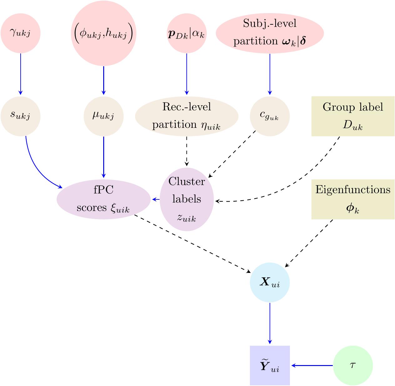
Figure 1: The structure of our proposed model shown with a Direct Acyclic Graph (DAG). Squares= observed random variables; circles= unobserved random variables; dashed= deterministic relationship; solid= stochastic relationship. Rec.-level and Subj.-level are abbreviations for Recording-level and Subject-level partitions, respectively.

3 Simulation study

We perform a Monte Carlo simulation study to assess the performance of the proposed model in curve classification between common, group and subject-specific clusters for different levels of noise in the data. We consider a simulation setting consisting of 40 subjects enrolled in two equally-sized study groups, denoted A and B. To generate the spatio-temporal datasets for all these individuals, we employ two eigenfunctions (Figure 2, top row) to generate brain recording-like patterns in the curves as shown in the bottom row of Figure 2. For each subject $u=1,\dots,40$, we generate data in the form of $t=1,\dots,150$ time-points for $n=1,\dots,50$ recording locations. The dimensionality of the overall dataset is therefore $40\times 50\times 150$.

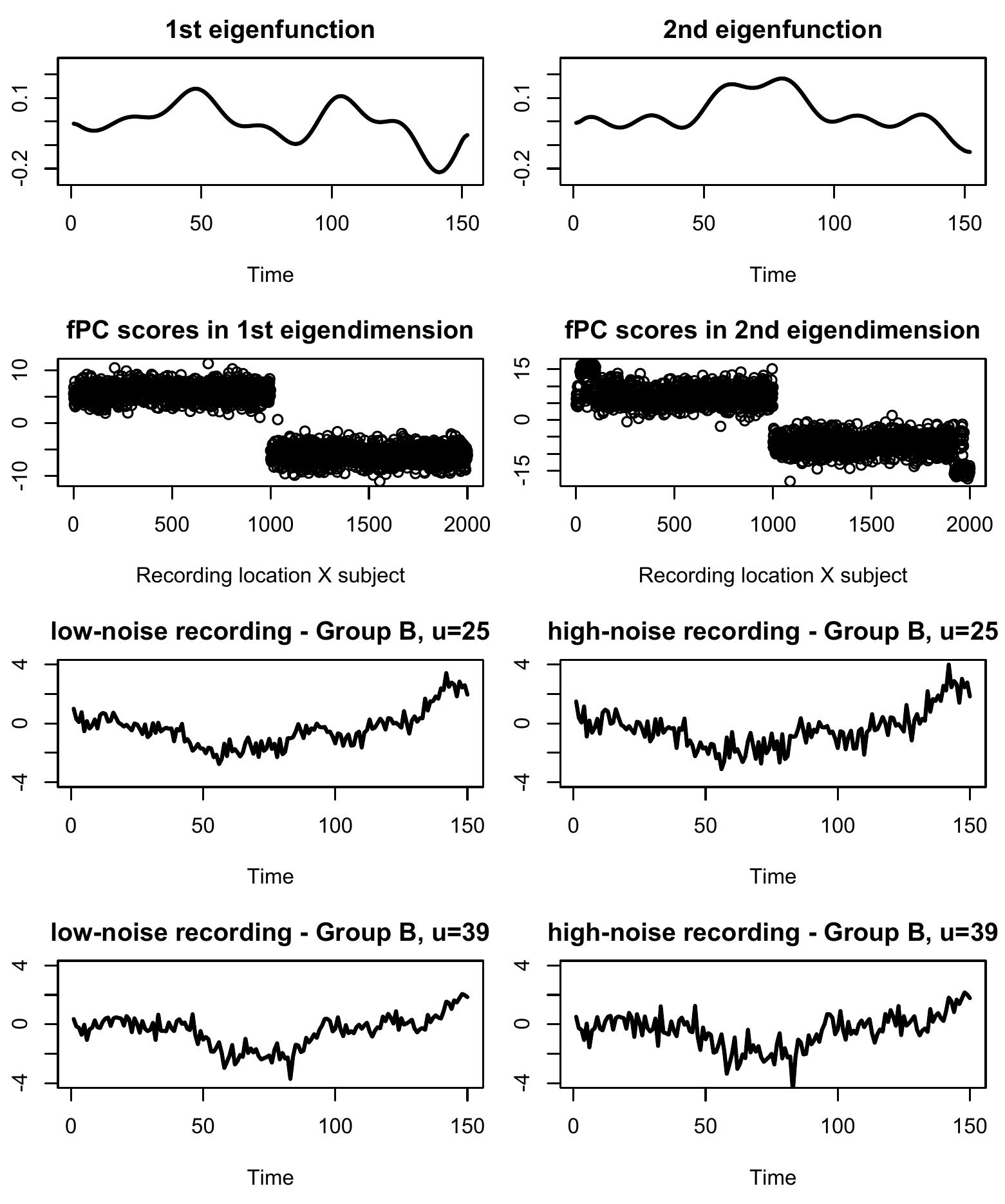
Figure 2: Simulation study: eigenfunctions (1st row), fPC scores used for all subjects and recording locations (2nd row), and two examples of the synthetic recordings obtained with different noise levels (3rd and 4th rows).

Group clusters are assumed to be different between groups in both eigendimensions but, within each of the two groups, we select a small subset of individuals to have outlying patterns in their recordings as generated by a different structure in their fPC scores distribution. Specifically, two subjects in group A and B ($u=1,2,39,40$) present two clusters in their fPC scores in the second eigendimension (Figure 2). We apply a random Gaussian noise and consider models with two different noise levels (low noise: signal-to-noise ratio (SNR)=6 and high noise: SNR=2). The bottom plots in Figure 2 show an example of the curves obtained by adding either low or high random noise to the smooth data. The hyperparameter values used to run the model are listed in Supplementary Material A. The MCMC simulations were run for $20\times 10^{3}$ iterations and the first $10\times 10^{3}$ were discarded as burn-in (This appeared to be a conservative estimate for the burn-in). The average computational time was 50 minutes (SD= 3 minutes) as measured by a computer with 8 cores, 64 GB RAM and a M1 processor. We generated 100 datasets to use in our study.

Clustering performance was assessed using two different methods: the Adjusted Rand Index (ARI) and the Variation of Information (VI).hubert1985comparing, ; wade2018bayesian, The ARI is used in the literature to evaluate clustering performance using maximum a posteriori probabilities to quantify the similarity between the estimated partitions and the ground truth.hubert1985comparing, ; mcdowell2018clustering, We also employed similarity matrices to obtain a clustering point estimation via the VI approach.This method overcomes known limitations of the ARI, namely a tendency of the optimal partition to overestimate the number of clusters. In addition, we make use of credible balls to explore the uncertainty around the partition point estimate. A credible ball summarizes the posterior uncertainty around a clustering estimate and is defined as the smallest ball with posterior probability of at least 1-alpha. Further details can be found in Wade and Ghahramani.wade2018bayesian,

3.1 Simulation results

In this section, we report the results of the simulation study for the two noise-level scenarios and eigendimensions.

Low noise, eigendimension 1: there were 2 group-specific clusters in the first eigendimension. Classification using ARI produced correct classification (ARI=1) in 93 out of 100 simulations. For the other seven simulated datasets, the model returned an ARI of 0.95 and 0.91 in four and three datasets corresponding to 1 and 2 subject misclassified, respectively. Using VI, correct classification was obtained in 97 simulations while 1 subject was misclassified in the remaining 3 simulations. Variation measured with 95% cluster balls indicated very low cluster uncertainty: only five of the 97 simulations that correctly classified the subjects identified alternative partitions within the 95% cluster ball where the fPC scores of either one or two subjects in group B were allocated to subject-specific clusters.

Low noise, eigendimension 2: there were 2 group-specific and 4 subject-specific clusters in the second eigendimension. Classification using both ARI and VI returned the correct partition in all 100 simulations. The 95% cluster balls indicated very low cluster uncertainty: only one simulation identified an alternative classification where one additional subject in group B was allocated to subject-specific clusters. Subject-specific clustering of the 50 recording locations returned low classification error with two third of the simulated datasets returning zero or a single classification error and two or three errors in one third of the datasets.

High noise, dimension 1: under high noise (STN=2), ARI returned exact classification (ARI=1) in 62 out of 100 simulations, misclassified one subject in 23 simulations (ARI= 0.95), two subjects in 14 simulations (ARI= 0.90) and three subjects in 1 simulation (ARI=0.87). Using VI, all individuals were correctly classified in 77 simulations; one individual was misclassified in 15 simulations; and two individuals were misclassified in 8 simulations. The three misclassified subjects were among those with individual-specific clusters in the second eigendimension. Five simulations with misclassified individuals included the true partition within their 95% cluster ball. The 95% cluster balls indicated very low cluster uncertainty: only 5 of the 77 simulations that correctly classified the subjects identified alternative partitions within the 95% cluster ball where either one or two subjects in group B were allocated to subject-specific clusters.

High noise, dimension 2: Classification using both ARI and VI returned correct classification in all 100 simulations. The 95% cluster balls indicated again very low cluster uncertainty: only two simulations identified alternative classifications where one additional subject in group B was allocated to subject-specific clusters. Subject-specific clustering of the 50 recording locations returned again low classification error with 60% and 40% of the simulated datasets returning zero to a single classification error and two to three errors, respectively.

Overall, the model showed very good to optimal performance in retrieving the correct partitions in both eigendimensions and different noise levels, particularly when the VI was used. When the correct partition was identified, there was always low cluster uncertainty around it, with only one or two additional subjects allocated to subject-specific clusters within the 95% cluster ball. A higher noise level led only to a moderate increase in the misclassification for both subject-level and recording-level partitions. In the next section, we apply our model on a different challenging scenario using a real neuroscientific dataset which featured both a smaller sample size and a potentially higher inter-individual variability in the recordings.

4 Case study: Event-related potentials data

We consider data from an EEG study on brain activations following object recognition tasks.zhang1995event, Event-Related Potentials (ERPs) continue to be a popular electrophisiological tool to investigate memory functions under both physiological and pathological conditions (see for example these studies yan2023effect, ; saltzmann2022neural, ; stevens4208065relational, ). Small bio-electrical signals are generated by the brain in response to specific events or stimuli. These signals are time locked to cognitive events thus providing a non-invasive approach to study psychophysiological correlates of mental processes.sur2009event, The subjects were shown two separate images taken from the 1980 Snodgrass and Vanderwart picture.snodgrass1980standardized, The second stimulus was either a different image (unmatched) or the same image (matched). The data were recorded using a cap with 64 electrodes placed on the subject’s scalp and the brain activity at each recording electrode was sampled at 256 Hz for 1 second. Further details on the recording setting can be found in Zhang et al.zhang1995event, Data are available from the UC Irvine Machine Learning Repository website.EEGData,

We focus our analysis on the first 300 milliseconds (77 time points) recorded in the occipital region of the brain where the visual cortex is located.crossman2018neuroanatomy, In particular, we explore whether our approach offers additional insights into the spatio-temporal differences and the inter-subject variability in the ERPs recorded from this area.

For each subject, multiple repetitions of the tasks are averaged to amplify the underlying evoked response. The resulting potentials are visually inspected to ascertain the presence of the evoked signals and eliminate recordings affected by artifacts. Three components are expected at approximately 110, 175 and 247 milliseconds (named C110, C175 and C247).zhang1995event, Following standard terminology, an epoch identifies a time-window extracted from the continuous EEG signal of an individual under either condition while negative and positive ERP peaks identify convex and concave trajectories, respectively. The final dataset includes 20 epochs, 60 recordings per stimulus from 10 subjects. Smoothed data of 4 individuals are shown in Figure 3, where ERPs following matched stimuli and unmatched stimuli are shown in black (solid) and red (dashed), respectively. The complete dataset is shown in Supplementary Materials C.

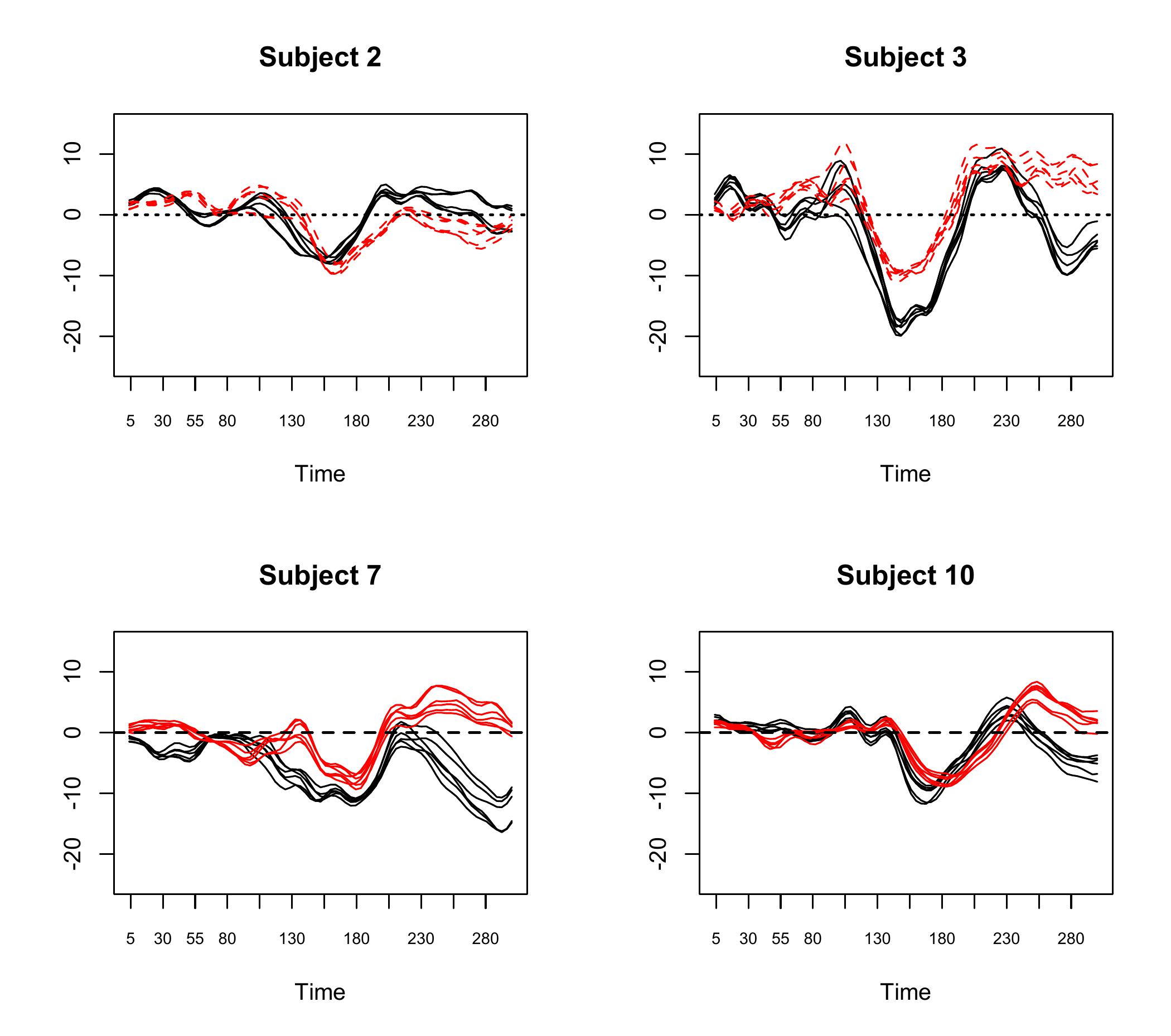
Figure 3: ERPs study: an example of recordings from four subjects included in the analyses. ERPs recorded during matched stimuli are in black (solid), those recorded during unmatched stimuli are in red (dashed).

A final ($120\times 77$) dataset is input to fPCA for curve smoothing and dimension reduction using the pca.fd function from the fda package in R.fdapackage, We retained the first three dimensions explaining almost $80\%$ of the total variability while accounting for more than $15\%$ each. The smoothed recordings and the first two retained eigendimensions are shown in Figure 4 while the third eigendimension is shown in Figure 2 of Supplementary Materials C. We used the model settings described in Section 2 while in Supplementary Materials B we present the result of a sensitivity analysis where the impact of choosing different hyperparameter values is explored. Convergence was assessed using trace plots and Brooks-Gelman-Rubin diagnostics and chain length was monitored using the effective sample size (see Supplementary Materials D for further details). The computational time to run $2\times 10^{5}$ iterations (discarding the first $10^{5}$ as burn-in) using NIMBLE on a Quad-core Intel CPU running at 2 GHz with 16 GB RAM was 90 minutes.

4.1 ERPs analysis results

The results of the ERPs study are presented separately for each of the three eigendimensions analysed to gain insights into local features of the recordings. For each dimension, we explore how subjects’ recordings were allocated between common, group, and subject-specific clusters. Table 1 reports the partitions obtained in each eigendimension and their relative 95% cluster balls. The three point estimates take most of the variation within the relative cluster balls with only minor or negligible deviations in the first and the other two eigendimensions, respectively.

Dimension 1: This eigendimension is mostly related to variability of approximately the last 70 ms of the recording (Figure 4, bottom-right panel). Our model allocated 50% of the subjects’ recordings to group clusters (10 epochs, 4 in the matched and 6 in the unmatched condition) with a positive peak in the matched group and a negative peak in the unmatched group (Figure 5, left panel). The recordings of the remaining 50% of individuals were included in the common cluster. No subject-specific pattern was detected. This result was particularly robust to changes in the hyperparameter values (see sensitivity analysis in Supplementary Materials B).

Dimension 2: The second eigendimension represents local variability between 75-175 ms (Figure  4, bottom-left panel). The model allocated 30% of the subjects’ recordings to group clusters (6 epochs, 3 for each condition) with a positive peak in the matched group and a negative in the unmatched group (Figure 5, right panel). The recordings of 8 subjects were allocated to the common cluster (4 for each condition) while the remaining recordings of 6 individuals were allocated to subject-specific clusters (3 for each condition); of these, three subjects in the matched condition presented an opposite peak to that of the respective group cluster while three subjects in the unmatched condition showed the same pattern of their group but with extremely pronounced peaks.

Dimension 3: The third eigendimension includes local variability at 90-130 ms and 180-250 ms (Figure 2 in Supplementary Materials C). The recordings of 55% subjects were allocated to group clusters (11 epochs, 6 in the matched condition and 5 in the unmatched condition) with a positive peak in the matched group and a slightly less pronounced positive peak in the unmatched group. The recordings of the other 35% and 10% of subjects were allocated to common and subject-specific clusters, respectively (Figure 3 in Supplementary Materials C). The recordings of the two individuals allocated to individual-specific clusters showed an inverted peak in the recordings compared to that of the respective group cluster.

Overall, dimensions 1 and 3 presented the largest group clusters, including the recordings of 50% and 55% of subjects respectively, and the fewest individual-specific clusters (only 2 subjects in dimension 3). Conversely, dimension 2 showed the smallest group clusters (including only 6 subjects) and the largest number of individual-specific clusters (6 subjects). The latter result was also confirmed in the sensitivity analysis (Supplementary Materials B). These results are in agreement with the original study of Zhang et al.zhang1995event, but provide further understanding on the heterogeneity of ERP responses in the occipital lobe, following matched vs unmatched visual stimuli. The group patterns identified in the first dimension capture the difference in the latency of the component at 247ms (C247) between matched and unmatched trials as found by Zhang et al.zhang1995event, and in a similar experiment also by Begleiter et al.begleiter1993neurophysiologic, This pattern explained approximately $40\%$ of the total variability in our sample.

Results of our analysis suggested that stimulus-specific brain responses in the occipital lobe became highly synchronised between 230ms and 300ms. However, only half of the recordings were allocated to group-specific clusters while the other 50% were pooled together in the common cluster, suggesting that the effect of non-matching stimuli on the latency of the C247 component in the occipital lobe might be a trait not consistent in the population. The group pattern identified in the second dimension corresponds to a longer latency of the C110 component during non-matching stimuli. This result was not found in Zhang et al.zhang1995event, but it is in agreement with the study of Begleiter et al.begleiter1995event, In our analysis, the highest individual heterogeneity in the trajectories was found associated to this component, with 30% of the subjects’ recordings being classified in subject-specific clusters (which might explain why the group effect was not originally identified by Zhang et al).zhang1995event, Interestingly, subject-specific clusters in the matched group included markedly inverted peaks while those in the unmatched group had much less extreme patterns, suggesting large heterogeneity around the C110 component might be mostly elicitealpd by the matched condition. In the third eigendimension, half of the recordings were again assigned to group clusters although the clusters means have different magnitude but the same sign. Notably, one subject’ recordings were allocated to subject-specific clusters under both conditions (Subject 3, see Figure 1 in Supplementary Materials C). As the variability explained by this eigendimension is only 17% of the total variation, most of this variation could have been generated by a single individual, as Figure 3 in Supplementary Materials C also suggests. Considering that only the initial eigendimensions capture general patterns in the data, these results suggest limiting the interpretation of our model output to the first two eigendimensions.

In summary, our results indicate that group differences in occipital ERPs elicitealpd by the specific visual tasks analysed arise at a local level (dimension 1 and 2) rather than over the whole recording and could be detected only on subsets of the individuals analysed, the largest being 10 individuals (50%) in the first dimension. Moreover, we found that heterogeneity in subjects’ brain responses change over the length of the EEG recordings. It is highest and presents stimulus-specific differences between 75ms and 175ms (dimension 2), while it is lowest after 230ms (dimension 1). The identification of these complex spatio-temporal patterns highlights the insights that can be gained by exploring brain recordings in group studies using our proposed method.

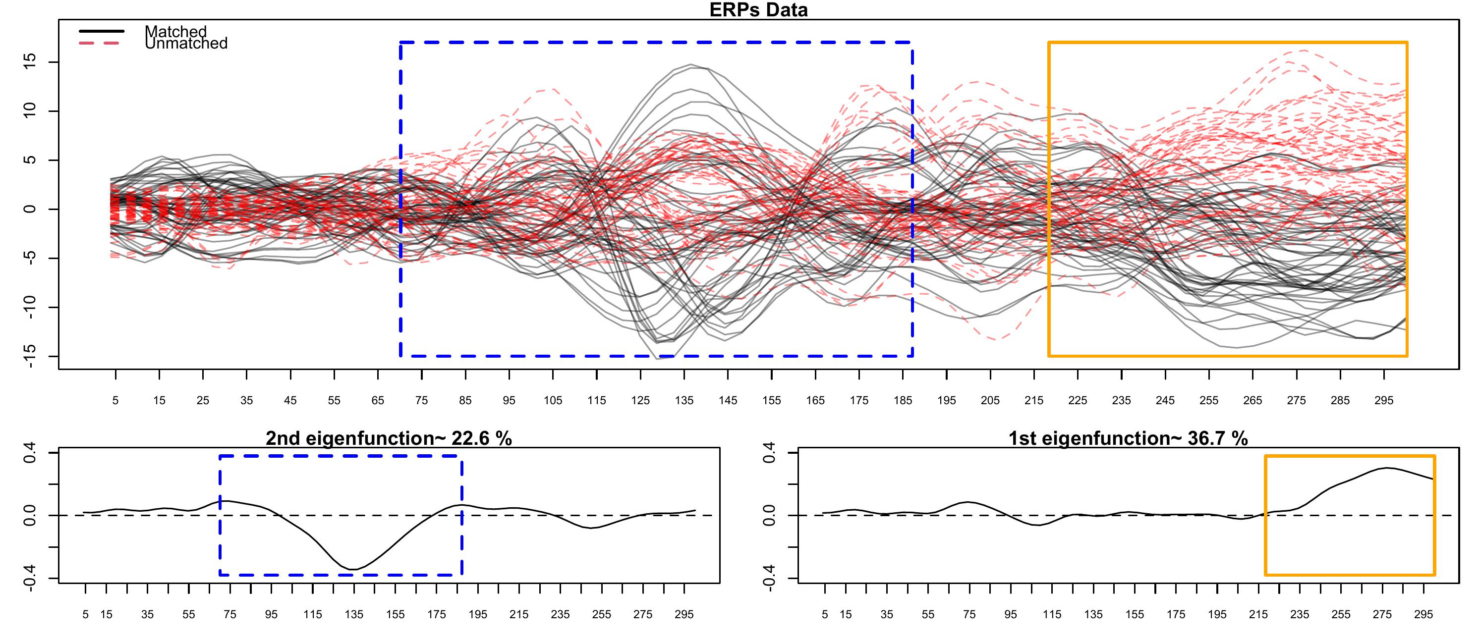
Figure 4: ERPs study: matched (solid) and unmatched (dashed) trajectories. The boxes highlight areas of higher variability described by the first (solid) and second (dashed) eigendimensions.

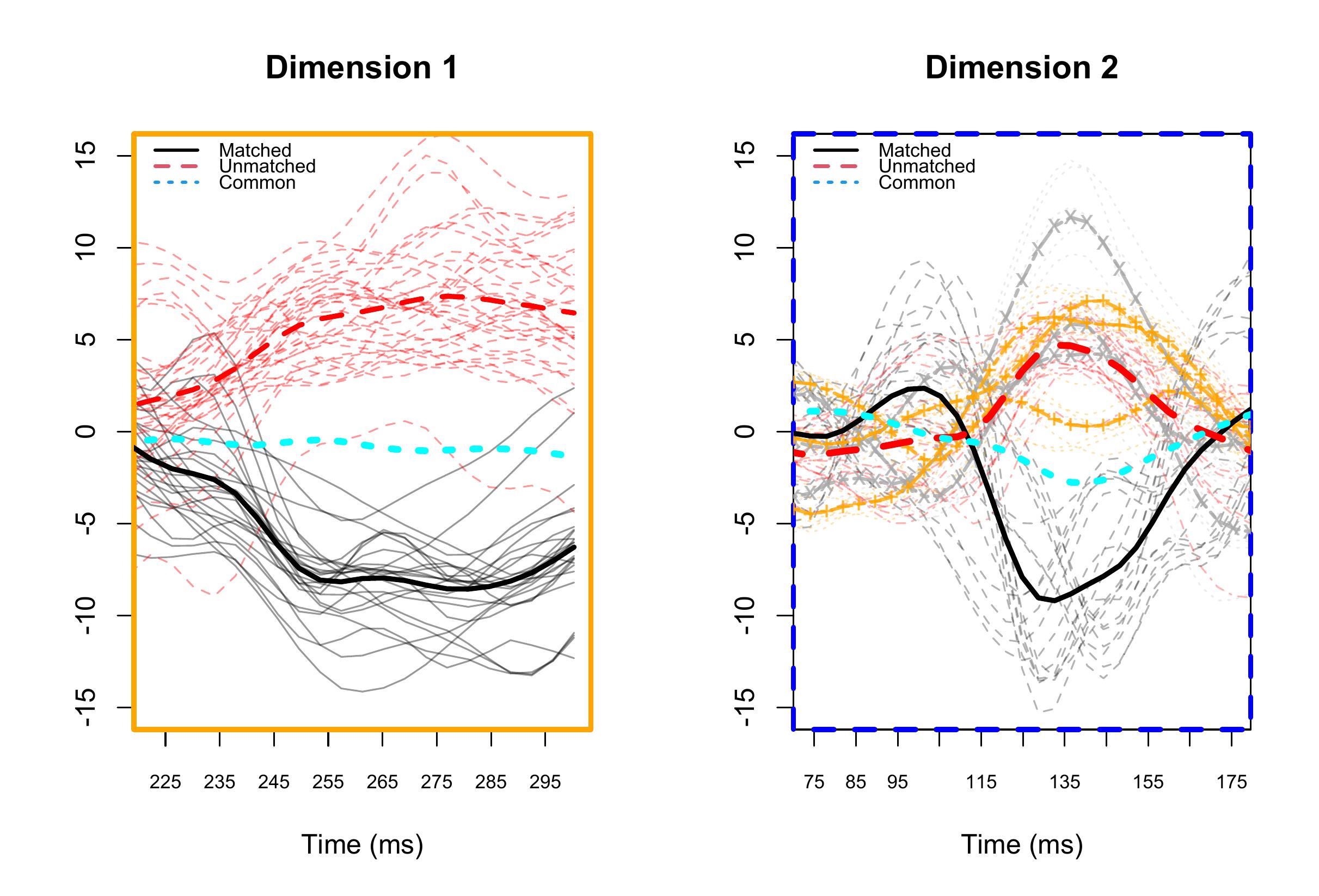
Figure 5: ERPs study: local group differences between matched (solid) and unmatched (dashed) recordings identified by the model in the first two eigendimensions. In bold the common and group cluster means are superimposed on the relative recordings. The symbols x (grey) and ’$+$’(orange) identify individual-specific cluster means.

5 Discussion

We introduce a novel approach based on a Bayesian functional Principal Components Analysis model and a modified Dirichlet Process mixture prior to explore the spatio-temporal features of neuroscientific recordings and investigate inter-subject heterogeneity in the analysis of groups.

The proposed method allows for an in-depth exploration of local patterns arising from complex spatio-temporal data recorded from experimentally designed groups (e.g. patients vs controls, pre vs post task/treatment). By using the eigenfunctions as smooth constituent blocks of the recorded signal, we focused the analyses on only the most important temporal features in the data. The data-driven trade-off between subject-level and recording-level partitions of the fPC scores allows for a flexible exploration of both group-specific behaviours and inter-individual variability. This returns an in-depth analysis of the whole multilevel spatio-temporal dataset where a subject might share some of the temporal features of their recordings either with individuals from all groups or from their own group only or with no one else.

Simulation results showed that the method proposed returns correct classification, with both low and high noise levels in the data with the latter introducing some minor degree of misclassification. As expected, using the Variation of Information proposed by Wade et al.wade2018bayesian, produced more reliable classification under both STN ratios, compared to the Adjusted Rand Index. Interestingly, the misclassification observed affected the first eigendimension only. We believe this could be the result of using a global smoothing approach on non-homogeneous dependent curves affected by high noise. The consequence for classification observed was a tendency to assign one or two individuals to subject-specific clusters beyond the eigendimension where this allocation was correct. Therefore, smoothing at group or subject level could be employed to account for differences in STN ratio among these. Local smoothing could also be considered to account for heteroschedasticity in the recordings. Several local smoothers are available (e.g. local Cross Validation, local Generalised Cross Validation).loader2006local, Although these methods are considered challenging especially when high noise and complex structures characterise the data, they are still an active area of research.grzesik2017local, The results of the case study on ERPs data not only were in agreement with the relevant literaturezhang1995event, ; begleiter1995event, ; begleiter1993neurophysiologic, but also offered additional insights on the underlying complex spatio-temporal process. In particular, we were able to find group differences between matched/unmatched stimuli and link them to specific temporal features. In addition, by looking at the composition of the different clusters we uncovered how individual heterogeneity varied across the main temporal modes of variation in the data. From a practical point of view, our method requires a series of pre and post analyses checks (tuning of hyperparameters values, MCMC checks, sensitivity analysis) that go beyond those required for standard ANOVAs and Linear Mixed Models. Nevertheless, as recording of large and complex datasets is becoming the standard practice, researchers can take a deeper look into the mechanisms governing many biological phenomena as long as they adopt methods that can capture the complexity of such mechanisms. In this respect, our method offers a much more intricate but complete picture of the underlying brain activity compared to the results of the original studies.

There are many interesting research avenues that can be taken to expand this methodology further. One important research direction concerns groups. In our multilevel model we considered two known groups such as patients and controls or treatment A and B. However, there are many cases where groups are unknown and interest may lie in finding them. For example in the identification of different courses in diseases with heterogeneous manifestations as well as in the identification of prognostic patterns in multimorbidity studies. To tackle these challenges it is possible to extend our model to allow for the discovery of unknown groups via a variety of multilevel Dirichlet Process structures such as the Nested DProdriguez2008nested, , the Hierarchical DPteh2006w, or the Multilevel clustering Hierarchical DPwulsin2012hierarchical, . Another timely research direction concerns the applicability of the proposed method to the analysis of large to very large datasets. Given the current trend of technological advancements, the fast accumulation of large quantities of information and their easy access, it is essential to develop scalable methodologies that can compete computationally with machine learning approaches while permitting a more complex analysis of patterns and uncertainty in the data. In this regard, divide-and-conquer and subsampling methods represent a promising research areas for the study of large datasets (see for example these studies king2022large, ; su2020divide, ; song2020distributed, ; quiroz2018speeding, ). In our future research we aim to explore how these methods could be adapted to implement our modelling strategy on large neuroscientific datasets. This study was supported by an Early Career Fellowship of the London Mathematical Society (LMS) [ECF-1920-40].

The Authors declare that there is no conflict of interest.

Note

^a Available at https://github.com/NicMargaritella/BfPCA_MPP

Table 1: ERPs study: the 3 panels show the partitions obtained within each of the 3 eigendimensions studied (C=common, Gm=matched group, Gu=unmatched group, S=subject-specific). Each panel reports the point estimate and the relative three bounds of the 95% credible ball (upper, lower, horizontal; see Wade and Ghahramaniwade2018bayesian, for further details). Within each bound, the differences with the point estimate are highlighted in bold. At the bottom of each panel it is shown the frequency of the different partitions found within the credible ball.

1st eigendimension
Point estimate		95% CB v. upperb.		95% CB v. lowerb.		95% CB horizb.
C:	1m, 2m, 3m,			C:	1m, 3m, 4m,	C:	1m, 3m, 4m,
	4m, 9m, 10m,				9m, 10m, 1u,		9m, 10m, 1u,
	1u, 2u, 5u,				2u, 5u, 6u		2u, 5u, 6u
	6u
Gm:	5m, 6m, 7m,		$\boldsymbol{\equiv}\text{Point estim.}\quad\,\,\,$	Gm:	5m, 6m, 7m,	Gm:	5m, 6m, 7m,
	8m				8m		8m
Gu:	3u, 4u, 7u,			Gu:	3u, 4u, 7u,	Gu:	3u, 4u, 7u,
	8u, 9u, 10u				8u, 9u, 10u		8u, 9u, 10u
S:	$\emptyset$			S:	2m	S:	2m
	Frequency:		$100\%$		$6\%$		$6\%$

2nd eigendimension
Point estimate		95% CB v. upperb.		95% CB v. lowerb.		95% CB horizb.
C:	2m, 6m, 7m,	C:	2m, 7m, 9m,	C:	7m, 9m, 5u,	C:	7m, 9m, 3u,
	9m, 3u, 5u,		3u, 5u, 6u,		6u,8u		6u, 8u, 5u,
	6u, 8u		8u, 9u
Gm:	3m, 5m, 8m	Gm:	3m, 5m, 6m,	Gm:	$\emptyset$	Gm:	3m, 5m, 6m
			8m
Gu:	2u, 4u, 7u	Gu:	2u, 4u, 7u,	Gu:	2u, 4u, 7u	Gu:	2u, 4u, 7u,
			10u				9u
S:	1m, 4m, 10m,	S:	1m, 4m, 10m,	S:	1m, 2m, 3m,	S:	1m, 2m, 4m,
	1u, 9u, 10u		1u		4m, 5m, 6m,		8m, 1u, 10u
					8m, 10m, 1u,
					3u, 9u, 10u
	Frequency:		$<1\%$		$<1\%$		$1\%$

3rd eigendimension
Point estimate		95% CB v. upperb.		95% CB v. lowerb.		95% CB horizb.
C:	2m, 8m, 10m,	C:	1m, 2m, 3m,	C:	10m, 2u, 7u,	C:	1m, 8m, 10m,
	2u, 7u, 8u,		8m, 8u		9u		2u, 7u, 9u,
	9u						10u
Gm:	1m, 4m, 5m,	Gm:	4m, 5m, 6m,	Gm:	5m, 7m, 9m	Gm:	5m, 6m, 7m,
	6m, 7m, 9m		7m, 9m				9m
Gu:	1u, 4u, 5u,	Gu:	1u, 2u, 4u,	Gu:	5u, 6u, 10u	Gu:	1u, 4u, 5u,
	6u, 10u		5u, 6u, 7u,				6u
			9u, 10u
S:	3m, 3u	S:	3u	S:	1m, 2m, 3m,	S:	2m, 3m, 4m,
					4m, 6m, 8m,		3u, 8u
					1u, 3u, 4u,
					8u
	Frequency:		$<1\%$		$<1\%$		$<1\%$

References

- (1) Alday PM, Schlesewsky M and Bornkessel-Schlesewsky I. Electrophysiology reveals the neural dynamics of naturalistic auditory language processing: event-related potentials reflect continuous model updates. eNeuro 2017; 4(6).
- (2) Hasson U and Honey CJ. Future trends in neuroimaging: Neural processes as expressed within real-life contexts. NeuroImage 2012; 62(2): 1272–1278.
- (3) Gonzalez-Castillo J and Bandettini PA. Task-based dynamic functional connectivity: Recent findings and open questions. Neuroimage 2018; 180: 526–533.
- (4) Warnick R, Guindani M, Erhardt E et al. A Bayesian approach for estimating dynamic functional network connectivity in fMRI data. Journal of the American Statistical Association 2018; 113(521): 134–151.
- (5) Hutchison RM, Womelsdorf T, Allen EA et al. Dynamic functional connectivity: promise, issues, and interpretations. Neuroimage 2013; 80: 360–378.
- (6) Seghier ML and Price CJ. Interpreting and utilising intersubject variability in brain function. Trends in Cognitive Sciences 2018; 22(6): 517–530.
- (7) Li R, Yin S, Zhu X et al. Linking inter-individual variability in functional brain connectivity to cognitive ability in elderly individuals. Frontiers in Aging Neuroscience 2017; 9: 385.
- (8) Zhang L, Guindani M, Versace F et al. A spatiotemporal nonparametric Bayesian model of multi-subject fMRI data. The Annals of Applied Statistics 2016; 10(2): 638–666.
- (9) Viviani R, Grön G and Spitzer M. Functional principal component analysis of fMRI data. Human Brain Mapping 2005; 24(2): 109–129.
- (10) Di CZ, Crainiceanu CM, Caffo BS et al. Multilevel functional principal component analysis. The Annals of Applied Statistics 2009; 3(1): 458.
- (11) Hasenstab K, Scheffler A, Telesca D et al. A multi-dimensional functional principal components analysis of EEG data. Biometrics 2017; 73(3): 999–1009.
- (12) Zhang M and Parnell A. Review of clustering methods for functional data. ACM Transactions on Knowledge Discovery from Data 2023; 17(7): 1–34.
- (13) Wu H and Li YF. Clustering spatially correlated functional data with multiple scalar covariates. IEEE Transactions on Neural Networks and Learning Systems 2022; .
- (14) Margaritella N, Inácio V and King R. Parameter clustering in Bayesian functional principal component analysis of neuroscientific data. Statistics in Medicine 2021; 40(1): 167–184.
- (15) Dunson DB. Nonparametric Bayes local partition models for random effects. Biometrika 2009; 96(2): 249–262.
- (16) Ramsay J and Silverman BW. Functional Data Analysis. Springer Series in Statistics, 2005.
- (17) Richardson S and Green PJ. On Bayesian analysis of mixtures with an unknown number of components (with discussion). Journal of the Royal Statistical Society: Series B (Statistical Methodology) 1997; 59(4): 731–792.
- (18) Sethuraman J. A constructive definition of Dirichlet priors. Statistica Sinica 1994; 4(2): 639–650.
- (19) Escobar MD. Estimating normal means with a Dirichlet process prior. Journal of the American Statistical Association 1994; 89(425): 268–277.
- (20) Jara A, García-Zattera MJ and Lesaffre E. A Dirichlet process mixture model for the analysis of correlated binary responses. Computational Statistics & Data Analysis 2007; 51(11): 5402–5415.
- (21) de Valpine P, Turek D, Paciorek C et al. Programming with models: writing statistical algorithms for general model structures with NIMBLE. Journal of Computational and Graphical Statistics 2017; 26: 403–413. 10.1080/10618600.2016.1172487.
- (22) de Valpine P, Paciorek C, Turek D et al. NIMBLE: MCMC, Particle Filtering, and Programmable Hierarchical Modeling, 2022. 10.5281/zenodo.1211190. URL https://cran.r-project.org/package=nimble. R package version 0.12.2.
- (23) Hubert L and Arabie P. Comparing partitions. Journal of Classification 1985; 2(1): 193–218.
- (24) Wade S and Ghahramani Z. Bayesian cluster analysis: Point estimation and credible balls (with discussion). Bayesian Analysis 2018; 13(2): 559–626.
- (25) McDowell IC, Manandhar D, Vockley CM et al. Clustering gene expression time series data using an infinite Gaussian process mixture model. PLoS Computational Biology 2018; 14(1): e1005896.
- (26) Zhang XL, Begleiter H, Porjesz B et al. Event related potentials during object recognition tasks. Brain Research Bulletin 1995; 38(6): 531–538.
- (27) Yan C, Ding Q, Li Y et al. Effect of retrieval reward on episodic recognition with different difficulty: ERP evidence. International Journal of Psychophysiology 2023; 183: 41–52.
- (28) Saltzmann S, Moen K, Chaisson F et al. Neural correlates of task-irrelevant feature processing in visual working memory. Journal of Vision 2022; 22(14): 3567–3567.
- (29) Stevens KL, Teich CD, Longenecker JM et al. Relational memory function in schizophrenia: Electrophysiological evidence for early perceptual and late associative abnormalities. Schizophrenia Research 2023; 254: 99–108.
- (30) Sur S and Sinha V. Event-related potential: An overview. Industrial Psychiatry Journal 2009; 18(1): 70.
- (31) Snodgrass JG and Vanderwart M. A standardized set of 260 pictures: norms for name agreement, image agreement, familiarity, and visual complexity. Journal of Experimental Psychology: Human Learning and Memory 1980; 6(2): 174.
- (32) Begleiter H. EEG Database. UCI Machine Learning Repository, 1999. DOI: https://doi.org/10.24432/C5TS3D, accessed: 2023-12-12.
- (33) Crossman AR and Neary D. Neuroanatomy E-book: An Illustrated Colour Text. Elsevier Health Sciences, 2018.
- (34) Ramsay JO, Graves S and Hooker G. fda: Functional Data Analysis, 2020. URL https://CRAN.R-project.org/package=fda. R package version 5.1.4.
- (35) Begleiter H, Porjesz B and Wang W. A neurophysiologic correlate of visual short-term memory in humans. Electroencephalography and Clinical Neurophysiology 1993; 87(1): 46–53.
- (36) Begleiter H, Porjesz B and Wang W. Event-related brain potentials differentiate priming and recognition to familiar and unfamiliar faces. Electroencephalography and Clinical Neurophysiology 1995; 94(1): 41–49.
- (37) Loader C. Local Regression and Likelihood. Springer Science & Business Media, 2006.
- (38) Grzesik K. Local Cross-Validated Smoothing Parameter Estimation for Linear Smoothers. PhD Thesis, University of Rochester, 2017.
- (39) Rodriguez A, Dunson DB and Gelfand AE. The nested Dirichlet process. Journal of the American statistical Association 2008; 103(483): 1131–1154.
- (40) Teh Y, Jordan M and Beal M. Hierarchical dirichlet processes. Journal of the American Statistical Association 2006; 101(476): 1566–1581.
- (41) Wulsin D, Jensen S and Litt B. A hierarchical Dirichlet process model with multiple levels of clustering for human eeg seizure modeling. arXiv preprint arXiv:12064616 2012; .
- (42) King R, Sarzo B and Elvira V. When ecological individual heterogeneity models and large data collide: an importance sampling approach. Annals of Applied Statistics 2023; 17(4): 3112–3132.
- (43) Su Y. A divide and conquer algorithm of Bayesian density estimation. arXiv preprint arXiv:200207094 2020; .
- (44) Song H, Wang Y and Dunson DB. Distributed Bayesian clustering using finite mixture of mixtures. arXiv preprint arXiv:200313936 2020; .
- (45) Quiroz M, Kohn R, Villani M et al. Speeding up MCMC by efficient data subsampling. Journal of the American Statistical Association 2018; .