Spatial Dynamics of Higher Order Rock-Paper-Scissors and Generalisations
Abstract
We introduce and study the spatial replicator equation with higher order interactions and both infinite (spatially homogeneous) populations and finite (spatially inhomogeneous) populations. We show that in the special case of three strategies (rock-paper-scissors) higher order interaction terms allow travelling waves to emerge in non-declining finite populations. We show that these travelling waves arise from diffusion stabilisation of an unstable interior equilibrium point that is present in the aspatial dynamics. Based on these observations and prior results, we offer two conjectures whose proofs would fully generalise our results to all odd cyclic games, both with and without higher order interactions, assuming a spatial replicator dynamic. Intriguingly, these generalisations for strategies seem to require declining populations, as we show in our discussion.
I Introduction
Replicator dynamics have been used extensively in theoretical ecology to model ecosystem interactions at a high level [1, 2, 3]. Surprisingly, these models intersect those from theoretical physics, with tournament dynamics in ecology [4, 5] also occurring in the analysis of Schrödinger operator [6] and in the discrete KdV equation [7].
Most biological and ecological models assume pairwise interactions [8, 9, 10, 11], leading naturally to generalized Lotka-Volterra equations or the (equivalent) replicator dynamics in which the interaction matrix and the payoff matrix become synonymous. In this case, the payoff from interactions is used to define species fitness, as discussed in Section II. This simple assumption is invalidated by strong evidence for the existence of higher order interactions [12, 2, 13, 14, 15, 16, 17, 18, 19, 20, 21]. Higher order interactions occur when three or more species (not necessarily distinct) interact with each other simultaneously to produce an additional payoff, which may increase or decrease fitness in the constituent species [9, 12, 2, 13, 14, 15, 22, 23, 24]. In particular, higher order interactions have the potential to alter the established relationship between diversity and stability [13].
While the replicator equation has been studied extensively [25, 26, 27, 28], the replicator dynamic with higher order interactions has recently been considered by Griffin and Wu [29]. In this work, they show that the presence of higher order interactions in rock-paper-scissors can change the well-known dynamics of this game to allow the emergence of a sub-critical Hopf bifurcation as compared to the known degenerate Hopf bifurcation that characterizes the dynamics of rock-paper-scissors under the ordinary (pairwise) replicator dynamics [30]. Before this, Gokhale and Traulsen [31] studied evolutionary games with multiple (more than two) strategies and multiple players, while Zhang et al. [32] study multiplayer evolutionary games with asymmetric payoffs. In related but distinct work, Peixe and Rodrigues [33] study strange attractors and super-critical Hopf bifurcations in polymatrix replicators. Polymatrix games are also discussed in [34, 35]. However, to our knowledge, no one has yet studied a spatial replicator with higher order interactions, which is the goal of this paper.
Spatial evolutionary dynamics using partial differential equations have been studied by several authors, with [36, 37, 38, 39, 40, 41, 42, 43, 44, 45, 46, 47] providing a small example of the body of work. Most of these models assume an infinite, spatially homogeneous, population in so far as the state variables of the model are the proportions of the population playing a given strategy at a given location and time. Durrett and Levin were the first to point out the fundamental differences between discrete and continuous evolutionary game models and finite and infinite population assumptions [48]. These distinctions have been further by Griffin et al. [49, 50], where it is shown that finite populations can destroy travelling wave solutions (in rock-paper-scissors) or even reverse the direction of travelling waves (in prisoner’s dilemma).
Alternative approaches to studying finite populations frequently use discrete (grid) based methods and are based on the early work of Nowak and Martin [39], with extensions by several authors [51, 52, 53, 54, 55, 56, 57, 58, 59]. These models often focus on the interplay between concepts from statistical mechanics and evolutionary games via updating rules that use (among other mechanisms) the Boltzmann distribution. We will not consider these models in this paper.
Instead, we will use the models of Vickers [42] for infinite (or spatially homogeneous) populations and Griffin, Mummah and Deforest for finite (or spatially inhomogeneous) populations. In this paper, we study spatial replicator equations with higher order interactions for both infinite (spatially homogeneous) and finite (spatially inhomogeneous) populations. Formal definitions for these cases are provided in Section II. While Griffin et al. [49] show that rock-paper-scissors under the ordinary spatial replicator dynamic can only admit travelling waves if the net population is decreasing, we show that the introduction of higher order interactions allows travelling waves to emerge in spatially homogeneous and inhomogeneous populations with no decline. Interestingly, when we generalise to cyclic games with more strategies (e.g., rock-paper-scissors-Spock-lizard), we see that this property of both the existence of travelling waves and a non-declining population seems to be a property of the three strategy case only. Nevertheless, we use observations made in this paper to pose two general conjectures on travelling waves and cyclic games under both the ordinary spatial replicator and the spatial replicator with higher order dynamics.
The remainder of this paper is organized as follows. In Section II, we introduce notation needed in the remainder of the paper. We formulate the higher order spatial replicator in Section III. Our analysis on rock-paper-scissors is carried out in Section IV. We generalise this analysis in Section V, proposing two conjectures on odd cyclic games. Conclusions and future directions are discussed in Section VI. There is also an appendix (A) that contains a derivation of the first Lyapunov coefficient for the Hopf bifurcation identified in the Section IV.
II Background
Let be the dimensional unit simplex embedded in composed of vectors where and for all . We assume that an ecosystem supports a population size of total species. Then is the size of the population of species , where we allow fractional species counts for simplicity.
Suppose the fitness of species is given by the function . The replicator equation with fitness is then,
where,
is the mean fitness of the population. Assuming a finite population, the dynamics of the whole population are given by,
If is a payoff (or interaction) matrix, then,
produces the classic replicator from evolutionary game theory,
| (1) |
When is a function of space and time . Vickers [42, 43, 60, 61, 62, 63, 64] (and many others) study the spatial replicator with form,
| (2) |
where is a diffusion constant. Without loss of generality, we assume that all species share a diffusion constant. Griffin, Mummah and DeForest [49] generalised the work of Durrett and Levin [48] to show that when the total population is neither homogeneous nor infinite, the species and total population are governed by the system of equations,
| (3) |
where is the spatial dimension. It is straightforward to see that when is homogeneous (or infinite), then the Eq. 8 is recovered. As we will discuss these two cases in the remainder of the paper, we will refer to equations of the form given in Eq. 3 as the finite population spatial replicator and equations of the form given in Eq. 2 as the infinite population spatial replicator, even though we may really be considering finite populations that are spatially inhomogeneous vs. homogeneous.
A biased rock-paper-scissors (RPS) payoff matrix is given by,
| (4) |
where we assume that to maintain a rock-paper-scissors dynamics. It is well known that with this payoff matrix, the aspatial replicator, Eq. 1, has a single interior fixed point at and this fixed point is stable when , unstable when and elliptic when [25].
Griffin, Mummah and DeForest [49] showed that a travelling wave solution exists for Eq. 2 using the biased RPS matrix just in case . In a finite population case, this is biologically unrealistic since,
which is negative just in case . Since, the population will collapse in this case. Moreover, [49] shows numerically that the travelling waves can be destroyed in the finite declining population case. However, we know that spatial travelling waves exist in real, non-declining populations [65, 66, 67, 68]. Our objective is to show that higher order interactions lead to the existence of travelling waves in cyclic competition (rock-paper-scissors) under both the finite and non-finite spatial replicator dynamics.
III Higher Order Interactions in Rock-Paper-Scissors in Space
In [29], Griffin and Wu introduce a higher order interaction dynamic modelled by,
| (5) |
where is a quadratic form (matrix) that takes two copies of the population proportion vector and returns a payoff to species that occurs when one member of species randomly meets two members of the population. We think of as being a slice of a tensor . The mean fitness is then given by,
| (6) |
Following Vickers, [43] we can construct a spatial model for higher order interactions that assumes a homogeneous population by appending a diffusion term to the replicator to obtain,
| (7) |
Let be the standard rock-paper-scissors matrix,
obtained by setting in Eq. 4. Now, . Generalising from Griffin and Wu [29], we assume that the quadratic forms () can be written as,
where we assume, . As in [29], the tensor , composed of slices , and , has cyclic structure. When we assume that and , then,
and consequently, . Thus, any finite population would be stable assuming these dynamics. The resulting spatial dynamics for a homogeneous (infinite) population are,
| (8) |
The corresponding finite population model is then,
| (9) |
Notice that our assumption on and implies that and so the bulk population is governed by the diffusion equation.
IV Travelling Wave Solutions exist in One Dimension
We begin by analysing the aspatial dynamics. Under the assumption that and , the aspatial dynamics are given by,
| (10) | ||||
| (11) | ||||
| (12) |
Just as with ordinary rock paper scissors, the three extreme points of are fixed points as is the interior point . First order analysis of the Jacobian matrix at the interior fixed point gives eigenvalues,
| (13) | ||||
| (14) |
Thus the interior fixed point is unstable when and stable if . When , the Hartman-Grobman theorem cannot be used. In this case, the dynamics simplify to,
which is just an ordinary rock-paper-scissors dynamic with payoff matrix . Therefore, the interior fixed point is elliptic in this case. Moreover, we have shown that the higher order dynamics we consider have analogous dynamics to the ordinary RPS system, except that by construction .
Now consider the spatial replicator with infinite (homogeneous) population. Let , where is a wave speed to be determined. If we have , then the resulting system becomes,
| (15) |
where is the derivative in terms of . Let . Then we have the modified system of differential equations,
| (16) |
This system has a fixed point at , for . Computing the eigenvalues of the Jacobian at this point gives,
The zero eigenvalue arises because we necessarily have and and thus the dynamics play out on a dimensional manifold and and can be ignored.
Focusing on the term under the outer radical, assume there is some so that,
Then we obtain the equations,
We can compute the wave speed and the parameter as,
We conclude that the wave speed is non-imaginary, just in case . That is, a travelling wave can emerge when the interior fixed point of the aspatial dynamics is unstable and hence stabilised by the diffusion term. This is similar to the condition found by Griffin, Mummah and Deforest for the ordinary spatial replicator with rock-paper-scissors [49].
We can simplify the eigenvalues and using the negative branch of to obtain,
Thus we have three eigenvalues with negative real part indicating a three-dimensional stable manifold with two additional eigenvalues that are pure imaginary. The presence of a stable manifold with imaginary eigenvalues satisfies the first criterion of Hopf’s theorem [69] (Page 152). We use the negative branch because that will ensure that solutions to the PDE are (locally) attracted to the limit cycle and hence the travelling wave solution.
Now consider the specific eigenvalues,
Differentiating with respect to and evaluating at the identified wave speed yields,
Then,
To see that this is always non-zero, note that the equation,
is quadratic in and . Solving for in terms of leads to a quadratic equation with discriminant,
Thus, there are no real values of and that make this expression zero. As such, the eigenvalues must cross the imaginary axis with non-zero speed, satisfying the second criterion of Hopf’s theorem. Thus, we have proved the existence of a Hopf bifurcation at the fixed point, which implies the existence of an isolated attracting period orbit (stable limit cycle) just in case the first Lyapnuov coefficient of the system’s normal form is non-zero and negative [69]. The first Lyapunov coefficient can be constructed using techniques in [70, 71], as,
where,
The details of this construction are provided in A and the SI, where it is also shown that this quantity is always negative. Thus, by Hopf’s theorem, we have proved that the travelling wave system Eq. 16 has an attracting periodic solution (because ) and consequently a travelling wave solution must exist for Eq. 8.
We now consider the one-dimensional finite population model from Eq. 9. In one dimension we have,
Following work by Griffin [50], we have a travelling wave solution for the diffusion equation, as,
| (17) |
where and are arbitrary constants and is the population wave speed, and will be the species wave speed. Assume . Then
| (18) |
Then in the finite dimensional case, the resulting travelling wave equation for the species is,
leading to the system of equations,
This is identical to Eq. 16 but with a modified wave speed and consequently, our proof of the existence of a travelling wave solution applies mutatis mutandis. Thus, for small diffusion (, the finite and infinite populations will share solutions but travelling at different speeds.
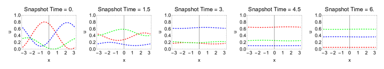
We now illustrate this for , and , and simultaneously show the existence of the predicted limit cycle solution for Eq. 16. Consider the following initial conditions for the PDE’s Eq. 8 and Eq. 9,
and assume periodic boundary conditions . Then four snapshots of the resulting travelling wave solution are shown in Fig. 1.
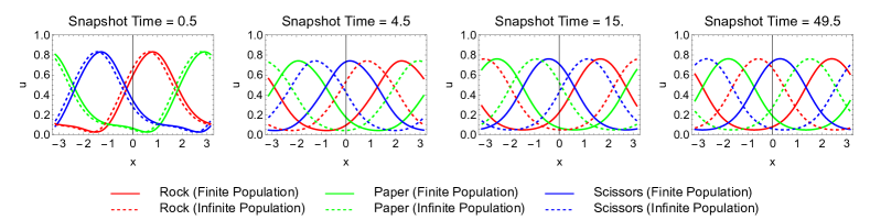
We see a perturbation of the initial condition that quickly settles into the travelling wave solution in both the finite and infinite population cases.
We can numerically investigate solutions for Eq. 16. Let be the (numerical) travelling wave solutions to the infinite (finite) population spatial replicator. For and in Eq. 16, we set,
where is sufficiently large to ensure that the resulting numeric solution is (effectively) on the limit cycle. When we plot for (in an appropriate projection) we see that the solutions to the partial differential equation(s) approach the limit cycle, as expected. This is shown in Fig. 2
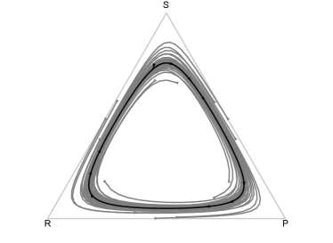
Recall that when , the interior fixed point () in the aspatial dynamics is unstable. We conclude that the travelling wave solution arises because the diffusion is stabilising the growing oscillations that would arise at all points in space and (under certain initial conditions), allowing the stabilised oscillations to synchronize.
We can prove this stabilisation occurs by first order analysis of the infinite population system. Let be the Jacobian of the equation system given in Eqs. 10 to 12 evaluated at the interior fixed point. Then we have,
| (19) |
Let with and let , where is the identify matrix. Following [72], we analyse the linearised stationary problem with Neumann boundary conditions,
by computing the roots of the characteristic polynomial,
Here is a wave number in a Fourier basis of a proposed solution ansatz and is an eigenvalue. We find three eigenvalues,
The fact that appears in the real parts of all three eigenvalues is sufficient to show that the diffusion exerts only a stabilising effect. Moreover,
is positive only if . That is , which we already knew. Thus, we have not only shown that the diffusion exerts a stabilising effect on the system, but also that Turing patterns cannot emerge in this system as a result of diffusion induced instability. Interestingly, this seems also explain the occurrence of travelling waves when no higher order interactions are present but in the interaction matrix in Eq. 4 using the infinite population spatial replicator as shown in [49]. We discuss this as a possible framework for generalising these results in future directions.
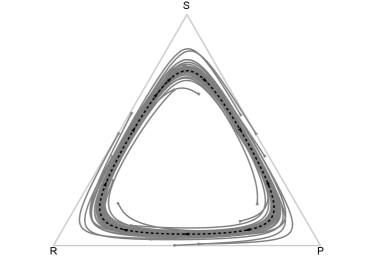
While it is generally difficult to construct the amplitude of a limit cycle, and thus a travelling wave, we can show numerically that the amplitude of the travelling wave (limit cycle) varies inversely with (a function of) the diffusion constant. Thus, as increases, we expect to see travelling wave solutions that approach the fixed point solution , further demonstrating the stabilising effect of the diffusion. This is illustrated in Fig. 3 for in the infinite population case.
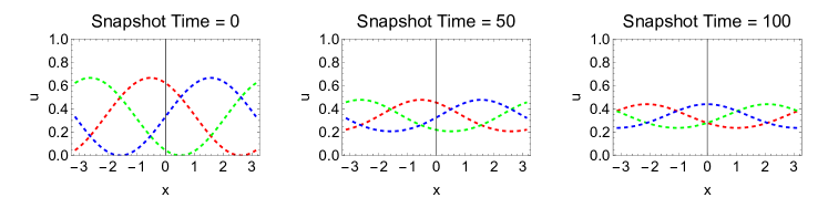
We can prove, by counter-example, that the travelling wave solution is not globally asymptotically stable in the space of solutions for either the finite population equation or the infinite population equation. To see this, consider the initial condition,
These expressions do not lead to (numerical) solutions that tend to travelling waves, as shown in Fig. 4.
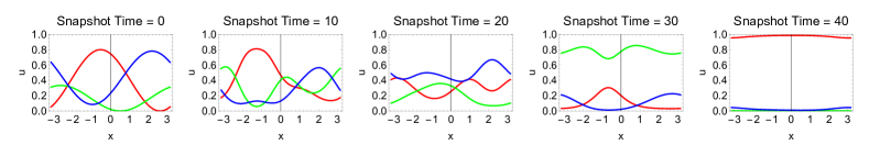
Instead, these solutions lead to a globally oscillating solution that asymptotically approaches the boundary of the simplex at all spatial positions. For the finite population case, we are using the travelling wave solution used in our prior numerical illustration. Interestingly, the finite population case takes longer to approach the globally oscillating solution than the infinite population case, most likely as a result of the bulk movement of the finite population. This is illustrated in Fig. 4(bottom). This phenomenon may warrant investigation in future work.
V Generalisation
To generalise the work in this paper, recall that a circulant matrix [73] has structure,
That is, the entire matrix structure is determined by the first row. The set of all circulant matrices forms an algebra under addition and (commutative) matrix multiplication.
Let with . Consider the dimensional row vector,
where is the biasing term. Then the circulant matrix defined by is the payoff matrix for the strategy generalisation of rock-paper-scissors. Griffin and Fan [74] showed that the replicator dynamics Eq. 1 have a unique interior fixed point at that is stable when and unstable when . Then we have the following conjecture, which is proved for the case .
Conjecture 1.
For all odd , the one-dimensional spatial replicator equation,
admits a travelling wave solution when is defined as above and .
We hypothesize that As in the three strategy case (rock-paper-scissors), when , , which implies a globally decreasing population.
Generalising our result to the higher order interaction case produces a surprising result. To generalise the interaction tensor to the case of strategies, let be the strategy set and let denote the set of strategies that are beaten by strategy and let be the set of strategies that beat strategy . Then,
| (20) |
The last three cases produce the diagonals and the case when the three strategies form a winning/losing cycle (like rock, paper and scissors). As before, . When , we recover the higher order interaction matrices we have already studied.
Consider . Then evaluating at and gives,
This value is if and only if and otherwise its sign is equivalent to . Notice, the triples are composed of entries of the form where and therefore cannot occur in the case when , which is why in our prior analysis. Simple computation shows that the only way for to be zero is in the case when . Further analysis shows that the eigenvalues of the Jacobian at the (unique) interior fixed point () are,
| (21) | |||
| (22) | |||
| (23) |
Thus the interior fixed point is unstable just in case , as in the three strategy case, which we conjecture will lead to a stable travelling wave solution in the infinite population spatial case. We summarize this in the following conjecture.
Conjecture 2.
For all odd , the one-dimensional higher order spatial replicator equation,
admits a travelling wave solution when and () are defined as above and , and and .
We note that the computation of the first Lyapunov coefficient will most likely be the most difficult component of any proofs of the generalised conjectures.
What is perhaps the most interesting aspect of this is the fact that higher order interactions as defined by Eq. 20 seem to be able to simultaneously produce travelling wave solutions and maintain a constant population size only for the three strategy rock-paper-scissors game. While we do not rule out the possibility that a more complex interaction mechanism may be able to simultaneously accomplish this, it is surprising that this property seems to hold for only the three strategy case and thus may warrant additional study.
VI Conclusions and Future Directions
In this paper, we merged the higher order interaction model first discussed by Griffin and Wu [29] with the spatial replicator equation model of Vickers [43] and the finite population spatial model of Griffin, Mummah and Deforest [49]. For higher order interactions in rock-paper-scissors, we showed that travelling wave solutions exist in both the finite and infinite population cases, with the important model feature that the net population was stable (as opposed to declining). This suggests that if replicators are models of real-world cyclically interacting populations, then travelling waves in such populations can be explained by either a declining population count or the presence of higher order (i.e., non-pairwise) interactions. In discussing a generalisation of this approach, we provided two conjectures on the existence of travelling wave solutions in spatial replicator dynamics with an arbitrary odd number of strategies. Most interestingly, we found that the property of population size preservation and the existence of travelling wave solutions appears to be present only in the rock-paper-scissors game (three strategy case), with higher order interactions. Games with more than three strategies (e.g., rock-paper-scissors-Spock-lizard) seem to admit travelling wave solutions only when the total population is decreasing and higher order interactions cannot remediate this.
Proving the conjectures raised in this paper is clearly an area of future work. We argue that stable Turing patterns will not be admitted by the infinite population spatial replicator with higher order interactions as defined in this paper. However, Griffin and Wu [29] show that a (subcritical) Hopf bifurcation can emerge in the aspatial higher order dynamics using a related but distinct payoff matrix and higher order interaction matrices. If parameter regimes exist where a supercritical Hopf bifurcation exists in the aspatial case, then it may be possible that a diffusion mediated transition maybe possible from periodic solutions to asymptotically stable solutions as in the work of Ginzburg and Landau equation [75] or in the work of Dilão [76]. Investigating this possibility of significant interest for future work.
Acknowledgements
C.G. was supported in part by the National Science Foundation under grant CMMI-1932991. C.G. would also like to thank Andrew Belmonte for a useful discussion on this topic.
Data and Code Availability
Three Mathematica notebooks are provided as supplementary materials and contain the code needed to reproduce the images and theoretical derivations in this paper.
Appendix A Constructing the First Lyapunov Coefficient
The approach outlined here is provided in [71] and is distilled from the detailed discussion in [70]. We begin by setting and , since we can see that . Then Eq. 16 reduces to four linearly independent equations. Let be the Jacobian of this reduced dimension system evaluated at the fixed point and and the special wave speed using the negative branch. Thus,
As expected, this matrix has two pure imaginary eigenvalues of form , where,
Let be the normalized eigenvector of so that and let be the normalized eigenvector of so that . The values of these eigenvectors can be computed in terms of , and as,
where
For simplicity of notation, write the reduced dimension version of Eq. 16 as,
where and for , is defined from Eq. 16. Let be the equilibrium point. Define componentwise as,
Define componentwise as,
Lastly, define the complex inner product,
where denotes the complex conjugate of the . Then is computed as,
Here, is an identity matrix of appropriate size. Using Mathematica (see SI), it is straightforward to compute that,
leaving only the term,
to be evaluated. A human assisted computation with Mathematica (see SI) yields the expression,
To prove this value is always negative, and thus that the limit cycle is always attracting, it suffices to show that,
for all allowable parameters. Computation is easier in terms of , and at this point. When we substitute in their definitions, we obtain the inequality,
We can rewrite this as,
which implies,
Solving the inequality for yields the requirement that,
| (24) |
We know by our assumptions that . Therefore, it suffices to show that the left-hand-side of the inequality is always less than zero. To prove this, note that for all we have,
Thus multiplying the left and right-hand sides of Eq. 24 yields,
Therefore, it follows that
and for all , and thus the limit cycle is always attracting.
References
- Allesina and Levine [2011] S. Allesina and J. M. Levine, A competitive network theory of species diversity, Proceedings of the National Academy of Sciences 108, 5638 (2011).
- Grilli et al. [2017] J. Grilli, G. Barabás, M. J. Michalska-Smith, and S. Allesina, Higher-order interactions stabilize dynamics in competitive network models, Nature 548, 210 (2017).
- Miller et al. [2023] Z. R. Miller, M. Clenet, K. D. Libera, F. Massol, and S. Allesina, Coexistence of many species under a random competition-colonization trade-off, bioRxiv 10.1101/2023.03.23.533867 (2023), https://www.biorxiv.org/content/early/2023/07/13/2023.03.23.533867.full.pdf .
- Paik and Griffin [2023] J. Paik and C. Griffin, Completely integrable replicator dynamics associated to competitive networks, Physical Review E 107, L052202 (2023).
- Itoh [1987] Y. Itoh, Integrals of a lotka-volterra system of odd number of variables, Progress of theoretical physics 78, 507 (1987).
- Veselov and Shabat [1993] A. P. Veselov and A. B. Shabat, Dressing chains and spectral theory of the schrodinger operator, Funktsional’nyi Analiz i ego Prilozheniya 27, 1 (1993).
- Bogoyavlensky [1988] O. Bogoyavlensky, Integrable discretizations of the kdv equation, Physics Letters A 134, 34 (1988).
- May [1972] R. M. May, Will a large complex system be stable?, Nature 238, 413 (1972).
- Pomerantz [1981] M. J. Pomerantz, Do” higher order interactions” in competition systems really exist?, The American Naturalist 117, 583 (1981).
- Relyea and Yurewicz [2002] R. A. Relyea and K. L. Yurewicz, Predicting community outcomes from pairwise interactions: integrating density-and trait-mediated effects, Oecologia 131, 569 (2002).
- Kodera et al. [2022] S. M. Kodera, P. Das, J. A. Gilbert, and H. L. Lutz, Conceptual strategies for characterizing interactions in microbial communities, Iscience , 103775 (2022).
- Levine et al. [2017] J. M. Levine, J. Bascompte, P. B. Adler, and S. Allesina, Beyond pairwise mechanisms of species coexistence in complex communities, Nature 546, 56 (2017).
- Bairey et al. [2016] E. Bairey, E. D. Kelsic, and R. Kishony, High-order species interactions shape ecosystem diversity, Nature communications 7, 1 (2016).
- McClean et al. [2019] D. McClean, V.-P. Friman, A. Finn, L. I. Salzberg, and I. Donohue, Coping with multiple enemies: pairwise interactions do not predict evolutionary change in complex multitrophic communities, Oikos 128, 1588 (2019).
- Skardal et al. [2021] P. S. Skardal, L. Arola-Fernández, D. Taylor, and A. Arenas, Higher-order interactions can better optimize network synchronization, Physical Review Research 3, 043193 (2021).
- Kleinhesselink et al. [2022] A. R. Kleinhesselink, N. J. Kraft, S. W. Pacala, and J. M. Levine, Detecting and interpreting higher-order interactions in ecological communities, Ecology letters 25, 1604 (2022).
- Gibbs et al. [2022] T. Gibbs, S. A. Levin, and J. M. Levine, Coexistence in diverse communities with higher-order interactions, Proceedings of the National Academy of Sciences 119, e2205063119 (2022), https://www.pnas.org/doi/pdf/10.1073/pnas.2205063119 .
- Battiston et al. [2021] F. Battiston, E. Amico, A. Barrat, G. Bianconi, G. Ferraz de Arruda, B. Franceschiello, I. Iacopini, S. Kéfi, V. Latora, Y. Moreno, et al., The physics of higher-order interactions in complex systems, Nature Physics 17, 1093 (2021).
- Battiston et al. [2020] F. Battiston, G. Cencetti, I. Iacopini, V. Latora, M. Lucas, A. Patania, J.-G. Young, and G. Petri, Networks beyond pairwise interactions: structure and dynamics, Physics Reports 874, 1 (2020).
- Lambiotte et al. [2019] R. Lambiotte, M. Rosvall, and I. Scholtes, From networks to optimal higher-order models of complex systems, Nature physics 15, 313 (2019).
- Swain et al. [2022] A. Swain, L. Fussell, and W. F. Fagan, Higher-order effects, continuous species interactions, and trait evolution shape microbial spatial dynamics, Proceedings of the National Academy of Sciences 119, e2020956119 (2022).
- Mayfield and Stouffer [2017] M. M. Mayfield and D. B. Stouffer, Higher-order interactions capture unexplained complexity in diverse communities, Nature ecology & evolution 1, 1 (2017).
- Mickalide and Kuehn [2019] H. Mickalide and S. Kuehn, Higher-order interaction between species inhibits bacterial invasion of a phototroph-predator microbial community, Cell Systems 9, 521 (2019).
- Deng et al. [2022] J. Deng, W. Taylor, and S. Saavedra, Understanding the impact of third-party species on pairwise coexistence, PLOS Computational Biology 18, e1010630 (2022).
- Weibull [1997] J. W. Weibull, Evolutionary Game Theory (MIT Press, 1997).
- Hofbauer and Sigmund [1998] J. Hofbauer and K. Sigmund, Evolutionary Games and Population Dynamics (Cambridge University Press, 1998).
- Hofbauer and Sigmund [2003] J. Hofbauer and K. Sigmund, Evolutionary Game Dynamics, Bulletin of the American Mathematical Society 40, 479 (2003).
- Friedman and Sinervo [2016] D. Friedman and B. Sinervo, Evolutionary games in natural, social, and virtual worlds (Oxford University Press, 2016).
- Griffin and Wu [2023] C. Griffin and R. Wu, Higher-order dynamics in the replicator equation produce a limit cycle in rock-paper-scissors, Europhysics Letters 142, 33001 (2023).
- Zeeman [1980] E. C. Zeeman, Population dynamics from game theory, in Global Theory of Dynamical Systems, Springer Lecture Notes in Mathematics No. 819 (Springer, 1980) pp. 471–497.
- Gokhale and Traulsen [2010] C. S. Gokhale and A. Traulsen, Evolutionary games in the multiverse, Proceedings of the National Academy of Sciences 107, 5500 (2010).
- Zhang et al. [2022] X. Zhang, P. Peng, Y. Zhou, H. Wang, and W. Li, Evolutionary game-theoretical analysis for general multiplayer asymmetric games, arXiv preprint arXiv:2206.11114 (2022).
- Peixe and Rodrigues [2022] T. Peixe and A. Rodrigues, Persistent strange attractors in 3d polymatrix replicators, Physica D: Nonlinear Phenomena 438, 133346 (2022).
- Alishah and Duarte [2015] H. N. Alishah and P. Duarte, Hamiltonian evolutionary games, Journal of Dynamics and Games 2, 33 (2015).
- Paulson and Griffin [2016] E. Paulson and C. Griffin, Cooperation can emerge in prisoner’s dilemma from a multi-species predator prey replicator dynamic, Mathematical biosciences 278, 56 (2016).
- Cressman and Vickers [1997] R. Cressman and G. Vickers, Spatial and density effects in evolutionary game theory, Journal of theoretical biology 184, 359 (1997).
- deForest and Belmonte [2013] R. deForest and A. Belmonte, Spatial pattern dynamics due to the fitness gradient flux in evolutionary games, Physical Review E 87 (2013).
- Kerr et al. [2002] B. Kerr, M. Riley, M. Feldman, and B. BJM, Local dispersal promotes biodiversity in a real-life game of rock–paper–scissors, Nature 418.6894, 171 (2002).
- Nowak and May [1992] M. Nowak and R. May, Evolutionary games and spatial chaos, Nature 359.6398, 826 (1992).
- Roca et al. [2009] C. Roca, J. Cuesta, and A. Sánchez, Evolutionary game theory: Temporal and spatial effects beyond replicator dynamics, Physics of life reviews 6.4, 208 (2009).
- Szabó et al. [2004] G. Szabó, A. Szolnoki, and R. Izsák, Rock-scissors-paper game on regular small-world networks, Journal of physics A: Mathematical and General 37.7, 2599 (2004).
- Vickers [1989] G. Vickers, Spatial patterns and ESS’s, Journal of Theoretical Biology 140, 129 (1989).
- Vickers [1991] G. Vickers, Spatial patterns and travelling waves in population genetics, Journal of Theoretical Biology 150, 329 (1991).
- He et al. [2010] Q. He, M. Mobilia, and U. C. Täuber, Spatial rock-paper-scissors models with inhomogeneous reaction rates, Physical Review E 82, 051909 (2010).
- Szczesny et al. [2014] B. Szczesny, M. Mobilia, and A. M. Rucklidge, Characterization of spiraling patterns in spatial rock-paper-scissors games, Physical Review E 90, 032704 (2014).
- Postlethwaite and Rucklidge [2017] C. Postlethwaite and A. Rucklidge, Spirals and heteroclinic cycles in a spatially extended rock-paper-scissors model of cyclic dominance, EPL (Europhysics Letters) 117, 48006 (2017).
- Postlethwaite and Rucklidge [2019] C. M. Postlethwaite and A. M. Rucklidge, A trio of heteroclinic bifurcations arising from a model of spatially-extended rock–paper–scissors, Nonlinearity 32, 1375 (2019).
- Durrett and Levin [1994] R. Durrett and S. Levin, The Importance of Being Discrete (and Spatial), Theoretical Population Biology 46, 363 (1994).
- Griffin et al. [2021] C. Griffin, R. Mummah, and R. deForest, A finite population destroys a traveling wave in spatial replicator dynamics, Chaos, Solitons & Fractals 146, 110847 (2021).
- Griffin [2023] C. Griffin, On a finite population variation of the fisher–kpp equation, Communications in Nonlinear Science and Numerical Simulation , 107369 (2023).
- Fort [2008] H. Fort, On evolutionary spatial heterogeneous games, Physica A: Statistical Mechanics and its Applications 387, 1613 (2008).
- Killingback and Doebeli [1996] T. Killingback and M. Doebeli, Spatial evolutionary game theory: Hawks and doves revisited, Proceedings of the Royal Society of London. Series B: Biological Sciences 263, 1135 (1996).
- Miekisz [2004] J. Miekisz, Statistical mechanics of spatial evolutionary games, Journal of Physics A: Mathematical and General 37, 9891 (2004).
- Nowak et al. [1994] M. A. Nowak, S. Bonhoeffer, and R. M. May, More spatial games, International Journal of Bifurcation and Chaos 4, 33 (1994).
- Ohtsuki and Nowak [2006] H. Ohtsuki and M. A. Nowak, Evolutionary games on cycles, Proceedings of the Royal Society B: Biological Sciences 273, 2249 (2006).
- Perc [2006] M. Perc, Chaos promotes cooperation in the spatial prisoner’s dilemma game, Europhysics Letters 75, 841 (2006).
- Szabó and Hódsági [2016] G. Szabó and K. Hódsági, The role of mixed strategies in spatial evolutionary games, Physica A: Statistical Mechanics and its Applications 462, 198 (2016).
- Wakano and Hauert [2011] J. Y. Wakano and C. Hauert, Pattern formation and chaos in spatial ecological public goodsgames, Journal of theoretical biology 268, 30 (2011).
- May [1994] R. M. May, Spatial chaos and its role in ecology and evolution, in Frontiers in mathematical Biology (Springer, 1994) pp. 326–344.
- Hutson and Vickers [1992] V. Hutson and G. T. Vickers, Travelling waves and dominance of ess’s, Journal of Mathematical Biology 30, 457 (1992).
- Vickers et al. [1993] G. Vickers, V. Hutson, and C. J. Budd, Spatial patterns in population conflicts, Journal of Mathematical Biology 31, 411 (1993).
- Hutson and Vickers [1995] V. Hutson and G. Vickers, The spatial struggle of tit-for-tat and defect, Philosophical Transactions of the Royal Society of London. Series B: Biological Sciences 348, 393 (1995).
- Bratus et al. [2011] A. S. Bratus, V. P. Posvyanskii, and A. S. Novozhilov, A note on the replicator equation with explicit space and global regulation, Mathematical Biosciences and Engineering 8, 659 (2011).
- Novozhilov et al. [2012] A. S. Novozhilov, V. P. Posvyanskii, and A. S. Bratus, On the reaction–diffusion replicator systems: spatial patterns and asymptotic behaviour, Russian Journal of Numerical Analysis and Mathematical Modelling 26, 555 (2012).
- Berthier et al. [2014] K. Berthier, S. Piry, J.-F. Cosson, P. Giraudoux, J.-C. Foltête, R. Defaut, D. Truchetet, and X. Lambin, Dispersal, landscape and travelling waves in cyclic vole populations, Ecology letters 17, 53 (2014).
- Kaitala [2002] V. Kaitala, Travelling waves in spatial population dynamics, in Annales Zoologici Fennici (JSTOR, 2002) pp. 161–171.
- Kot [1992] M. Kot, Discrete-time travelling waves: ecological examples, Journal of mathematical biology 30, 413 (1992).
- Sherratt and Smith [2008] J. A. Sherratt and M. J. Smith, Periodic travelling waves in cyclic populations: field studies and reaction–diffusion models, Journal of the Royal Society Interface 5, 483 (2008).
- Guckenheimer and Holmes [2013] J. Guckenheimer and P. Holmes, Nonlinear oscillations, dynamical systems, and bifurcations of vector fields, Vol. 42 (Springer Science & Business Media, 2013).
- Kuznetsov et al. [1998] Y. A. Kuznetsov, I. A. Kuznetsov, and Y. Kuznetsov, Elements of applied bifurcation theory, Vol. 112 (Springer, 1998).
- Pais et al. [2012] D. Pais, C. H. Caicedo-Nunez, and N. E. Leonard, Hopf bifurcations and limit cycles in evolutionary network dynamics, SIAM Journal on Applied Dynamical Systems 11, 1754 (2012).
- Murray and Murray [2003] J. D. Murray and J. D. Murray, Mathematical Biology: II: Spatial Models and Biomedical Applications, Vol. 3 (Springer, 2003).
- Davis [2012] P. J. Davis, Circulant Matrices, 2nd ed. (American Mathematical Society, 2012).
- Griffin and Fan [2022] C. Griffin and J. Fan, Control problems with vanishing lie bracket arising from complete odd circulant evolutionary games, Journal of Dynamics & Games (2022).
- Gambino et al. [2013] G. Gambino, M. Lombardo, M. Sammartino, and V. Sciacca, Turing pattern formation in the brusselator system with nonlinear diffusion, Physical Review E 88, 042925 (2013).
- Dilão [2005] R. Dilão, Turing instabilities and patterns near a hopf bifurcation, Applied mathematics and computation 164, 391 (2005).