Masses of the magnetized pseudoscalar and vector mesons in an extended NJL model: the role of axial vector mesons

Abstract

We study the mass spectrum of light pseudoscalar and vector mesons in the presence of an external uniform magnetic field $\vec{B}$, considering the effects of the mixing with the axial vector meson sector. The analysis is performed within a two-flavor NJL-like model which includes isoscalar and isovector couplings together with a flavor mixing ’t Hooft-like term. The effect of the magnetic field on charged particles is taken into account by retaining the Schwinger phases carried by quark propagators, and expanding the corresponding meson fields in proper Ritus-like bases. The spin-isospin and spin-flavor decomposition of meson mass states is also analyzed. For neutral pion masses it is shown that the mixing with axial vector mesons improves previous theoretical results, leading to a monotonic decreasing behavior with $B$ that is in good qualitative agreement with LQCD calculations, both for the case of constant or $B$-dependent couplings. Regarding charged pions, it is seen that the mixing softens the enhancement of their mass with $B$. As a consequence, the energy becomes lower than the one corresponding to a pointlike pion, improving the agreement with LQCD results. The agreement is also improved for the magnetic behavior of the lowest $\rho^{+}$ energy state, which does not vanish for the considered range of values of $B$ — a fact that can be relevant in connection with the occurrence of meson condensation for strong magnetic fields.

I Introduction

The effects caused by magnetic fields larger than $|eB|\sim\Lambda_{QCD}^{2}$ on the properties of strong-interacting matter have attracted a lot of attention along the last decades [2, 3, 4]. In part, this is motivated by the realization that such magnetic fields might play an important role in the study of the early Universe [5, 6], in the analysis of high energy noncentral heavy ion collisions [7, 8] and in the description of compact stellar objects like the magnetars [9, 10]. In addition to this phenomenological relevance, from the theoretical point of view, external magnetic fields can be used to probe QCD dynamics, allowing for a confrontation of theoretical results obtained through different approaches to nonperturbative QCD. In this sense, several interesting phenomena have been predicted to be induced by the presence of strong magnetic fields. They include the chiral magnetic effect [11, 12, 13], the enhancement of the QCD quark-antiquark condensate (magnetic catalysis) [14], the decrease of critical temperatures for chiral restoration and deconfinement QCD transitions (inverse magnetic catalysis) [15, 16], etc.

In this context, the understanding of the way in which the properties of light hadrons are modified by the presence of an intense magnetic field becomes a very relevant task. Clearly, this is a nontrivial problem, since first-principle theoretical calculations require to deal in general with QCD in a low energy nonperturbative regime. As a consequence, the corresponding theoretical analyses have been carried out using a variety of approaches. The effect of intense external magnetic fields on $\pi$ meson properties has been studied e.g. in the framework of Nambu-Jona-Lasinio (NJL)-like models [17, 18, 19, 20, 21, 22, 23, 24, 25, 26, 27, 28, 29, 30, 31, 32, 33, 34, 35, 36], quark-meson models [37, 38, 39, 40, 41], chiral perturbation theory (ChPT) [43, 42, 44], path integral Hamiltonians [45, 46], effective chiral confinement Lagrangians [47, 48] and QCD sum rules [49]. In addition, several results for the $\pi$ meson spectrum in the presence of background magnetic fields have been obtained from lattice QCD (LQCD) calculations [15, 51, 50, 52, 53, 54]. Regarding the $\rho$ meson sector, studies of magnetized $\rho$ meson masses in the framework of effective models and LQCD can be found in Refs. [35, 56, 46, 21, 26, 31, 55, 58, 57, 59] and Refs. [61, 51, 60, 50, 62, 52], respectively. The effect of an external magnetic field on nucleon masses has also been considered in several works [63, 64, 65, 66, 67, 68, 69, 70, 71].

In most of the existing model calculations of meson masses the mixing between states of different spin/isospin has been neglected. Although such mixing contributions are usually forbidden by isospin and/or angular momentum conservation, they can be nonzero (and may become important) in the presence of the external magnetic field. Effects of this kind have been studied recently by some of the authors of the present work, for both neutral [72] and charged mesons [73]. Those analyses have been performed in the framework of an extended NJL-like model, where, for simplicity, possible axial vector interactions have been neglected. The aim of the present work is to study how those previous results get modified when the presence of axial vector mesons is explicitly taken into account. In fact, due to symmetry reasons, in the context of the NJL model and its extensions [74, 75, 76] vector and axial vector interactions are expected to be considered on the same footing (see e.g. Refs. [77, 78]). This, in turn, implies the existence of the so-called “$\pi$-a₁ mixing” even at vanishing external magnetic field. Such a mixing has to be properly taken into account in order to correctly identify the pion mass states. Thus, the inclusion of the axial interactions is expected to be particularly relevant for the analysis of lowest meson masses.

Regarding the explicit calculation, as shown in previous works [27, 30, 73, 79, 80], one has to deal with the meson wavefunctions that arise as solutions of the equations of motion in the presence of the external magnetic field (which we assume to be static and uniform). In particular, in the case of charged mesons, it is seen that one-loop level calculations involve the presence of Schwinger phases that induce a breakdown of translational invariance in quark propagators [81]. As a consequence, the corresponding meson polarization functions are not diagonal for the standard plane wave states; one should describe meson states in terms of wavefunctions characterized by a set of quantum numbers that include the Landau level $\ell$. In addition, it is important to care about the regularization of ultraviolet divergences, since the presence of the external magnetic field can lead to spurious results, such as unphysical oscillations of physical observables [82, 83]. As in previous works [72, 73], we use the so-called magnetic field independent regularization (MFIR) scheme [84, 20, 22, 27], which has been shown to be free from these oscillations; moreover, it is seen that within this scheme the results are less dependent on model parameters [83]. Concerning the effective coupling constants of the model, we consider both the case in which these parameters are kept constant and the case in which they show some explicit dependence on the external magnetic field. This last possibility, inspired by the magnetic screening of the strong coupling constant occurring for a large magnetic field [85], has been previously explored in effective models [86, 87, 88, 70, 33] in order to reproduce the inverse magnetic catalysis effect observed at finite temperature LQCD calculations.

The paper is organized as follows. In Sec. II we introduce the magnetized extended NJL-like lagrangian to be used in our calculations, as well as the expressions of the relevant mean field quantities to be evaluated, such as quark masses and chiral condensates. In Sec. III and IV we present the formalisms used to obtain neutral and charged meson masses, respectively, in the presence the magnetic field. In Sec. V we present and discuss our numerical results, while in Sec. VI we provide a summary of our work, together with our main conclusions. We also include several appendices to provide some technical details of our calculations.

II Effective Lagrangian and mean field quantities

Let us start by considering the Lagrangian density for an extended NJL two-flavor model in the presence of an electromagnetic field. We have, in Minkowski space,

$${\cal L} = \bar{\psi}(x)\left(i\,\hbox to0.0pt{/\hss}\!D-m_{c}\right)\psi(x)+g_{S}\sum_{a=0}^{3}\Big{[}\left(\bar{\psi}(x){\tau_{b}}\psi(x)\right)^{2}+\left(\bar{\psi}(x)\,i\gamma_{5}{\tau_{b}}\psi(x)\right)^{2}\Big{]}$$ (1)

$$-\,g_{V}\left[\left(\bar{\psi}(x)\,\gamma_{\mu}\vec{\tau}\,\psi(x)\right)^{2}+\left(\bar{\psi}(x)\,\gamma_{\mu}\,\gamma_{5}\,\vec{\tau}\,\psi(x)\right)^{2}\right]$$

$$-\,g_{V_{0}}\left(\bar{\psi}(x)\,\gamma_{\mu}\,\psi(x)\right)^{2}-\,g_{A_{0}}\left(\bar{\psi}(x)\,\gamma_{\mu}\,\gamma_{5}\,\psi(x)\right)^{2}+\,2g_{D}\,\left(d_{+}+d_{-}\right)\ ,$$

where $\psi=(u\ d)^{T}$, ${\tau_{b}}=(\mathbbm{1},\vec{\tau})$, $\vec{\tau}$ being the usual Pauli-matrix vector, and $m_{c}$ is the current quark mass, which is assumed to be equal for $u$ and $d$ quarks. The model includes isoscalar/isovector vector and axial vector couplings, as well as a ’t Hooft-like flavor-mixing term, where we have defined $d_{\pm}={\rm det}[\bar{\psi}(x)(1\pm\gamma_{5})\psi(x)]$. The interaction between the fermions and the electromagnetic field ${\cal A}_{\mu}$ is driven by the covariant derivative

$$D_{\mu}\ =\ \partial_{\mu}+i\,\hat{Q}\mathcal{A}_{\mu}\ ,$$ (2)

where $\hat{Q}=\mbox{diag}(Q_{u},Q_{d})$, with $Q_{u}=2e/3$ and $Q_{d}=-e/3$, $e$ being the proton electric charge. A summary of the notation and conventions used throughout this work can be found in App. A.

We consider here the particular case in which one has a homogenous stationary magnetic field $\vec{B}$ orientated along the axis 3, or $z$. Now, to write down the explicit form of $\mathcal{A}^{\mu}$ one has to choose a specific gauge. Some commonly used gauges are the symmetric gauge (SG) in which ${\cal A}^{\mu}(x)=(0,-B\,x^{2}/2,B\,x^{1}/2,0)$, the Landau gauge 1 (LG1) in which ${\cal A}^{\mu}(x)=\left(0,-B\,x^{2},0,0\right)$ and the Landau gauge 2 (LG2), in which ${\cal A}^{\mu}(x)=\left(0,0,B\,x^{1},0\right)$. In what follows we refer to them as “standard gauges”. To test the gauge independence of our results, all these gauges will be considered in our analysis.

Since we are interested in studying meson properties, it is convenient to bosonize the fermionic theory, introducing scalar, pseudoscalar, vector and axial vector fields ${\sigma_{b}}(x)$, ${\pi_{b}}(x)$, ${\rho_{b}^{\mu}}(x)$, ${a_{b}^{\mu}}$, with $b=0,1,2,3$, and integrating out the fermion fields. The bosonized action can be written as

$$S_{\mathrm{bos}} = -i\ln\det\!\big{(}i\mathcal{D}\big{)}-\frac{1}{4g}\int d^{4}x\ \Big{[}{\sigma_{0}}(x)\,{\sigma_{0}}(x)+\vec{\pi}(x)\cdot\vec{\pi}(x)\Big{]}$$ (3)

$$-\,\frac{1}{4g(1-2\alpha)}\int d^{4}x\ \Big{[}\vec{\sigma}(x)\cdot\vec{\sigma}(x)+{\pi_{0}}(x)\,{\pi_{0}}(x)\Big{]}$$

$$+\,\frac{1}{4g_{V}}\int d^{4}x\ \left[\vec{\rho}_{\mu}(x)\cdot\vec{\rho}^{\,\mu}(x)+\vec{a}_{\mu}(x)\cdot\vec{a}^{\,\mu}(x)\right]$$

$$+\frac{1}{4g_{V_{0}}}\int d^{4}x\ {\rho_{0\mu}}(x)\,{\rho_{0}^{\mu}}(x)+\frac{1}{4g_{A_{0}}}\int d^{4}x\ {a_{0\mu}}(x)\,{a_{0}^{\mu}}(x)\ ,$$

with

$$i\mathcal{D}_{x,x^{\prime}}\ =\ \delta^{(4)}(x-x^{\prime})\,\big{[}i\,\hbox to0.0pt{/\hss}\!D-m_{0}-{\tau_{b}}\left({\sigma_{b}}(x)+i\,\gamma_{5}\,{\pi_{b}}(x)+\gamma_{\mu}\,{\rho_{b}^{\mu}}(x)+\gamma_{\mu}\gamma_{5}\,{a_{b}^{\mu}}(x)\right)\big{]}\ ,$$ (4)

where a direct product to an identity matrix in color space is understood. For convenience we have introduced the combinations

$$g=g_{S}+g_{D}\ ,\qquad\qquad\alpha=\frac{g_{D}}{g_{S}+g_{D}}\ ,$$ (5)

so that the flavor mixing in the scalar-pseudoscalar sector is regulated by the constant $\alpha$. For $\alpha=0$ quark flavors $u$ and $d$ get decoupled, while for $\alpha=0.5$ one has maximum flavor mixing, as in the case of the standard version of the NJL model.

We proceed by expanding the bosonized action in powers of the fluctuations of the bosonic fields around the corresponding mean field (MF) values. We assume that the fields $\sigma_{b}(x)$ have nontrivial translational invariant MF values given by $\tau_{b}\,\bar{\sigma}_{b}=\mbox{diag}(\bar{\sigma}_{u},\bar{\sigma}_{d})$, while vacuum expectation values of other bosonic fields are zero; thus, we write

$$\mathcal{D}_{x,x^{\prime}}\ =\ \mathcal{D}_{x,x^{\prime}}^{\mbox{\tiny MF}}+\delta\mathcal{D}_{x,x^{\prime}}\ .$$ (6)

The MF piece is diagonal in flavor space. One has

$$\mathcal{D}_{x,x^{\prime}}^{{\mbox{\tiny MF}}}\ =\ {\rm diag}\big{(}\mathcal{D}_{x,x^{\prime}}^{{\mbox{\tiny MF}},\,u}\,,\,\mathcal{D}_{x,x^{\prime}}^{{\mbox{\tiny MF}},\,d}\big{)}\ ,$$ (7)

where

$$\mathcal{D}_{x,x^{\prime}}^{{\mbox{\tiny MF}},\,f}\ =\ -i\,\delta^{(4)}(x-x^{\prime})\left(i\hbox to0.0pt{/\hss}\partial+Q_{f}\,B\,x^{1}\,\gamma^{2}-M_{f}\right)\ ,$$ (8)

with $f=u,d$. Here $M_{f}=m_{c}+\bar{\sigma}_{f}$ is the quark effective mass for each flavor $f$.

The MF action per unit volume is given by

$$\frac{S_{\mathrm{bos}}^{\mbox{\tiny MF}}}{V^{(4)}}\ =-\ \frac{(1-\alpha)(\bar{\sigma}_{u}^{2}+\bar{\sigma}_{d}^{2})-2\,\alpha\,\bar{\sigma}_{u}\bar{\sigma}_{d}}{8g(1-2\,\alpha)}-\frac{iN_{c}}{V^{(4)}}\sum_{f=u,d}\int d^{4}x\,d^{4}x^{\prime}\ {\rm tr}_{D}\,\ln\left(\mathcal{S}_{x,x^{\prime}}^{{\mbox{\tiny MF}},\,f}\right)^{-1}\ ,$$ (9)

where ${\rm tr}_{D}$ stands for the trace over Dirac space, and $\mathcal{S}_{x,x^{\prime}}^{{\mbox{\tiny MF}},\,f}=\big{(}i\mathcal{D}_{x,x^{\prime}}^{{\mbox{\tiny MF}},\,f}\big{)}^{-1}$ is the MF quark propagator in the presence of the magnetic field. Its explicit expression can be written as

$$\mathcal{S}_{x,y}^{{\mbox{\tiny MF}},\,f}=e^{i\Phi_{Q_{f}}(x,y)}\int\frac{d^{4}p}{(2\pi)^{4}}\ e^{-i\,p(x-y)}\,\bar{S}^{f}(p_{\parallel},p_{\perp})\ ,$$ (10)

where

$$\bar{S}^{f}(p_{\parallel},p_{\perp}) = -\,i\int_{0}^{\infty}d\sigma\ \exp\!\bigg{[}\!-i\sigma\Big{(}M_{f}^{2}-p_{\parallel}^{2}+\vec{p}_{\perp}^{\ 2}\,\dfrac{\tan(\sigma B_{f})}{\sigma B_{f}}-i\epsilon\Big{)}\bigg{]}$$ (11)

$$\times\left[\left(p_{\parallel}\cdot\gamma_{\parallel}+M_{f}\right)(1-s_{f}\,\gamma^{1}\gamma^{2}\tan(\sigma B_{f}))-\frac{\vec{p}_{\perp}\cdot\vec{\gamma}_{\perp}}{\cos^{2}(\sigma B_{f})}\right]\ ,$$

with $B_{f}=|BQ_{f}|$ and $s_{f}={\rm sign}(BQ_{f})$. Here we have defined the “parallel” and “perpendicular” four-vectors

$$p_{\parallel}^{\mu}=(p^{0},0,0,p^{3})\ ,\qquad\qquad p_{\perp}^{\mu}=(0,p^{1},p^{2},0)\ ,$$ (12)

and equivalent definitions have been used for $\gamma_{\parallel}$, $\gamma_{\perp}$. The function $\Phi_{Q}(x,y)$ in Eq. (10) is the so-called Schwinger phase, which is shown to be a gauge dependent quantity. For the standard gauges one has

SG: $$\Phi_{Q}(x,y)=-\frac{QB}{2}(x^{1}y^{2}-y^{1}x^{2})\ ,\hskip 42.67912pt$$

LG1: $$\Phi_{Q}(x,y)=-\frac{QB}{2}(x^{2}+x^{2})(x^{1}-y^{1})\ ,\hskip 42.67912pt$$

LG2: $$\Phi_{Q}(x,y)=\frac{QB}{2}(x^{1}+y^{1})(x^{2}-y^{2})\ .\hskip 42.67912pt$$ (13)

Let us consider the quark-antiquark condensates $\phi_{f}\equiv\langle\bar{\psi}_{f}\psi_{f}\rangle$. For each flavor $f=u,d$ we have

$$\phi_{f}=iN_{c}\int\frac{d^{4}p}{(2\pi)^{4}}\ {\rm tr}_{D}\,\bar{S}^{f}(p_{\parallel},p_{\perp})\ .$$ (14)

The integral in this expression is divergent and has to be properly regularized. As stated in the Introduction, we use here the magnetic field independent regularization (MFIR) scheme: for a given unregularized quantity, the corresponding (divergent) $B\to 0$ limit is subtracted and then it is added in a regularized form. Thus, the quantities can be separated into a (finite) “$B=0$” part and a “magnetic” piece. Notice that, in general, the “$B=0$” part still depends implicitly on $B$ (e.g. through the values of the dressed quark masses $M_{f}$); hence, it should not be confused with the value of the studied quantity at vanishing external field. To deal with the divergent “$B=0$” terms we use here a proper time (PT) regularization scheme. Thus, we obtain

$$\phi_{f}^{{\rm reg}}\ =\ \phi_{f}^{0,\,{\rm reg}}\,+\,\phi_{f}^{{\rm mag}}\ ,$$ (15)

where

$$\phi_{f}^{0,{\rm reg}}=-N_{c}\,M_{f}\,I_{1f}\ ,\qquad\qquad\phi_{f}^{{\rm mag}}=-N_{c}\,M_{f}\,I_{1f}^{{\rm mag}}\ .$$ (16)

The expression of $I_{1f}$ obtained from the PT regularization, $I_{1f}^{\rm reg}$, is given in Eq. (C.15) in App. C, while the “magnetic” piece $I_{1f}^{{\rm mag}}$ reads

$$I_{1f}^{{\rm mag}}=\dfrac{B_{f}}{2\pi^{2}}\left[\ln\Gamma(x_{f})-\left(x_{f}-\dfrac{1}{2}\right)\ln x_{f}+x_{f}-\dfrac{\ln{2\pi}}{2}\right]\,,$$ (17)

where $x_{f}=M_{f}^{2}/(2B_{f})$. The corresponding gap equations, obtained from $\partial S_{\mathrm{bos}}^{\mbox{\tiny MF}}/\partial\bar{\sigma}_{f}=0$, can be written as

$$M_{u} = m_{c}-4g\left[(1-\alpha)\,\phi_{u}^{{\rm reg}}+\alpha\,\phi_{d}^{{\rm reg}}\right]\ ,$$

$$M_{d} = m_{c}-4g\left[(1-\alpha)\,\phi_{d}^{{\rm reg}}+\alpha\,\phi_{u}^{{\rm reg}}\right]\ .$$ (18)

As anticipated, for $\alpha=0$ these equations get decoupled. For $\alpha=0.5$ the right hand sides become identical, thus one has in that case $M_{u}=M_{d}$.

III The neutral meson sector

To determine the meson masses we have to consider the terms in the bosonic action that are quadratic in meson fluctuations. As expected from charge conservation, it is easy to see that the terms corresponding to charged and neutral mesons decouple from each other. In this section we concentrate on the neutral meson sector; the charged meson sector will be considered in Sec. IV.

III.1 Neutral meson polarization functions

For notational convenience we will denote isospin states by $M={\sigma_{0}},{\pi_{0}},{\rho_{0}^{\mu}},{a_{0}^{\mu}},{\sigma_{3}},{\pi_{3}},{\rho_{3}^{\mu}},{a_{3}^{\mu}}$. Here, ${\sigma_{0}}$, ${\pi_{0}}$, ${\rho_{0}}$ and ${a_{0}}$ correspond to the isoscalar states $\sigma$, $\eta$, $\omega$ and $f_{1}$, while ${\sigma_{3}}$, ${\pi_{3}}$, ${\rho_{3}}$ and ${a_{3}}$ stand for the neutral components of the isovector triplets $\vec{\rm a}_{0}$, $\vec{\pi}$, $\vec{\rho}$ and $\vec{\rm a}_{1}$, respectively. Thus, the corresponding quadratic piece of the bosonized action can be written as

$$S_{\mathrm{bos}}^{{\rm quad,\,neutral}}\ =-\ \frac{1}{2}\int d^{4}x\;d^{4}x^{\prime}\sum_{M,M^{\prime}}\delta M(x)^{\dagger}\ {{\cal G}}_{MM^{\prime}}(x,x^{\prime})\ \delta M^{\prime}(x^{\prime})\ .$$ (19)

Notice that the meson indices $M,M^{\prime}$, as well as the functions ${{\cal G}}_{MM^{\prime}}$, include Lorentz indices in the case of vector mesons. This also holds for the functions $\delta_{MM^{\prime}}$, ${\cal J}_{MM^{\prime}}$, $\Sigma_{MM^{\prime}}^{f}$, $G_{MM^{\prime}}$, etc., introduced below. In the corresponding expressions, a contraction of Lorentz indices is understood when appropriate. In particular, the functions ${{\cal G}}_{MM^{\prime}}(x,x^{\prime})$ can be separated in two terms, namely

$${{\cal G}}_{MM^{\prime}}(x,x^{\prime})\ =\ \frac{1}{2g_{M}}\ \delta_{MM^{\prime}}\ \delta^{(4)}(x-x^{\prime})-\,{{\cal J}}_{MM^{\prime}}(x,x^{\prime})\ ,$$ (20)

where

$$\frac{1}{g_{M}}\ \delta_{MM^{\prime}}\ =\ \left\{\begin{array}[]{cl}1/g&\ \ \ \ \mbox{for}\ \ M=M^{\prime}={\sigma_{0}},{\pi_{3}}\\ 1/[g(1-2\alpha)]&\ \ \ \ \mbox{for}\ \ M=M^{\prime}={\sigma_{3}},{\pi_{0}}\\ -\eta^{\mu\nu}/g_{V}&\ \ \ \ \mbox{for}\ \ MM^{\prime}={\rho_{3}^{\mu}}{\rho_{3}^{\nu}},{a_{3}^{\mu}}{a_{3}^{\nu}}\\ -\eta^{\mu\nu}/g_{V_{0}}&\ \ \ \ \mbox{for}\ \ MM^{\prime}={\rho_{0}^{\mu}}{\rho_{0}^{\nu}}\\ -\eta^{\mu\nu}/g_{A_{0}}&\ \ \ \ \mbox{for}\ \ MM^{\prime}={a_{0}^{\mu}}{a_{0}^{\nu}}\end{array}\right.\qquad,$$ (21)

and $\delta_{MM^{\prime}}=0$ otherwise. Here $\eta^{\mu\nu}$ is the Minkowski metric tensor, which can be decomposed as $\eta^{\mu\nu}=\eta_{\parallel}^{\mu\nu}+\eta_{\perp}^{\mu\nu}$, with $\eta_{\parallel}^{\mu\nu}=\mbox{diag}(1,0,0,-1)$, $\eta_{\perp}^{\mu\nu}=\mbox{diag}(0,-1,-1,0)$ (see App. A). In turn, the polarization functions ${{\cal J}}_{MM^{\prime}}(x,x^{\prime})$ can be separated into $u$ and $d$ quark pieces,

$${{\cal J}}_{MM^{\prime}}(x,x^{\prime})\ =\ \mathit{\Sigma}_{MM^{\prime}}^{u}(x,x^{\prime})\,+\,\varepsilon_{M}\,\varepsilon_{M^{\prime}}\,\mathit{\Sigma}_{MM^{\prime}}^{d}(x,x^{\prime})\ .$$ (22)

Here $\varepsilon_{M}=1$ for the isoscalars $M={\sigma_{0}},{\pi_{0}},{\rho_{0}^{\mu}},{a_{0}^{\mu}}$ and $\varepsilon_{M}=-1$ for $M={\sigma_{3}},{\pi_{3}},{\rho_{3}^{\mu}},{a_{3}^{\mu}}$, while the functions $\mathit{\Sigma}_{MM^{\prime}}^{f}(x,x^{\prime})$ are given by

$$\mathit{\Sigma}_{MM^{\prime}}^{f}(x,x^{\prime})\ =-i\,N_{c}\ {\rm tr}_{D}\bigg{[}i\,\mathcal{S}_{x,x^{\prime}}^{{\mbox{\tiny MF}},\,f}\,\Gamma^{M^{\prime}}i\,\mathcal{S}_{x^{\prime},x}^{{\mbox{\tiny MF}},\,f}\,\Gamma^{M}\,\bigg{]}\ ,$$ (23)

with

$$\Gamma^{M}\ =\ \left\{\begin{array}[]{cl}\mathbbm{1}&\ \ \mbox{for}\ \ M={\sigma_{0}},{\sigma_{3}}\\ i\gamma_{5}&\ \ \mbox{for}\ \ M={\pi_{0}},{\pi_{3}}\\ \gamma^{\mu}&\ \ \mbox{for}\ \ M={\rho_{0}^{\mu}},{\rho_{3}^{\mu}}\\ \gamma^{\mu}\gamma_{5}&\ \ \mbox{for}\ \ M={a_{0}^{\mu}},{a_{3}^{\mu}}\end{array}\right.\qquad.$$ (24)

As stated, since we are dealing with neutral mesons, the contributions of Schwinger phases associated with the quark propagators in Eq. (10) cancel out, and the polarization functions depend only on the difference $x-x^{\prime}$, i.e., they are translationally invariant. After a Fourier transformation, the conservation of momentum implies that the polarization functions turn out to be diagonal in the momentum basis. Thus, in this basis the neutral meson contribution to the quadratic action can be written as

$$S_{\mathrm{bos}}^{{\rm quad,\,neutral}}\ =-\dfrac{1}{2}\sum_{M,M^{\prime}}\int\dfrac{d^{4}q}{(2\pi)^{4}}\ \delta M(-q)^{\dagger}\ {{G}}_{MM^{\prime}}(q)\ \delta M^{\prime}(q)\ .$$ (25)

We have

$${{G}}_{MM^{\prime}}(q)\ =\ \frac{1}{2g_{M}}\;\delta_{MM^{\prime}}\,-\,{{J}}_{MM^{\prime}}(q)\ ,$$ (26)

and the associated polarization functions can be written as

$${{J}}_{MM^{\prime}}(q)\ =\ \Sigma_{MM^{\prime}}^{u}(q)+\varepsilon_{M}\varepsilon_{M^{\prime}}\,\Sigma_{MM^{\prime}}^{d}(q)\ .$$ (27)

Here the functions $\Sigma_{MM^{\prime}}^{f}(q)$ read

$$\Sigma_{MM^{\prime}}^{f}(q)\ =-i\,N_{c}\,\int\frac{d^{4}p}{(2\pi)^{4}}\ {\rm tr}_{D}\left[i\,\bar{S}^{f}(p_{\parallel}^{+},p_{\perp}^{+})\,\Gamma^{M^{\prime}}i\,\bar{S}^{f}(p_{\parallel}^{-},p_{\perp}^{-})\,\Gamma^{M}\right]\ ,$$ (28)

where we have defined $p_{a}^{\pm}=p_{a}\pm q_{a}/2$, with $a=\parallel,\perp$, and the quark propagators $\bar{S}^{f}(p_{\parallel},p_{\perp})$ in the presence of the magnetic field are those given by Eq. (11). The explicit expressions of the non-vanishing functions $\Sigma_{MM^{\prime}}^{f}(q)$ for arbitrary four-momentum $q^{\mu}$ are given in App. B.

Since we are interested in the determination of meson masses, let us focus on the particular situation in which mesons are at rest, i.e. $q^{\mu}=(m,0,0,0)$, where $m$ is the corresponding meson mass. We denote by $\hat{J}_{MM^{\prime}}$ the resulting polarization functions. It can be shown that some of these functions vanish, while the nonvanishing ones are in general divergent. As we have done at the MF level, we consider the magnetic field independent regularization scheme, in which we subtract the corresponding unregularized “$B=0$” contributions and then we add them in a regularized form. Thus, for a given polarization function $\hat{{J}}_{MM^{\prime}}$ we have

$$\hat{{J}}_{MM^{\prime}}^{{\rm reg}}\ =\ \hat{{J}}_{MM^{\prime}}^{{0,{\rm reg}}}\,+\,\hat{{J}}_{MM^{\prime}}^{{\rm mag}}\ .$$ (29)

The “$B=0$” pieces of the polarization functions are quoted in App. C, considering arbitrary four-momentum $q^{\mu}$. In that appendix we give the expressions for the unregularized functions ${{J}}_{MM^{\prime}}^{0,{\rm unreg}}$, and use a proper time regularization scheme to get the regularized expressions ${{J}}_{MM^{\prime}}^{0,{\rm reg}}$. The terms $\hat{{J}}_{MM^{\prime}}^{{0,{\rm reg}}}$ in Eq. (29) are then obtained from these expressions by taking $q^{2}=m^{2}$. In the case of the “magnetic” contributions $\hat{{J}}_{MM^{\prime}}^{{\rm mag}}$, we proceed as follows: we take the full expressions for the polarization functions ${{J}}_{MM^{\prime}}(q)$ given in App. B, and subtract the unregularized pieces ${{J}}_{MM^{\prime}}^{0,{\rm unreg}}$; next, we take $q^{\mu}=(m,0,0,0)$ and make use of the relations in App. D, performing some integration by parts when convenient. After a rather long calculation, it is found that $\hat{{J}}_{MM^{\prime}}^{{\rm mag}}$ can be expressed in the form given by Eq. (27), viz.

$$\hat{{J}}_{MM^{\prime}}^{{\rm mag}}\ =\ \hat{\Sigma}_{MM^{\prime}}^{u,\,{\rm mag}}+\varepsilon_{M}\varepsilon_{M^{\prime}}\,\hat{\Sigma}_{MM^{\prime}}^{d,\,{\rm mag}}\ ,$$ (30)

where the functions $\hat{\Sigma}_{MM^{\prime}}^{f,\,{\rm mag}}$ are given by

$$\hat{\Sigma}_{\pi_{b}\pi_{b^{\prime}}}^{f,\,{\rm mag}} = N_{c}\,\Big{(}I_{1f}^{{\rm mag}}-m^{2}I_{2f}^{{\rm mag}}\Big{)}\ ,$$ (31)

$$\hat{\Sigma}_{\rho_{b}^{\mu}\rho_{b^{\prime}}^{\nu}}^{f,\,{\rm mag}\,\mu\nu} = N_{c}\,\Big{(}I_{4f}^{{\rm mag}}\,\eta_{\perp}^{\mu\nu}-m^{2}I_{5f}^{{\rm mag}}\,\delta_{\,3}^{\mu}\delta_{\,3}^{\nu}\Big{)}\ ,$$ (32)

$$\hat{\Sigma}_{a_{b}^{\mu}a_{b^{\prime}}^{\nu}}^{f,\,{\rm mag}\,\mu\nu} = -N_{c}\,\Big{[}4M_{f}^{2}I_{2f}^{{\rm mag}}\,\delta_{\,0}^{\mu}\delta_{\,0}^{\nu}\,-\left(I_{4f}^{{\rm mag}}+2M_{f}^{2}\,I_{7f}^{{\rm mag}}\right)\eta_{\perp}^{\mu\nu}$$ (33)

$$+\left(m^{2}I_{5f}^{{\rm mag}}-4M_{f}^{2}\,I_{2f}^{{\rm mag}}\right)\delta_{\,3}^{\mu}\delta_{\,3}^{\nu}\Big{]}\ ,$$

$$\hat{\Sigma}_{\pi_{b}\rho_{b^{\prime}}^{\mu}}^{f,\,{\rm mag}\,\mu} = -\hat{\Sigma}_{\rho_{b}^{\mu}\pi_{b^{\prime}}}^{f,\,{\rm mag}\,\mu}=-i\,s_{f}N_{c}\,I_{3f}^{{\rm mag}}\,\delta_{\,3}^{\mu}\ ,$$ (34)

$$\hat{\Sigma}_{\pi_{b}a_{b^{\prime}}^{\mu}}^{f,\,{\rm mag}\,\mu} = -\hat{\Sigma}_{a_{b}^{\mu}\pi_{b^{\prime}}}^{f,\,{\rm mag}\,\mu}=2i\,N_{c}\,m\,M_{f}\,I_{2f}^{{\rm mag}}\,\delta_{\,0}^{\mu}\ ,$$ (35)

$$\hat{\Sigma}_{a_{b}^{\mu}\rho_{b^{\prime}}^{\nu}}^{f,\,{\rm mag}\,\mu\nu} = \hat{\Sigma}_{\rho_{b}^{\nu}a_{b^{\prime}}^{\mu}}^{f,\,{\rm mag}\,\nu\mu}=s_{f}\,N_{c}\,\Big{[}\left(I_{6f}^{{\rm mag}}+M_{f}/m\,I_{3f}^{{\rm mag}}\right)\delta_{\,0}^{\mu}\delta_{\,3}^{\nu}$$ (36)

$$\qquad\qquad\quad+\left(I_{6f}^{{\rm mag}}-M_{f}/m\,I_{3f}^{{\rm mag}}\right)\delta_{\,3}^{\mu}\delta_{\,0}^{\nu}\Big{]}\ .$$

The expression for $I_{1f}^{{\rm mag}}$ has been given in Eq. (17), whereas the integrals $I_{nf}^{{\rm mag}}$ for $n=2,\dots,7$ read

$$I_{2f}^{{\rm mag}} = \frac{1}{8\pi^{2}}\int_{0}^{1}dv\left[\psi(\bar{x}_{f})+\frac{1}{2\bar{x}_{f}}-\ln\bar{x}_{f}\right]\ ,$$ (37)

$$I_{3f}^{{\rm mag}} = \frac{M_{f}m}{8\pi^{2}}\int_{0}^{1}dv\;\frac{1}{\bar{x}_{f}}\ ,$$ (38)

$$I_{4f}^{{\rm mag}} = -\,I_{1f}^{{\rm mag}}-\frac{B_{f}}{4\pi^{2}}\sum_{s=\pm 1}\int_{0}^{1}dv\ \bigg{(}\bar{x}_{f}+\frac{m^{2}}{4B_{f}}+\frac{sv}{2}\bigg{)}\Bigg{[}\ln\bar{x}_{f}-\psi\left(\bar{x}_{f}+\frac{1+sv}{2}\right)\Bigg{]}\ ,$$ (39)

$$I_{5f}^{{\rm mag}} = \frac{1}{8\pi^{2}}\int_{0}^{1}dv\ (1-v^{2})\left[\psi(\bar{x}_{f})+\frac{1}{2\bar{x}_{f}}-\ln\bar{x}_{f}\right]\ ,$$ (40)

$$I_{6f}^{{\rm mag}} = \frac{m^{2}}{32\pi^{2}}\int_{0}^{1}dv\;\frac{(1-v^{2})}{\bar{x}_{f}}\ ,$$ (41)

$$I_{7f}^{{\rm mag}} = \frac{1}{8\pi^{2}}\sum_{s=\pm 1}\int_{0}^{1}dv\ \Big{[}\ln\bar{x}_{f}-\psi\left(\bar{x}_{f}+\frac{1+sv}{2}\right)\Big{]}\ .$$ (42)

Here we have defined $\bar{x}_{f}=\left[M_{f}^{2}-(1-v^{2})m^{2}/4\right]/(2B_{f})$. For $m<2M_{f}$, the integrals in the above expressions are well defined, while for $m\geq 2M_{f}$ (i.e., beyond the $q\bar{q}$ production threshold) they are divergent. Still, if this is the case one can obtain finite results by performing analytic extensions [72].

III.2 Box structure of the neutral meson mass matrix

The quadratic piece of the bosonized action in Eq. (25) involves 20 meson states. However, it can be seen that some of these states do not get mixed, i.e., the $20\times 20$ mass matrix can be separated into several blocks, or “boxes”.

The vector fields ${\rho_{0}^{\mu}}$ and ${\rho_{3}^{\mu}}$, as well as the axial vector fields ${a_{0}^{\mu}}$ and ${a_{3}^{\mu}}$, can be written in a polarization vector basis. Since the magnetic field defines a privileged direction in space, to exploit the symmetries of the physical system it is convenient to choose one of the polarization vectors $\epsilon^{\mu}$ in such a way that the spatial part $\vec{\epsilon}\,$ is parallel to $\vec{B}$. A possible choice of a polarization vector set satisfying this condition is introduced in App. E: the polarization vector denoted by $\epsilon^{\mu}(\vec{q},2)$ is such that $\vec{\epsilon}\,(\vec{q},2)$ is parallel to the magnetic field, regardless of the three-momentum $\vec{q}$. Now, as explained in App. F, the system has an invariance related to the reflection on the plane perpendicular to the magnetic field axis. If we associate to this transformation an operator $\mathcal{P}_{3}$, the pseudoscalar and scalar particle states transform under $\mathcal{P}_{3}$ by getting phases $\eta_{\mathcal{P}_{3}}^{\pi_{b}}=-1$ and $\eta_{\mathcal{P}_{3}}^{\sigma_{b}}=1$, respectively (here $b=0,3$). In general, the transformation of the vector and axial vector states is more complicated, depending on their polarizations. However, the choice of $\epsilon^{\mu}(\vec{q},2)$ as one of the (orthogonal) polarization vectors guarantees a well definite behavior of vector particle states; indeed, considering the remaining polarization vectors in App. E, which are denoted by $\epsilon^{\mu}(\vec{q},c)$ with $c=1$, $3$, $L$, one has $\eta_{\mathcal{P}_{3}}^{\rho_{b,2}}=\eta_{\mathcal{P}_{3}}^{a_{b,1}}=\eta_{\mathcal{P}_{3}}^{a_{b,3}}=\eta_{\mathcal{P}_{3}}^{a_{b,L}}=-1$ and $\eta_{\mathcal{P}_{3}}^{a_{b,2}}=\eta_{\mathcal{P}_{3}}^{\rho_{b,1}}=\eta_{\mathcal{P}_{3}}^{\rho_{b,3}}=\eta_{\mathcal{P}_{3}}^{\rho_{b,L}}=1$. Here we have introduced the notation $\rho_{b,c}\,$, $a_{b,c}$, where $b=0$ and $b=3$ correspond to isoscalar an isovector states respectively, and the index $c$ ($=1,2,3,L$) indicates the polarization state.

To get rid of the Lorentz indices, it is convenient to deal with a mass matrix $\mathbf{G}$ in which the vector and axial vector meson entries are given by the corresponding projections onto the polarization vector states. Taking into account the matrix $G_{MM^{\prime}}$ in Eq. (25), and using the above mentioned polarization basis, we have

$${\mathbf{G}}_{s_{b}s^{\prime}_{b^{\prime}}} = {G}_{s_{b}s^{\prime}_{b^{\prime}}}\ ,$$

$${\mathbf{G}}_{s_{b}v_{b^{\prime}\!,c}} = {G}_{s_{b}v_{b^{\prime}}^{\mu}}^{\,\mu}\,\epsilon_{\mu}(\vec{q},c)\ ,$$

$${\mathbf{G}}_{v_{b,c}s_{b^{\prime}}} = \epsilon_{\mu}(\vec{q},c)^{\ast}\,{G}_{v_{b}^{\mu}s_{b^{\prime}}}^{\,\mu}\ ,$$

$${\mathbf{G}}_{v_{b,c}{v^{\prime}\!}_{b^{\prime}\!,c^{\prime}}} = \epsilon_{\mu}(\vec{q},c)^{\ast}\,{G}_{v_{b}^{\mu}{v^{\prime}}_{b^{\prime}}^{\nu}}^{\,\mu\nu}\,\epsilon_{\nu}(\vec{q},c^{\prime})\ ,$$ (43)

where $c,c^{\prime}=1,2,3,L$. Here $s$ and $s^{\prime}$ stand for the scalar or pseudoscalar states $\pi,\sigma$, while $v$ and $v^{\prime}$ stand for the vector or axial vector states $\rho,a$. Now, as shown in App. F, the fact that the system is invariant under the reflection in the plane perpendicular to the magnetic field implies that particles with different parity phases $\eta_{\mathcal{P}_{3}}^{M}$ cannot mix; therefore, the $20\times 20$ matrix $\mathbf{G}$ turns out to be separated into two $10\times 10$ blocks. It can be written as

$$\mathbf{G}\ =\ \mathbf{G}^{(-)}\oplus\,\mathbf{G}^{(+)}\ ,$$ (44)

where the corresponding meson subspaces are

$$\mathbf{G}^{(-)} ,\ {\rm states}\ \ \pi_{b},\ \rho_{b,2},\ a_{b,1},\ a_{b,3},\ a_{b,L}\ ,\quad b=0,3\ ;$$ (45)

$$\mathbf{G}^{(+)} ,\ {\rm states}\ \ \sigma_{b},\ \rho_{b,1},\ \rho_{b,3},\ \rho_{b,L},\ a_{b,2}\ ,\quad b=0,3\ .$$ (46)

There are more symmetry properties that can still be taken into account. Notice that, according to its definition, the polarization vector $\epsilon^{\mu}(\vec{q},2)$ is invariant under rotations around the axis 3, which implies that it is an eigenvector of the operator $S_{3}^{\mu\nu}=i\left(\delta_{1}^{\mu}\,\delta_{2}^{\nu}-\delta_{2}^{\mu}\,\delta_{1}^{\nu}\right)$ with eigenvalue $s_{3}=0$. Moreover, the whole physical system is invariant under rotations around the axis 3, and consequently the third component of total angular momentum, $J_{3}=\left(\vec{x}\times\vec{q}\right)_{3}+S_{3}$, has to be a good quantum number. Thus, if we let $\vec{q}_{\perp}=\vec{0}$, the quantum number $S_{3}$ will be a good one to characterize the meson states.

Let us consider the polarization vectors defined in App. E. As stated, $\epsilon^{\mu}(\vec{q},2)$ is an eigenvector of $S_{3}^{\mu\nu}$, while $\epsilon^{\mu}(\vec{q},L)$ is defined as a “longitudinal” vector, in the sense that its spatial part is parallel to $\vec{q}$. The remaining polarization vectors, $\epsilon^{\mu}(\vec{q},1)$ and $\epsilon^{\mu}(\vec{q},3)$, do not have in general a simple interpretation. Now, if we let $\vec{q}_{\perp}=0$, they reduce to

$$\epsilon^{\mu}(\vec{q}_{\parallel},1)=\frac{1}{\sqrt{2}}\left(0,1,i,0\right)\ ,\qquad\epsilon^{\mu}(\vec{q}_{\parallel},3)=\frac{1}{\sqrt{2}}\left(0,1,-i,0\right)\ ,$$ (47)

where $\vec{q}_{\parallel}=(0,0,q^{3})$. Thus, it is seen that $\vec{\epsilon}(\vec{q}_{\parallel},1)$ and $\vec{\epsilon}(\vec{q}_{\parallel},3)$ lie in the plane perpendicular to the magnetic field, and meson states with polarizations $\epsilon^{\mu}(\vec{q}_{\parallel},1)$ and $\epsilon^{\mu}(\vec{q}_{\parallel},3)$ are states of definite third component of the spin, with eigenvalues $s_{3}=+1$ and $s_{3}=-1$, respectively. The states with polarizations $\epsilon^{\mu}(\vec{q}_{\parallel},2)$ and $\epsilon^{\mu}(\vec{q}_{\parallel},L)$ are also eigenstates of $S_{3}$, with eigenvalue $s_{3}=0$. As stated, in this case $S_{3}$ is a good quantum number; this supports our choice of using for vector and axial vector states the polarization basis $\rho_{b,c}$, $a_{b,c}$.

If mesons are taken to be at rest, i.e. if we take $\vec{q}=0$, we can identify the mesons with polarizations $\epsilon^{\mu}(\vec{0},L)$ as spin zero states, and those with polarizations $\epsilon^{\mu}(\vec{0},2)$ as spin one ($s_{3}=0$) states. In this case one has simply

$$\epsilon^{\mu}(\vec{0},2)=\left(0,0,0,1\right)\ ,\qquad\epsilon^{\mu}(\vec{0},L)=\left(1,0,0,0\right)\ .$$ (48)

We notice, however, that our physical system is not fully isotropic, but only invariant under rotations around the axis 3. Thus, $|\vec{S}|^{\,2}$ is not a conserved quantum number, and in general the states with polarizations $L$ and 2 will get mixed.

For clarification, we find it convenient to distinguish between the polarization three-vectors $\vec{\epsilon}(\vec{0},c)$, $c=1,2,3$, and the spin vectors of the $S=1$ vector and axial vector states. We define the spin vector as the expected value

$$\langle\vec{S}\rangle_{c}\ =\ \frac{\epsilon_{\mu}(\vec{0},c)^{\ast}\left(S_{1}^{\mu\nu},S_{2}^{\mu\nu},S_{3}^{\mu\nu}\right)\epsilon_{\nu}(\vec{0},c)}{\epsilon_{\alpha}(\vec{0},c)^{\ast}\epsilon^{\alpha}(\vec{0},c)}\ ,$$ (49)

with $S_{j}^{\mu\nu}=i\,\epsilon_{jkl}\,\delta_{k}^{\mu}\delta_{l}^{\nu}$. A simple calculation leads to $\langle\vec{S}\rangle_{1}=\left(0,0,1\right)$, $\langle\vec{S}\rangle_{3}=\left(0,0,-1\right)$ and $\langle\vec{S}\rangle_{2}=\left(0,0,0\right)$, showing that for the polarization vectors $\epsilon^{\mu}(\vec{0},1)$ and $\epsilon^{\mu}(\vec{0},3)$ the spin is parallel or antiparallel to the magnetic field, whereas for the polarization vector $\epsilon^{\mu}(\vec{0},2)$ the spin has no preferred direction. Notice that in Ref. [72] the $\rho^{\mu}$ states with polarizations $\epsilon^{\mu}(\vec{0},2)$ and $\epsilon^{\mu}(\vec{0},c)$, $c=1,3$ were denoted as “perpendicular” ($\rho_{\perp}$) and “parallel” ($\rho_{\parallel}$), respectively.

Let us turn back to the mass matrix $\mathbf{G}$. From the regularized polarization functions in Eq. (29) we can obtain a regularized matrix $\hat{\mathbf{G}}(m^{2})$, where we have taken $q^{\mu}=(m,0,0,0)$. Notice that the regularization procedure does not modify our previous analysis about the symmetries of the problem. Thus, according to the above discussion, we can conclude that —for neutral mesons— each one of the $10\times 10$ submatrices of $\hat{\mathbf{G}}(m^{2})$ gets further decomposed as a direct sum of a subspace of $s_{3}=0$ states (that includes vector and axial vector mesons with polarization states $c=2,L$), a subspace of $s_{3}=+1$ states (polarization states $c=1$) and a subspace of $s_{3}=-1$ states (polarization states $c=3$). In this way, the $20\times 20$ matrix $\hat{\mathbf{G}}(m^{2})$ can be decomposed in “boxes” as

$$\hat{\mathbf{G}}=\hat{\mathbf{G}}^{(0,-)}\oplus\hat{\mathbf{G}}^{(1,-)}\oplus\hat{\mathbf{G}}^{(-1,-)}\oplus\hat{\mathbf{G}}^{(0,+)}\oplus\hat{\mathbf{G}}^{(1,+)}\oplus\hat{\mathbf{G}}^{(-1,+)}\ ,$$ (50)

where the superindices indicate the quantum numbers $(s_{3},\eta_{\mathcal{P}_{3}})$. The meson subspaces corresponding to each box are the following:

$$\begin{array}[]{lcl}\hat{\mathbf{G}}^{(0,-)}\ ,&&{\rm states}\ \ \pi_{0},\pi_{3},\rho_{0,2},\rho_{3,2},a_{0,L},a_{3,L}\ ;\\ \hat{\mathbf{G}}^{(1,-)}\ ,&&{\rm states}\ \ a_{0,1},a_{3,1}\ ;\\ \hat{\mathbf{G}}^{(-1,-)}\ ,&&{\rm states}\ \ a_{0,3},a_{3,3}\ ;\\ \hat{\mathbf{G}}^{(0,+)}\ ,&&{\rm states}\ \ \sigma_{0},\sigma_{3},\rho_{0,L},\rho_{3,L},a_{0,2},a_{3,2}\ ;\\ \hat{\mathbf{G}}^{(1,+)}\ ,&&{\rm states}\ \ \rho_{0,1},\rho_{3,1}\ ;\\ \hat{\mathbf{G}}^{(-1,+)}\ ,&&{\rm states}\ \ \rho_{0,3},\rho_{3,3}\ .\end{array}$$ (51)

Finally, it can also be seen that at the considered level of perturbation theory the sigma mesons $\sigma_{b}$ get decoupled from other states. Thus, the matrix $\hat{\mathbf{G}}^{(0,+)}$ can still be decomposed as

$$\hat{\mathbf{G}}^{(0,+)}\ =\ \hat{\mathbf{G}}_{S}^{(0,+)}\,\oplus\,\hat{\mathbf{G}}_{V}^{(0,+)}\ .$$ (52)

The submatrices in the right hand side correspond to the scalar meson subspace $\sigma_{b}$, with $b=0,3$, and the meson subspace $\rho_{b,L},a_{b,2}$, with $b=0,3$, respectively.

III.3 Neutral meson masses and wave-functions

From the expressions in the previous subsections one can obtain the model predictions for meson masses and wave-functions. Let us concentrate on the lightest pseudoscalar and vector meson states, which can be identified with the physical $\pi^{0}$, $\eta$, $\rho^{0}$ and $\omega$ mesons. The pole masses of the neutral pion, the $\eta$, and the $S_{z}=0$ neutral $\rho$ and $\omega$ mesons are given by the solutions of

$$\mbox{det}\,\hat{\mathbf{G}}^{(0,-)}\ =\ 0\ ,$$ (53)

while the pole masses of $S_{z}=\pm 1$ vector meson states can be obtained from

$$\mbox{det}\,\hat{\mathbf{G}}^{(\pm 1,+)}\ =\ 0\ .$$ (54)

Clearly, the symmetry under rotations around the axis 3, or $z$, implies that the masses of $S_{z}=1$ and $S_{z}=-1$ states will be degenerate.

Once the mass eigenvalues are determined for each box, the spin-isospin composition of the physical meson states can be obtained through the corresponding eigenvectors. In the $S_{z}=0$ sector, the physical neutral pion state $\tilde{\pi}^{0}$ can be written as

$$|\tilde{\pi}^{0}\rangle\ =\ c_{\pi_{3}}^{\tilde{\pi}^{0}}\,|\pi_{3}\rangle\,+\,c_{\pi_{0}}^{\tilde{\pi}^{0}}\,|\pi_{0}\rangle\,+\,i\,c_{\rho_{3,2}}^{\tilde{\pi}^{0}}\,|\rho_{3,2}\rangle\,+\,i\,c_{\rho_{0,2}}^{\tilde{\pi}^{0}}\,|\rho_{0,2}\rangle\,+\,c_{a_{3,L}}^{\tilde{\pi}^{0}}\,|a_{3,L}\rangle\,+\,c_{a_{0,L}}^{\tilde{\pi}^{0}}\,|a_{0,L}\rangle\ ,$$ (55)

and in a similar way one can define coefficients $c_{M}^{\tilde{M}}$ for other physical states $\tilde{M}$. On the other hand, in the $S_{z}=\pm 1$ sector it is convenient to write isospin states in terms of the flavor basis $(\rho_{u,c},\rho_{d,c})$ for $c=1,3$, viz.

$$|\rho_{0,c}\rangle=\frac{1}{\sqrt{2}}\left(|\rho_{u,c}\rangle+|\rho_{d,c}\rangle\right)\ ,\qquad\ \ |\rho_{3,c}\rangle=\frac{1}{\sqrt{2}}\left(|\rho_{u,c}\rangle-|\rho_{d,c}\rangle\right)\ .$$ (56)

Since in this sector vector mesons do not mix with pseudoscalar or axial vector mesons, the states $|\rho_{f,c}\rangle$ ($f=u,d$) with $c=1$ and $c=3$ turn out to be the mass eigenstates that diagonalize the matrices $\hat{\mathbf{G}}^{(1,+)}$ and $\hat{\mathbf{G}}^{(-1,+)}$, respectively. This can be easily understood by noticing that the external magnetic field distinguishes between quarks that carry different electric charges, and in this case this represents the only source of breakdown of the $u$-$d$ flavor degeneracy.

IV The charged meson sector

IV.1 Charged meson polarization functions

We address now the analysis of the charged mesons, i.e. the states $s^{\pm}=(s_{1}\mp is_{2})/\sqrt{2}$ and $v^{\pm\mu}=(v_{1}^{\mu}\mp iv_{2}^{\mu})/\sqrt{2}$, with $s=\sigma,\pi$ and $v=\rho,a$. We concentrate on the positive charge sector, noticing that the analysis of negatively charged mesons is completely equivalent. The corresponding quadratic piece of the bosonized action can be written as

$$S_{\mathrm{bos}}^{{\rm quad,+}}\ =\ -\frac{1}{2}\int d^{4}x\;d^{4}x^{\prime}\sum_{M,M^{\prime}}\,\delta M(x)^{\dagger}\ {\cal G}_{MM^{\prime}}(x,x^{\prime})\ \delta M^{\prime}(x^{\prime})\ ,$$ (57)

where, for notational convenience, we simply denote the positively charged states by $M,M^{\prime}=\sigma,\pi,\rho^{\mu},a^{\mu}$ (a proper contraction of Lorentz indices of vector mesons is understood). The functions ${\cal G}_{MM^{\prime}}(x,x^{\prime})$ can be separated in two terms, namely

$${\cal G}_{MM^{\prime}}(x,x^{\prime})\ =\ \frac{1}{2g_{M}}\ \delta_{MM^{\prime}}\,\delta^{(4)}(x-x^{\prime})-{\cal J}_{MM^{\prime}}(x,x^{\prime})\ ,$$ (58)

where

$$\frac{1}{g_{M}}\ \delta_{MM^{\prime}}\ =\ \left\{\begin{array}[]{cl}1/g&\ \ \ \ \mbox{for}\ \ M=M^{\prime}=\pi\\ 1/[g(1-2\alpha)]&\ \ \ \ \mbox{for}\ \ M=M^{\prime}=\sigma\\ -\eta^{\mu\nu}/g_{V}&\ \ \ \ \mbox{for}\ \ MM^{\prime}=\rho^{\mu}\rho^{\nu},a^{\mu}a^{\nu}\end{array}\right.\qquad,$$ (59)

and $\delta_{MM^{\prime}}=0$ otherwise. The polarization functions ${\cal J}_{MM^{\prime}}(x,x^{\prime})$ are given by

$${\cal J}_{MM^{\prime}}(x,x^{\prime})\ =\ -2i\,N_{c}\,\mbox{tr}_{D}\left[iS_{x,x^{\prime}}^{u}\,\Gamma^{M^{\prime}}\,iS_{x^{\prime},x}^{d}\,\Gamma^{M}\right]\ ,$$ (60)

where, as in the case of neutral mesons, one has $\Gamma^{\sigma}=\mathbbm{1}$, $\Gamma^{\pi}=i\gamma^{5}$, $\Gamma^{\rho^{\mu}}=\gamma^{\mu}$ and $\Gamma^{a^{\mu}}=\gamma^{\mu}\gamma^{5}$. Using Eq. (10) we have

$${\cal J}_{MM^{\prime}}(x,x^{\prime})\ =\ e^{i\Phi_{e}(x,x^{\prime})}\int\frac{d^{4}t}{(2\pi)^{4}}\;e^{-it(x-x^{\prime})}\,{\cal J}_{MM^{\prime}}(t)\ ,$$ (61)

where

$${\cal J}_{MM^{\prime}}(t)\ =\ -2iN_{c}\int\frac{d^{4}p}{(2\pi)^{4}}\;\mbox{tr}_{D}\left[i\bar{S}^{u}({p_{\parallel}^{+}},{p_{\perp}^{+}})\,\Gamma^{M^{\prime}}\,i\bar{S}^{d}({p_{\parallel}^{-}},{p_{\perp}^{-}})\,\Gamma^{M}\right]\ .$$ (62)

Here we have defined $p_{a}^{\pm}=p_{a}\pm t_{a}/2$, where $a=\parallel,\perp$. In addition, we have used $\Phi_{e}(x,x^{\prime})=\Phi_{Q_{u}}(x,x^{\prime})+\Phi_{Q_{d}}(x^{\prime},x)$. Thus, $\Phi_{e}$ is the Schwinger phase associated with positively charged mesons.

Contrary to the neutral meson case discussed in the previous section, here the Schwinger phases coming from quark propagators do not cancel, due to their different flavors. As a consequence, the polarization functions in Eq. (61) do not become diagonal when transformed to the momentum basis. Instead of using the standard plane wave decomposition, to diagonalize the polarization functions it is necessary to expand the meson fields in terms of a set of functions associated to the solutions of the corresponding equations of motion in the presence of a uniform magnetic field. These functions can be specified by a set of four quantum numbers that we denote by

$$\bar{q}=(q^{0},\ell,\chi,q^{3})$$ (63)

(see e.g. Ref. [81] for a detailed analysis). As in the case of a free particle, $q^{0}$ and $q^{3}$ are the eigenvalues of the components of the four-momentum operator along the time direction and the magnetic field direction, respectively. The integer $\ell$ is related with the so-called Landau level, while the fourth quantum number, $\chi$, can be conveniently chosen (although this is not strictly necessary) according to the gauge in which the eigenvalue problem is analyzed [89, 81]. In particular, since for the standard gauges SG, LG1 and LG2 one has unbroken continuous symmetries, in those cases it is natural to consider quantum numbers $\chi$ associated with the corresponding group generators. Usual choices are

SG: $$\chi=n\ , \mbox{nonnegative integer, associated to $L_{3}$\leavevmode\nobreak\ \cite[cite]{[\@@bibref{Number}{GomezDumm:2023owj}{}{}]}};$$ (64)

LG1: $$\chi=q^{1}\ , \mbox{real number, eigenvalue of}\ -i\frac{\partial\ }{\partial x^{1}}\ ;$$ (65)

LG2: $$\chi=q^{2}\ , \mbox{real number, eigenvalue of}\ -i\frac{\partial\ }{\partial x^{2}}\ .$$ (66)

To sum or integrate over these quantum numbers, we introduce the shorthand notation

$$\operatorname*{\mathchoice{\ooalign{$\displaystyle\sum$\cr$\displaystyle\int$\cr}}{\ooalign{\raisebox{0.14pt}{\scalebox{0.7}{$\textstyle\sum$}}\cr$\textstyle\int$\cr}}{\ooalign{\raisebox{0.2pt}{\scalebox{0.6}{$\scriptstyle\sum$}}\cr$\scriptstyle\int$\cr}}{\ooalign{\raisebox{0.2pt}{\scalebox{0.6}{$\scriptstyle\sum$}}\cr$\scriptstyle\int$\cr}}}_{\bar{q}}\ \equiv\ \dfrac{1}{2\pi}\sum_{\ell\,=\,\ell_{{\rm min}}}^{\infty}\int\frac{{dq^{0}\,dq^{3}}}{(2\pi)^{2}}\left\{\begin{array}[]{cl}{\displaystyle\frac{1}{2\pi}\sum_{n}}&\qquad\mbox{for SG}\\[14.22636pt] {\displaystyle\frac{1}{2\pi}\int dq^{i}}&\qquad\mbox{for LG$i$\,, $i=1,2$}\end{array}\right.$$ (67)

where $\ell_{{\rm min}}=0$ $(-1)$ for spin 0 (spin 1) particles.

In this way, we can write

$$\delta\sigma(x)\ =\operatorname*{\mathchoice{\ooalign{$\displaystyle\sum$\cr$\displaystyle\int$\cr}}{\ooalign{\raisebox{0.14pt}{\scalebox{0.7}{$\textstyle\sum$}}\cr$\textstyle\int$\cr}}{\ooalign{\raisebox{0.2pt}{\scalebox{0.6}{$\scriptstyle\sum$}}\cr$\scriptstyle\int$\cr}}{\ooalign{\raisebox{0.2pt}{\scalebox{0.6}{$\scriptstyle\sum$}}\cr$\scriptstyle\int$\cr}}}_{\bar{q}}\ \mathbb{F}(x,\bar{q})\,\delta\sigma(\bar{q})\ ,\qquad\qquad\delta\pi(x)\ =\operatorname*{\mathchoice{\ooalign{$\displaystyle\sum$\cr$\displaystyle\int$\cr}}{\ooalign{\raisebox{0.14pt}{\scalebox{0.7}{$\textstyle\sum$}}\cr$\textstyle\int$\cr}}{\ooalign{\raisebox{0.2pt}{\scalebox{0.6}{$\scriptstyle\sum$}}\cr$\scriptstyle\int$\cr}}{\ooalign{\raisebox{0.2pt}{\scalebox{0.6}{$\scriptstyle\sum$}}\cr$\scriptstyle\int$\cr}}}_{\bar{q}}\ \mathbb{F}(x,\bar{q})\,\delta\pi(\bar{q})\ ,$$ (84)

$$\delta\rho^{\mu}(x)\ =\operatorname*{\mathchoice{\ooalign{$\displaystyle\sum$\cr$\displaystyle\int$\cr}}{\ooalign{\raisebox{0.14pt}{\scalebox{0.7}{$\textstyle\sum$}}\cr$\textstyle\int$\cr}}{\ooalign{\raisebox{0.2pt}{\scalebox{0.6}{$\scriptstyle\sum$}}\cr$\scriptstyle\int$\cr}}{\ooalign{\raisebox{0.2pt}{\scalebox{0.6}{$\scriptstyle\sum$}}\cr$\scriptstyle\int$\cr}}}_{\bar{q}}\ \mathbb{R}^{\mu\nu}(x,\bar{q})\,\delta\rho_{\nu}(\bar{q})\ ,\qquad\qquad\delta a^{\mu}(x)\ =\operatorname*{\mathchoice{\ooalign{$\displaystyle\sum$\cr$\displaystyle\int$\cr}}{\ooalign{\raisebox{0.14pt}{\scalebox{0.7}{$\textstyle\sum$}}\cr$\textstyle\int$\cr}}{\ooalign{\raisebox{0.2pt}{\scalebox{0.6}{$\scriptstyle\sum$}}\cr$\scriptstyle\int$\cr}}{\ooalign{\raisebox{0.2pt}{\scalebox{0.6}{$\scriptstyle\sum$}}\cr$\scriptstyle\int$\cr}}}_{\bar{q}}\ \mathbb{R}^{\mu\nu}(x,\bar{q})\,\delta a_{\nu}(\bar{q})\ ,$$ (101)

where

$$\mathbb{F}(x,\bar{q})={\cal F}_{e}(x,\bar{q})\ ,\qquad\qquad\mathbb{R}^{\mu\nu}(x,\bar{q})=\sum_{\lambda=-1,0,1}{\cal F}_{e}(x,\bar{q}_{\lambda})\ \Upsilon_{\lambda}^{\mu\nu}\ ,$$ (102)

with $\bar{q}_{\lambda}=(q^{0},\ell-s\lambda,\chi,q^{3})$, $s=\mbox{sign}(B)$. The function ${\cal F}_{Q}(x,\bar{q})$ depends on the gauge choice; the explicit forms that correspond to the standard gauges are given in App. G. Regarding the tensors $\Upsilon_{\lambda}^{\mu\nu}$, one has various possible choices; here we take

$$\Upsilon_{0}^{\mu\nu}=\eta_{\parallel}^{\mu\nu}\ ,\qquad\qquad\Upsilon_{\pm 1}^{\mu\nu}=\frac{1}{2}(\eta_{\perp}^{\mu\nu}\mp S_{3}^{\mu\nu})\ .$$ (103)

Given Eqs. (101) we introduce the polarization functions in $\bar{q}$-space (or Ritus space). They read

$${\cal J}_{ss^{\prime}}(\bar{q},\bar{q}^{\prime}) = \int d^{4}x\,d^{4}x^{\prime}\ \mathbb{F}(x,\bar{q})^{\ast}\,{\cal J}_{ss^{\prime}}(x,x^{\prime})\,\mathbb{F}(x^{\prime},\bar{q}^{\prime})\ ,$$

$${\cal J}_{sv^{\mu}}^{\mu}(\bar{q},\bar{q}^{\prime}) = \int d^{4}x\,d^{4}x^{\prime}\ \mathbb{F}(x,\bar{q})^{\ast}\,{\cal J}_{sv^{\alpha}}^{\,\alpha}(x,x^{\prime})\,\mathbb{R}_{\alpha}^{\ \mu}(x^{\prime},\bar{q}^{\prime})\ ,$$

$${\cal J}_{v^{\mu}s}^{\mu}(\bar{q},\bar{q}^{\prime}) = \int d^{4}x\,d^{4}x^{\prime}\ {\mathbb{R}_{\alpha}^{\ \mu}(x,\bar{q})}^{\ast}\,{\cal J}_{v^{\alpha}s}^{\,\alpha}(x,x^{\prime})\,\mathbb{F}(x^{\prime},\bar{q}^{\prime})\ ,$$

$${\cal J}_{v^{\mu}v^{\prime\nu}}^{\mu\nu}(\bar{q},\bar{q}^{\prime}) = \int d^{4}x\,d^{4}x^{\prime}\ {\mathbb{R}_{\alpha}^{\ \mu}(x,\bar{q})}^{\ast}\,{\cal J}_{v^{\alpha}v^{\prime\beta}}^{\alpha\beta}(x,x^{\prime})\,\mathbb{R}_{\beta}^{\ \nu}(x^{\prime},\bar{q}^{\prime})\ ,$$ (104)

where $s,s^{\prime}$ stand for the states $\sigma$ or $\pi$, while $v,v^{\prime}$ stand for $\rho$ or $a$. After a somewhat long calculation one can show that all these $\bar{q}$-space polarization functions are diagonal, i.e., one has

$${\cal J}_{MM^{\prime}}(\bar{q},\bar{q}^{\prime})\ =\ \hat{\delta}_{\bar{q}\bar{q}^{\prime}}\,J_{MM^{\prime}}(\ell,q_{\parallel})\ ,$$ (105)

where

$$\hat{\delta}_{\bar{q}\bar{q}^{\prime}}=\left(2\pi\right)^{4}\delta(q^{0}-q^{\prime\,0})\,\delta_{\ell\ell^{\prime}}\,\delta_{\chi\chi^{\prime}}\,\delta(q^{3}-q^{\prime\,3})\ .$$ (106)

Here, $\delta_{\chi\chi^{\prime}}$ stands for $\delta_{nn^{\prime}}$, $\delta(q^{1}-q^{\prime\,1})$ and $\delta(q^{2}-q^{\prime\,2})$ for SG, LG1 and LG2, respectively. It is important to stress that Eq. (105) holds for all three gauges; moreover, the functions $J_{MM^{\prime}}(\ell,q_{\parallel})$ are independent of the gauge choice. The explicit form of these functions for the various possible $MM^{\prime}$ combinations, together with some details of the calculations, are given in App. H. The quadratic piece of the bosonized action in Eq. (57) can now be expressed as

$$S_{\mathrm{bos}}^{{\rm quad,+}}\ =\ -\dfrac{1}{2}\operatorname*{\mathchoice{\ooalign{$\displaystyle\sum$\cr$\displaystyle\int$\cr}}{\ooalign{\raisebox{0.14pt}{\scalebox{0.7}{$\textstyle\sum$}}\cr$\textstyle\int$\cr}}{\ooalign{\raisebox{0.2pt}{\scalebox{0.6}{$\scriptstyle\sum$}}\cr$\scriptstyle\int$\cr}}{\ooalign{\raisebox{0.2pt}{\scalebox{0.6}{$\scriptstyle\sum$}}\cr$\scriptstyle\int$\cr}}}_{\bar{q}}\sum_{M,M^{\prime}}\,\delta M(\bar{q})^{\dagger}\ {G}_{MM^{\prime}}(\ell,q_{\parallel})\ \delta M^{\,\prime}(\bar{q})\ ,$$ (107)

where

$${G}_{MM^{\prime}}(\ell,q_{\parallel})\ =\ \frac{1}{2g_{M}}\,\delta_{MM^{\prime}}-{J}_{MM^{\prime}}(\ell,q_{\parallel})\ .$$ (108)

As in the case of neutral mesons, to determine the charged meson masses it is convenient to write the vector and axial vectors states in a polarization basis. A suitable set of polarization vectors $\epsilon^{\mu}(\ell,q^{3},c)$, where $c=1,2,3,L$ is the polarization index, is given in App. E. Here, $c=L$ corresponds to the “longitudinally polarized” charged mesons, which will be denoted by $\rho_{L}$ and $a_{L}$; for these states the polarization vector $\epsilon^{\mu}(\ell,q^{3},L)$ is defined only for $\ell\geq 0$, and it is proportional to the four-vector $\Pi^{\mu}$ defined by Eq. (H.10), evaluated at $q^{0}=\sqrt{m^{2}+(2\ell+1)B_{e}+(q^{3})^{2}}$. Next, to get rid of the Lorentz indices of vector and axial vector states, we consider the mass matrix $\mathbf{G}$ and the polarization functions $\mathbf{J}$ obtained in the basis given by the corresponding projections onto the polarization vector states. We have

$${\mathbf{G}}_{ss^{\prime}}(\ell,\Pi^{2}) = \frac{1}{2g_{s}}\,\delta_{ss^{\prime}}-\mathbf{J}_{ss^{\prime}}(\ell,\Pi^{2})\ ,$$

$${\mathbf{G}}_{sv_{c}}(\ell,\Pi^{2}) = -\,{\mathbf{J}}_{sv_{c}}(\ell,\Pi^{2})\ ,$$

$${\mathbf{G}}_{v_{c}s}(\ell,\Pi^{2}) = -\,{\mathbf{J}}_{v_{c}s}(\ell,\Pi^{2})\ ,$$

$${\mathbf{G}}_{v_{c}{v^{\prime}}_{c^{\prime}}}(\ell,\Pi^{2}) = -\frac{1}{2g_{v}}\,\zeta_{c}\,\delta_{v_{c}{v^{\prime}}_{c^{\prime}}}-\,{\mathbf{J}}_{v_{c}{v^{\prime}}_{c^{\prime}}}(\ell,\Pi^{2})\ ,$$ (109)

where

$$\mathbf{J}_{ss^{\prime}}(\ell,\Pi^{2}) = {J}_{ss^{\prime}}(\ell,q_{\parallel})\ ,$$

$${\mathbf{J}}_{sv_{c}}(\ell,\Pi^{2}) = {J}_{sv^{\mu}}^{\,\mu}(\ell,q_{\parallel})\,\epsilon_{\mu}(\ell,q^{3},c)\ ,$$

$${\mathbf{J}}_{v_{c}s}(\ell,\Pi^{2}) = \epsilon_{\mu}(\ell,q^{3},c)^{\ast}\,{J}_{v^{\mu}s}^{\,\mu}(\ell,q_{\parallel})\ ,$$

$${\mathbf{J}}_{v_{c}{v^{\prime}}_{c^{\prime}}}(\ell,\Pi^{2}) = \epsilon_{\mu}(\ell,q^{3},c)^{\ast}\,{J}_{v^{\mu}v^{\prime\nu}}^{\,\mu\nu}(\ell,q_{\parallel})\,\epsilon_{\nu}(\ell,q^{3},c^{\prime})\ .$$ (110)

In the above equations, $s$ and $s^{\prime}$ stand for the scalar or pseudoscalar states $\pi,\sigma$, while $v$ and $v^{\prime}$ stand for the vector or axial vector states $\rho,a$. We use once again the definitions $g_{\pi}=g$, $g_{\sigma}=g(1-2\alpha)$, whereas $\zeta_{c}$ is defined as $\zeta_{c}=1$ for $c=L$ and $\zeta_{c}=-1$ for $c=1,2,3$. Moreover, we have defined $\Pi^{2}=\Pi_{\mu}^{\ast}\,\Pi^{\mu}$. From Eq. (H.10), one has $\Pi^{2}=q_{\parallel}^{2}-(2\ell+1)B_{e}$.

To determine the physical meson pole masses corresponding to a given Landau level $\ell$, we need to evaluate the matrix elements of ${\mathbf{G}}(\ell,\Pi^{2})$ at $\Pi^{2}=m^{2}$. However, as in the case of the neutral meson sector, it turns out that many of the corresponding polarization functions are divergent. Once again, we consider the magnetic field independent regularization scheme, according to which we have

$$\mathbf{J}^{{\rm reg}}(\ell,\Pi^{2})\ =\ \mathbf{J}^{0,\,{\rm reg}}(\Pi^{2})\,+\,\mathbf{J}^{{\rm mag}}(\ell,\Pi^{2})\ .$$ (111)

To obtain the regularized “$B=0$” matrix $\mathbf{J}^{0,\,{\rm reg}}(\Pi^{2})$ we calculate the projections over polarization states as in Eqs. (110), replacing the functions $J_{MM^{\prime}}(\ell,q_{\parallel})$ by their regularized expressions. The latter are obtained by taking the corresponding regularized functions $J_{MM^{\prime}}^{{\rm reg}}(q)$ in App. C, and performing the replacement $q^{\mu}\to\Pi^{\mu}$. On the other hand, to determine the “magnetic” contribution $\mathbf{J}^{{\rm mag}}(\ell,\Pi^{2})$ we calculate the matrix elements of $\mathbf{J}(\ell,\Pi^{2})$ according to Eqs. (110) (as stated, the functions $J_{MM^{\prime}}(\ell,q_{\parallel})$ in that equation are quoted in App. H), and then we subtract the corresponding unregularized expressions in the above defined $B\to 0$ limit. These can be obtained from the unregularized functions $J_{MM^{\prime}}^{{\rm unreg}}(q)$ in App. C, following the same procedure as for the regularized ones.

IV.2 Box structure of the charged meson mass matrix

As in the case of neutral mesons, the symmetries of the system imply that not all charged mesons states mix with each other. Firstly, it is clear that the mass matrix can be separated into two equivalent sectors of positive and negative charges. Next, restricting ourselves to positively charged mesons, it is seen that one can exploit the symmetry of the system under the reflection on the plane perpendicular to the magnetic field to classify the meson states into two groups. This is discussed in detail in App. F, where the action of the operator $\mathcal{P}_{3}$, associated to this symmetry transformation, is studied. Considering the polarization basis introduced in the previous subsection, it is found that charged meson states $M$ transform under $\mathcal{P}_{3}$ by getting phases $\eta_{\mathcal{P}_{3}}^{M}=\pm 1$. In a similar way as in the case of neutral meson states, the $10\times 10$ mass matrix $\mathbf{G}(\ell,\Pi^{2})$ can be written as a direct sum of two $5\times 5$ submatrices,

$$\mathbf{G}\ =\ \mathbf{G}^{(-)}\oplus\,\mathbf{G}^{(+)}\ ,$$ (112)

where the corresponding meson subspaces are

$$\mathbf{G}^{(-)} ,\ {\rm states}\ \ \pi,\rho_{2},a_{L},a_{1},a_{3}\ ;$$ (113)

$$\mathbf{G}^{(+)} ,\ {\rm states}\ \ \sigma,a_{2},\rho_{L},\rho_{1},\rho_{3}\ .$$ (114)

Now, it is worth noticing that while the above discussion holds for Landau levels $\ell\geq 1$, one should separately consider the particular cases $\ell=-1$ and $\ell=0$. As mentioned above, one has $\ell_{{\rm min}}=0$ for pseudoscalar and scalar fields; moreover, as discussed in App. E, for $\ell=-1$ there is only one nontrivial polarization vector, $\epsilon_{\mu}(-1,q^{3},1)$. Therefore, the charged mass matrix $\mathbf{G}(-1,\Pi^{2})$ is given by a direct sum of two $1\times 1$ matrices $\mathbf{G}^{(-)}$ and $\mathbf{G}^{(+)}$ corresponding to the states $a_{1}$ and $\rho_{1}$, respectively. These do not mix with any other state. The case $\ell=0$ is also a particular one, since, as stated in App. E, one cannot have a vector or axial vector meson field polarized in the direction $\epsilon_{\mu}(0,q^{3},c)$ with $c=3$. In this way, the charged mass matrix $\mathbf{G}(0,\Pi^{2})$ is given by a direct sum of two $4\times 4$ matrices.

IV.3 Charged meson masses and wave-functions

Taking into account the results in the previous subsections, the pole masses of charged mesons can be obtained, for each value of $\ell$, by solving the equations

$$\mbox{det}\,\mathbf{G}^{(\pm)}(\ell,m^{2})\ =\ 0\ .$$ (115)

Here we are interested in the determination of the energies of the lowest lying meson states. As stated, for the Landau mode $\ell=-1$ the only available states are the vector meson $\rho_{1}$ and the axial vector meson $a_{1}$, which do not mix with each other. In turn, for $\ell=0$ one gets the lowest energy charged pion, which gets coupled through $\mathbf{G}^{(-)}$ to the $\ell=0$ vector and axial vector mesons. In what follows we analyze these two modes in detail.

As mentioned above, for $\ell=-1$ the matrix $\mathbf{G}^{(+)}$ has dimension 1. Thus, according to Eqs. (109) and (111), the pole mass of the $\rho$ state can be obtained from

$$\frac{1}{2g_{v}}\,-\,\mathbf{J}_{\rho_{1}\rho_{1}}^{{\rm reg}}(-1,m^{2})\ =\ 0\ ,$$ (116)

where

$$\mathbf{J}_{\rho_{1}\rho_{1}}^{{\rm reg}}(-1,m^{2})\ =\ \mathbf{J}_{\rho_{1}\rho_{1}}^{0,\,{\rm reg}}(m^{2})\,+\,\mathbf{J}_{\rho_{1}\rho_{1}}^{{\rm mag}}(-1,m^{2})\ .$$ (117)

The functions on the r.h.s. of this equation can be obtained from the definitions in Sec. IV.1; one has

$$\mathbf{J}_{\rho_{1}\rho_{1}}^{0,\,{\rm reg}}(-1,m^{2}) = -2\,b_{\rho\rho,1}^{ud,\,{\rm reg}}(m^{2})\ ,$$

$$\mathbf{J}_{\rho_{1}\rho_{1}}^{{\rm mag}}(-1,m^{2}) = -2\,\left[d_{\rho\rho,2}(-1,m^{2}-B_{e})-b_{\rho\rho,1}^{ud,\,{\rm unreg}}(m^{2})\right]\ ,$$ (118)

where $b_{\rho\rho,1}^{ud,\,{\rm reg}}$ and $b_{\rho\rho,1}^{ud,\,{\rm unreg}}$ are given in App. C, while the expression of $d_{\rho\rho,2}$ can be found in App. H. Once the solution $m^{2}=m_{\rho^{+}}^{2}$ has been determined, we can obtain the energy $E_{\rho^{+}}$ of the lowest charged $\rho$ state as

$$E_{\rho^{+}}\,=\,\sqrt{m_{\rho^{+}}^{2}+(2\ell+1)B_{e}+(q^{3})^{2}}\Big{|}_{\ell=-1,q^{3}=0}\ =\ \sqrt{m_{\rho^{+}}^{2}-B_{e}}\ .$$ (119)

In the case of the lowest charged pion state ($\ell=0$), we consider the $4\times 4$ mass matrix $\mathbf{G}^{(-)}(0,m^{2})$ that couples the states $\pi$, $\rho_{2}$, $a_{1}$ and $a_{L}$. The pole mass can be found from

$$\mbox{det}\,\left[\mbox{diag}\left(\frac{1}{2g}\,,\,\frac{1}{2g_{v}}\,,\,\frac{1}{2g_{v}}\,,\,-\frac{1}{2g_{v}}\right)-\,\mathbf{J}^{{\rm reg}}(0,m^{2})\right]\ =\ 0\ ,$$ (120)

where, according to Eq. (111),

$$\mathbf{J}^{{\rm reg}}(0,m^{2})\ =\ \mathbf{J}^{0,\,{\rm reg}}(m^{2})\,+\,\mathbf{J}^{{\rm mag}}(0,m^{2})\ .$$ (121)

The nonvanishing matrix elements of $\mathbf{J}^{0,\,{\rm reg}}(m^{2})$ read

$$\mathbf{J}_{\pi\pi}^{0,\,{\rm reg}}(m^{2}) = 2\,b_{\pi\pi,1}^{ud,\,{\rm reg}}(m^{2})\ ,$$

$$\mathbf{J}_{\rho_{2}\rho_{2}}^{0,\,{\rm reg}}(m^{2}) = -2\,b_{\rho\rho,1}^{ud,\,{\rm reg}}(m^{2})\ ,$$

$$\mathbf{J}_{a_{L}a_{L}}^{0,\,{\rm reg}}(m^{2}) = 2\,b_{aa,2}^{ud,\,{\rm reg}}(m^{2})\ ,$$

$$\mathbf{J}_{a_{1}a_{1}}^{0,\,{\rm reg}}(m^{2}) = -2\,b_{aa,1}^{ud,\,{\rm reg}}(m^{2})\ ,$$

$$\mathbf{J}_{\pi a_{L}}^{0,\,{\rm reg}}(m^{2}) = \mathbf{J}_{a_{L}\pi}^{0,\,{\rm reg}}(m^{2})^{\ast}\,=\,2\,m\,b_{\pi a,1}^{ud,\,{\rm reg}}(m^{2})\ ,$$ (122)

where the functions on the right hand sides are given in App. C. The matrix elements of $\mathbf{J}^{{\rm mag}}(0,m^{2})$, obtained from the general expressions quoted in App. H, are given in App. I. The lowest solution of Eq. (120) can be identified with the charged pion pole mass squared, $m_{\pi^{+}}^{2}$. Then the energy of the lowest charged pion reads

$$E_{\pi^{+}}\,=\,\sqrt{m_{\pi^{+}}^{2}+(2\ell+1)B_{e}+(q^{3})^{2}}\Big{|}_{\ell=0,q^{3}=0}\ =\ \sqrt{m_{\pi^{+}}^{2}+B_{e}}\ .$$ (123)

In the same way, higher solutions of Eq. (120) are to be identified with vector meson pole masses; a similar analysis can be done for the sector corresponding to the $4\times 4$ matrix $\mathbf{G}^{(-)}(0,m^{2})$ (which involves the $\sigma$ meson). In addition, one can obtain pole masses of other higher charged meson states by considering Landau levels $\ell\geq 1$ (as stated, the mass matrix separates in those cases into two boxes of dimension 5).

Together with the determination of meson pole masses, we can also obtain the spin-isospin composition of the physical meson states as in the case of neutral mesons. For $\ell=-1$ there are just two states, $\rho_{1}$ and $a_{1}$, which do not get mixed due to the above described reflection symmetry. On the other hand, for $\ell\geq 0$, one gets in general a decomposition similar to that obtained in the case of neutral states. Thus, in the particular case of the lowest lying charged pion, the physical state $\pi^{+}$ can be written as a combination of $\ell=0$ states

$$|\pi^{+}\rangle\ =\ c_{\pi}^{\pi^{+}}\,|\pi\rangle\,+\,i\,c_{\rho_{2}}^{\pi^{+}}\,|\rho_{2}\rangle\,+\,c_{a_{1}}^{\pi^{+}}\,|a_{1}\rangle\,+\,\,i\,c_{a_{L}}^{\pi^{+}}\,|a_{L}\rangle\ .$$ (124)

V Numerical Results

V.1 Model parametrization and magnetic catalysis

To obtain numerical results for particle properties it is necessary to fix the model parameters. In addition to the usual requirements for the description of low energy phenomenology, we find it adequate to choose a parameter set that also takes into account LQCD results for the behavior of quark-antiquark condensates under an external magnetic field. As stated, in our framework divergent quantities are regularized using the MFIR scheme, with a proper time cutoff. Within this scenario, we take the parameter set $m_{c}=7.01$ MeV, $\Lambda=842$ MeV, $g=5.94/\Lambda^{2}$ and $\alpha=0.114$. For vanishing external field, this parametrization leads to effective quark masses $M_{f}=400$ MeV and quark-antiquark condensates $\phi_{u,d}^{0}=(-227$ MeV$)^{3}$. Moreover, it properly reproduces the empirical values the pion mass, the eta mass and the pion decay constant in vacuum, namely $m_{\pi}=140$ MeV, $m_{\eta}=548$ MeV and $f_{\pi}=92.2$ MeV, respectively. Regarding the vector couplings, we take $g_{V}=3.947/\Lambda^{2}$, which for $B=0$ leads to the empirical value $m_{\rho}=775$ MeV and to a phenomenologically acceptable value of about 1020 MeV for the a₁ mass. Notice that, as usual in this type of model, the a₁ mass is found to lie above the quark-antiquark production threshold and can be determined only after some extrapolation. For the sake of simplicity, the remaining coupling constants of the vector and axial vector sector are taken to be $g_{V_{0}}=g_{A_{0}}=g_{V}$, which leads to $m_{\omega}=m_{\rho}$ and $m_{f_{1}}=m_{{\rm a}_{1}}$.

As mentioned in the Introduction, while most NJL-like models are able to reproduce the effect of magnetic catalysis at vanishing temperature, they fail to describe the inverse magnetic catalysis effect observed in lattice QCD at finite temperature (an interesting exception is the case of models which include nonlocal interactions [90, 91]). One of the simplest approaches to partially cure this behavior consists of allowing the model couplings to depend on the magnetic field, so as to incorporate the sea effect produced by the backreaction of gluons to magnetized quarks loops. Thus, we consider here both the situation in which the couplings are constant and the one in which they vary with the magnetic field. For definiteness, we adopt for $g(B)$ the form proposed in Ref. [22], namely

$$g(B)\ =\ g\,\mathcal{F}(B)\ ,$$ (125)

where

$$\mathcal{F}(B)\ =\ \kappa_{1}+(1-\kappa_{1})\,e^{-\kappa_{2}(eB)^{2}}\ ,$$ (126)

with $\kappa_{1}=0.321$ and $\kappa_{2}=1.31$ GeV^-2. Concerning the vector couplings, given the common gluonic origin of $g$ and $g_{V}$, we assume that they get affected in a similar way by the magnetic field; hence, we take $g_{V}(B)=g_{V}\mathcal{F}(B)$.

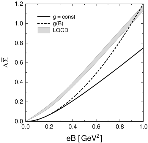
Figure 1: Normalized average $q\bar{q}$ condensate as a function of $eB$. Solid and dashed lines correspond to constant and $B$-dependent couplings. LQCD results from Ref. [92] (gray band) are added for comparison.

The effect of magnetic catalysis can be observed from Fig. 1, where we show the behavior of the normalized averaged light quark condensate as a function of the magnetic field, for $eB$ up to 1 GeV². Following Ref. [92], we use the definitions

$$\Delta\bar{\Sigma}(B)\ =\ \dfrac{\Delta\Sigma_{u}(B)+\Delta\Sigma_{d}(B)}{2}\ ,\qquad\qquad\Delta\Sigma_{f}(B)=-\frac{2\,m_{c}\,[\phi_{f}(B)-\phi_{f}^{0}]}{D^{4}}\ ,$$ (127)

where $D=(135\times 86)^{1/2}$ MeV is a phenomenological normalization constant. Solid and dashed lines correspond to constant and $B$-dependent couplings, respectively. Although the curves do not show an accurate fit to lattice data (gray band, taken from Ref. [92]), it is seen that the model is able to reproduce qualitatively the effect of magnetic catalysis. We have seen that a better agreement could be achieved using a parameter set that leads to lower values of the quark masses; however, this would hinder the analysis of the rho meson mass, since the latter would lie below the quark-antiquark production threshold even for $B=0$. Additionally, we have checked that the choice of a 3D-cutoff (within the MFIR scheme) leads in general to even lower values of $\Delta\bar{\Sigma}$, increasing the difference with LQCD results.

V.2 Neutral mesons

Let us analyze our results for the effect of the magnetic field on meson masses. We start with the neutral sector. As well known, for vanishing external field pseudoscalar mesons mix with “longitudinal” axial vector mesons. Now, as discussed in Sec. III.2, for nonzero $B$ the mixing also involves neutral vector mesons with spin projection $S_{z}=0$ (corresponding to the polarization state $c=2$). The four lowest mass states of this sector are to be identified with the physical states $\tilde{\pi}^{0}$, $\tilde{\eta}$, $\tilde{\rho}^{\,0}$ and $\tilde{\omega}$, where the particle names are chosen according to the spin-isospin composition of the states in the limit of vanishing external field, see Eq. (55).

Figure 2: Masses of neutral mesons with spin projection $S_{z}=0$ as functions of $eB$. Solid (dashed) lines correspond to constant ($B$-dependent) couplings.

The masses of these particles can be determined from Eq. (53). In Fig. 2 we show their behavior with the magnetic field, for constant and $B$-dependent couplings (solid and dashed lines, respectively). In the case of $\tilde{\rho}^{\,0}$ and $\tilde{\omega}$ mesons, for $B=0$ one has $m_{\rho}=m_{\omega}=775$ MeV, close to the quark-antiquark production threshold —which arises from the lack of confinement of the model— given by $2M_{d}(B=0)=800$ MeV. As can be seen from the figure, since $m_{\tilde{\rho}^{0}}$ and $m_{\tilde{\omega}}$ increase with the magnetic field, they overcome the threshold (shown by the dotted line) at relatively low values of $eB$. Beyond this limit, although one could obtain some results through analytic continuation [34, 72], pole masses would include an unphysical absorptive part, becoming relatively less reliable. For clarity, we display in Fig. 2 just the curves for $m_{\tilde{\rho}^{0}}$ and $m_{\tilde{\omega}}$ that correspond to the case of a constant value of the coupling $g$; in the case of the $B$-dependent coupling $g(B)$, the situation is entirely similar. It is also worth mentioning that the results for the $\tilde{\eta}$ and $\tilde{\omega}$ masses should be taken only as indicative, since a more realistic calculation would require a three-flavor version of the model in which flavor-mixing effects could be fully taken into account.

Regarding the neutral pion mass, in Fig. 3 we compare our results with those obtained in previous works [22, 72] and those corresponding to LQCD calculations, in which quenched Wilson fermions [52], dynamical staggered quarks [15, 52, 93] and improved staggered quarks [53] are considered. Although LQCD studies do not take into account flavor mixing (they deal with individual flavor states), according to the analysis in Ref. [72] the lightest meson mass is expected to be approximately independent of the value of the mixing parameter $\alpha$. It is also worth noticing that LQCD results have been obtained using different methods and values of the pion mass at $B=0$. In the figure we show the results obtained for NJL-like models in which different meson sectors have been taken into account. Left and right panels correspond to $g={\rm constant}$ and $g=g(B)$ [given by Eqs. (125-126)], respectively. If one considers just the pseudoscalar sector (red dotted lines), when $g$ is kept constant the behavior of $m_{\tilde{\pi}^{0}}$ with the magnetic field is found to be non monotonic, deviating just slightly from its value at $B=0$. In contrast, as seen from the right panel of Fig. 3, if one lets $g$ to depend on the magnetic field the mass shows a monotonic decrease, reaching a reduction of about 30% at $eB=1$ GeV². This suppression is shown to be in good agreement with LQCD results. When the mixing with the vector sector is considered, the results for both constant and $B$-dependent couplings (red dash-dotted lines in left and right panels) are similar to each other and monotonically decreasing, lying however quite below LQCD predictions. Finally, if the mixing with axial vector mesons is also included (solid lines) we obtain, for both constant and $B$-dependent couplings, a monotonic decrease which is in good qualitative agreement with LQCD calculations for the studied range of $eB$. One may infer that the incorporation of axial vector mesons, being the chiral partners of vector mesons, leads to cancellations that help to alleviate the magnitude of the neutral pion mass suppression. Their inclusion into the full picture leads to relatively more robust results, in good agreement with LQCD calculations, and is in fact one of the main takeaways of this work.

Figure 3: Normalized mass of the $\tilde{\pi}^{0}$ meson as a function of $eB$, for the case of constant (left panel) and $B$-dependent couplings (right panel). Red dotted and dash-dotted lines show the results from models that do not include the axial vector meson sector. The bands and the fat squares correspond to LQCD results quoted in Refs. [15, 52, 93, 53].

Let us discuss the composition of the $\tilde{\pi}^{0}$ state. The values of the coefficients associated with the spin-isospin decomposition given in Eq. (55) are quoted in the upper part of Table 1 for $eB=0$, 0.5 GeV² and 1 GeV². Those associated with the spin-flavor decomposition, defined in the same way as in Eq. (56), are given in the lower part of the table. We quote the values corresponding to the model in which the couplings constants do not depend on the magnetic field; the results are qualitatively similar for the case of $B$-dependent couplings. One finds that while the mass eigenvalues do not depend on whether $B$ is positive or negative, the corresponding eingenvectors do; the relative signs in Table 1 correspond to the choice $B>0$. We consider first the results for vanishing magnetic field. It is seen that, due to the wellknown $\pi$-a₁ mixing, the $\tilde{\pi}^{0}$ state has already some axial vector component. We also note that even though $\alpha$ is relatively small (in our parametrization we have taken $\alpha=0.114$, to be compared with its maximum possible value 1/2), the effect of flavor mixing is already very strong; the spin-isospin composition is clearly dominated by the $\pi_{3}$ component, which is given by an antisymmetric equal-weight combination of $u$ and $d$ quark flavors. This can be understood by noticing that, as soon as $\alpha$ is different from zero, the U(1)_A symmetry gets broken. The state $\pi_{3}$ is then the only one that remains being a pseudo-Goldstone boson, which forces the lowest-mass state $\tilde{\pi}^{0}$ to be dominated by the $\pi_{3}$ component. In the presence of the magnetic field, the mixing is expected to be modified, since the external field distinguishes between flavor components $\pi_{u}$ and $\pi_{d}$ instead of isospin states. From the upper part of Table 1 it is seen that, even for the relatively small value of $\alpha$ considered here, the mass state $\tilde{\pi}^{0}$ is dominated by the $\pi_{3}$ component ($|c^{\tilde{\pi}^{0}}_{\pi_{3}}|^{2}\gtrsim 0.97$) for the full range of values of $eB$ up to 1 GeV². This means that the dominance of the flavor composition over the isospin composition will occur only for extremely large values of $eB$. In any case, from the values in Table 1 one can still observe some effect of the magnetic field on the composition of the $\tilde{\pi}^{0}$ state: when $eB$ increases, it is found that there is a slight decrease of the $\pi_{3}$ component in favor of the others. In addition, a larger weight is gained by the $u$-flavor components, as one can see by looking at the entries corresponding to the spin-flavor states (lower part of Table 1): one has $|c^{\tilde{\pi}^{0}}_{\pi_{u}}|^{2}+|c^{\tilde{\pi}^{0}}_{\rho_{u,2}}|^{2}+|c^{\tilde{\pi}^{0}}_{a_{u,L}}|^{2}=0.50(0.64)$ for $eB=0(1.0)$ GeV². This can be understood by noticing that the magnetic field is known to reduce the mass of the lowest neutral meson state [50, 52, 53]; for large $eB$ one expects the lowest mass state ($\tilde{\pi}^{0}$) to have a larger component of the quark flavor that couples more strongly to the magnetic field (i.e., the $u$ quark). Concerning the vector meson components of the $\tilde{\pi}^{0}$ state, it is seen that they are completely negligible at low values of $eB$, reaching a contribution similar to the one of the axial vector meson ($\simeq 0.5\ \%$) at $eB=1$ GeV².

$eB\ [{\rm GeV}^{2}]$		Spin-isospin composition
		$c^{\tilde{\pi}^{0}}_{\pi_{3}}$	$c^{\tilde{\pi}^{0}}_{\pi_{0}}$	$c^{\tilde{\pi}^{0}}_{\rho_{3,2}}$	$c^{\tilde{\pi}^{0}}_{\rho_{0,2}}$	$c^{\tilde{\pi}^{0}}_{a_{3,L}}$	$c^{\tilde{\pi}^{0}}_{a_{0,L}}$
0		0.998	0	0	0	-0.067	0
0.5		0.993	0.084	0.016	0.060	-0.063	-0.011
1.0		0.987	0.141	0.010	0.057	-0.058	-0.012
$eB\ [{\rm GeV}^{2}]$		Spin-flavor composition
		$c^{\tilde{\pi}^{0}}_{\pi_{u}}$	$c^{\tilde{\pi}^{0}}_{\pi_{d}}$	$c^{\tilde{\pi}^{0}}_{\rho_{u,2}}$	$c^{\tilde{\pi}^{0}}_{\rho_{d,2}}$	$c^{\tilde{\pi}^{0}}_{a_{u,L}}$	$c^{\tilde{\pi}^{0}}_{a_{d,L}}$
0		0.706	-0.706	0	0	-0.047	0.047
0.5		0.707	-0.704	0.011	0.006	-0.047	0.047
1.0		0.798	-0.598	0.048	0.033	-0.050	0.032

Table 1: Composition of the $\tilde{\pi}^{0}$ meson mass eigenstate for selected values of $eB$. Relative signs hold for the choice $B>0$. The upper table corresponds to the spin-isospin decomposition, as given in Eq. (55), while the lower one corresponds to a spin-flavor decomposition.

In addition, as discussed in Sec. III.2, the neutral sector includes states with spin projections $S_{z}=\pm 1$, i.e., spin parallel to the direction of the magnetic field. We consider here the effect of the magnetic field on vector meson states, whose masses can be obtained from the submatrices $\hat{\mathbf{G}}^{(\pm 1,+)}$ in Eq. (50). Since in this sector vector meson and axial vector meson states do not mix, the analysis is entirely equivalent to the one carried out in Ref. [72], where the axial vector sector was not taken into account. As stated in Sec. III.3, it is easy to see that the mass matrices involving the states $\rho_{0,c}$ and $\rho_{3,c}$, with $c=1,3$ are diagonalized by rotating from the isospin basis to a flavor basis $(\rho_{u,c},\rho_{d,c})$ given by Eq. (56); moreover, the masses of these mesons turn out to be equal for polarization states $c=1$ ($S_{z}=+1$) and $c=3$ ($S_{z}=-1$).

The numerical results for $\rho_{u}$ and $\rho_{d}$ meson masses as functions of the magnetic field are shown in Fig. 4. It is seen that both masses increase with $B$, the enhancement being larger in the case of the $\rho_{u}$ mass; this can be understood from the larger (absolute) value of the $u$-quark charge, which measures the coupling with the magnetic field. The results are similar for the case of constant and $B$-dependent couplings, corresponding to solid and dashed lines in the figure, respectively. The dotted lines indicate the mass thresholds for $q\bar{q}$ pair production, given by $m_{\rho_{f}}^{({\rm th})}=M_{d}+\sqrt{M_{d}^{2}+2B_{d}}$. As discussed in Ref. [72], this threshold is given by a situation in which the spins of both the quark and antiquark components of the $\rho_{f}$ meson are aligned (or anti-aligned) with the magnetic field; thus, one of the fermions lies in its lowest Landau level, while the other one lies in its first excited Landau level. In comparison with the $S_{z}=0$ threshold $2M_{d}$, for $S_{z}=\pm 1$ the threshold $m_{\rho_{f}}^{({\rm th})}$ grows faster with $B$. For a constant coupling $g$, this allows the values of $m_{\rho_{u}}$ and $m_{\rho_{d}}$ to remain below the threshold for the studied range of magnetic fields. On the other hand, in the case of a $B$-dependent coupling $g(B)$ the $\rho_{u}$ meson is found to become unstable for $eB$ somewhat larger than $0.6$ GeV². Our results for the $\rho_{u}$ mass are found to be in agreement, within errors, with values obtained through LQCD calculations, also shown in Fig. 4 [52].

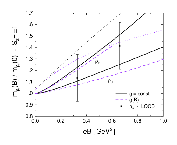
Figure 4: Masses of $\rho$ mesons with spin projection $S_{z}=\pm 1$ as functions of $eB$. Solid and dashed lines correspond to constant and $B$-dependent couplings; dotted lines indicate $q\bar{q}$ production thresholds. LQCD data for $\rho_{u}$ from Ref. [52] are included for comparison.

V.3 Charged mesons

As discussed in Sec. IV, to study the lowest lying charged meson states in the presence of the magnetic field one has to consider the Landau modes $\ell=-1$ and $\ell=0$. For $\ell=-1$, the lowest mass state is the one that we have denoted as $\rho_{1}$, which does not get mixed with any other state. The corresponding pole mass $m_{\rho^{+}}$ can be obtained from Eq. (116), while the lowest energy for this state is given by $E_{\rho^{+}}=\sqrt{m_{\rho^{+}}^{2}-B_{e}}$, see Eq. (119).

In Fig. 5 we show our numerical results for $E_{\rho^{+}}$ as a function of $eB$, normalized by the value of the $\rho$ mass at $B=0$. Black solid and dashed lines correspond to the cases of constant and $B$-dependent couplings, respectively, where $g(B)$ is given by Eqs. (125-126). It can be seen that for $g=\mbox{constant}$ the results differ considerably from those obtained in a similar model [73] which instead does not take into account the presence of axial vector mesons (red dotted line in the figure). On the contrary, for $g=g(B)$ (red dash-dotted line) they remain basically unchanged. In fact, here the differences between models that include or not axial vector mesons do not arise from direct mixing effects (the $\rho_{1}$ state does not mix with axial vectors) but from the fact that axial vector states mix with pions already for $B=0$; this leads to some change in the model parameters so as to get consistency with the phenomenological inputs. In any case, it is found that —as in the case of neutral mesons— the results from the full model (black solid and dashed lines) appear to be rather robust: they show a similar behavior either for constant or $B$-dependent couplings, and this behavior is shown to be in good agreement with LQCD calculations [60, 46, 52], also shown in the figure. Notice that our results, as those from LQCD, are not consistent with $\rho^{+}$ condensation for the considered range of values of $eB$. The curve corresponding to the lowest energy state of a pointlike $\rho^{+}$ meson as a function of $eB$ is shown for comparison.

It is worth mentioning that our results are qualitatively different from those obtained in other works in the framework of two-flavor NJL-like models [19, 31], which do find $\rho^{+}$ meson condensation for $eB\sim 0.2$ to $0.6$ GeV². As discussed in Refs. [73, 81], in those works Schwinger phases are neglected and it is assumed that charged $\pi$ and $\rho$ mesons lie in zero three-momentum states (i.e., meson wavefunctions are approximated by plane waves). Here we use, instead, an expansion of meson fields in terms of the solutions of the corresponding equations of motion for nonzero $B$, taking properly into account the presence of Schwinger phases in quark propagators. In fact, as shown in Ref. [81], the plane wave approximation may have a dramatic incidence on these numerical results, implying a substantial change in the behavior of the $\rho^{+}$ mass for the $\ell=-1$ Landau mode.

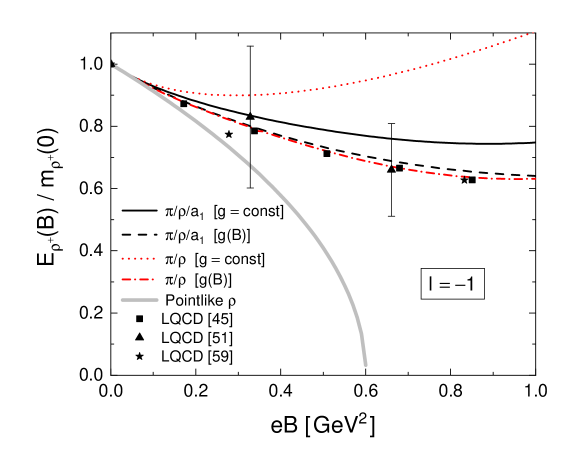
Figure 5: Energy of the $\rho^{+}$ meson as a function of $eB$ for the lowest Landau mode $\ell=-1$ and vanishing component of the momentum in the direction of $\vec{B}$. Values are normalized to the $\rho^{+}$ mass at zero external field. Black solid and dashed lines correspond to constant and $B$-dependent couplings, respectively. Red dotted and dash-dotted lines show results from models that do not include axial vector mesons, while the light gray line corresponds to a pointlike $\rho^{+}$. For comparison, lattice QCD data quoted in Refs. [60, 46, 52] are also included.

In the case of the mode $\ell=0$, as discussed in Sec. IV, the lowest mass state $\pi^{+}$ is given in general by a mixing between the states that we have denoted as $\pi$, $\rho_{2}$, $a_{L}$ and $a_{1}$. The corresponding pole mass $m_{\pi^{+}}$ can be obtained from Eq. (120), while the lowest energy for this state is given by $E_{\pi^{+}}=\sqrt{m_{\pi^{+}}^{2}+B_{e}}$, see Eq. (123). Our numerical results are presented in Fig. 6, where, for the sake of comparison with LQCD values, we plot the values of the difference $E_{\pi^{+}}(B)^{2}-E_{\pi^{+}}(0)^{2}$ as a function of $eB$. Once again, black solid and dashed lines correspond to the cases of constant and $B$-dependent couplings, respectively. We also include for comparison the results obtained from similar NJL-like models that just include the pseudoscalar meson sector (red dotted line), or just include the mixing between the pseudoscalar and vector meson sectors (red dash-dotted line), neglecting the effect of the presence of axial vector mesons. It can be seen that the inclusion of the axial vector meson sector leads to an improvement of the agreement with LQCD data quoted in Refs. [15, 46, 53], also shown in the figure.

It is interesting to point out that, for large external magnetic fields, the values from LQCD shown in Fig. 6 lie well below the curve that corresponds to a pointlike pion. From Eq. (123), it is easy to see that to reproduce these results one should get a negative value of the pole mass squared, $m_{\pi^{+}}^{2}<0$. In fact, this is what we obtain from our NJL-like model if we assume that the coupling constants do not depend on $B$ (solid line in the figure). The appearance of an imaginary pole mass does not signal the existence of a meson condensation, since meson energies are still positive quantities; indeed, the presence of the magnetic field generates a zero-point motion in the plane perpendicular to $\vec{B}$ that induces an “effective magnetic mass” $\sqrt{m_{\pi^{+}}^{2}+B_{e}}$. Notice that in this case some analytical expressions have to be revised. The corresponding changes, basically related with the normalization of polarization vectors, are indicated in App. E. In contrast, for $B$-dependent couplings one does not observe a large variation of the $\pi^{+}$ pole mass for the studied range of $eB$; the energy is essentially dominated by the magnetic field. Thus, the curve shown in Fig. 6 (black dashed line) turns out to be approximately coincident with the one corresponding to a pointlike charged pion. We remark that our numerical results indicate a monotonic enhancement of the charged pion energy with the magnetic field, in contrast with the nonmonotic behavior found in some recent LQCD simulations (green circles in the figure) [53]. It would be interesting to get more insight on this open issue from other effective models and further LQCD calculations.

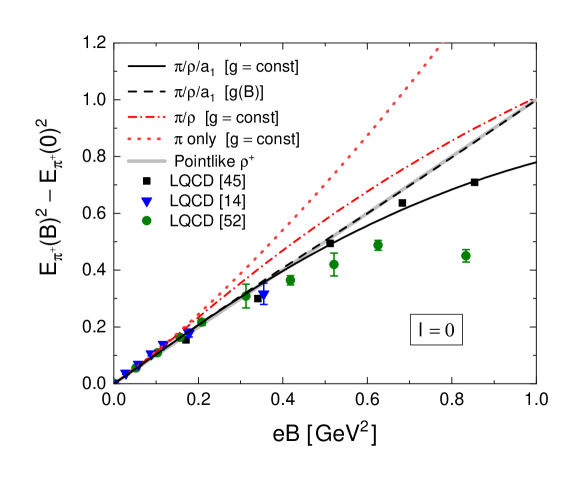
Figure 6: Squared energy of the $\pi^{+}$ mass eigenstate for the Landau mode $\ell=0$ and vanishing component of the momentum in the direction of $\vec{B}$. Values are given with respect to the squared $\pi^{+}$ mass for vanishing external field. Black solid and dashed lines correspond to constant and $B$-dependent couplings, respectively. Red dotted and dash-dotted lines show results from models that do not include axial vector mesons, while the light gray line corresponds to a pointlike $\pi^{+}$. For comparison, lattice QCD data quoted in Refs. [15, 46, 53] are also included.

To conclude this section, let us discuss the state composition of the charged pion mass state. In Table 2 we quote our results for the coefficients of the linear combination in Eq. (124) for some values of $eB$, considering both the cases $g=\mbox{constant}$ and $g(B)$ (upper and lower parts of the table, respectively). We also include the values of the normalized squared $\pi^{+}$ pole masses. For $B=0$, as well known, in these type of model the pion mass eigenstate is obtained from a mixing between the pseudoscalar state $\pi$ and the longitudinal part of the axial-vector state ($a_{L}$, in our notation). Then, for nonzero $B$, the mixing between the states $\rho_{2}$ and $a_{1}$ is also turned on. As stated, for $g=\mbox{constant}$ the value of $m_{\pi^{+}}^{2}$ becomes negative if the magnetic field is increased; this occurs at $eB\simeq 0.5$ GeV². As shown in the upper part of Table 2, when approaching this point the mass eigenstate turns out to be strongly dominated by the axial vector states $a_{1}$ and $a_{L}$, which have similar weights. For larger values of $eB$ the absolute value of $m_{\pi^{+}}^{2}$ gets increased, and once again the $\pi^{+}$ state becomes dominated by the pseudoscalar $\pi$ contribution. Notice, however, that for $eB=1$ GeV the contributions of other states are nonnegligible; moreover, it is seen that the coefficients $c^{\pi^{+}}_{a_{1}}$ and $c^{\pi^{+}}_{a_{L}}$ become imaginary. On the contrary, as shown in the lower part of the table, for $g=g(B)$ these effects are not observed in the studied range of values of the external field. As mentioned above, in this case the $\pi^{+}$ pole mass does not show qualitative changes with $eB$; the main effect of the magnetic field is the enhancement of axial vector components, each of them reaching about $1/4$ of the state composition at $eB=1$ GeV², while the remaining 1/2 fraction is almost saturated by the $\pi$ component. As stated, recent LQCD data support a negative value of $m_{\pi^{+}}^{2}$ for large magnetic fields. It would be also interesting to get information from lattice calculations on the state composition, in particular, in the region $eB\sim 1$ GeV².

$eB$ [GeV2]	$m_{\pi^{+}}(B)^{2}/m_{\pi^{+}}(0)^{2}$	State composition ($g=\mbox{constant}$)
			$c^{\pi^{+}}_{\pi}\$	$c^{\pi^{+}}_{\rho_{2}}\$	$c^{\pi^{+}}_{a_{1}}\$	$c^{\pi^{+}}_{a_{L}}\$
0	1		0.998	0	0	$-0.067$
0.5	0.006		0.174	$-0.025$	0.697	0.697
1.0	-10.29		0.879	$-0.210$	$-0.201\,i$	$-0.378\,i$
$eB$ [GeV2]	$m_{\pi^{+}}(B)^{2}/m_{\pi^{+}}(0)^{2}$	State composition ($g=g(B)$)
			$c^{\pi^{+}}_{\pi}\$	$c^{\pi^{+}}_{\rho_{2}}\$	$c^{\pi^{+}}_{a_{1}}\$	$c^{\pi^{+}}_{a_{L}}\$
0	1		0.998	0	0	$-0.067$
0.5	1.18		0.924	$-0.137$	0.287	0.214
1.0	0.95		0.651	$-0.168$	0.545	0.501

Table 2: Normalized squared pole mass and composition of the $\pi^{+}$ meson mass eigenstate for selected values of $eB$.

VI Summary & Conclusions

In this work we have studied the mass spectrum of light pseudoscalar and vector mesons in the presence of an external uniform and static magnetic field $\vec{B}$, introducing the effects of the mixing with the axial vector meson sector. The study has been performed in the framework of a two-flavor NJL-like model that includes isoscalar and isovector couplings in the scalar-pseudoscalar and vector-axial vector sector, as well as a flavor mixing term in the scalar-pseudoscalar sector. For simplicity, the coupling constants of the vector and axial vector sector have been taken to be equal. The ultraviolet divergences associated to the nonrenormalizability of the model have been regularized using the magnetic field independent regularization method, which has been shown to be free from unphysical oscillations and to reduce the dependence of the results on the model parameters [83]. Additionally, we have explored the possibility of using magnetic field dependent coupling constants $g(B)$ to account for the effect of the magnetic field on sea quarks.

As well known, for vanishing external field pseudoscalar mesons mix with “longitudinal” axial vector mesons. Now, the presence of an external uniform magnetic field breaks isospin (due to the different quark electric charges) and full rotational symmetry, allowing for a more complex meson mixing pattern than in vacuum. The mixing structure is constrained by the remaining unbroken symmetries, in such a way that the mass matrices —written in a basis of polarization states— can be separated into several “boxes”.

In the case of neutral mesons, Schwinger phases cancel and the polarization functions become diagonal in the usual momentum basis. Since mesons can be taken at rest, rotational invariance around $\hat{B}$ implies that $S_{z}$ (the spin in the field direction) is a good quantum number to characterize these states. The aforementioned symmetries restrict the allowed mixing in the original $20\times 20$ mass matrix, which can be decomposed as a direct sum of subspaces of states with $s_{z}=-1$, 0, and 1. For $s_{z}=\pm 1$ (spin parallel to $\vec{B}$), it is seen that vector mesons do not mix with other sectors, and the mass eigenstates are those of the flavor basis ($\rho_{u},\rho_{d}$). We have shown that the corresponding masses increase with $B$ in qualitative agreement with LQCD, within uncertainties. For $s_{z}=0$ (spin perpendicular to $\vec{B}$), scalar mesons turn out to get decoupled from other states and therefore have been disregarded in our analysis. Meanwhile, pseudoscalar mesons mix with vector and axial vector mesons whose polarization states are parallel to $\vec{B}$. The four lowest mass states of this sector are to be identified with the physical states $\tilde{\pi}^{0}$, $\tilde{\eta}$, $\tilde{\rho}^{\,0}$ and $\tilde{\omega}$. Regarding $m_{\tilde{\rho}^{0}}$ and $m_{\tilde{\omega}}$, we have found that they get increased with the magnetic field, in such a way that they overcome a $q\bar{q}$ decay threshold —which arises from the lack of confinement of the model— at relatively low values of $eB$. Concerning $m_{\tilde{\eta}}$, a slight decrease with $B$ is observed.

The impact of the inclusion of the axial vector meson sector on the mass of the lightest state $\tilde{\pi}^{0}$, identified with the neutral pion, is actually one of the main focus of our work. We have found that when axial vector mesons are taken into account, $m_{\tilde{\pi}^{0}}$ displays a monotonic decreasing behavior with $B$ in the studied range $eB<1$ GeV², which is in good qualitative agreement with LQCD calculations for both $g={\rm constant}$ and $g(B)$. Thus, our current results represent an improvement over previous analyses that take into account just the mixing with the vector meson sector, or no mixing at all. When no mixing is considered, the behavior of $m_{\tilde{\pi}^{0}}$ with $B$ is non monotonic when $g$ is kept constant, deviating just slightly from its value at $B=0$. Only when $g$ is allow to depend on the magnetic field one obtains a decreasing behavior which resembles LQCD results. Even though the inclusion of the vector sector leads to a reduction in $m_{\tilde{\pi}^{0}}$ together with a consistent decreasing trend, the values lie quite below LQCD predictions, for both $g$ and $g(B)$. We therefore conclude that the inclusion of axial mesons is important since it leads to more robust results for the neutral pion mass, even independently of the assumption of a magnetic field dependent coupling constant. Regarding the composition of the $\tilde{\pi}^{0}$ state, we have found that it is largely dominated by the isovector component $\pi_{3}$ ($|c^{\tilde{\pi}^{0}}_{\pi_{3}}|^{2}\gtrsim 0.97$) for the studied range of values of $eB$. In terms of flavor composition, a larger weight is gained by $u$-flavor components for large values of $B$, which can be understood from the fact that the $u$ quark couples more strongly to the magnetic field.

In the case of charged mesons, the corresponding polarization functions are diagonalized by expanding meson fields in appropriate Ritus-like bases, so as to account for the effect of nonvanishing Schwinger phases. Once again, the symmetries of the system constrain the allowed mixing matrices, which also depend on the value of the meson Landau level $\ell$. For $\ell=-1$ one has only one vector and one axial vector polarization states. Moreover, they do not mix with any other particle state. Thus, for $\ell=-1$ the effect of the inclusion of axial vector mesons on the $\rho^{+}$ mass comes solely from the model parametrization, which is affected by the presence of $\pi$-a₁ mixing at $B=0$. Our results show that when the axial vector sector is included, the energy $E_{\rho^{+}}=\sqrt{m_{\rho^{+}}^{2}-B_{e}}$ of this state undergoes a considerable reduction, leading to a decreasing behavior which is in qualitative agreement with LQCD predictions, independently of the assumption of a $B$-dependent coupling constant. However —in accordance to LQCD calculations and with our previous results within NJL-like models that do not include axial vectors [73, 81]— we find that $E_{\rho^{+}}$ does not vanish for any considered value of the magnetic field, a fact that can be relevant in connection with the occurrence of $\rho^{+}$ meson condensation for strong magnetic fields.

For $\ell=0$ only three polarization vectors are linearly independent, and the pion mixing subspace is given by $\pi^{+}\mhyphen\rho^{+}\mhyphen{\rm a}_{1}^{+}$ for only certain polarizations states. The lowest mass state in this sector can be identified with the $\pi^{+}$, whose lowest energy is given by $E_{\pi^{+}}=\sqrt{m_{\pi^{+}}^{2}+B_{e}}$. Our results show that, even though vector mixing already induces a softening in the enhancement of the pion energy with $B$, the inclusion of the axial vector meson sector reinforces this softening, leading to an improved agreement with LQCD predictions. Remarkably, for a constant coupling $g$ and magnetic fields stronger than $eB=0.4$ GeV², we obtain values of the pion energy which lie well below the ones correspoding to a pointlike pion, in concordance with LQCD results in Refs. [46, 53]. On the other hand, in the case of a $B$-dependent coupling we find that the pole mass becomes approximately constant; as a result, the energy is basically coincident with the one corresponding to a pointlike charged pion. As for the $\pi^{+}$ state composition, we have seen that in general the magnetic field induces a mixing between all states by increasing the contribution from vector and axial vector components.

In view of the above results, one can conclude that the inclusion of axial vector mesons leads to more robust results and improves the agreement between NJL-like models and LQCD calculations. Still, issues about meson masses and mass eigenstate compositions at large magnetic fields are still open, and further results from LQCD and effective models of strong interactions would be welcome.

Appendices

A Conventions and notation

Throughout this section we use the Minkowski metric $\eta^{\mu\nu}=\mbox{diag}(1,-1,-1,-1)$, while for a space-time coordinate four-vector $x^{\mu}$ we adopt the notation $x^{\mu}=(t,\vec{x})$, with $\vec{x}=(x^{1},x^{2},x^{3})$.

We study interactions between charged particles and an external electromagnetic field ${\cal A}^{\mu}(x)$. The electromagnetic field strength $F^{\mu\nu}$ and its dual ${{\tilde{F}}^{\mu\nu}}$ are given by

$$F^{\mu\nu}=\partial^{\mu}\mathcal{A}^{\nu}-\partial^{\nu}\mathcal{A}^{\mu}\ ,\qquad\qquad{{\tilde{F}}^{\mu\nu}}=\frac{1}{2}\,\epsilon^{\mu\nu\alpha\beta}F_{\alpha\beta}\ ,$$ (A.1)

where the convention $\epsilon^{0123}=+1$ is used. We consider in particular the situation in which one has a static and uniform magnetic field $\vec{B}$; without losing generality, we choose the axis 3 to be parallel to $\vec{B}$, i.e., we take $\vec{B}=(0,0,B)$ (note that $B$ can be either positive or negative). Moreover, defining

$$\hat{F}^{\mu\nu}=\frac{1}{B}\,F^{\mu\nu}\ ,\qquad\qquad{\hat{\tilde{F}}^{\mu\nu}}=\frac{1}{B}\,{\tilde{F}}^{\mu\nu}$$ (A.2)

for $i,j=1,2,3$ one has

$$\hat{F}^{0\nu}=0\ , \qquad\hat{F}^{ij}=-\epsilon_{ij3}\ ,$$

$${\hat{\tilde{F}}^{ij}}=0\ , \qquad{\hat{\tilde{F}}^{0k}}=-\,\epsilon^{0kij}\epsilon_{ij3}/2\ ,$$ (A.3)

i.e. the relevant components of the tensors are $\hat{F}^{12}=-\hat{F}^{21}=-1$, ${\hat{\tilde{F}}^{03}}=-{\hat{\tilde{F}}^{30}}=-1$.

Since isotropy is broken by the particular direction of the external field $\vec{B}$, it is convenient to separate the metric tensor into “parallel” and “perpendicular” pieces,

$$\eta_{\parallel}^{\mu\nu}=\mbox{diag}(1,0,0,-1)\ ,\qquad\qquad\eta_{\perp}^{\mu\nu}=\mbox{diag}(0,-1,-1,0)\ .$$ (A.4)

In addition, given a four-vector $v^{\mu}$, it is useful to define “parallel” and “perpendicular” vectors

$$v_{\parallel}^{\mu}=(v^{0},0,0,v^{3})\ ,\qquad\qquad v_{\perp}^{\mu}=(0,v^{1},v^{2},0)\ .$$ (A.5)

B Neutral meson polarization functions

According to Eq. (27), the polarization functions for neutral mesons can be written as a sum of flavor-dependent functions $\Sigma_{MM^{\prime}}^{f}(q)$. The latter, in turn, can be written in terms of a set of Lorentz covariant tensors as

$$\Sigma_{MM^{\prime}}^{f}(q)=\sum_{i=1,n_{mm^{\prime}}}c_{mm^{\prime},i}^{f}(q_{\perp}^{2},q_{\parallel}^{2})\ \mathbb{O}_{MM^{\prime}}^{(i)}(q)\ .$$ (B.1)

Here, $M=\pi_{b},\rho_{b}^{\mu},a_{b}^{\mu}$ correspond to $m=\pi,\rho,a$, and the same is understood for $M^{\prime}$ and $m^{\prime}$. The coefficients $c_{mm^{\prime},i}^{f}$ are scalar functions, while the tensors $\mathbb{O}_{MM^{\prime}}^{(i)}$ carry the corresponding Lorentz structures. Notice that the number of terms in the sum, $n_{mm^{\prime}}$, depends on the combination $mm^{\prime}$ considered. The scalar coefficients can be expressed as

$$c_{mm^{\prime},i}^{f}(q_{\perp}^{2},q_{\parallel}^{2})\ =\ \frac{N_{c}}{8\pi^{2}}\int_{0}^{\infty}dz\,\int_{-1}^{1}dv\ e^{-z\,\phi_{0}^{f}(q_{\perp},q_{\parallel},v,z)}\;\gamma_{mm^{\prime},i}^{f}(q_{\perp}^{2},q_{\parallel}^{2},v,z)\ ,$$ (B.2)

where

$$\phi_{0}^{f}(q_{\perp},q_{\parallel},v,z)\ =\ M_{f}^{2}-\frac{1-v^{2}}{4}\;q_{\parallel}^{2}+\frac{\cosh(z\,B_{f})-\cosh(v\,z\,B_{f})}{2\,z\,B_{f}\,\sinh(z\,B_{f})}\;\vec{q}_{\perp}^{\;2}\ ,$$ (B.3)

with $B_{f}=|BQ_{f}|$. In the following we list the sums associated to each polarization function, together with the explicit expressions of the functions $\gamma_{mm^{\prime},i}^{f}(q_{\perp}^{2},q_{\parallel}^{2},v,z)$ corresponding to the coefficients $c_{mm^{\prime},i}^{f}(q_{\perp}^{2},q_{\parallel}^{2})$. For brevity, the arguments of $c_{mm^{\prime},i}^{f}$ and $\gamma_{mm^{\prime},i}^{f}$ are not explicitly written.

The $\pi\pi$ polarization function is a scalar, therefore there is only one coefficient $c_{\pi\pi,1}^{f}$, and $\mathbb{O}_{\pi_{b}\pi_{b^{\prime}}}^{(1)}(q)=1$. One has

$$\Sigma_{\pi_{b}\pi_{b^{\prime}}}^{f}(q)\ =\ c_{\pi\pi,1}^{f}\ ,$$ (B.4)

while the associated function $\gamma_{\pi\pi,1}^{f}$ is given by

$$\gamma_{\pi\pi,1}^{f} = \left(M_{f}^{2}+\frac{1}{z}+\frac{1-v^{2}}{4}\;q_{\parallel}^{2}\right)\,\frac{B_{f}}{\tanh(z\,B_{f})}$$ (B.5)

$$+\,\frac{B_{f}^{2}}{\sinh^{2}(z\,B_{f})}\left[1-\frac{\cosh(z\,B_{f})-\cosh(v\,z\,B_{f})}{2B_{f}\sinh(z\,B_{f})}\;{\vec{q}}_{\perp}^{\;2}\right]\ .$$

Analogously, for the $\sigma\sigma$ polarization function we have

$$\Sigma_{\sigma_{b}\sigma_{b^{\prime}}}^{f}(q)\ =\ c_{\sigma\sigma,1}^{f}\ ,$$ (B.6)

while

$$\gamma_{\sigma\sigma,1}^{f} = \left(-M_{f}^{2}+\frac{1}{z}+\frac{1-v^{2}}{4}\;q_{\parallel}^{2}\right)\,\frac{B_{f}}{\tanh(z\,B_{f})}$$ (B.7)

$$+\,\frac{B_{f}^{2}}{\sinh^{2}(z\,B_{f})}\left[1-\frac{\cosh(z\,B_{f})-\cosh(v\,z\,B_{f})}{2B_{f}\sinh[z\,B_{f}]}\;{\vec{q}}_{\perp}^{\;2}\right]\ .$$

For the $\rho\rho$ polarization the sum in Eq. (B.1) includes five terms. We find

$$\Sigma_{\rho_{b}^{\mu}\rho_{b^{\prime}}^{\nu}}^{f\;\mu\nu}(q)\ =\ c_{\rho\rho,1}^{f}\,\eta_{\parallel}^{\mu\nu}+c_{\rho\rho,2}^{f}\,\eta_{\perp}^{\mu\nu}+c_{\rho\rho,3}^{f}\,q_{\parallel}^{\mu}\,q_{\parallel}^{\nu}+c_{\rho\rho,4}^{f}\,q_{\perp}^{\mu}\,q_{\perp}^{\nu}+c_{\rho\rho,5}^{f}\,\big{(}q_{\perp}^{\mu}\,q_{\parallel}^{\nu}+q_{\parallel}^{\mu}\,q_{\perp}^{\nu}\big{)}\ ,$$ (B.8)

while the functions $\gamma_{\rho\rho,i}^{f}$ read

$$\gamma_{\rho\rho,1}^{f} = -\left(M_{f}^{2}+\frac{1-v^{2}}{4}\;q_{\parallel}^{2}\right)\frac{B_{f}}{\tanh(z\,B_{f})}-\frac{B_{f}^{2}}{\sinh^{2}(z\,B_{f})}$$

$$+\,\frac{B_{f}\big{[}\cosh(z\,B_{f})-\cosh(v\,z\,B_{f})\big{]}}{2\,\sinh^{3}[z\,B_{f}]}\;{\vec{q}}_{\perp}^{\;2}\ ,$$

$$\gamma_{\rho\rho,2}^{f} = -\left(M_{f}^{2}+\frac{1}{z}+\frac{1-v^{2}}{4}\;q_{\parallel}^{2}\right)\frac{B_{f}\cosh(v\,z\,B_{f})}{\sinh(z\,B_{f})}$$

$$+\,\frac{B_{f}\big{[}\cosh(z\,B_{f})-\cosh(v\,z\,B_{f})\big{]}}{2\,\sinh^{3}[z\,B_{f}]}\;{\vec{q}}_{\perp}^{\;2}\ ,$$

$$\gamma_{\rho\rho,3}^{f} = (1-v^{2})\,\frac{B_{f}}{2\,\tanh[z\,B_{f}]}\ ,$$

$$\gamma_{\rho\rho,4}^{f} = B_{f}\,\frac{\cosh(z\,B_{f})-\cosh(v\,z\,B_{f})}{\sinh^{3}(z\,B_{f})}\ ,$$

$$\gamma_{\rho\rho,5}^{f} = B_{f}\,\frac{\cosh(v\,z\,B_{f})-v\coth(z\,B_{f})\sinh(v\,z\,B_{f})}{2\,\sinh(z\,B_{f})}\ .$$ (B.9)

For the $aa$ polarization function we get

$$\Sigma_{a_{b}^{\mu}a_{b^{\prime}}^{\nu}}^{f\;\mu\nu}(q)\ =\ c_{aa,1}^{f}\,\eta_{\parallel}^{\mu\nu}+c_{aa,2}^{f}\,\eta_{\perp}^{\mu\nu}+c_{aa,3}^{f}\,q_{\parallel}^{\mu}\,q_{\parallel}^{\nu}+c_{aa,4}^{f}\,q_{\perp}^{\mu}\,q_{\perp}^{\nu}+c_{aa,5}^{f}\,\left(q_{\perp}^{\mu}\,q_{\parallel}^{\nu}+q_{\parallel}^{\mu}\,q_{\perp}^{\nu}\right)\ ,$$ (B.10)

while the functions $\gamma_{aa,i}^{f}$ are given by

$$\gamma_{aa,1}^{f} = -\left(-M_{f}^{2}+\frac{1-v^{2}}{4}\;q_{\parallel}^{2}\right)\frac{B_{f}}{\tanh(z\,B_{f})}-\frac{B_{f}^{2}}{\sinh^{2}(z\,B_{f})}$$

$$+\,\frac{B_{f}\big{[}\cosh(z\,B_{f})-\cosh(v\,z\,B_{f})\big{]}}{2\,\sinh^{3}[z\,B_{f}]}\;{\vec{q}}_{\perp}^{\;2}\ ,$$

$$\gamma_{aa,2}^{f} = -\left(-M_{f}^{2}+\frac{1}{z}+\frac{1-v^{2}}{4}\;q_{\parallel}^{2}\right)\frac{B_{f}\cosh(v\,z\,B_{f})}{\sinh(z\,B_{f})}$$

$$+\,\frac{B_{f}\big{[}\cosh(z\,B_{f})-\cosh(v\,z\,B_{f})\big{]}}{2\,\sinh^{3}[z\,B_{f}]}\;{\vec{q}}_{\perp}^{\;2}\ ,$$

$$\gamma_{aa,i}^{f} = \gamma_{\rho\rho,i}^{f}\quad\mbox{for}\quad i=3,4,5\ .$$ (B.11)

For the $\pi\rho$ and $\rho\pi$ polarization functions we get

$$\Sigma_{\pi_{b}\rho_{b^{\prime}}^{\mu}}^{f\;\mu}(q)\ =\ \Sigma_{\rho_{b}^{\mu}\pi_{b^{\prime}}}^{f\;\mu}(q)^{\,\ast}\ =\ c_{\pi\rho,1}^{f}\;\hat{\tilde{F}}^{\mu\alpha}\,q_{\parallel\alpha}$$ (B.12)

and

$$\gamma_{\pi\rho,1}^{f}\ =\ -is_{f}\,B_{f}M_{f}\ ,$$ (B.13)

with $s_{f}={\rm sign}(BQ_{f})$.

For the $\pi a$ and $a\pi$ polarization functions we get

$$\Sigma_{\pi_{b}a_{b^{\prime}}^{\mu}}^{f\;\mu}(q)\ =\ \Sigma_{a_{b}^{\mu}\pi_{b^{\prime}}}^{f\;\mu}(q)^{\,\ast}\ =\ c_{\pi a,1}^{f}\,q_{\parallel}^{\mu}+c_{\pi a,2}^{f}\,q_{\perp}^{\mu}\ ,$$ (B.14)

and

$$\gamma_{\pi a,1}^{f} = -iM_{f}\,\frac{B_{f}}{\tanh(z\,B_{f})}\ ,$$

$$\gamma_{\pi a,2}^{f} = -iM_{f}\,\frac{B_{f}\,\cosh(v\,z\,B_{f})}{\sinh(z\,B_{f})}\ .$$ (B.15)

For the $\sigma\rho$ and $\rho\sigma$ polarization functions we get

$$\Sigma_{\sigma_{b}\rho_{b^{\prime}}^{\mu}}^{f\;\mu}(q)\ =\ \Sigma_{\rho_{b}^{\mu}\sigma_{b^{\prime}}}^{f\;\mu}(q)^{\,\ast}\ =\ c_{\sigma\rho,1}^{f}\,\hat{F}^{\mu\alpha}\,q_{\perp\alpha}\ ,$$ (B.16)

and

$$\gamma_{\sigma\rho,1}^{f}\ =\ is_{f}\,B_{f}M_{f}\,\frac{\cosh(z\,B_{f})\,\cosh(v\,z\,B_{f})-1}{\sinh^{2}(z\,B_{f})}\ .$$ (B.17)

Finally, for the $a\rho$ and $\rho a$ polarization functions we have

$$\Sigma_{\rho_{b}^{\mu}a_{b^{\prime}}^{\nu}}^{f\;\mu\nu}(q) = \Sigma_{a_{b}^{\nu}\rho_{b^{\prime}}^{\mu}}^{f\;\nu\mu}(q)\,=\,c_{a\rho,1}^{f}\left(\hat{\tilde{F}}^{\mu\alpha}\,q_{\alpha\parallel}\,q_{\parallel}^{\nu}-q_{\parallel}^{\mu}\,q_{\alpha\parallel}\,\hat{\tilde{F}}^{\alpha\nu}\right)$$ (B.18)

$$\qquad\qquad\quad+\,c_{a\rho,2}^{f}\left(\hat{\tilde{F}}^{\mu\alpha}\,q_{\alpha\parallel}\,q_{\perp}^{\nu}-q_{\perp}^{\mu}\,q_{\alpha\parallel}\,\hat{\tilde{F}}^{\alpha\nu}\right)+\,c_{a\rho,3}^{f}\,\hat{\tilde{F}}^{\mu\nu}\ ,$$

and

$$\gamma_{a\rho,1}^{f} = \frac{s_{f}}{4}\ B_{f}\,(1-v^{2})\ ,$$

$$\gamma_{a\rho,2}^{f} = -\,\frac{s_{f}}{2}\,B_{f}\left[\frac{v\,\sinh(v\,z\,B_{f})}{\sinh(z\,B_{f})}+\frac{1-\cosh(z\,B_{f})\cosh(v\,z\,B_{f})}{\sinh^{2}(z\,B_{f})}\right]\ ,$$

$$\gamma_{a\rho,3}^{f} = -\,s_{f}\,B_{f}M_{f}^{2}\ .$$ (B.19)

C The “B=0” polarization functions

To perform the MFIR we need to obtain the meson “$B=0$” polarization functions $J_{MM^{\prime}}^{0}(q)$ in both their unregularized (unreg) and regularized (reg) forms. As stated in Sec. II, although these polarization functions are calculated from the propagators in the $B\to 0$ limit, they still depend implicitly on $B$ through the values of the magnetized dressed quark masses $M_{f}$. Hence, they should not be confused with the polarization functions that one would obtain in the case of vanishing external field. Moreover, they will be in general different for neutral and charged mesons. In the case of neutral mesons (i.e., $M,M^{\prime}=\sigma_{b},\pi_{b},\rho_{b}^{\mu},a_{b}^{\mu}$, with $b=0,3$) one can write

$$J_{MM^{\prime}}^{0,\lambda}(q)\ =\ F_{MM^{\prime}}^{uu,\lambda}(q)\,+\,\varepsilon_{M}\,\varepsilon_{M^{\prime}}\,F_{MM^{\prime}}^{dd,\lambda}(q)\ ,$$ (C.1)

where $\lambda$ stands for “reg” or “unreg”, and $\varepsilon_{M}$ is equal to either 1 or $-1$ [see text below Eq. (22)]. On the other hand, for charged mesons ($M,M^{\prime}=\sigma,\pi,\rho^{\mu},a^{\mu}$) one has

$$J_{MM^{\prime}}^{0,\lambda}(q)=2\,F_{MM^{\prime}}^{ud,\lambda}(q)\ .$$ (C.2)

The functions $F_{MM^{\prime}}^{ff^{\prime},\lambda}(q)$ can be written in terms of scalar functions $b_{mm^{\prime},i}^{ff^{\prime},\lambda}(q^{2})$, with $m,m^{\prime}=\pi,\rho,a$, as follows:

$$F_{\pi\pi}^{ff^{\prime},\lambda}(q) = b_{\pi\pi,1}^{ff^{\prime},\lambda}(q^{2})\ ,$$ (C.3)

$$F_{\rho^{\mu}\rho^{\nu}}^{ff^{\prime},\lambda\;\mu\nu}(q) = b_{\rho\rho,1}^{ff^{\prime},\lambda}(q^{2})\left(\eta^{\mu\nu}-\frac{q^{\mu}q^{\nu}}{q^{2}}\right)+\,b_{\rho\rho,2}^{ff^{\prime},\lambda}(q^{2})\;\frac{q^{\mu}q^{\nu}}{q^{2}}\ ,$$ (C.4)

$$F_{a^{\mu}a^{\nu}}^{ff^{\prime},\lambda\;\mu\nu}(q) = b_{aa,1}^{ff^{\prime},\lambda}(q^{2})\left(\eta^{\mu\nu}-\frac{q^{\mu}q^{\nu}}{q^{2}}\right)+\,b_{aa,2}^{ff^{\prime},\lambda}(q^{2})\;\frac{q^{\mu}q^{\nu}}{q^{2}}\ ,$$ (C.5)

$$F_{\pi a^{\mu}}^{ff^{\prime},\lambda\;\mu}(q) = F_{a^{\mu}\pi}^{ff^{\prime},\lambda\;\mu}(q)^{\,\ast}\,=\,b_{\pi a,1}^{ff^{\prime},\lambda}(q^{2})\,q^{\mu}\ .$$ (C.6)

For the unregularized functions we find

$$b_{mm^{\prime},i}^{ff^{\prime},\,{\rm unreg}}(q^{2})\ =\ \frac{N_{c}}{8\pi^{2}}\int_{-1}^{1}dv\int_{0}^{\infty}\frac{dz}{z}\ e^{-z\,\phi^{ff^{\prime}}\!\!(v,q^{2})}\ \omega_{mm^{\prime},i}^{ff^{\prime}}(q^{2},v,z)\ ,$$ (C.7)

where

$$\phi^{ff^{\prime}}\!\!(v,q^{2})\ =\ \frac{1}{2}\,(M_{f}^{2}+M_{f^{\prime}}^{2})\,-\,\frac{v}{2}\,(M_{f}^{2}-M_{f^{\prime}}^{2})\,-\,\frac{(1-v^{2})}{4}\,q^{2}$$ (C.8)

and

$$\omega_{\pi\pi,1}^{ff^{\prime}} = M_{f}M_{f^{\prime}}+\,\frac{2}{z}+\frac{1-v^{2}}{4}\;q^{2}\ ,$$

$$\omega_{\rho\rho,1}^{ff^{\prime}} = -M_{f}M_{f^{\prime}}-\,\frac{1}{z}-\frac{1-v^{2}}{4}\;q^{2}\ ,$$

$$\omega_{\rho\rho,2}^{ff^{\prime}} = -M_{f}M_{f^{\prime}}-\,\frac{1}{z}+\frac{1-v^{2}}{4}\;q^{2}\ ,$$

$$\omega_{aa,1}^{ff^{\prime}} = M_{f}M_{f^{\prime}}-\,\frac{1}{z}-\frac{1-v^{2}}{4}\;q^{2}\ ,$$

$$\omega_{aa,2}^{ff^{\prime}} = M_{f}M_{f^{\prime}}-\,\frac{1}{z}+\frac{1-v^{2}}{4}\;q^{2}\ ,$$

$$\omega_{\pi a,1}^{ff^{\prime}} = -\,\frac{i}{2}\big{[}(1-v)M_{f}+(1+v)M_{f^{\prime}}\big{]}\ .$$ (C.9)

To express the regularized functions $b_{mm^{\prime},i}^{ff^{\prime},\,{\rm reg}}(q^{2})$ it is convenient to introduce the ultraviolet divergent integrals

$$I_{1f} = 4i\int\frac{d^{4}p}{(2\pi)^{4}}\;\frac{1}{p^{2}-M_{f}^{2}\,+\,i\epsilon}\ ,$$ (C.10)

$$I_{2ff^{\prime}}(q^{2}) = 2i\int\frac{d^{4}p}{(2\pi)^{4}}\;\frac{1}{(p_{+}^{2}-M_{f}^{2}+i\epsilon)(p_{-}^{2}-M_{f^{\prime}}^{2}+i\epsilon)}\ ,$$ (C.11)

where $p_{\pm}=p\pm q/2$. Now we can consider some regularization scheme to obtain regularized integrals $I_{1f}^{\rm reg}$ and $I_{2ff^{\prime}}^{\rm reg}(q^{2})$. Using the definitions

$$\bar{M}=\frac{M_{f}+M_{f^{\prime}}}{2}\ ,\qquad\qquad\Delta=M_{f}-M_{f}^{\prime}\ ,$$ (C.12)

and introducing the shorthand notation

$$\bar{I}_{1}=\frac{I_{1f}^{\rm reg}+I_{1f^{\prime}}^{\rm reg}}{2}\ ,\qquad I_{2}=I_{2ff^{\prime}}^{\rm reg}(q^{2})\ ,$$

$$I_{2}^{0}=I_{2ff^{\prime}}^{\rm reg}(0)\ ,\qquad I_{2}^{{}^{\prime}0}=\frac{dI_{2ff^{\prime}}^{\rm reg}(q^{2})}{dq^{2}}\Big{|}_{q^{2}=0}\ ,$$ (C.13)

we obtain

$$b_{\pi\pi,1}^{ff^{\prime},\,{\rm reg}} = N_{c}\left[\bar{I}_{1}-(q^{2}-\Delta^{2})I_{2}\right]\ ,$$

$$b_{\rho\rho,1}^{ff^{\prime},\,{\rm reg}} = \frac{N_{c}}{3}\left[\left(4\bar{M}^{2}+\Delta^{2}-\frac{4\bar{M}^{2}\Delta^{2}}{q^{2}}\right)(I_{2}-I_{2}^{0})-(3\Delta^{2}-2q^{2})I_{2}+16\bar{M}^{2}\Delta^{2}I_{2}^{{}^{\prime}0}\right]\ ,$$

$$b_{\rho\rho,2}^{ff^{\prime},\,{\rm reg}} = -N_{c}\ \Delta^{2}\left[I_{2}-\frac{4\bar{M}^{2}}{q^{2}}\left(I_{2}-I_{2}^{0}\right)\right]\ ,$$

$$b_{aa,1}^{ff^{\prime},\,{\rm reg}} = \frac{N_{c}}{3}\left[\left(4\bar{M}^{2}+\Delta^{2}-\frac{4\bar{M}^{2}\Delta^{2}}{q^{2}}\right)(I_{2}-I_{2}^{0})-(12\bar{M}^{2}-2q^{2})I_{2}+16\bar{M}^{2}\Delta^{2}I_{2}^{{}^{\prime}0}\right]\ ,$$

$$b_{aa,2}^{ff^{\prime},\,{\rm reg}} = -4N_{c}\ \bar{M}^{2}\left[I_{2}-\frac{\Delta^{2}}{q^{2}}\left(I_{2}-I_{2}^{0}\right)\right]\ ,$$

$$b_{\pi a,1}^{ff^{\prime},\,{\rm reg}} = 2i\ N_{c}\ \bar{M}\left[I_{2}-\frac{\Delta^{2}}{q^{2}}\left(I_{2}-I_{2}^{0}\right)\right]\ .$$ (C.14)

To regularize the vacuum loop integrals $I_{1f}$ and $I_{2ff^{\prime}}(q^{2})$ we use the proper time scheme. We get in this way

$$I_{1f}^{\rm reg} = \frac{\Lambda^{2}}{4\pi^{2}}\,E_{2}(M_{f}^{2}/\Lambda^{2})\ ,$$ (C.15)

$$I_{2ff^{\prime}}^{\rm reg}(q^{2}) = -\frac{1}{16\pi^{2}}\int_{-1}^{1}dv\ E_{1}(\phi^{ff^{\prime}}\!\!(v,q^{2})/\Lambda^{2})\ ,$$ (C.16)

where $E_{n}(x)=\int_{1}^{\infty}dt\,t^{-n}\,\exp(-tx)$ is the exponential integral function. The regularization requires the introduction of a dimensionful parameter $\Lambda$, which plays the role of an ultraviolet cutoff.

D Useful relations

We quote here a few relations that are found to be useful in order to obtain the neutral meson polarization functions, see Sec. III.1. These are [94]

$$\int_{-1}^{1}\ dv\ (1-v^{2})\ e^{z(1-v^{2})/4} = \frac{4}{z}+\left(1-\frac{2}{z}\right)\int_{-1}^{1}\ dv\ e^{z(1-v^{2})/4}\ ,$$ (D.1)

$$\!\!\!\int_{0}^{\infty}\ \frac{dz}{z}\ e^{-\beta z}\left[\frac{\cosh[vz]}{\sinh[z]}-\frac{1}{z}\right] = \beta\left(1-\ln\frac{\beta}{2}\right)-\ln 2\pi+\sum_{s=\pm 1}\ln\Gamma\left(\frac{\beta+s\,v+1}{2}\right)\ ,$$ (D.2)

$$\!\!\!\int_{0}^{\infty}\ dz\ e^{-\beta z}\left[\frac{\cosh[vz]}{\sinh[z]}-\frac{1}{z}\right] = \ln\frac{\beta}{2}-\frac{1}{2}\sum_{s=\pm 1}\psi\left(\frac{\beta+s\,v+1}{2}\right)\ ,$$ (D.3)

with Re$\,\beta>0$. For $v=1$, the last relation leads to

$$\int_{0}^{\infty}\ dz\ e^{-\beta z}\left[\coth z-\frac{1}{z}\right]\ =\ \ln\frac{\beta}{2}-\frac{1}{\beta}-\psi\Big{(}\frac{\beta}{2}\Big{)}\ .$$ (D.4)

E Polarization vectors

E.1 Neutral mesons

For arbitrary three-momentum $\vec{q}$, a convenient choice for the polarization vectors of neutral mesons is

$$\epsilon^{\mu}(\vec{q},1) = \frac{1}{\sqrt{2}\,m^{(0)}_{\perp}\,m^{(0)}_{2\perp}}\left[\,q_{+}(E,0,0,q^{3})+{m^{(0)}_{\perp}}^{2}\left(0,1,i,0\right)\right]$$

$$\epsilon^{\mu}(\vec{q},2) = \frac{1}{m^{(0)}_{\perp}}\left(q^{3},0,0,E\right)$$

$$\epsilon^{\mu}(\vec{q},3) = \frac{1}{\sqrt{2}\,m\,m^{(0)}_{2\perp}}\left[\,q_{-}(E,0,0,q^{3})+\frac{q_{+}^{\ast}q_{-}}{2}\left(0,1,i,0\right)+{m^{(0)}_{2\perp}}^{2}\left(0,1,-i,0\right)\right]\ ,$$ (E.1)

where $q_{\pm}=q^{1}\pm i\,q^{2}$, and we have used the definitions

$$m^{(0)}_{\perp}=\sqrt{m^{2}+{\vec{q}}_{\perp}^{\;2}}\ ,\qquad\qquad m^{(0)}_{2\perp}=\sqrt{m^{2}+{\vec{q}}_{\perp}^{\;2}/2}\ ,$$ (E.2)

with ${\vec{q}}_{\perp}^{\;2}=(q^{1})^{2}+(q^{2})^{2}$. One has in this case

$$E^{2}\ =\ (q^{3})^{2}+{\vec{q}}_{\perp}^{\;2}+m^{2}\ .$$ (E.3)

In addition, as stated in the main text, one can introduce a fourth “longitudinal” polarization vector

$$\epsilon^{\mu}(\vec{q},L) = \frac{1}{m}\,(E,q^{1},q^{2},q^{3})\ .$$ (E.4)

These four polarization vectors satisfy

$$\epsilon^{\mu}(\vec{q},c)^{\ast}\,\epsilon_{\mu}(\vec{q},c^{\prime})\ =\ \left\{\begin{array}[]{cl}\zeta_{c}&\qquad{\rm for}\ c=c^{\prime}\\ 0&\qquad{\rm for}\ c\neq c^{\prime}\end{array}\right.\ ,$$ (E.5)

where $\zeta_{c}=-1$ for $c=1,2,3$ and $\zeta_{c}=1$ for $c=L$. Note that for $\vec{q}=0$ they reduce to those given by Eqs. (47) and (48).

E.2 Charged mesons

In the case of charged mesons, for $\ell\geq 1$ one finds three linearly independent polarization vectors. A convenient choice is

$$\epsilon^{\mu}(\ell,q^{3},1) = \frac{1}{\sqrt{2}\;m_{\perp}\,m_{2\perp}}\,\bigg{[}\Pi_{+}\,(E,\,0,\,0,\,\,q^{3})+m_{\perp}^{2}\,(0,\,1,\,is,\,0)\bigg{]}\ ,$$

$$\epsilon^{\mu}(\ell,q^{3},2) = \frac{1}{m_{\perp}}\,(q^{3},\,0,\,0,\,E)\ ,$$

$$\epsilon^{\mu}(\ell,q^{3},3) = \frac{1}{\sqrt{2}\,m\,m_{2\perp}}\left[\Pi_{-}(E,0,0,q^{3})+\frac{\Pi_{+}^{*}\Pi_{-}}{2}\left(0,1,is,0\right)+m_{2\perp}^{2}(0,1,-is,0)\right]\ ,\$$ (E.6)

where we have used the definitions

$$m_{\perp} = \sqrt{m^{2}+(2\ell+1)B_{e}}\ ,$$

$$m_{2\perp} = \sqrt{m^{2}+\ell B_{e}}\ ,$$

$$\Pi_{+} = -\Pi^{1}(\ell,q_{\parallel})+is\,\Pi^{2}(\ell,q_{\parallel})=-i\sqrt{2(\ell+1)B_{e}}\ ,$$

$$\Pi_{-} = -\Pi^{1}(\ell,q_{\parallel})-is\,\Pi^{2}(\ell,q_{\parallel})=i\sqrt{2\ell B_{e}}\ ,$$ (E.7)

with $B_{Q}=|QB|$. One has

$$E^{2}\ =\ (q^{3})^{2}+(2\ell+1)B_{Q}+m^{2}\ ,$$ (E.8)

while the four-vector $\Pi^{\mu}$ is given in Eq. (H.10).

For $\ell=0$, two independent nontrivial transverse polarization vectors can be constructed. A suitable choice is

$$\epsilon^{\mu}(0,q^{3},1) = \frac{1}{\sqrt{2}\;m_{\perp}\,m_{2\perp}}\,\bigg{[}\Pi_{+}\,(E,\,0,\,0,\,\,q^{3})+m_{\perp}^{2}\,(0,\,1,\,is,\,0)\bigg{]}\ ,$$

$$\epsilon^{\mu}(0,q^{3},2) = \frac{1}{m_{\perp}}\,(q^{3},\,0,\,0,\,E)\ ,$$ (E.9)

where $m_{\perp}$, $m_{2\perp}$, $\Pi_{+}$ and $E$ are understood to be evaluated at $\ell=0$.

For $\ell=-1$, there is only one nontrivial polarization vector, which can be conveniently written as

$$\epsilon^{\mu}(-1,q^{3},1)=\frac{1}{\sqrt{2}}\Big{(}0,\,1,\,is,\,0\Big{)}\ .$$ (E.10)

Finally, for $\ell\geq 0$ one can also define a “longitudinal” polarization vector that we denote as $\epsilon^{\mu}(\ell,q^{3},L)$; it is given by

$$\epsilon^{\mu}(\ell,q^{3},L)\ =\ \frac{1}{m}\,\Pi^{\mu}(\ell,q_{\parallel})\big{|}_{q^{0}=E}\ .$$ (E.11)

For $\ell=-1$ no longitudinal vector is introduced (notice that $\Pi^{\mu}$ has been defined only for $\ell\geq 0$).

In a similar way as in the neutral case, the above polarization vectors satisfy

$$\epsilon^{\mu}(\ell,q^{3},c)^{\ast}\,\epsilon_{\mu}(\ell,q^{3},c^{\prime})\ =\ \left\{\begin{array}[]{cl}\zeta_{c}&\qquad{\rm for}\ c=c^{\prime}\\ 0&\qquad{\rm for}\ c\neq c^{\prime}\end{array}\right.\ ,$$ (E.12)

where the indices $c$ and $c^{\prime}$ run only over the allowed polarizations for the corresponding value of $\ell$, while $\zeta_{c}$ is defined below Eq. (E.5).

As stated in Sec. V.3, for some range of values of the magnetic field one can get $m^{2}<0$. In that case, in Eq. (E.12) one should replace $\zeta_{c}\to\tilde{\zeta}_{c}$, where $\tilde{\zeta}_{c}$ depends on the value of $\ell$. For $\ell=0$, $\tilde{\zeta}_{c}=-1\leavevmode\nobreak\ (+1)$ for $c=L,2\leavevmode\nobreak\ (1)$.

F Reflection symmetry and box structure of $\mathbf{G}$ matrices

F.1 Reflection at the plane perpendicular to the magnetic field

As well known, the electromagnetic interaction is invariant under a parity transformation

$$x^{\mu}\overset{\mathcal{P}}{\longrightarrow}x_{\mu}\ .$$ (F.1)

However, it is not easy to deal with this transformation in the presence of an external uniform magnetic field. This is due to the fact that the description of spatial reflections at a plane parallel to the magnetic field requires to choose a gauge. Instead, we can focus on the spatial reflection at the plane perpendicular to the magnetic field, say $\mathcal{P}_{\hat{B}}$. Since, as customary (and without losing generality), we choose the axis 3 to be in the direction of the magnetic field, in what follows we denote this transformation by $\mathcal{P}_{\hat{3}}$.

The transformation $\mathcal{P}_{\hat{3}}$ distinguishes between the parallel and perpendicular components of $x^{\mu}$. Namely,

$$x_{\parallel}^{\mu}\ \overset{\mathcal{P}_{\hat{3}}}{\longrightarrow}\ x_{\parallel\mu}\ ,\qquad\qquad x_{\perp}^{\mu}\ \overset{\mathcal{P}_{\hat{3}}}{\longrightarrow}\ x_{\perp}^{\mu}\ .$$ (F.2)

For a plane wave associated to a neutral particle we have

$$e^{\pm i\,q\,(\mathcal{P}_{\hat{3}}x)}\ =\ e^{\pm i\,(\mathcal{P}_{\hat{3}}q)\,x}\ ,$$ (F.3)

with

$$q_{\parallel}^{\mu}\ \overset{\mathcal{P}_{\hat{3}}}{\longrightarrow}\ q_{\parallel\mu}\ ,\qquad\qquad q_{\perp}^{\mu}\ \overset{\mathcal{P}_{\hat{3}}}{\longrightarrow}\ q_{\perp}^{\mu}\ .$$ (F.4)

The wavefunctions of charged particles can be written in terms of the functions $\mathcal{F}_{Q}(x,\bar{q})$ discussed in App. G. In this case we have

$$\mathcal{F}_{Q}(\mathcal{P}_{\hat{3}}x,\bar{q})\ =\ \mathcal{F}_{Q}(x,\mathcal{P}_{\hat{3}}\bar{q})\ ,$$ (F.5)

with $\mathcal{P}_{\hat{3}}\bar{q}=\left(q^{0},\,\ell,\,\chi,-q^{3}\right)$, independently of the chosen gauge.

It is easy to see that the transformation $\mathcal{P}_{\hat{3}}$ is equivalent to a parity transformation (denoted by $\mathcal{P}$) followed by a rotation of angle $\pi$ around the axis 3, i.e., $\mathcal{P}_{\hat{3}}=R_{\hat{3}}(\pi)\,\mathcal{P}$. Therefore, the action of the transformation $\mathcal{P}_{\hat{3}}$ on meson fields can be obtain as a combination of these two operations. For sigma and pion mesons we have

$$\mathcal{P}_{\hat{3}}\,{\sigma_{b}}(x)\,\mathcal{P}_{\hat{3}}^{-1} = {\sigma_{b}}\left(\mathcal{P}_{\hat{3}}x\right)\ ,\qquad b=0,1,2,3\ ,$$ (F.6)

$$\mathcal{P}_{\hat{3}}\,{\pi_{b}}(x)\,\mathcal{P}_{\hat{3}}^{-1} = -{\pi_{b}}(\mathcal{P}_{\hat{3}}x)\ ,\qquad b=0,1,2,3\ ,$$ (F.7)

while for vector and axial vector fields we get

$$\mathcal{P}_{\hat{3}}\,\rho_{b\parallel}^{\mu}(x)\,\mathcal{P}_{\hat{3}}^{-1} = \rho_{b\parallel\mu}(\mathcal{P}_{\hat{3}}x)\ ,\quad\mathcal{P}_{\hat{3}}\,\rho_{b\perp}^{\mu}(x)\,\mathcal{P}_{\hat{3}}^{-1}\,=\,\rho_{b\perp}^{\mu}(\mathcal{P}_{\hat{3}}x)\ ,\qquad b=0,1,2,3\ ,$$ (F.8)

$$\mathcal{P}_{\hat{3}}\,a_{b\parallel}^{\mu}(x)\,\mathcal{P}_{\hat{3}}^{-1} = -a_{b\parallel\mu}(\mathcal{P}_{\hat{3}}x)\ ,\quad\mathcal{P}_{\hat{3}}\,a_{b\perp}^{\mu}(x)\,\mathcal{P}_{\hat{3}}^{-1}\,=\,-a_{b\perp}^{\mu}(\mathcal{P}_{\hat{3}}x)\ ,\qquad b=0,1,2,3\ .$$ (F.9)

We emphasize that Eqs. (F.6-F.9) are valid for both neutral and charged mesons.

In the case of fermionic fields there is an ambiguity, since one can take a rotation of angle $\pi$ or $-\pi$. One has

$$\mathcal{P}_{\hat{3}}\,\psi_{f}(x)\,\mathcal{P}_{\hat{3}}^{-1}\,=\,\pm\,i\,\eta_{f}\,\mathscr{P}\,\psi_{f}(\mathcal{P}_{\hat{3}}x)\ ,$$ (F.10)

where $\mathscr{P}=\Sigma^{3}\,\gamma^{0}$, with $\Sigma^{3}=i\gamma^{1}\gamma^{2}$. Anyway, since in our calculations quark fields always appear in bilinear operators, we can choose all fermionic phases in such a way that $\pm\,i\,\eta_{f}=1.$ It is important to notice that the fermion propagator $S_{f}(x,x^{\prime})$ satisfies

$$S_{f}(\mathcal{P}_{\hat{3}}x,\mathcal{P}_{\hat{3}}x^{\prime})\,=\,\mathscr{P}\,S_{f}(x,x^{\prime})\,\mathscr{P}^{\dagger}\ .$$ (F.11)

F.2 Particle states under reflection at the plane perpendicular to the magnetic field

In terms of creation and annihilation operators, the fields describing neutral scalar and vector mesons can be written as

$$s_{b}(x) = \int\frac{d^{3}q}{(2\pi)^{3}2E_{s}}\,\Big{[}\,a_{s_{b}}(\vec{q})\,e^{-iqx}+a_{s_{b}}^{\dagger}(\vec{q})\,e^{iqx}\,\Big{]}\ ,$$ (F.12)

$$v_{b}^{\mu}(x) = \int\frac{d^{3}q}{\left(2\pi\right)^{3}2E_{v}}\,\sum_{c=1}^{3}\,\Big{[}\,a_{v_{b}}(\vec{q},c)\,e^{-iqx}\,\epsilon^{\mu}(\vec{q},c)+a_{v_{b}}^{\dagger}(\vec{q},c)\,e^{iqx}\,\epsilon^{\mu}(\vec{q},c)^{\ast}\,\Big{]}\ ,$$ (F.13)

where $q^{0}=E=\sqrt{{\vec{q}}^{\;2}+m^{2}}$, $s=\sigma,\pi$ and $v=\rho,a$, while $b=0$ ($b=3$) for isoscalar (isovector) states. The polarization vectors $\epsilon^{\mu}(\vec{q},c)$ are given in Eqs. (E.1); as stated, we can also define a “longitudinal” polarization $\epsilon^{\mu}(\vec{q},L)$ given by Eq. (E.4), which can be obtained from a derivative of the scalar field.

In the case of the scalar and pseudoscalar fields, the action of $\mathcal{P}_{\hat{3}}$ yields

$$s_{b}(\mathcal{P}_{\hat{3}}x) = \int\frac{d^{3}q}{(2\pi)^{3}2E_{s}}\ \Big{[}a_{s_{b}}(\vec{q})\,e^{-iq\,\mathcal{P}_{\hat{3}}x}\,+\,a_{s_{b}}^{\dagger}(\vec{q})\,e^{iq\,\mathcal{P}_{\hat{3}}x}\Big{]}$$ (F.14)

$$= \int\frac{d^{3}q}{(2\pi)^{3}2E_{s}}\ \Big{[}a_{s_{b}}(\mathcal{P}_{\hat{3}}\vec{q})\,e^{-iq\,x}\,+\,a_{s_{b}}^{\dagger}(\mathcal{P}_{\hat{3}}\vec{q})\,e^{iq\,x}\Big{]}\ ,$$

where we have used Eq. (F.3) followed by a change $q^{3}\rightarrow-q^{3}$ in the integral. Then, from Eqs. (F.6) and (F.7) we conclude

$$\mathcal{P}_{\hat{3}}\,a_{\sigma_{b}}^{\dagger}(\vec{q})\,\mathcal{P}_{\hat{3}}^{-1}\,=\,a_{\sigma_{b}}^{\dagger}(\mathcal{P}_{\hat{3}}\vec{q})\ ,\qquad\qquad\mathcal{P}_{\hat{3}}\,a_{\pi_{b}}^{\dagger}(\vec{q})\,\mathcal{P}_{\hat{3}}^{-1}\,=\,-a_{\pi_{b}}^{\dagger}(\mathcal{P}_{\hat{3}}\vec{q})\ .$$ (F.15)

In the case of vector and axial vector fields, we have to consider the behavior of the polarization vectors under the $\mathcal{P}_{\hat{3}}$ transformation. From Eqs. (E.1) and (E.4) we have

$$\epsilon^{\mu}(\mathcal{P}_{\hat{3}}\vec{q},c)=\left\{\begin{array}[]{lcl}\epsilon_{\parallel\mu}(\vec{q},c)+\epsilon_{\perp}^{\mu}(\vec{q},c)&&{\rm for}\ \ c=1,3,L\ ,\\ -\epsilon_{\parallel\mu}(\vec{q},c)&&{\rm for}\ \ c=2\ .\end{array}\right.$$ (F.16)

Using these relations together with Eq. (F.3) one has

$$\!\!\!\!\!\!\!v_{b\parallel}^{\mu}(\mathcal{P}_{\hat{3}}x) = \int\!\frac{d^{3}q}{(2\pi)^{3}2E_{v}}\sum_{c=1,3,L}\Big{[}a_{v_{b}}(\mathcal{P}_{\hat{3}}\vec{q},c)\,e^{-iq\,x}\,\epsilon_{\parallel\mu}(\vec{q},c)\,+\,a_{v_{b}}^{\dagger}(\mathcal{P}_{\hat{3}}\vec{q},c)\,e^{iq\,x}\,\epsilon_{\parallel\mu}(\vec{q},c)^{\ast}\Big{]}$$

$$+\,\int\!\frac{d^{3}q}{(2\pi)^{3}2E_{v}}\,\Big{[}-a_{v_{b}}(\mathcal{P}_{\hat{3}}\vec{q},2)\,e^{-iq\,x}\,\epsilon_{\parallel\mu}(\vec{q},2)\,-\,a_{v_{b}}^{\dagger}(\mathcal{P}_{\hat{3}}\vec{q},2)\,e^{iq\,x}\,\epsilon_{\parallel\mu}(\vec{q},2)^{\ast}\Big{]}\ ,$$

$$\!\!\!\!\!\!\!v_{b\perp}^{\mu}(\mathcal{P}_{\hat{3}}x) = \int\!\frac{d^{3}q}{(2\pi)^{3}2E_{v}}\sum_{c=1,3,L}\Big{[}a_{v_{b}}(\mathcal{P}_{\hat{3}}\vec{q},c)\,e^{-iq\,x}\,\epsilon_{\perp}^{\mu}(\vec{q},c)+a_{v_{b}}^{\dagger}(\mathcal{P}_{\hat{3}}\vec{q},c)\,e^{iq\,x}\,\epsilon_{\perp}^{\mu}(\vec{q},c)^{\ast}\Big{]}\ .$$ (F.17)

This leads a to a different behavior of creation operators depending on the polarization state, namely

$$\mathcal{P}_{\hat{3}}\,a_{\rho_{b}}^{\dagger}(\vec{q},c)\,\mathcal{P}_{\hat{3}}^{-1}=a_{\rho_{b}}^{\dagger}(\mathcal{P}_{\hat{3}}\vec{q},c)\ ,\quad\mathcal{P}_{\hat{3}}\,a_{a_{b}}^{\dagger}(\vec{q},c)\,\mathcal{P}_{\hat{3}}^{-1}=-a_{a_{b}}^{\dagger}(\mathcal{P}_{\hat{3}}\vec{q},c) \quad{\rm for}\ c=1,3,L\ ;$$ (F.18)

$$\mathcal{P}_{\hat{3}}\,a_{\rho_{b}}^{\dagger}(\vec{q},c)\,\mathcal{P}_{\hat{3}}^{-1}=-a_{\rho_{b}}^{\dagger}(\mathcal{P}_{\hat{3}}\vec{q},c)\ ,\quad\mathcal{P}_{\hat{3}}\,a_{a_{b}}^{\dagger}(\vec{q},c)\,\mathcal{P}_{\hat{3}}^{-1}=a_{a_{b}}^{\dagger}(\mathcal{P}_{\hat{3}}\vec{q},c) \quad{\rm for}\ \ c=2\ .$$

This analysis can be extended to charged scalar and vector mesons. A detailed description of charged meson fields can be found in Ref. [81]. Briefly, for $s=\sigma,\pi$ and $v=\rho,a$ one has (as in the main text, we consider positively charged mesons)

$$s(x) = \operatorname*{\mathchoice{\ooalign{$\displaystyle\sum$\cr$\displaystyle\int$\cr}}{\ooalign{\raisebox{0.14pt}{\scalebox{0.7}{$\textstyle\sum$}}\cr$\textstyle\int$\cr}}{\ooalign{\raisebox{0.2pt}{\scalebox{0.6}{$\scriptstyle\sum$}}\cr$\scriptstyle\int$\cr}}{\ooalign{\raisebox{0.2pt}{\scalebox{0.6}{$\scriptstyle\sum$}}\cr$\scriptstyle\int$\cr}}}_{\left\{\bar{q}_{E}\right\}}\,\frac{1}{2E_{s}}\,\Big{[}a_{s}^{+}(\breve{q})\,\mathcal{F}_{e}(x,\bar{q})\,+\,a_{s}^{-}(\breve{q})^{\dagger}\,\mathcal{F}_{-e}(x,\bar{q})^{\ast}\Big{]}\ ,$$ (F.27)

$$v^{\mu}(x) = \operatorname*{\mathchoice{\ooalign{$\displaystyle\sum$\cr$\displaystyle\int$\cr}}{\ooalign{\raisebox{0.14pt}{\scalebox{0.7}{$\textstyle\sum$}}\cr$\textstyle\int$\cr}}{\ooalign{\raisebox{0.2pt}{\scalebox{0.6}{$\scriptstyle\sum$}}\cr$\scriptstyle\int$\cr}}{\ooalign{\raisebox{0.2pt}{\scalebox{0.6}{$\scriptstyle\sum$}}\cr$\scriptstyle\int$\cr}}}_{\left\{\bar{q}_{E}\right\}}\,\frac{1}{2E_{v}}\,\sum_{c=1}^{3}\,\Big{[}a_{v}^{+}(\breve{q},c)\,W_{e}^{\mu}(x,\bar{q},c)\,+\,a_{v}^{-}(\breve{q},c)^{\dagger}\,W_{-e}^{\mu}(x,\bar{q},c)^{\ast}\Big{]}\ ,$$ (F.36)

where $\breve{q}=(\ell,\chi,q^{3})$ and $W_{e}^{\mu}(x,\bar{q},c)=\mathbb{R}^{\mu\nu}(x,\bar{q})\,\epsilon_{\nu}(\ell,q^{3},c)$, with $\mathbb{R}^{\mu\nu}(x,\bar{q})$ and $\epsilon^{\mu}(\ell,q^{3},c)$ given by Eqs. (102) and (E.6), respectively. We have also used the notation

$$\operatorname*{\mathchoice{\ooalign{$\displaystyle\sum$\cr$\displaystyle\int$\cr}}{\ooalign{\raisebox{0.14pt}{\scalebox{0.7}{$\textstyle\sum$}}\cr$\textstyle\int$\cr}}{\ooalign{\raisebox{0.2pt}{\scalebox{0.6}{$\scriptstyle\sum$}}\cr$\scriptstyle\int$\cr}}{\ooalign{\raisebox{0.2pt}{\scalebox{0.6}{$\scriptstyle\sum$}}\cr$\scriptstyle\int$\cr}}}_{\left\{\bar{q}_{E}\right\}}\ \equiv\ \operatorname*{\mathchoice{\ooalign{$\displaystyle\sum$\cr$\displaystyle\int$\cr}}{\ooalign{\raisebox{0.14pt}{\scalebox{0.7}{$\textstyle\sum$}}\cr$\textstyle\int$\cr}}{\ooalign{\raisebox{0.2pt}{\scalebox{0.6}{$\scriptstyle\sum$}}\cr$\scriptstyle\int$\cr}}{\ooalign{\raisebox{0.2pt}{\scalebox{0.6}{$\scriptstyle\sum$}}\cr$\scriptstyle\int$\cr}}}_{\bar{q}}\ 2\,\pi\,\delta(q^{0}-E)\ ,$$ (F.37)

where $E=\sqrt{m^{2}+B_{e}(2\ell+1)+(q^{3})^{2}}$. As stated, for $\ell\geq 0$ one can also define a “longitudinal” polarization vector, given by Eq. (E.11). Taking into account Eq. (F.5) and the explicit forms of the polarization vectors, one can show the relations

$$W^{\mu}(\mathcal{P}_{\hat{3}}x,\bar{q},c)\,=\,\left\{\begin{array}[]{lcl}W_{\parallel\mu}(x,\mathcal{P}_{\hat{3}}\bar{q},c)+W_{\perp}^{\mu}(x,\mathcal{P}_{\hat{3}}\bar{q},c)&&{\rm for}\ \ c=1,3,L\ ,\\ -W_{\parallel\mu}(x,\mathcal{P}_{\hat{3}}\bar{q},c)&&{\rm for}\ \ c=2\ .\end{array}\right.$$ (F.38)

Taking into account these equations together with Eq. (F.5) for the case of scalar and pseudoscalar particles, we obtain

$$\mathcal{P}_{\hat{3}}a_{\sigma}^{Q\,\dagger(\breve{q})}\mathcal{P}_{\hat{3}}^{-1}=a_{\sigma}^{Q\,\dagger}\left(\mathcal{P}_{\hat{3}}\breve{q}\right)\ ,\quad\mathcal{P}_{\hat{3}}a_{\pi}^{Q\,\dagger}(\breve{q})\mathcal{P}_{\hat{3}}^{-1}=-a_{\pi}^{Q\,\dagger}\left(\mathcal{P}_{\hat{3}}\breve{q}\right)\ ;$$

$$\mathcal{P}_{\hat{3}}a_{\rho}^{Q\,\dagger}(\breve{q},c)\mathcal{P}_{\hat{3}}^{-1}=a_{\rho}^{Q\,\dagger}\left(\mathcal{P}_{\hat{3}}\breve{q},c\right)\ ,\quad\mathcal{P}_{\hat{3}}a_{a}^{Q\,\dagger}(\breve{q},c)\mathcal{P}_{\hat{3}}^{-1}=-a_{a}^{Q\,\dagger}\left(\mathcal{P}_{\hat{3}}\breve{q},c\right) {\rm for}\ \ c=1,3,L\ ;$$

$$\mathcal{P}_{\hat{3}}a_{\rho}^{Q\,\dagger}(\breve{q},c)\mathcal{P}_{\hat{3}}^{-1}=-a_{\rho}^{Q\,\dagger}\left(\mathcal{P}_{\hat{3}}\breve{q},c\right)\ ,\quad\mathcal{P}_{\hat{3}}a_{a}^{Q\,\dagger}(\breve{q},c)\mathcal{P}_{\hat{3}}^{-1}=a_{a}^{Q\,\dagger}\left(\mathcal{P}_{\hat{3}}\breve{q},c\right) {\rm for}\ \ c=2\ .$$ (F.39)

These transformation laws indicate how meson states transform under $\mathcal{P}_{\hat{3}}$, namely

$$\mathcal{P}_{\hat{3}}|M(q)\rangle =\,\mathcal{P}_{\hat{3}}\,a_{M}^{\dagger}(\vec{q})|0\rangle\,=\,\eta_{\mathcal{P}_{3}}^{M}\,|M(\mathcal{P}_{\hat{3}}q)\rangle \text{for neutral mesons}\ ,$$ (F.40)

$$\mathcal{P}_{\hat{3}}|M(\bar{q})\rangle =\,\mathcal{P}_{\hat{3}}\,a_{M}^{\dagger}(\breve{q})|0\rangle\,=\,\eta_{\mathcal{P}_{3}}^{M}\,|M(\mathcal{P}_{\hat{3}}\bar{q})\rangle \text{for charged mesons}\ ,$$ (F.41)

with

$$\eta_{\mathcal{P}_{3}}^{M}=\left\{\begin{array}[]{rcl}1&\;{\rm for}&M={\sigma_{b}},\,\rho_{b,1},\,\rho_{b,3},\,\rho_{b,L},\,a_{b,2}\ ,\\ -1&\;{\rm for}&M={\pi_{b}},\,a_{b,1},\,a_{b,3},\,a_{b,L},\,\rho_{b,2}\ .\end{array}\right.$$ (F.42)

Here the index $b$ runs from 0 to 3, covering both charged and neutral mesons.

The fact that our system is invariant under the reflection in the plane perpendicular to the magnetic field implies that particles with different parity phase $\eta_{\mathcal{P}_{3}}^{M}$ cannot mix.

F.3 Box structure of meson mass matrices

We outline here how the previous assertion is realized in our model. The masses of charged and neutral mesons are obtained by equations of the form $\mbox{det}\,G=0$, where $G_{MM^{\prime}}=(2g_{M})^{-1}\,\delta_{MM^{\prime}}-J_{MM^{\prime}}.$ From Eqs. (27), (105) and (H.1-H.4), it is seen that the matrices $J$ can be written in terms of the functions

$$\Sigma_{MM^{\prime}}^{ff^{\prime}}(q)\ =\ -i\,N_{c}\,\int\frac{d^{4}p}{(2\pi)^{4}}\ {\rm tr}_{D}\left[i\,\tilde{S}^{f}(p_{\parallel}^{+},p_{\perp}^{+})\,\Gamma^{M^{\prime}}i\,\tilde{S}^{f^{\prime}}(p_{\parallel}^{-},p_{\perp}^{-})\,\Gamma^{M}\right]\ ,$$ (F.43)

[notice that for charged particles $\mathcal{J}_{MM^{\prime}}(q)=2\,\Sigma_{MM^{\prime}}^{ud}(q)$, see Eq. (62)]. Now, if the system is invariant under a reflection at the plane perpendicular to the axis 3, the solutions of $\mbox{det}\,G=0$ should be invariant under the change $q\to\mathcal{P}_{\hat{3}}q$ and $\bar{q}\to\mathcal{P}_{\hat{3}}\bar{q}$ for neutral and charged mesons, respectively. Performing such a transformation on the functions $\Sigma_{MM^{\prime}}^{ff^{\prime}}(q_{\parallel},q_{\perp})$ one has

$$\Sigma_{MM^{\prime}}^{ff^{\prime}}(\mathcal{P}_{\hat{3}}q)\ =\ -i\,N_{c}\,\int\frac{d^{4}p}{(2\pi)^{4}}\ {\rm tr}_{D}\left[i\,\tilde{S}^{f}(\mathcal{P}_{\hat{3}}p_{\parallel}^{+},p_{\perp}^{+})\,\Gamma^{M^{\prime}}i\,\tilde{S}^{f^{\prime}}(\mathcal{P}_{\hat{3}}p_{\parallel}^{-},p_{\perp}^{-})\,\Gamma^{M}\right]\ ,$$ (F.44)

where a change $p^{3}\rightarrow-p^{3}$ has been performed in the integral. Taking into account the result in Eq. (F.11) we get

$$\Sigma_{MM^{\prime}}^{ff^{\prime}}(\mathcal{P}_{\hat{3}}q)\ =\ -i\,N_{c}\,\int\frac{d^{4}p}{(2\pi)^{4}}\ {\rm tr}_{D}\left[i\,\tilde{S}^{f}(p_{\parallel}^{+},p_{\perp}^{+})\,\bar{\Gamma}^{M^{\prime}}i\,\tilde{S}^{f^{\prime}}(p_{\parallel}^{-},p_{\perp}^{-})\,\bar{\Gamma}^{M}\right]\ ,$$ (F.45)

where we have defined

$$\bar{\Gamma}^{M}\ =\ \mathscr{P}^{\dagger}\,\Gamma^{M}\,\mathscr{P}\ .$$ (F.46)

For the cases of our interest we have

$$\mathscr{P}^{\dagger}\,\mathbbm{1}\,\mathscr{P}=\mathbbm{1}\ , \mathscr{P}^{\dagger}\,\gamma^{\mu}\,\mathscr{P}=\gamma_{\parallel\mu}+\gamma_{\perp}^{\mu}\ ,$$

$$\mathscr{P}^{\dagger}\,i\gamma^{5}\,\mathscr{P}=-i\gamma^{5}\ ,\qquad \mathscr{P}^{\dagger}\,\gamma^{\mu}\gamma^{5}\,\mathscr{P}=-\left(\gamma_{\parallel\mu}+\gamma_{\perp}^{\mu}\right)\gamma^{5}\ .$$

For neutral and charged mesons, the above changes are complemented by the transformations of the polarization vectors and the functions $W_{Q}^{\mu}\left(x,\bar{q},c\right)$, respectively [see Eqs. (F.16) and (F.38)]. In this way it is easy to see that for $\eta_{\mathcal{P}_{3}}^{M}\neq\eta_{\mathcal{P}_{3}}^{M^{\prime}}$ one has $\Sigma_{MM^{\prime}}^{ff^{\prime}}(\mathcal{P}_{\hat{3}}q)=-\Sigma_{MM^{\prime}}^{ff^{\prime}}(q)$, and consequently $\Sigma_{MM^{\prime}}^{ff^{\prime}}(q)=0$ and $J_{MM^{\prime}}=0$.

G Functions ${\cal F}_{Q}(x,\bar{q})$ in standard gauges

In this appendix we quote the expressions for the functions ${{\cal F}_{\scriptscriptstyle{Q}}}(x,\bar{q})$ in the standard gauges SG, LG1 and LG2. As in the main text, we choose the axis 3 in the direction of the magnetic field, and use the notation $B_{Q}=|Q\,B|$, $s=\mbox{sign}(QB)$.

It is worth pointing out that the functions ${{\cal F}_{\scriptscriptstyle{Q}}}(x,\bar{q})$ can be determined up to a global phase, which in general can depend on $\ell$. In the following expressions for SG, LG1 and LG2 the corresponding phases have been fixed by requiring ${{\cal F}_{\scriptscriptstyle{Q}}}(x,\bar{q})$ to satisfy Eqs. (H.5) and (H.6), with $f_{Q,\ell\ell\,^{\prime}}(t_{\perp})$ given by Eq. (H.7).

G.1 Symmetric gauge

In the SG we take $\chi=n$, where $n$ is a nonnegative integer. Thus, the set of quantum numbers used to characterize a given particle state is $\bar{q}=(q^{0},\ell,n,q^{3})$. In addition, we introduce polar coordinates $r,\varphi$ to denote the vector $\vec{x}_{\perp}=(x^{1},x^{2})$ that lies in the plane perpendicular to the magnetic field. The functions ${\cal F}_{Q}(x,\bar{q})$ in this gauge are given by

$${\cal F}_{\scriptscriptstyle{Q}}(x,\bar{q})^{{\rm(SG)}}\ =\ \sqrt{2\pi}\ e^{-i(q^{0}\,x^{0}-q^{3}x^{3})}\,e^{-is(\ell-n)\varphi}\,R_{\ell,n}(r)\ ,$$ (G.1)

where

$$R_{\ell,n}(r)\ =\ N_{\ell,n}\,v^{(\ell-n)/2}\,e^{-v/2}\,L_{n}^{\ell-n}(v)\ ,$$ (G.2)

with $v=B_{Q}\,r^{2}/2\,$. Here we have used the definition $N_{\ell,n}=(B_{Q}\ n!/\ell!)^{1/2}$, while $L_{j}^{m}(x)$ are generalized Laguerre polynomials.

G.2 Landau gauges LG1 and LG2

For the gauges LG1 and LG2 we take $\chi=q^{j}$ with $j=1$ and $j=2$, respectively. Thus, we have $\bar{q}=(q^{0},\ell,q^{j},q^{3})$. The corresponding functions ${\cal F}_{\scriptscriptstyle{Q}}(x,\bar{q})$ are given by

$${\cal F}_{\scriptscriptstyle{Q}}(x,\bar{q})^{{\rm(LG1)}} = (-is)^{\ell}\,N_{\ell}\,e^{-i(q^{0}\,x^{0}-q^{1}x^{1}-q^{3}x^{3})}\,D_{\ell}(\rho_{s}^{(1)})\ ,$$ (G.3)

$${\cal F}_{\scriptscriptstyle{Q}}(x,\bar{q})^{{\rm(LG2)}} = N_{\ell}\,e^{-i(q^{0}\,x^{0}-q^{2}x^{2}-q^{3}x^{3})}\,D_{\ell}(\rho_{s}^{(2)})\ ,$$ (G.4)

where $\rho_{s}^{(1)}=\sqrt{2B_{Q}}\,(x^{2}+s\,q^{1}/B_{Q})$, $\rho_{s}^{(2)}=\sqrt{2B_{Q}}\,(x^{1}-s\,q^{2}/B_{Q})$ and $N_{\ell}=\left(4\pi B_{Q}\right)^{1/4}/\sqrt{\ell!}\,$. The cylindrical parabolic functions $D_{\ell}(x)$ in the above equations are defined as

$$D_{\ell}\left(x\right)=2^{-\ell/2}\,e^{-x^{2}/4}\,H_{\ell}\big{(}x/\sqrt{2}\big{)}\ ,$$ (G.5)

where $H_{\ell}(x)$ are Hermite polynomials, with the standard convention $H_{-1}(x)=0$.

H Charged meson polarization functions

We quote here our results for the polarization functions of charged mesons. Starting from Eq. (104) and using Eqs. (102) we get

$${\cal J}_{ss^{\prime}}(\bar{q},\bar{q}^{\prime}) = \int\frac{d^{4}t}{(2\pi)^{4}}\ {\cal J}_{ss^{\prime}}(t)\,h_{e}(\bar{q},\bar{q}^{\prime},t)\ ,$$ (H.1)

$${\cal J}_{sv^{\mu}}^{\mu}(\bar{q},\bar{q}^{\prime}) = \int\frac{d^{4}t}{(2\pi)^{4}}\,\sum_{\lambda}{\cal J}_{sv^{\alpha}}^{\alpha}(t)\,(\Upsilon_{\lambda})_{\alpha}^{\ \mu}\,h_{e}(\bar{q},\bar{q}^{\prime}_{\lambda},t)\ ,$$ (H.2)

$${\cal J}_{v^{\mu}s}^{\mu}(\bar{q},\bar{q}^{\prime}) = \int\frac{d^{4}t}{(2\pi)^{4}}\,\sum_{\lambda}\,(\Upsilon_{\lambda})^{\mu}_{\ \alpha}\,{\cal J}_{v^{\alpha}s}^{\alpha}(t)\,\,h_{e}(\bar{q}_{\lambda},\bar{q}^{\prime},t)\ ,$$ (H.3)

$${\cal J}_{v^{\mu}{v^{\prime}}^{\nu}}^{\mu\nu}(\bar{q},\bar{q}^{\prime}) = \int\frac{d^{4}t}{(2\pi)^{4}}\,\sum_{\lambda,\lambda^{\prime}}\,(\Upsilon_{\lambda})^{\mu}_{\ \alpha}\,{\cal J}_{v^{\alpha}{v^{\prime}}^{\beta}}^{\alpha\beta}(t)\ (\Upsilon_{\lambda^{\prime}})_{\beta}^{\,\ \nu}\,h_{e}(\bar{q}_{\lambda},\bar{q}^{\prime}_{\lambda^{\prime}},t)\ ,$$ (H.4)

where $s,s^{\prime}=\sigma,\pi$ and $v,v^{\prime}=\rho,a$. Here we have defined

$$h_{Q}(\bar{q},\bar{q}^{\prime},t)\ =\ \int d^{4}x\,d^{4}x^{\prime}\,{\cal F}_{Q}(x,\bar{q})^{\,\ast}\,{\cal F}_{Q}(x^{\prime},\bar{q}^{\prime})\,e^{i\Phi_{Q}(x,x^{\prime})}\,e^{-it(x-x^{\prime})}\ .$$ (H.5)

As shown in Ref. [81], explicit calculations in any of the standard gauges lead to

$$h_{Q}(\bar{q},\bar{q}^{\prime},t)\ =\ \delta_{\chi\chi^{\prime}}\left(2\pi\right)^{4}\,\delta^{\left(2\right)}(q_{\parallel}-q_{\parallel}^{\prime})\,\left(2\pi\right)^{2}\,\delta^{\left(2\right)}(q_{\parallel}-t_{\parallel})\,f_{Q,\ell\ell\,^{\prime}}(t_{\perp})\ ,$$ (H.6)

where $\delta_{\chi\chi^{\prime}}$ stands for $\delta_{nn^{\prime}}$, $\delta(q^{1}-q^{\prime 1})$ and $\delta(q^{2}-q^{\prime 2})$ for SG, LG1 and LG2, respectively, while

$$f_{Q,\ell\ell\,^{\prime}}(t_{\perp})\ =\ \frac{4\pi(-i)^{\ell+\ell^{\prime}}}{B_{Q}}\,\sqrt{\frac{\ell!}{\ell^{\prime}!}}\,\left(\frac{2\,\vec{t}_{\perp}^{\;2}}{B_{Q}}\right)^{\frac{\ell^{\prime}-\ell}{2}}L_{\ell}^{\ell^{\prime}-\ell}\Big{(}\frac{2\,\vec{t}_{\perp}^{\;2}}{B_{Q}}\Big{)}\;e^{-\vec{t}_{\perp}^{\;2}/B_{Q}}\;e^{is(\ell-\ell^{\prime})\varphi_{\perp}}\ .$$ (H.7)

We recall that here $B_{Q}=|QB|$ and $s=\mbox{sign}(QB)$. Since we are considering positively charged mesons, we have $Q=e$, $e$ being the proton charge. This implies that $B_{Q}=e|B|$ and $s=\mbox{sign}(B)$ for all considered mesons.

As mentioned in the main text, using Eqs. (H.6) and (H.7), and after a somewhat long but straightforward calculation, one can show that

$${\cal J}_{MM^{\prime}}(\bar{q},\bar{q}^{\prime})\ =\ \left(2\pi\right)^{4}\delta(q^{0}-q^{\prime\,0})\,\delta_{\ell\ell^{\prime}}\,\delta_{\chi\chi^{\prime}}\,\delta(q^{3}-q^{\prime\,3})\,J_{MM^{\prime}}(\ell,q_{\parallel})\ ,$$ (H.8)

where the function $J_{MM^{\prime}}(\ell,q_{\parallel})$ can be written in general as

$$J_{MM^{\prime}}(\ell,q_{\parallel})=\sum_{i=1}^{n_{mm^{\prime}}}d_{mm^{\prime},i}(\ell,q_{\parallel}^{2})\ \mathbb{P}_{MM^{\prime}}^{(i)}(\Pi)\ .$$ (H.9)

Here, $m(m^{\prime})=\pi,\rho,a$ correspond to $M(M^{\prime})=\pi,\rho^{\mu},a^{\mu}$. The Lorentz structure is carried out by the set of functions $\mathbb{P}_{MM^{\prime}}^{(i)}(\Pi)$, where the four-vector $\Pi^{\mu}$ is given by

$$\Pi^{\mu}\ =\ \left(q^{0},i\sqrt{\frac{B_{M}}{2}}\left(\sqrt{\ell+1}-\sqrt{\ell}\right),-s\sqrt{\frac{B_{M}}{2}}\left(\sqrt{\ell+1}+\sqrt{\ell}\right),q^{3}\right)\ .$$ (H.10)

In turn, the coefficients $d_{mm^{\prime},i}(\ell,q_{\parallel}^{2})$ can be expressed as

$$d_{mm^{\prime},i}(\ell,q_{\parallel}^{2})=\frac{N_{c}}{4\pi^{2}}\int_{0}^{\infty}dz\;\int_{-1}^{1}dv\,\frac{e^{-z\phi^{ud}(v,q_{\parallel}^{2})}}{\alpha_{+}}\left(\frac{\alpha_{-}}{\alpha_{+}}\right)^{\ell}\ \beta_{mm^{\prime},i}(\ell,q_{\parallel}^{2},v,z)\ ,$$ (H.11)

where $\phi^{ff^{\prime}}\!(v,q^{2})$ is given by Eq. (C.8), and we have introduced the definitions

$$t_{u}=\tanh\left[(1-v)zB_{u}/2\right]\ ,\qquad t_{d}=\tanh\left[(1+v)zB_{d}/2\right]\ ,$$ (H.12)

together with

$$\alpha_{\pm}\ =\ \frac{t_{u}}{B_{u}}+\frac{t_{d}}{B_{d}}\pm B_{e}\frac{t_{u}}{B_{u}}\frac{t_{d}}{B_{d}}\ .$$ (H.13)

The terms of the sum in Eq. (H.9) for each $MM^{\prime}$, as well as the explicit form of the corresponding functions $\beta_{mm^{\prime},i}(\ell,q_{\parallel}^{2},v,z)$ are listed in what follows. Notice that the number of terms, $n_{mm^{\prime}}$, depends on the $mm^{\prime}$ combination. In addition, for $\ell=0$ and $\ell=-1$ some of the coefficients $d_{mm^{\prime},i}(\ell,q_{\parallel}^{2})$ are zero; therefore, for each function $\beta_{mm^{\prime},i}(\ell,q_{\parallel}^{2},v,z)$ we explicitly indicate the range of values of $\ell$ to be taken into account. For brevity, the arguments of $d_{mm^{\prime},i}$ and $\beta_{mm^{\prime},i}$ are omitted.

For the $\pi\pi$ polarization function one has only a scalar contribution, i.e., $n_{\pi\pi}=1$. Thus,

$$J_{\pi\pi}(\ell,q_{\parallel})=d_{\pi\pi,1}\ ;$$ (H.14)

the corresponding function $\beta_{mm^{\prime},1}$ is given by

$$\beta_{\pi\pi,1} = (1-t_{u}t_{d})\left[M_{u}M_{d}+\frac{1}{z}+(1-v^{2})\frac{q_{\parallel}^{2}}{4}\right]$$ (H.15)

$$+\,(1-t_{u}^{2})(1-t_{d}^{2})\,\frac{\alpha_{-}+\ell(\alpha_{-}-\alpha_{+})}{\alpha_{+}\alpha_{-}}\ ,\quad[\ \ell\geq 0\ ]\ .$$

For the $\rho^{\mu}\rho^{\nu}$ polarization function we find 7 terms, namely

$$J_{\rho^{\mu}\rho^{\nu}}^{\mu\nu}(\ell,q_{\parallel}) = d_{\rho\rho,1}\,\eta_{\parallel}^{\mu\nu}+d_{\rho\rho,2}\,\eta_{\perp}^{\mu\nu}+d_{\rho\rho,3}\,\Pi_{\parallel}^{\mu}\,\Pi_{\parallel}^{\nu\,*}+d_{\rho\rho,4}\,\Pi_{\perp}^{\mu}\,\Pi_{\perp}^{\nu\,*}$$ (H.16)

$$+\,d_{\rho\rho,5}\left(\Pi_{\parallel}^{\mu}\,\Pi_{\perp}^{\nu\,*}+\Pi_{\perp}^{\mu}\,\Pi_{\parallel}^{\nu\,*}\right)-d_{\rho\rho,6}\,is\,\hat{F}^{\mu\nu}$$

$$+\,d_{\rho\rho,7}\,is\left(\hat{F}^{\mu}_{\ \alpha}\,\Pi_{\perp}^{\alpha}\,\Pi_{\parallel}^{\nu\,*}+\Pi_{\parallel}^{\mu}\,\Pi_{\perp}^{\alpha\,*}\hat{F}_{\alpha}^{\ \nu}\right)\ ;$$

the corresponding functions $\beta_{\rho\rho,i}$ are

$$\beta_{\rho\rho,1}=\psi_{1}^{+}\ ,\qquad\beta_{\rho\rho,2}=\psi_{2}^{+}+\psi_{3}^{+}+\left(2\ell+1\right)\,\psi_{4}\ ,\qquad\beta_{\rho\rho,3}=\psi_{5}\ ,\qquad\beta_{\rho\rho,4}=2\,\psi_{4}/B_{e}\ ,$$

$$\beta_{\rho\rho,5}=\psi_{6}^{+}+\psi_{7}^{+}\ ,\qquad\beta_{\rho\rho,6}=\psi_{2}^{+}-\psi_{3}^{+}+\,\psi_{4}\ ,\qquad\beta_{\rho\rho,7}=-\,\psi_{6}^{+}+\psi_{7}^{+}\ ,$$ (H.17)

where

$$\psi_{1}^{\pm} = -(1-t_{u}t_{d})\bigg{[}\pm M_{u}M_{d}+(1-v^{2})\frac{q_{\parallel}^{2}}{4}\bigg{]}$$

$$-\,\frac{\alpha_{-}+\ell(\alpha_{-}-\alpha_{+})}{\alpha_{+}\alpha_{-}}\,(1-t_{u}^{2})(1-t_{d}^{2})\ ,\quad[\ \ell\geq 0\ ]\ ,$$

$$\psi_{2}^{\pm} = -\frac{1}{2}\,\frac{\alpha_{-}}{\alpha_{+}}\,(1+t_{u})\,(1+t_{d})\,\bigg{[}\pm M_{u}M_{d}+\frac{1}{z}+(1-v^{2})\frac{q_{\parallel}^{2}}{4}\bigg{]}\ ,\quad[\ \ell\geq-1\ ]\ ,$$

$$\psi_{3}^{\pm} = -\frac{1}{2}\,\frac{\alpha_{+}}{\alpha_{-}}\,(1-t_{u})\,(1-t_{d})\,\bigg{[}\pm M_{u}M_{d}+\frac{1}{z}+(1-v^{2})\frac{q_{\parallel}^{2}}{4}\bigg{]}\ ,\quad[\ \ell\geq 1\ ]\ ,$$

$$\psi_{4} = \frac{\alpha_{+}-\alpha_{-}}{2\alpha_{+}\alpha_{-}}\,(1-t_{u}^{2})(1-t_{d}^{2})\ ,\quad[\ \ell\geq 1\ ]\ ,$$

$$\psi_{5} = \frac{1-v^{2}}{2}\,(1-t_{u}t_{d})\ ,\quad[\ \ell\geq 0\ ]\ ,$$

$$\psi_{6}^{\pm} = \frac{1}{2\alpha_{+}}\bigg{[}\frac{1+v}{2}\,\frac{t_{u}\,(1+t_{u})\,(1-t_{d}^{2})}{B_{u}}\pm\frac{1-v}{2}\,\frac{t_{d}\,(1+t_{d})\,(1-t_{u}^{2})}{B_{d}}\bigg{]}\ ,\quad[\ \ell\geq 0\ ]\ ,$$

$$\psi_{7}^{\pm} = \frac{1}{2\alpha_{-}}\bigg{[}\frac{1+v}{2}\,\frac{t_{u}\,(1-t_{u})\,(1-t_{d}^{2})}{B_{u}}\pm\frac{1-v}{2}\,\frac{t_{d}\,(1-t_{d})\,(1-t_{u}^{2})}{B_{d}}\bigg{]}\ ,\quad[\ \ell\geq 1\ ]\ .$$ (H.18)

For the $a^{\mu}a^{\nu}$ polarization function we have

$$J_{a^{\mu}a^{\nu}}^{\mu\nu}(\ell,q_{\parallel}) = d_{aa,1}\,\eta_{\parallel}^{\mu\nu}+d_{aa,2}\,\eta_{\perp}^{\mu\nu}+d_{aa,3}\,\Pi_{\parallel}^{\mu}\,\Pi_{\parallel}^{\nu\,*}+d_{aa,4}\,\Pi_{\perp}^{\mu}\,\Pi_{\perp}^{\nu\,*}$$ (H.19)

$$+\,d_{aa,5}\left(\Pi_{\parallel}^{\mu}\,\Pi_{\perp}^{\nu\,*}+\Pi_{\perp}^{\mu}\,\Pi_{\parallel}^{\nu*}\right)-d_{aa,6}\,is\,\hat{F}^{\mu\nu}$$

$$+\,d_{aa,7}\,is\left(\hat{F}^{\mu}_{\ \alpha}\,\Pi^{\alpha}_{\perp}\,\Pi_{\parallel}^{\nu\,*}+\Pi_{\parallel}^{\mu}\,\Pi_{\perp}^{\alpha\,*}\,\hat{F}_{\alpha}^{\ \nu}\right)\ ;$$

the functions $\beta_{aa,i}$ are in this case given by

$$\beta_{aa,1}=\psi_{1}^{-}\ ,\qquad\beta_{aa,2}=\psi_{2}^{-}+\psi_{3}^{-}+\left(2\ell+1\right)\,\psi_{4}\ ,\qquad\beta_{aa,3}=\psi_{5}\quad,\quad\beta_{aa,4}=2\,\psi_{4}/B_{e}\ ,$$

$$\beta_{aa,5}=\psi_{6}^{+}+\psi_{7}^{+}\ ,\qquad\beta_{aa,6}=\psi_{2}^{-}-\psi_{3}^{-}+\,\psi_{4}\ ,\qquad\beta_{aa,7}=-\,\psi_{6}^{+}+\psi_{7}^{+}\ .$$ (H.20)

For the $\pi\rho^{\mu}$ and $\rho^{\mu}\pi$ polarization functions we obtain

$$J_{\pi\rho^{\mu}}^{\mu}(\ell,q_{\parallel})\,=\,J_{\rho^{\mu}\pi}^{\mu}(\ell,q_{\parallel})^{\,\ast}\,=\,d_{\pi\rho,1}\,s\,\hat{\tilde{F}}^{\mu}_{\ \alpha}\,\Pi_{\parallel}^{\alpha\,*}\ ;$$ (H.21)

the function $\beta_{\pi\rho,1}$ reads

$$\beta_{\pi\rho,1}\ =\ -\frac{i}{2}(t_{u}-t_{d})\Big{[}(M_{u}+M_{d})-v(M_{u}-M_{d})\Big{]}\ ,\quad[\ \ell\geq 0\ ]\ .$$ (H.22)

For the $\pi a^{\mu}$ and $a^{\mu}\pi$ polarization functions we have

$$J_{\pi a^{\mu}}^{\mu}(\ell,q_{\parallel})\,=\,J_{a^{\mu}\pi}^{\mu}(\ell,q_{\parallel})^{\,\ast}\,=\,d_{\pi a,1}\,\Pi_{\parallel}^{\mu\,\ast}+d_{\pi a,2}\,\Pi_{\perp}^{\mu\,\ast}-d_{\pi a,3}\,is\,{\hat{F}}^{\mu}_{\ \alpha}\,\Pi_{\perp}^{\alpha\,\ast}\ ;$$ (H.23)

the functions $\beta_{\pi a,i}$ are given by

$$\beta_{\pi a,1}=-\,\frac{i}{2}\,(1-t_{u}t_{d})\Big{[}(M_{u}+M_{d})-v(M_{u}-M_{d})\Big{]}\ ,\quad[\ \ell\geq 0\ ]\ ,$$

$$\beta_{\pi a,2}=\psi_{8}+\psi_{9}\ ,\qquad\beta_{\pi a,3}=-\,\psi_{8}+\psi_{9}\ ,$$ (H.24)

where

$$\psi_{8} = -\frac{i}{2\alpha_{+}}\,\bigg{[}M_{u}\,\frac{t_{u}\,(1+t_{u})\,(1-t_{d}^{2})}{B_{u}}+M_{d}\,\frac{t_{d}\,(1+t_{d})\,(1-t_{u}^{2})}{B_{d}}\bigg{]}\ ,\quad[\ \ell\geq 0\ ]\ ,$$

$$\psi_{9} = -\frac{i}{2\alpha_{-}}\,\bigg{[}M_{u}\,\frac{t_{u}\,(1-t_{u})\,(1-t_{d}^{2})}{B_{u}}+M_{d}\,\frac{t_{d}\,(1-t_{d})\,(1-t_{u}^{2})}{B_{d}}\bigg{]}\ ,\quad[\ \ell\geq 1\ ]\ .$$ (H.25)

Finally, for the $a^{\mu}\rho^{\nu}$ and $\rho^{\mu}a^{\nu}$ polarization functions we get

$$J_{a^{\mu}\rho^{\nu}}^{\mu\nu}(\ell,q_{\parallel}) = J_{\rho^{\nu}a^{\mu}}^{\nu\mu}(\ell,q_{\parallel})^{\,*}\,=\,d_{a\rho,1}\,s\,{\hat{\tilde{F}}^{\mu\nu}}+d_{a\rho,2}\,s\left({\hat{\tilde{F}}^{\mu}_{\ \alpha}}\,\Pi_{\parallel}^{\alpha}\,\Pi_{\parallel}^{\nu\,*}-\Pi_{\parallel}^{\mu}\,\Pi_{\parallel}^{\ \alpha\,*}\hat{\tilde{F}}_{\alpha}^{\ \nu}\right)$$ (H.26)

$$\ \qquad\qquad\qquad+\,d_{a\rho,3}\,s\left(\hat{\tilde{F}}^{\mu}_{\ \alpha}\,\Pi_{\parallel}^{\alpha}\,\Pi_{\perp}^{\nu\,*}-\Pi_{\perp}^{\mu}\,\Pi_{\parallel}^{\alpha\,*}\hat{\tilde{F}}_{\alpha}^{\ \nu}\right)$$

$$\ \qquad\qquad\qquad+\,d_{a\rho,4}\,i\left(\hat{\tilde{F}}^{\mu}_{\ \alpha}\,\Pi_{\parallel}^{\alpha}\,\Pi_{\perp}^{\beta\,*}\,\hat{F}_{\beta}^{\ \nu}-\hat{F}^{\mu}_{\ \alpha}\,\Pi_{\perp}^{\alpha}\,\Pi_{\parallel}^{\beta\,*}\,\hat{\tilde{F}}_{\beta}^{\ \nu}\right)\ ;$$

the corresponding coefficients $\beta_{a\rho,i}$ are

$$\beta_{a\rho,1}=-M_{u}M_{d}\,(t_{u}-t_{d})\ ,\quad[\ \ell\geq 0\ ]\ ,$$

$$\beta_{a\rho,2}=\frac{1-v^{2}}{4}\,(t_{u}-t_{d})\ ,\quad[\ \ell\geq 0\ ]\ ,$$

$$\beta_{a\rho,3}=\psi_{6}^{-}-\psi_{7}^{-}\ ,\qquad\beta_{a\rho,4}=-\,\psi_{6}^{-}-\psi_{7}^{-}\ .$$ (H.27)

I Matrix elements of $\mathbf{J}^{{\rm mag}}(\ell,m^{2})$ for $\ell=0$

In this appendix we list the elements of the matrix $\mathbf{J}^{{\rm mag}}(\ell,m^{2})$ for $\ell=0$, i.e., the case considered in Eq. (121). The expressions are given in terms of the coefficients $b_{mm^{\prime},i}^{ud,\,{\rm unreg}}(q^{2})$ given in App. C and the coefficients $d_{mm^{\prime},i}(\ell,q_{\parallel}^{2})$ quoted in App. H. In the expressions below, it is understood that they are evaluated at $q^{2}=m^{2}$ and $(\ell,q_{\parallel}^{2})=(0,m^{2}+B_{e})$, respectively.

We obtain (for $m^{2}>0$)

$$\mathbf{J}_{\pi\pi}^{\rm mag} = d_{\pi\pi,1}-2\,b_{\pi\pi,1}^{ud,\,{\rm unreg}}\ ,$$ (I.1)

$$\mathbf{J}_{\pi\rho_{2}}^{\rm mag} = {\mathbf{J}_{\rho_{2}\pi}^{\rm mag}}^{\,*}=-s\ m_{\perp}\,d_{\pi\rho,1}\ ,$$ (I.2)

$$\mathbf{J}_{\pi a_{L}}^{\rm mag} = {\mathbf{J}_{a_{L}\pi}^{\rm mag}}^{\,*}=\frac{1}{m}\left(m_{\perp}^{2}\,d_{\pi a,1}-2B_{e}\,d_{\pi a,2}-2\,m^{2}\,b_{\pi a,1}^{ud,\,{\rm unreg}}\right)\ ,$$ (I.3)

$$\mathbf{J}_{\pi a_{1}}^{\rm mag} = {\mathbf{J}_{a_{1}\pi}^{\rm mag}}^{\,*}=-i\,\frac{\sqrt{B_{e}}\ m_{\perp}}{m}\big{(}d_{\pi a,1}-2\,d_{\pi a,2}\big{)}\ ,$$ (I.4)

$$\mathbf{J}_{\rho_{2}\rho_{2}}^{\rm mag} = -\,d_{\rho\rho,1}+2\,b_{\rho\rho,1}^{ud,\,{\rm unreg}}\ ,$$ (I.5)

$$\mathbf{J}_{a_{L}\rho_{2}}^{\rm mag} = {\mathbf{J}_{\rho_{2}a_{L}}^{\rm mag}}^{*}=-\frac{s\,m_{\perp}}{m}\left(-\,d_{a\rho,1}+m_{\perp}^{2}\,d_{a\rho,2}-2\,B_{e}\,d_{a\rho,3}\right)\ ,$$ (I.6)

$$\mathbf{J}_{a_{1}\rho_{2}}^{\rm mag} = {\mathbf{J}_{\rho_{2}a_{1}}^{\rm mag}}^{*}=-i\,\frac{s\,\sqrt{B_{e}}}{m}\left(-\,d_{a\rho,1}+m_{\perp}^{2}\,d_{a\rho,2}-2\,m_{\perp}^{2}\,d_{a\rho,3}\right)\ ,$$ (I.7)

$$\mathbf{J}_{a_{L}a_{L}}^{\rm mag} = \frac{1}{m^{2}}\left(m_{\perp}^{2}\,d_{aa,1}-2\,B_{e}\,d_{aa,2}+m_{\perp}^{4}\,d_{aa,3}-4\,m_{\perp}^{2}\,B_{e}\,d_{aa,5}-2\,m^{2}\,b_{aa,2}^{ud,\,{\rm unreg}}\,\right)\ ,$$ (I.8)

$$\mathbf{J}_{a_{L}a_{1}}^{\rm mag} = {\mathbf{J}_{a_{1}a_{L}}^{\rm mag}}^{*}=-i\frac{\sqrt{B_{e}}\,m_{\perp}}{m^{2}}\left(d_{aa,1}-2\,d_{aa,2}+m_{\perp}^{2}\,d_{aa,3}-2\,(m_{\perp}^{2}+B_{e})\,d_{aa,5}\right)\ ,$$ (I.9)

$$\mathbf{J}_{a_{1}a_{1}}^{\rm mag} = \frac{B_{e}}{m^{2}}\left(d_{aa,1}-\,\frac{2\,m_{\perp}^{2}}{B_{e}}\,d_{aa,2}+m_{\perp}^{2}\,d_{aa,3}-4\,m_{\perp}^{2}d_{aa,5}+\,\frac{2\,m^{2}}{B_{e}}\,b_{aa,1}^{ud,\,{\rm unreg}}\right)\ .$$ (I.10)

References

- [1]
- [2] D. E. Kharzeev, K. Landsteiner, A. Schmitt and H. U. Yee, Lect. Notes Phys. 871, 1-11 (2013) [arXiv:1211.6245 [hep-ph]].
- [3] J. O. Andersen, W. R. Naylor and A. Tranberg, Rev. Mod. Phys. 88, 025001 (2016) [arXiv:1411.7176 [hep-ph]].
- [4] V. A. Miransky and I. A. Shovkovy, Phys. Rept. 576, 1-209 (2015) [arXiv:1503.00732 [hep-ph]].
- [5] T. Vachaspati, Phys. Lett. B 265, 258-261 (1991)
- [6] D. Grasso and H. R. Rubinstein, Phys. Rept. 348, 163-266 (2001) [astro-ph/0009061 [astro-ph]].
- [7] V. Skokov, A. Y. Illarionov and V. Toneev, Int. J. Mod. Phys. A 24, 5925-5932 (2009) [arXiv:0907.1396 [nucl-th]].
- [8] V. Voronyuk, V. D. Toneev, W. Cassing, E. L. Bratkovskaya, V. P. Konchakovski and S. A. Voloshin, Phys. Rev. C 83, 054911 (2011) [arXiv:1103.4239 [nucl-th]].
- [9] R. C. Duncan and C. Thompson, Astrophys. J. Lett. 392, L9 (1992).
- [10] C. Kouveliotou et al., Nature 393, 235-237 (1998).
- [11] D. E. Kharzeev, L. D. McLerran and H. J. Warringa, Nucl. Phys. A 803, 227-253 (2008) [arXiv:0711.0950 [hep-ph]].
- [12] K. Fukushima, D. E. Kharzeev and H. J. Warringa, Phys. Rev. D 78, 074033 (2008) [arXiv:0808.3382 [hep-ph]].
- [13] D. E. Kharzeev, J. Liao, S. A. Voloshin and G. Wang, Prog. Part. Nucl. Phys. 88, 1-28 (2016) [arXiv:1511.04050 [hep-ph]].
- [14] V. P. Gusynin, V. A. Miransky and I. A. Shovkovy, Nucl. Phys. B 462, 249-290 (1996) [arXiv:hep-ph/9509320].
- [15] G. S. Bali, F. Bruckmann, G. Endrodi, Z. Fodor, S. D. Katz, S. Krieg, A. Schafer and K. K. Szabo, JHEP 02, 044 (2012) [arXiv:1111.4956 [hep-lat]].
- [16] J. O. Andersen, Eur. Phys. J. A 57, 189 (2021) [arXiv:2102.13165 [hep-ph]].
- [17] S. Fayazbakhsh, S. Sadeghian and N. Sadooghi, Phys. Rev. D 86, 085042 (2012) [arXiv:1206.6051 [hep-ph]].
- [18] S. Fayazbakhsh and N. Sadooghi, Phys. Rev. D 88, 065030 (2013) [arXiv:1306.2098 [hep-ph]].
- [19] H. Liu, L. Yu and M. Huang, Phys. Rev. D 91, 014017 (2015) [arXiv:1408.1318 [hep-ph]].
- [20] S. S. Avancini, W. R. Tavares and M. B. Pinto, Phys. Rev. D 93, 014010 (2016) [arXiv:1511.06261 [hep-ph]].
- [21] R. Zhang, W. j. Fu and Y. x. Liu, Eur. Phys. J. C 76, 307 (2016) [arXiv:1604.08888 [hep-ph]].
- [22] S. S. Avancini, R. L. S. Farias, M. Benghi Pinto, W. R. Tavares and V. S. Timóteo, Phys. Lett. B 767, 247-252 (2017) [arXiv:1606.05754 [hep-ph]].
- [23] S. Mao and Y. Wang, Phys. Rev. D 96, 034004 (2017) [arXiv:1702.04868 [hep-ph]].
- [24] D. Gómez Dumm, M. F. Izzo Villafañe and N. N. Scoccola, Phys. Rev. D 97, 034025 (2018) [arXiv:1710.08950 [hep-ph]].
- [25] Z. Wang and P. Zhuang, Phys. Rev. D 97, 034026 (2018) [arXiv:1712.00554 [hep-ph]].
- [26] H. Liu, X. Wang, L. Yu and M. Huang, Phys. Rev. D 97, 076008 (2018) [arXiv:1801.02174 [hep-ph]].
- [27] M. Coppola, D. Gomez Dumm and N. N. Scoccola, Phys. Lett. B 782, 155-161 (2018) [arXiv:1802.08041 [hep-ph]].
- [28] S. Mao, Phys. Rev. D 99, 056005 (2019) [arXiv:1808.10242 [nucl-th]].
- [29] S. S. Avancini, R. L. S. Farias and W. R. Tavares, Phys. Rev. D 99, 056009 (2019) [arXiv:1812.00945 [hep-ph]].
- [30] M. Coppola, D. Gomez Dumm, S. Noguera and N. N. Scoccola, Phys. Rev. D 100, 054014 (2019) [arXiv:1907.05840 [hep-ph]].
- [31] G. Cao, Phys. Rev. D 100, 074024 (2019) [arXiv:1906.01398 [nucl-th]].
- [32] G. Cao, Eur. Phys. J. A 57, 264 (2021) [arXiv:2103.00456 [hep-ph]].
- [33] B. k. Sheng, X. Wang and L. Yu, Phys. Rev. D 105, 034003 (2022) [arXiv:2110.12811 [hep-ph]].
- [34] S. S. Avancini, M. Coppola, N. N. Scoccola and J. C. Sodré, Phys. Rev. D 104, 094040 (2021) [arXiv:2109.01911 [hep-ph]].
- [35] K. Xu, J. Chao and M. Huang, Phys. Rev. D 103, 076015 (2021) [arXiv:2007.13122 [hep-ph]].
- [36] F. Lin, K. Xu and M. Huang, Phys. Rev. D 106, 016005 (2022) [arXiv:2202.03226 [hep-ph]].
- [37] K. Kamikado and T. Kanazawa, JHEP 03, 009 (2014) [arXiv:1312.3124 [hep-ph]].
- [38] A. Ayala, R. L. S. Farias, S. Hernández-Ortiz, L. A. Hernández, D. M. Paret and R. Zamora, Phys. Rev. D 98, 114008 (2018) [arXiv:1809.08312 [hep-ph]].
- [39] A. Ayala, J. L. Hernández, L. A. Hernández, R. L. S. Farias and R. Zamora, Phys. Rev. D 103, 054038 (2021) [arXiv:2011.03673 [hep-ph]].
- [40] A. Das and N. Haque, Phys. Rev. D 101,074033 (2020) [arXiv:1908.10323 [hep-ph]].
- [41] R. Wen, S. Yin, W. j. Fu and M. Huang, Phys. Rev. D 108, 076020 (2023) [arXiv:2306.04045 [hep-ph]].
- [42] N. O. Agasian and I. A. Shushpanov, JHEP 10, 006 (2001) [arXiv:hep-ph/0107128 [hep-ph]].
- [43] J. O. Andersen, JHEP 10, 005 (2012) [arXiv:1205.6978 [hep-ph]].
- [44] G. Colucci, E. S. Fraga and A. Sedrakian, Phys. Lett. B 728, 19-24 (2014) [arXiv:1310.3742 [nucl-th]].
- [45] V. D. Orlovsky and Y. A. Simonov, JHEP 09, 136 (2013) [arXiv:1306.2232 [hep-ph]].
- [46] M. A. Andreichikov, B. O. Kerbikov, E. V. Luschevskaya, Y. A. Simonov and O. E. Solovjeva, JHEP 05, 007 (2017) [arXiv:1610.06887 [hep-ph]].
- [47] Y. A. Simonov, Phys. Atom. Nucl. 79, 455-460 (2016) [arXiv:1503.06616 [hep-ph]].
- [48] M. A. Andreichikov and Y. A. Simonov, Eur. Phys. J. C 78, 902 (2018) [arXiv:1805.11896 [hep-ph]].
- [49] C. A. Dominguez, M. Loewe and C. Villavicencio, Phys. Rev. D 98, 034015 (2018) [arXiv:1806.10088 [hep-ph]].
- [50] E. V. Luschevskaya, O. E. Solovjeva, O. A. Kochetkov and O. V. Teryaev, Nucl. Phys. B 898, 627-643 (2015) [arXiv:1411.4284 [hep-lat]].
- [51] E. V. Luschevskaya, O. A. Kochetkov, O. V. Teryaev and O. E. Solovjeva, JETP Lett. 101, 674-678 (2015).
- [52] G. S. Bali, B. B. Brandt, G. Endrődi and B. Gläßle, Phys. Rev. D 97, 034505 (2018) [arXiv:1707.05600 [hep-lat]].
- [53] H. T. Ding, S. T. Li, A. Tomiya, X. D. Wang and Y. Zhang, Phys. Rev. D 104, 014505 (2021) [arXiv:2008.00493 [hep-lat]].
- [54] H. T. Ding, S. T. Li, J. H. Liu and X. D. Wang, Phys. Rev. D 105, 034514 (2022) [arXiv:2201.02349 [hep-lat]].
- [55] M. Kawaguchi and S. Matsuzaki, Phys. Rev. D 93, 125027 (2016) [arXiv:1511.06990 [hep-ph]].
- [56] M. N. Chernodub, Phys. Rev. Lett. 106, 142003 (2011) [arXiv:1101.0117 [hep-ph]].
- [57] S. Ghosh, A. Mukherjee, N. Chaudhuri, P. Roy and S. Sarkar, Phys. Rev. D 101, 056023 (2020) [arXiv:2003.02024 [hep-ph]].
- [58] S. Ghosh, A. Mukherjee, M. Mandal, S. Sarkar and P. Roy, Phys. Rev. D 94, 094043 (2016) [arXiv:1612.02966 [nucl-th]].
- [59] S. S. Avancini, R. L. S. Farias, W. R. Tavares and V. S. Timóteo, Nucl. Phys. B 981, 115862 (2022) [arXiv:2202.03328 [hep-ph]].
- [60] Y. Hidaka and A. Yamamoto, Phys. Rev. D 87, 094502 (2013) [arXiv:1209.0007 [hep-ph]].
- [61] E. V. Luschevskaya and O. V. Larina, Nucl. Phys. B 884, 1-16 (2014) [arXiv:1203.5699 [hep-lat]].
- [62] E. V. Luschevskaya, O. E. Solovjeva and O. V. Teryaev, JHEP 09, 142 (2017) [arXiv:1608.03472 [hep-lat]].
- [63] B. C. Tiburzi, Nucl. Phys. A 814, 74 (2008) [arXiv:0808.3965 [hep-ph]].
- [64] A. Deshmukh and B. C. Tiburzi, Phys. Rev. D 97, 014006 (2018) [arXiv:1709.04997 [hep-ph]].
- [65] H. Taya, Phys. Rev. D 92, 014038 (2015) [arXiv:1412.6877 [hep-ph]].
- [66] A. Haber, F. Preis and A. Schmitt, Phys. Rev. D 90, 125036 (2014) [arXiv:1409.0425 [nucl-th]].
- [67] A. Mukherjee, S. Ghosh, M. Mandal, S. Sarkar and P. Roy, Phys. Rev. D 98, 056024 (2018) [arXiv:1809.07028 [hep-ph]].
- [68] B. R. He, Phys. Lett. B 765, 109 (2017) [arXiv:1609.09055 [hep-ph]].
- [69] C. A. Dominguez, L. A. Hernandez, M. Loewe, C. Villavicencio and R. Zamora, [arXiv:2008.10742 [hep-ph]].
- [70] G. Endrodi and G. Markó, JHEP 08, 036 (2019) [arXiv:1905.02103 [hep-lat]].
- [71] M. Coppola, D. Gomez Dumm and N. N. Scoccola, Phys. Rev. D 102, 094020 (2020) [arXiv:2009.14105 [hep-ph]].
- [72] J. P. Carlomagno, D. Gomez Dumm, S. Noguera and N. N. Scoccola, Phys. Rev. D 106, 074002 (2022) [arXiv:2205.15928 [hep-ph]].
- [73] J. P. Carlomagno, D. Gomez Dumm, M. F. I. Villafañe, S. Noguera and N. N. Scoccola, Phys. Rev. D 106, 094035 (2022) [arXiv:2209.10679 [hep-ph]].
- [74] U. Vogl and W. Weise, Prog. Part. Nucl. Phys. 27, 195-272 (1991).
- [75] S. P. Klevansky, Rev. Mod. Phys. 64, 649-708 (1992).
- [76] T. Hatsuda and T. Kunihiro, Phys. Rept. 247, 221-367 (1994) [arXiv:hep-ph/9401310 [hep-ph]].
- [77] S. Klimt, M. F. M. Lutz, U. Vogl and W. Weise, Nucl. Phys. A 516, 429-468 (1990).
- [78] J. Bijnens, Phys. Rept. 265, 369-446 (1996) [arXiv:hep-ph/9502335 [hep-ph]].
- [79] M. Coppola, D. Gomez Dumm, S. Noguera and N. N. Scoccola, Phys. Rev. D 99, 054031 (2019) [arXiv:1810.08110 [hep-ph]].
- [80] M. Coppola, D. Gomez Dumm, S. Noguera and N. N. Scoccola, Phys. Rev. D 101, 034003 (2020) [arXiv:1910.10814 [hep-ph]].
- [81] D. Gomez Dumm, S. Noguera and N. N. Scoccola, Phys. Rev. D 108, 016012 (2023) [arXiv:2306.04128 [hep-ph]].
- [82] P. G. Allen, A. G. Grunfeld and N. N. Scoccola, Phys. Rev. D 92, 074041 (2015) [arXiv:1508.04724 [hep-ph]].
- [83] S. S. Avancini, R. L. S. Farias, N. N. Scoccola and W. R. Tavares, Phys. Rev. D 99, 116002 (2019) [arXiv:1904.02730 [hep-ph]].
- [84] D. P. Menezes, M. Benghi Pinto, S. S. Avancini, A. Perez Martinez and C. Providencia, Phys. Rev. C 79, 035807 (2009) [arXiv:0811.3361 [nucl-th]].
- [85] V. A. Miransky and I. A. Shovkovy, Phys. Rev. D 66, 045006 (2002) [arXiv:hep-ph/0205348 [hep-ph]].
- [86] A. Ayala, M. Loewe, A. J. Mizher and R. Zamora, Phys. Rev. D 90, 036001 (2014) [arXiv:1406.3885 [hep-ph]].
- [87] R. L. S. Farias, K. P. Gomes, G. I. Krein and M. B. Pinto, Phys. Rev. C 90, 025203 (2014) [arXiv:1404.3931 [hep-ph]].
- [88] M. Ferreira, P. Costa, O. Lourenço, T. Frederico and C. Providência, Phys. Rev. D 89, 116011 (2014) [arXiv:1404.5577 [hep-ph]].
- [89] M. Wakamatsu and A. Hayashi, Eur. Phys. J. A 58, 121 (2022) [arXiv:2202.03592 [quant-ph]].
- [90] V. P. Pagura, D. Gomez Dumm, S. Noguera and N. N. Scoccola, Phys. Rev. D 95, 034013 (2017) [arXiv:1609.02025 [hep-ph]].
- [91] D. Gomez Dumm, M. F. Izzo Villafañe, S. Noguera, V. P. Pagura and N. N. Scoccola, Phys. Rev. D 96, 114012 (2017) [arXiv:1709.04742 [hep-ph]].
- [92] G. S. Bali, F. Bruckmann, G. Endrodi, Z. Fodor, S. D. Katz and A. Schafer, Phys. Rev. D 86, 071502 (2012) [arXiv:1206.4205 [hep-lat]].
- [93] S. Borsanyi, G. Endrodi, Z. Fodor, A. Jakovac, S. D. Katz, S. Krieg, C. Ratti and K. K. Szabo, JHEP 11, 077 (2010) [arXiv:1007.2580 [hep-lat]].
- [94] I. S. Gradshteyn and I. M. Ryzhik, Table of Integrals, Series, and Products (Academic, London, 1996).
- [95]