Computing Balanced Solutions for Large International Kidney Exchange Schemes When Cycle Length Is Unbounded

Abstract

In kidney exchange programmes (KEP) patients may swap their incompatible donors leading to cycles of kidney transplants. Nowadays, countries try to merge their national patient-donor pools leading to international KEPs (IKEPs). As shown in the literature, long-term stability of an IKEP can be achieved through a credit-based system. In each round, every country is prescribed a “fair” initial allocation of kidney transplants. The initial allocation, which we obtain by using solution concepts from cooperative game theory, is adjusted by incorporating credits from the previous round, yielding the target allocation. The goal is to find, in each round, an optimal solution that closely approximates this target allocation. There is a known polynomial-time algorithm for finding an optimal solution that lexicographically minimizes the country deviations from the target allocation if only $2$-cycles (matchings) are permitted. In practice, kidney swaps along longer cycles may be performed. However, the problem of computing optimal solutions for maximum cycle length $\ell$ is NP-hard for every $\ell\geq 3$. This situation changes back to polynomial time once we allow unbounded cycle length. However, in contrast to the case where $\ell=2$, we show that for $\ell=\infty$, lexicographical minimization is only polynomial-time solvable under additional conditions (assuming ${\sf P}\neq{\sf NP}$). Nevertheless, the fact that the optimal solutions themselves can be computed in polynomial time if $\ell=\infty$ still enables us to perform a large scale experimental study for showing how stability and total social welfare are affected when we set $\ell=\infty$ instead of $\ell=2$. omputational complexity, cooperative game theory, partitioned permutation game, international kidney exchange

1 Introduction

In this paper, we introduce a new class of cooperative games called partitioned permutation games, which are closely related to the known classes of permutation games and partitioned matching games (introduced at AAMAS 2019 [13]). Both partitioned matching games and partitioned permutation games have immediate applications in international kidney exchange. Before defining these games, we first explain this application area.

Kidney Exchange. The most effective treatment for kidney failure is transplanting a kidney from a deceased or living donor, with better long-term outcomes in the latter case. However, a kidney from a family member or friend might be medically incompatible and could easily be rejected by the patient’s body. Therefore, many countries are running national Kidney Exchange Programmes (KEPs) [12]. In a KEP, all patient-donor pairs are placed together in one pool. If for two patient-donor pairs $(p,d)$ and $(p^{\prime},d^{\prime})$, it holds that $d$ and $p$ are incompatible, as well as $d^{\prime}$ with $p^{\prime}$, then $d$ and $d^{\prime}$ could donate a kidney to $p^{\prime}$ and $p$, respectively. This is a $2$-way exchange.

We now generalize a $2$-way exchange. We model a pool of patient-donor pairs as a directed graph $G=(V,A)$ (the compatibility graph) in which $V$ consists of the patient-donor pairs, and $A$ consists of every arc $(u,v)$ such that the donor of $u$ is compatible with the patient of $v$. In a directed cycle $C=u_{1}u_{2}\ldots u_{k}u_{1}$, for some $k\geq 2$, the kidney of the donor of $u_{i}$ could be given to the patient of $u_{i+1}$ for every $i\in\{1,\ldots,k+1\}$, with $u_{k+1}:=u_{1}$. This is a $k$-way exchange using the exchange cycle $C$. To prevent exchange cycles from breaking (and a patient from losing their willing donor), hospitals perform the $k$ transplants in a $k$-way exchange simultaneously. Hence, KEPs impose a bound $\ell$ (the exchange bound) on the maximum length of an exchange cycle, typically $2\leq\ell\leq 5$. An $\ell$-cycle packing of $G$ is a set ${\mathcal{C}}$ of directed cycles, each of length at most $\ell$, that are pairwise vertex-disjoint; if $\ell=\infty$, we also say that ${\mathcal{C}}$ is a cycle packing. The size of ${\mathcal{C}}$ is the number of arcs that belong to a cycle in ${\mathcal{C}}$.

KEPs operate in rounds. A solution for round $r$ is an $\ell$-cycle packing in the corresponding compatibility graph $G^{r}$. The goal is to help as many patients as possible in each round. Hence, to maximize the number of transplants in round $r$, we seek for an optimal solution, that is, a maximum $\ell$-cycle packing of $G^{r}$, i.e., one that has maximum size. After a round, some patients have received a kidney or died, and other patient-donor pairs may have arrived, resulting in a new compatibility graph $G^{r+1}$ for round $r+1$.

The main computational issue for KEPs is how to find an optimal solution in each round. If $\ell=2$, we can transform, by keeping the “double” arcs, a computability graph $G$ into an undirected graph $D=(V,E)$ as follows. For every $u,v\in V$, we have $uv\in E$ if and only if $(u,v)\in A$ and $(v,u)\in A$. It then remains to compute, in polynomial time, a maximum matching in $D$. If we set $\ell=\infty$, a well-known trick works (see e.g. [1]). We transform $G$ into a bipartite graph $H$ with partition classes $V$ and $V^{\prime}$, where $V^{\prime}$ is a copy of $V$. For each $u\in V$ and its copy $u^{\prime}\in V^{\prime}$, we add the edge $uu^{\prime}$ with weight $0$. For each $(u,v)\in A$, we add the edge $uv$ with weight $1$. Now it remains to find in polynomial time a maximum weight perfect matching in $H$. However, for any constant $\ell\geq 3$, the situation changes, as shown by Abraham, Blum and Sandholm [1].

Theorem 1.1 ([1])

If $\ell=2$ or $\ell=\infty$, we can find an optimal solution for a KEP round in polynomial time; else this is NP-hard.

International Kidney Exchange. As merging pools of national KEPs leads to better outcomes, the focus nowadays lies on forming an international KEP (IKEP), e.g. Austria and the Czech Republic [17]; Denmark, Norway and Sweden; and Italy, Portugal and Spain [41]. Apart from ethical, legal and logistic issues (all beyond our scope), there is now a new and highly non-trivial issue that needs to be addressed: How can we ensure long-term stability of an IKEP? If countries are not treated fairly, they may leave the IKEP, and it could even happen that each country runs their own national KEP again.

Example. Let $G$ be the compatibility graph from Figure 1. Then a total of five kidney transplants is possible if the exchange cycle $C=abdeca$ is used. In that case, countries $1$, $2$ and $3$ receive three, two and zero kidney transplants, respectively. ∎

Figure 1: A permutation game $(N,v)$ of width $c=3$ defined on a graph $G=(V,A)$. Note that $N=\{1,2,3\}$ and $V=V_{1}\cup V_{2}\cup V_{3}$ with $V_{1}=\{a,b,c\}$, $V_{2}=\{d,e\}$ and $V_{3}=\{f\}$, as indicated by the dotted circles. Also note that $v(N)=v(\{1,2\})=5$, as indicated by the thick edges, while $v(\{2\})=2$ and $v(\{1\})=v(\{3\})=0$.

Cooperative Game Theory considers fair distributions of common profit if all parties involved collaborate with each other. Before describing its role in our setting, we first give some terminology. A (cooperative) game is a pair $(N,v)$, where $N$ is a set of $n$ players and $v:2^{N}\to\mathbb{R}$ is a value function with $v(\emptyset)=0$. A subset $S\subseteq N$ is a coalition. If for every possible partition $(S_{1},\ldots,S_{r})$ of $N$ it holds that $v(N)\geq v(S_{1})+\cdots+v(S_{r})$, then players will benefit most by forming the grand coalition $N$. The problem is then how to fairly distribute $v(N)$ amongst the players of $N$. An allocation is a vector $x\in\mathbb{R}^{N}$ with $x(N)=v(N)$ (we write $x(S)=\sum_{p\in S}x_{p}$ for $S\subseteq N$). A solution concept prescribes a set of fair allocations for a game $(N,v)$. Here, the notion of fairness depends on context.

The solution concepts we consider are the Banzhaf value, Shapley value, nucleolus, benefit value, contribution value (see Section 4) and the core. They all prescribe a unique allocation except for the core, which consists of all allocations $x\in\mathbb{R}^{N}$ with $x(S)\geq v(S)$ for every $S\subseteq N$. Core allocations ensure $N$ is stable, as no subset $S$ will benefit from forming their own coalition. But a core may be empty.

We now define some relevant games. For a directed graph $G=(V,A)$ and subset $S\subseteq V$, we let $G[S]=(S,\{(u,v)\in A\;|\;u,v\in S\})$ be the subgraph of $G$ induced by $S$. An $\ell$-permutation game on a graph $G=(V,E)$ is the game $(N,v)$, where $N=V$ and for $S\subseteq N$, the value $v(S)$ is the maximum size of an $\ell$-cycle packing of $G[S]$. Two special cases are well studied. We obtain a matching game if $\ell=2$, which may have an empty core (e.g. when $G$ is a triangle) and a permutation game if $\ell=\infty$, whose core is always nonempty [39].

In the remainder, we differentiate between the sets $N$ (of players in the game) and $V$ (of vertices in the underlying graph $G$). That is, we associate each player $i\in N$ with a distinct subset $V_{i}$ of $V$. A partitioned $\ell$-permutation game on a directed graph $G=(V,A)$ with a partition $(V_{1},\ldots,V_{n})$ of $V$ is the game $(N,v)$, where $N=\{1,\ldots,n\}$, and for $S\subseteq N$, the value $v(S)$ is the maximum size of an $\ell$-cycle packing of $G[\bigcup_{i\in S}V_{i}]$. We obtain a partitioned matching game [7, 13] if $\ell=2$, and a partitioned permutation game if $\ell=\infty$. The width of $(N,v)$ is the width of $(V_{1},\ldots,V_{n})$, which is $c=\max\{|V_{i}|\;|\;1\leq i\leq n\}$. See Figure 1 for an example.

The Model. For a round of an IKEP with exchange bound $\ell$, let $(N,v)$ be the partitioned $\ell$-permutation game defined on the compatibility graph $G=(V,A)$, where $N=\{1,\ldots,n\}$ is the set of countries in the IKEP, and $V$ is partitioned into subsets $V_{1},\ldots,V_{n}$ such that for every $p\in N$, $V_{p}$ consists of the patient-donor pairs of country $p$. We say that $(N,v)$ is the associated game for $G$. We can now make use of a solution concept ${\mathcal{S}}$ for $(N,v)$ to obtain a fair initial allocation $y$, where $y_{p}$ prescribes the initial number of kidney transplants country $p$ should receive in this round (possibly, $y_{p}$ is not an integer, but as we shall see this is not relevant).

To ensure IKEP stability, we use the model of Klimentova et al. [31], which is a credit-based system. For round $r\geq 1$, let $G^{r}$ be the computability graph with associated game $(N^{r},v^{r})$; let $y^{r}$ be the initial allocation (as prescribed by some solution concept ${\mathcal{S}}$); and let $c^{r}:N^{r}\to\mathbb{R}$ be a credit function, which satisfies $\sum_{p\in N{{}^{r}}}c^{r}_{p}=0$; if $r=1$, we set $c^{r}\equiv 0$. For $p\in N$, we set $x^{r}_{p}:=y^{r}_{p}+c^{r}_{p}$ to obtain the target allocation $x^{r}$ for round $r$ (which is indeed an allocation, as $y^{r}$ is an allocation and $\sum_{p\in N}c_{p}^{r}=0$). We choose some maximum $\ell$-cycle packing ${\mathcal{C}}$ of $G^{r}$ as optimal solution for round $r$ (out of possibly exponentially many optimal solutions). Let $s_{p}({\mathcal{C}})$ be the number of kidney transplants for patients in country $p$ (with donors both from $p$ and other countries). For $p\in N$, we set $c^{r+1}_{p}:=x^{r}_{p}-s_{p}({\mathcal{C}})$ to get the credit function $c^{r+1}$ for round $r+1$ (note that $\sum_{p\in N}c_{p}^{r+1}=0$). For round $r+1$, a new initial allocation $y^{r+1}$ is prescribed by ${\mathcal{S}}$ for the associated game $(N^{r+1},v^{r+1})$. For every $p\in N$, we set $x_{p}^{r+1}:=y_{p}^{r+1}+c_{p}^{r+1}$, and we repeat the process.

Apart from specifying the solution concept ${\mathcal{S}}$, we must also determine how to choose in each round a maximum $\ell$-cycle packing ${\mathcal{C}}$ (optimal solution) of the corresponding compatibility graph $G$. We will choose ${\mathcal{C}}$, such that the vector $s({\mathcal{C}})$, with entries $s_{p}({\mathcal{C}})$, is closest to the target allocation $x$ for the round under consideration.

To explain our distance measures, let $|x_{p}-s_{p}({\mathcal{C}})|$ be the deviation of country $p$ from its target $x_{p}$ if ${\mathcal{C}}$ is chosen out of all optimal solutions. We order the deviations $|x_{p}-s_{p}({\mathcal{C}})|$ non-increasingly as a vector $d({\mathcal{C}})=(|x_{p_{1}}-s_{p_{1}}({\mathcal{C}})|,\dots,|x_{p_{n}}-s_{p_{n}}({\mathcal{C}})|)$. We say ${\mathcal{C}}$ is strongly close to $x$ if $d({\mathcal{C}})$ is lexicographically minimal over all optimal solutions. If we only minimize $d_{1}({\mathcal{C}})=\max_{p\in N}\{|x_{p}-s_{p}({\mathcal{C}})|\}$ over all optimal solutions, we obtain a weakly close optimal solution. If an optimal solution is strongly close, it is weakly close, but the reverse might not be true. Both measures have been used, see below.

Related Work. Benedek et al. [8] proved the following theorem for $\ell=2$ (the “matching” case); in contrast, Biró et al. [13] showed that it is NP-hard to find a weakly close maximum matching even for $|N|=2$ once the games are defined on edge-weighted graphs.

Theorem 1.2 ([8])

For partitioned matching games, the problem of finding an optimal solution that is strongly close to a given target allocation $x$ is polynomial-time solvable.

Benedek et al. [8] used the algorithm of Theorem 1.2 to perform simulations for up to fifteen countries for $\ell=2$. As initial allocations, they used the Shapley value, nucleolus, benefit value and contribution value, with the Shapley value yielding the best results (together with the Banzhaf value in the full version [9] of [8]). This is in line with the results of Klimentova et al. [31] and Biró et al. [11] for $\ell=3$. Due to Theorem 1.1, the simulations in [11, 31] are for up to four countries and use weakly close optimal solutions.

For $\ell=2$, we refer to [38] for an alternative model based on so-called selection ratios using lower and upper target numbers. IKEPs have also been modelled as non-cooperative games in the consecutive matching setting, which has $2$-phase rounds: national pools in phase 1 and a merged pool for unmatched patient-donor pairs in phase 2; see [19, 18, 37] for some results in this setting.

Fairness (versus optimality) issues are also studied for national KEPs, in particular in the US, which is different from Europe (our setting). Namely, hospitals in the US are more independent and are given positive credits to register their easy-to-match patient-donor pairs to one of the three national KEPs, and negative credits for registering their hard-to-match pairs. The US setting is extensively studied [3, 4, 2, 16, 27, 40], but beyond the scope of our paper.

Our Results. We consider partitioned permutation games and IKEPs, so we assume $\ell=\infty$. This assumption is not realistic in kidney exchange, but has also been made for national KEPs to obtain general results of theoretical interest [5, 14, 15, 34] and may have wider applications (e.g. in financial clearing). We also aim to research how stability and total number of kidney transplants are affected when moving from one extreme ($\ell=2$) to the other ($\ell=\infty$). As such our paper consists of a theoretical and experimental part.

We start with our theoretical results (Section 2). Permutation games, i.e. partitioned permutation games of width $1$, have a nonempty core [39], and a core allocation can be found in polynomial time [21]. We generalize these two results to partitioned permutation games of any width $c$, and also show a dichotomy for testing core membership, which is in contrast with the dichotomy for partitioned matching games, where the complexity jump happens at $c=3$ [13].

Theorem 1.3

The core of every partitioned permutation game is non-empty, and it is possible to find a core allocation in polynomial time. Moreover, for partitioned permutation games of fixed width $c$, the problem of deciding if an allocation is in the core is polynomial-time solvable if $c=1$ and coNP-complete if $c\geq 2$.

Due to Theorem 1.1, we cannot hope to generalize Theorem 1.2 to hold for any constant $\ell\geq 3$. Nevertheless, Theorem 1.1 leaves open the question if Theorem 1.2 is true for $\ell=\infty$ (the “cycle packing” case) instead of only for $\ell=2$ (the “matching” case). We show that the answer to this question is no (assuming ${\sf P}\neq{\sf NP}$).

Theorem 1.4

For partitioned permutation games even of width $2$, the problem of finding an optimal solution that is weakly or strongly close to a given target allocation $x$ is NP-hard.

Our last theoretical result is a randomized XP algorithm with parameter $n$. As we shall prove, derandomizing it requires solving the notorious Exact Perfect Matching problem in polynomial time. The complexity status of the latter problem is still open since its introduction by Papadimitriou and Yannakakis [32] in 1982.

Theorem 1.5

For a partitioned permutation game $(N,v)$ on a directed graph $G=(V,A)$, the problem of finding an optimal solution that is weakly or strongly close to a given target allocation $x$ can be solved by a randomized algorithm in $|A|^{O(n)}$ time.

Our theoretical results which highlighted severe computational limitations, and we now turn to our simulations. These are guided by our theoretical results. Namely, we note that the algorithm in Theorem 1.5 is neither practical for instances of realistic size (which we aim for) nor acceptable in the setting of kidney exchange due to being a randomized algorithm. Therefore and also due to Theorem 1.4, we formulate the problems of computing a weakly or strongly close optimal solution as integer linear programs, as described in Section 3. This enables us to use an ILP solver. We still exploit the fact that for $\ell=\infty$ (Theorem 1.1) we can find optimal solutions and values $v(S)$ in polynomial time. In this way we can perform, in Section 4, simulations for IKEPs up to ten countries, so more than the four countries in the simulations for $\ell=3$ [11, 31], but less than the fifteen countries in the simulations for $\ell=2$ [8].

For the initial allocations we use two easy-to-compute solution concepts: the benefit value and contribution value, and three hard-to-compute solution concepts: the Banzhaf value, Shapley value, and nucleolus. Our simulations show, just like those for [8], that a credit system using strongly close optimal solutions makes an IKEP the most balanced without decreasing the overall number of transplants. The exact improvement is determined by the choice of solution concept. Our simulations indicate that the Banzhaf value yields the best results: on average, a deviation of up to 0.90% from the target allocation. Moreover, moving from $\ell=2$ to $\ell=\infty$ yields on average 46% more kidney transplants (using the same simulation instances generated by the data generator [33]). However, the exchange cycles may be very large, in particular in the starting round.

2 Theoretical Results

We start with Theorem 1.3. Recall that the width $c$ of a partitioned permutation game $(N,v)$ defined on a directed graph $G=(V,A)$ with vertex partition $(V_{1},\ldots,V_{n})$ is the maximum size of a set $V_{i}$.

Theorem 1.3 (restated). The core of every partitioned permutation game is non-empty, and it is possible to find a core allocation in polynomial time. Moreover, for partitioned permutation games of fixed width $c$, the problem of deciding if an allocation is in the core is polynomial-time solvable if $c=1$ and coNP-complete if $c\geq 2$.

Proof

We first show that finding a core allocation of a partitioned permutation game can be reduced to finding a core allocation of a permutation game. As the latter can be done in polynomial-time [21] (and such a core allocation always exists [39]), the same holds for the former.

Let $(N,v)$ be a partitioned permutation game on a graph $G=(V,A)$ with partition $(V_{1},\ldots,V_{n})$ of $V$. We create a permutation game $(N^{\prime},v^{\prime})$ by splitting each $V_{i}$ into sets of size $1$, i.e., every vertex becomes a player in $N^{\prime}$. Let $x^{\prime}$ be a core allocation of $(N^{\prime},v^{\prime})$. For each set $i\in N$, we set $x(i)=\sum_{v\in V_{i}}x^{\prime}(v)$. It holds that $x(N)=v(N)$, as $(N,v)$ and $(N^{\prime},v^{\prime})$ are defined on the same graph $G$; hence, the weight of a maximum weight cycle packing is unchanged.

Suppose there is a blocking coalition $S\subset N$, that is, $v(S)>x(S)$ holds. By the construction of $x$, it holds that the sum of the $x^{\prime}$ values over all vertices in $\cup_{i\in S}V_{i}$ is less than $v(S)=v^{\prime}(\{u\mid u\in\cup_{i\in S}V_{i}\})$. Hence, the players in $N^{\prime}$ corresponding to these vertices would form a blocking coalition to $x^{\prime}$ for $(N^{\prime},v^{\prime})$, a contradiction. As $x^{\prime}$ can be found in polynomial-time, so can $x$.

Now we show that deciding whether an allocation is in the core can be solved in polynomial time for partitioned permutation games with width $1$, that is, for permutation games. Let $x$ be an allocation. We create a weight function $w_{x}$ over the arcs by setting $w_{x}((u,v))=x(u)-1$. We claim that if there exists a blocking coalition, then there is a blocking coalition that consists of only vertices along a cycle. In order to see this, let $S$ be a blocking coalition, so $x(S)<v(S)$. By definition, $v(S)$ is the maximum size of a cycle packing ${\mathcal{C}}=\{C_{1},C_{2},..,C_{k}\}$ in $G[S]$. For $i=1,\ldots,k$, let $S_{i}$ be the set of vertices in $C_{i}$. From

$$x(S_{1})+x(S_{2})+\ldots x(S_{k})\leq x(S)<v(S)=|S_{1}|+|S_{2}|+\ldots|S_{k}|,$$

we find that $x(S_{i})<|S_{i}|$ for at least one set $S_{i}$. Hence, such an $S_{i}$ is also blocking.

Due to the above, we just need to check whether there is a cycle $C$ such that $x(V(C))<|E(C)|=v(V(C))$. By the definition of $w_{x}$, such a cycle exists if and only if $w_{x}$ is not conservative (i.e. there is no negative weighted directed cycle), which can be decided in polynomial-time, for example with the Bellman-Ford algorithm.

Finally, we show that deciding if an allocation $x$ is in the core of a partitioned permutation game is coNP-complete, even if each $|V_{i}|$ has size $2$ (so $c=2$). Containment in coNP holds, as we can easily check if a coalition blocks an allocation. To prove hardness, we reduce from a special case of the NP-complete problem Exact $3$-Cover [28, 29].

Exact $3$-Cover
    Instance: A family of 3-element subsets of $[3n]$, $\mathcal{S}=\{S_{1},\dots,S_{3n}\}$, where each element belongs to exactly three sets Question: Is there an exact $3$-cover for $\mathcal{S}$, that is, a subset $\mathcal{S^{\prime}}\subset\mathcal{S}$ such that each element appears in exactly one of the sets of $\mathcal{S^{\prime}}$?

Given an instance $I$ of Exact $3$-Cover, we construct a partitioned permutation game $(N,v)$ as follows (see Figure 2 for an illustration).

• For each element $i\in[3n]$, there is a vertex $a_{i}$ and a vertex $b_{i}$,

• for each set $S_{j}\in\mathcal{S}$, there are vertices $s_{j}^{1},s_{j}^{2},s_{j}^{3},t_{j}^{1},t_{j}^{2},t_{j}^{3}$,

• there are a further $12n$ vertices $x_{1},\dots,x_{6n}$ and $y_{1},\dots,y_{6n}$.

Define the arcs as follows:

• for each $k\in[6n]$, an arc $(x_{k},x_{k+1})$, where $x_{6n+1}:=x_{1}$.

• for each $k\in[3n]$, an arc $(b_{k},b_{k+1})$, where $b_{3n+1}:=b_{1}$;

• for each $j\in[3n]$, the arcs $(t_{j}^{1},t_{j}^{2})$, $(t_{j}^{2},t_{j}^{3})$, $(t_{j}^{3},t_{j}^{1})$;

• for each $k\in[6n],j\in[3n],l\in[3]$, the arcs $(y_{k},s_{j}^{l})$ and $(s_{j}^{l},y_{k})$; and

• for each set $S_{j}=\{j_{1},j_{2},j_{3}\}$, $j_{1}<j_{2}<j_{3}$, the arcs $(s_{j}^{1},a_{j_{1}})$, $(a_{j_{1}},s_{j}^{1})$, $(s_{j}^{2},a_{j_{2}})$, $(a_{j_{2}},s_{j}^{2})$, $(s_{j}^{3},a_{j_{3}})$, $(a_{j_{3}},s_{j}^{3})$.

This gives a directed graph $G=(V,A)$. We partition $V$ in sets:

• for each $i\in[3n]$, the set $A_{i}=\{a_{i},b_{i}\}$,

• for each $k\in[6n]$, the set $X_{k}=\{x_{k},y_{k}\}$, and

• for each $j\in[3n],l\in[3]$, the set $T_{j}^{l}=\{s_{j}^{l},t_{j}^{l}\}$.

Finally, we define the allocation $x$, as follows:

• $x(A_{i})=3-\frac{n+1}{9n^{2}}$ for each $i\in[3n]$,

• $x(X_{k})=3-\frac{2n-1}{18n^{2}}$ for each $k\in[6n]$, and

• $x(T_{j}^{l})=1+\frac{1}{9n}$ for each $j\in[3n],l\in[3]$.

The size of the maximum cycle packing of $G$ is

$$v(N)=6n+6n+9n+9n+3n+3n=36n,$$

as every vertex can be covered. This is realized by adding the $x_{k}$-cycle, the $b_{i}$-cycle, the $t_{j}^{l}$-cycles and then for each $a_{i}$, a cycle $\{(a_{i},s_{j}^{l}),(s_{j}^{l},a_{i})\}$ (this can be done, because each element appears exactly three times in the sets, so there is a perfect matching covering the vertex of each element in the bipartite graph induced by the incidence relation between the sets and the elements). We can cover the remaining $6n$ $s_{j}^{l}$ vertices by two cycles $\{(y_{k},s_{j}^{l}),(s_{j}^{l},y_{k})\}$ arbitrarily.

If we sum up all allocation values we get that

$$\begin{array}[]{lcl}x(N)&=&6n\cdot(3-\frac{2n-1}{18n^{2}})+9n\cdot(1+\frac{1}{9n})+3n\cdot(3-\frac{n+1}{9n^{2}})\\ &=&18n-\frac{2n-1}{3n}+9n+1+9n-\frac{n+1}{3n}\\ &=&36n\\ &=&v(N),\end{array}$$

so $x$ is an allocation for $(N,v)$.

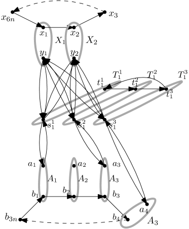
Figure 2: An illustration for Theorem 1.3. The figure shows the part of the construction for a set $S_{1}=\{1,3,4\}$. Dashed arcs denote that there is a cycle through the given vertex whose vertices are not included in the picture. Dark grey bold ellipses denote the sets $V_{i}$.

We claim $I$ has an exact $3$-cover if and only if $x$ is not in the core. “$\Rightarrow$” First suppose $\{S_{k_{1}},\dots,S_{k_{n}}\}$ is an exact $3$-cover in $I$. We claim that $\mathcal{P}=\{A_{i}\mid i\in[3n]\}\cup\{T_{k_{i}}^{l}\mid i\in[n],l\in[3]\}$ is a blocking coalition. We first show that $v(\mathcal{P})=12n$, which can be seen as follows. First, the $s_{j}^{l}$ and $a_{i}$ vertices in the coalition can be covered by $2$-cycles, as the corresponding sets form an exact $3$-cover. Moreover, the $b_{i}$ vertices can be covered by the $b_{i}$-cycle, as each of the $A_{i}$ countries is in $\mathcal{P}$, and finally, the $t_{j}^{l}$ vertices can be covered too, as for each $j\in\{k_{1},\dots,k_{n}\}$ all of $T_{j}^{1},T_{j}^{2},T_{j}^{3}$ belong to $\mathcal{P}$. Then, $x$ is not in the core, as

$$\begin{array}[]{lcl}x(\mathcal{P})&=&3n\cdot(3-\frac{n+1}{9n^{2}})+3n\cdot(1+\frac{1}{9n})\\ &=&9n-\frac{n+1}{3n}+3n+\frac{n}{3n}\\ &<&12n\\ &=&v({\mathcal{P}}).\end{array}$$

“$\Leftarrow$” Now suppose $x$ is not in the core. Then there is a coalition $\mathcal{P}$ with $v(\mathcal{P})>x(\mathcal{P})$. We write $\mathcal{A}=\bigcup_{i\in[3n]}A_{i}$ and $\mathcal{X}=\bigcup_{k\in{6n}}X_{k}$. We claim that $\mathcal{A}\subset\mathcal{P}$ or $\mathcal{X}\subset\mathcal{P}$. For a contradiction, suppose that neither $\mathcal{A}\subset\mathcal{P}$ nor $\mathcal{X}\subset\mathcal{P}$ holds. Clearly, $\mathcal{P}\cap(\mathcal{A}\cup\mathcal{X})\neq\emptyset$, because $m$ of the $T_{j}^{l}$ countries can only create a cycle packing of size $m$, but they each have an allocation of $1+\frac{1}{9n}>1$.

So suppose that $|\mathcal{P}\cap(\mathcal{A}\cup\mathcal{X})|=m\leq 9n$. By our assumption, none of the participating $b_{i}$ or $x_{k}$ vertices can be covered. Hence, if there are $h\geq 1$ participating $T_{j}^{l}$ countries besides them (there must be at least one to have any cycles), then the size of the maximum cycle packing they can obtain is $h+2\min\{m,h\}\leq 2m+h$, as at best all $t_{j}^{l}$ vertices can be covered, but the other vertices can only be covered with cycles of length $2$ by pairing the $h$ $s_{j}^{l}$ vertices to $m$ $a_{i}$ or $x_{i}$ vertices. But, their assigned allocation in $x$ is at least

$$m\cdot\min\{(3-\frac{n+1}{9n^{2}}),(3-\frac{2n-1}{18n^{2}})\}+h\cdot(1+\frac{1}{9n})>2m+h,$$

a contradiction. Hence, $\mathcal{A}\subseteq\mathcal{P}$ or $\mathcal{X}\subseteq\mathcal{P}$ holds.

First suppose that $\mathcal{A}\cup\mathcal{X}\subseteq\mathcal{P}$. Let the number of participating $T_{j}^{l}$ countries be $h$. Then, we have that

$$v(\mathcal{P})\leq 3n+6n+2h+h,\;\mbox{and}$$

$$v(\mathcal{P})>x(\mathcal{P})=18n-\frac{2n-1}{3n}+9n-\frac{n+1}{3n}+h+\frac{h}{9n}.$$

Hence, we find that $2h>18n-1+\frac{h}{9n}>18n-1$, so $h>9n-1$, but it also cannot be $9n$, as $18n=18n-1+\frac{9n}{9n}$, a contradiction (as there are only $9n$ $T_{j}^{l}$ countries).

Suppose next that $\mathcal{X}\subseteq\mathcal{P}$. Let $0\leq m=|\mathcal{P}\cap\mathcal{A}|<3n$. Then, if the number of $T_{j}^{l}$ countries in $\mathcal{P}$ is $h>0$, then $v(\mathcal{P})\leq 6n+h+2\cdot h$. We can suppose that $h\leq 6n+m$, because if there are more $T_{j}^{l}$ countries, then at most $6n+m$ of their $s_{j}^{l}$ vertices can be covered, hence the remaining countries bring strictly more $x$ value than what they can increase the maximum cycle packing size with. However,

$$\begin{array}[]{lcl}x(\mathcal{P})&\geq&(18n-\frac{2n-1}{3n})+(h+\frac{h}{9n})+m\cdot(3-\frac{n+1}{9n^{2}})\\ &>&18n+h+3m-1.\end{array}$$

Hence, in order for $\mathcal{P}$ to block, it must hold that $2h>12n+3m-1$, so $h>6n+1.5m-0.5$, contradicting $h\leq 6n+m$, if $m\geq 1$. In the case, when $m=0$, we get that $6n+3h>18n-\frac{2n-1}{3n}+h+\frac{h}{9n}$, so $2h>12n-\frac{2n-1}{3n}+\frac{h}{9n}>12n-1$. From this and $h\leq 6n+0$, we get that $h$ must be $6n$. However, then $12n>12n-\frac{2n-1}{3n}+\frac{6n}{9n}>12n$, which is a contradiction again.

Therefore, suppose that $\mathcal{A}\subseteq\mathcal{P}$, but $\mathcal{X}$ is not included in $\mathcal{P}$. Let $0\leq m=|\mathcal{P}\cap\mathcal{X}|<6n$. Now, if the number of $T_{j}^{l}$ countries in $\mathcal{P}$ is $h$, then $v(\mathcal{P})\leq 3n+h+2\cdot h$, similarly as before. Again, we can suppose that $h\leq 3n+m$ for similar reasons. Furthermore,

$$\begin{array}[]{lcl}x(\mathcal{P})&\geq&9n-\frac{n+1}{3n}+h+\frac{h}{9n}+m\cdot(3-\frac{2n-1}{9n^{2}})\\ &>&9n+h+3m-1.\end{array}$$

If $m\geq 1$, then this implies that $2h>6n+3m-1$, so $h>3n+1.5m-0.5$, a contradiction. We conclude that $m=0$. Therefore, $h\leq 3n$ and $2h>6n-\frac{n+1}{3n}+\frac{h}{9n}>6n-1$, so $h=3n$.

To sum up, we showed that $\mathcal{P}$ must contain $\mathcal{A}$, must be disjoint from $\mathcal{X}$ and there must be exactly $3n$ $T_{j}^{l}$ countries inside $\mathcal{P}$.

We claim that for each $j\in[3n]$, if $T_{j}^{l}\in\mathcal{P}$ for some $l\in[3n]$, then $T_{j}^{l}$ is inside $\mathcal{P}$ for all $l\in[3]$: if not then there must be at least one $t_{j}^{l}$ vertex that cannot be covered, hence $v(\mathcal{P})\leq 12n-1$, but $x(\mathcal{P})=9n-\frac{n+1}{3n}+3n+\frac{3n}{9n}>12n-1$, a contradiction. Therefore, for each set $S_{j}$, if $T_{j}^{l}\in\mathcal{P}$ for some $l\in[3]$, then $T_{j}^{l}\in\mathcal{P}$ for all $l\in[3]$, so there are exactly $n$ sets $S_{j}$, such that $T_{j}^{l}\in\mathcal{P}$.

Finally, it remains to show that the $n$ sets corresponding to those value of $j$ such that $T_{j}^{l}$ is in $\mathcal{P}$ for $l\in[3]$ must be the indices of an exact $3$-cover. Suppose that there is an element $i$ that cannot be covered by them. Then, $a_{i}$ cannot be covered by a cycle packing by $\mathcal{P}$, so $v(\mathcal{P})\leq 12n-1$, which leads to the same contradiction. ∎

We now prove Theorem 1.4. We need some definitions and a lemma. Let $G=(V,A)$ be a directed graph with a partition $(V_{1},\ldots,V_{n})$ of $V$ for some $n\geq 1$. Recall that for a maximum cycle packing ${\mathcal{C}}$ of $G$, we let $s_{p}({\mathcal{C}})$ denote the number of arcs $(u,v)$ with $v\in V_{p}$ that belong to some directed cycle of ${\mathcal{C}}$. We say that ${\mathcal{C}}$ satisfies a set of intervals $\{I_{1},\ldots,I_{n}\}$ if $s_{p}({\mathcal{C}})\in I_{p}$ for every $p\in\{1,\ldots,n\}$.

Lemma 1

For instances $(G,{\mathcal{V}},{\mathcal{I}})$, where $G$ is a directed graph, ${\mathcal{V}}=(V_{1},\ldots,V_{n})$ is a partition of $V$ with fixed width $c$, and ${\mathcal{I}}=\{I_{1},\dots,I_{n}\}$ is a set of intervals, the problem of finding a maximum cycle packing of $G$ satisfying ${\mathcal{I}}$ is polynomially solvable if $c=1$, and NP-complete if $c\geq 2$ even if $I_{p}=[1,\infty]$ for every $p\in\{1,\ldots,n\}$ or $I_{p}=[1,1]$ for every $p\in\{1,\ldots,n\}$.

Proof

First suppose $c=1$. Let $v_{p}$ be the unique vertex in $V_{p}$. We can assume that each $I_{p}$ contains either $0$ or $1$, else no cycle packing satisfying ${\mathcal{I}}$ exists. If $1\notin I_{p}$, we can delete $v_{p}$ and redefine $G$ as the graph that remains. If this decreases the size of the maximum cycle packing, then we conclude that no desired maximum cycle packing exists. Let $U$ be the set of vertices $v_{p}$ for which $0\notin I_{p}$.

The problem reduces to finding a maximum cycle packing such that each vertex in $U$ is covered. For this, we transform $G=(V,E)$ into a bipartite graph $H$ with partition classes $V$ and $V^{\prime}$, where $V^{\prime}$ is a copy of $V$. For each $v\in V\setminus U$ and its copy $v^{\prime}\in V^{\prime}\setminus U^{\prime}$, we add the edge $uu^{\prime}$ with weight $0$ (we do not add these for the vertices of $U$). For each $(u,v)\in A$, we add the edge $uv$ with weight $1$. It remains to find in polynomial time a maximum weight perfect matching in $H$, if there is any and check whether its weight is the same as the size of a maximum cycle packing in the original directed graph. If there is a perfect matching with that weight, then in the maximum cycle packing it corresponds to, each vertex in $U$ must be covered with a cycle. In the other direction, if there is a maximum cycle packing covering each vertex in $U$, then the perfect matching it corresponds to has the desired weight and we need no nonexistent $uu^{\prime}$ edge for any $u\in U$ indeed.

Now suppose $c\geq 2$. Containment in NP is trivial, as we can easily check if an arc set consists of vertex disjoint cycles or not, and for each county we can compute the number of incoming arcs.

To prove completeness, as in the proof of Theorem 1.3, we reduce from the NP-complete problem Exact $3$-Cover. Given an instance $I$ of Exact $3$-Cover, we construct an instance $I^{\prime}$ of our problem as follows (see also Figure 3):

• For each element $i\in[3n]$, we create a vertex $a_{i}$,

• for each set $S_{j}\in\mathcal{S}$, we create vertices $s_{j}^{1},s_{j}^{2},s_{j}^{3},t_{j}^{1},t_{j}^{2},t_{j}^{3}$,

• we create $2n$ source vertices $x_{1},\dots,x_{2n}$ and $2n$ sink vertices $y_{1},\dots,y_{2n}$.

Define the arcs as follows:

• for each $k\in[2n]$, an arc $(y_{k},x_{k})$,

• for each $k\in[2n],j\in[3n]$, the arcs $(x_{k},t_{j}^{1})$ and $(t_{j}^{3},y_{k})$,

• for each $j\in[3n]$, the arcs $(t_{j}^{1},t_{j}^{2})$ and $(t_{j}^{2},t_{j}^{3})$, and

• for each set $S_{j}=\{j_{1},j_{2},j_{3}\}$, $j_{1}<j_{2}<j_{3}$, the arcs $(s_{j}^{1},a_{j_{1}})$, $(a_{j_{1}},s_{j}^{1})$, $(s_{j}^{2},a_{j_{2}})$, $(a_{j_{2}},s_{j}^{2})$, $(s_{j}^{3},a_{j_{3}})$ and $(a_{j_{3}},s_{j}^{3})$.

This gives a directed graph $G=(V,A)$. We partition $V$ in sets:

• for each $i\in[3n]$, the set $A_{i}=\{a_{i}\}$,

• for each $k\in[2n]$, the sets $X_{k}=\{x_{k}\},Y_{k}=\{y_{k}\}$, and

• for each $j\in[3n],l\in[3]$, $T_{j}^{l}=\{s_{j}^{l},t_{j}^{l}\}$ .

The maximum cycle packing of $G$ has size $16n$. This is because the $x_{i},y_{i}$ vertices allow $2n$ cycles of length $5$ through $t_{j}^{1},t_{j}^{2},t_{j}^{3}$ triples covering $10n$ vertices. The rest of the $t_{j}^{l}$ vertices cannot be covered. Also, for the other $s_{j}^{l}$ and $a_{i}$ vertices, they span a directed bipartite graph, so at most $3n+3n$ vertices can be covered, as we have only $3n$ $a_{i}$ vertices. And $6n$ can be covered indeed, as we can just choose an arbitrary $s_{j}^{l}$ neighbour for each $a_{i}$ and pair them with a 2-cycle.

The interval for each set is $[1,\infty]$. Since the size of the maximum cycle packing of $G$ is $16n$, which is the same as the number of countries, if there is a solution that satisfies these intervals, then it also must satisfy the intervals $[1,1]$ for each set. Hence the last two statements of the Lemma are equivalent in this instance.

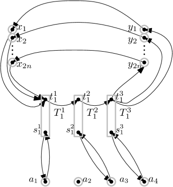
Figure 3: Illustration for Lemma 1, showing the construction for a set $S_{1}=\{1,2,4\}$. Grey bold lines mark the countries.

As a maximum cycle packing in $G$ has size $16n$, which is equal to the sum of the lower bounds, $G$ has a cycle packing satisfying every interval if and only if $G$ has a maximum cycle packing satisfying every interval. We claim $I$ admits an exact $3$-cover if and only if $G$ admits a cycle packing satisfying every interval.

“$\Rightarrow$” First suppose $I$ has an exact $3$-cover $S_{l_{1}},\dots,S_{l_{n}}$. We create a cycle packing $\mathcal{C}$ of $G$. For each $j\in\{l_{1},\dots,l_{n}\}$, we add the cycles $\{(s_{j}^{1},a_{j_{1}}),(a_{j_{1}},s_{j}^{1})\},\{(s_{j}^{2},a_{j_{2}}),(a_{j_{2}},s_{j}^{2})\},\{(s_{j}^{3},a_{j_{3}}),(a_{j_{3}},s_{j}^{3})\}$. For $j\notin\{l_{1},\dots,l_{n}\}$ we add the arcs $(t_{j}^{1},t_{j}^{2}),(t_{j}^{2},t_{j}^{3})$. Finally, for each $i\in[2n]$, we add the arcs $(y_{i},x_{i}),(x_{i},t_{j_{i}}^{1}),(t_{j_{i}}^{3},y_{i})$, where $j_{i}$ is the $i$-th smallest index among the indices $[3n]\setminus\{l_{1},\dots,l_{n}\}$.

Clearly, ${\mathcal{C}}$ is a cycle packing. Each $A_{i}$ has an incoming arc, as $S_{l_{1}},\dots,S_{l_{n}}$ was an exact $3$-cover. As there are exactly $2n$ sets not in the set cover, all of the corresponding sets $T_{j}^{l}$ have one incoming arc in a cycle of the form $\{(y_{i},x_{i}),(x_{i},t_{j_{i}}^{1}),(t_{j_{i}}^{1},t_{j_{i}}^{2}),((t_{j_{i}}^{3},y_{i})\}$, and so did each $X_{i}$ and each $Y_{i}$. Hence, all lower bounds are satisfied.

“$\Leftarrow$” Now suppose $G$ admits a cycle packing satisfying every interval. Then, as $X_{i}$ has an incoming arc for all $i\in[2n]$, all $(x_{i},y_{i})$ arcs are included in the cycle packing. This means that there are $2n$ such $j\in[3n]$, such that the arcs $(t_{j}^{1},t_{j}^{2}),(t_{j}^{2},t_{j}^{3})$ are included in a cycle $\{(y_{i},x_{i}),(x_{i},t_{j}^{1}),(t_{j}^{1},t_{j}^{2}),$ $(t_{j}^{2},t_{j}^{3}),(t_{j}^{3},y_{i})\}$ of $\mathcal{C}$.

From the above, we have that there are $n$ indices $j$ from $[3n]$, such that none of the sets $T_{j}^{1},T_{j}^{2},T_{j}^{3}$ have incoming arcs of this form. Hence, all these sets can only have incoming arcs from a set $A_{i}$. As each such $T_{j}^{i}$ must have one incoming arc, it follows that for all these $j$, the cycles $\{(a_{j_{1}},s_{j}^{1}),(s_{j}^{1},a_{j_{1}})\}$, $\{(a_{j_{2}},s_{j}^{2}),(s_{j}^{2},a_{j_{2}})\}$, $\{(a_{j_{3}},s_{j}^{3}),(s_{j}^{3},a_{j_{3}})\}$ are included in $\mathcal{C}$, so they are vertex disjoint. Hence, the corresponding sets must form an exact $3$-cover. ∎

Theorem 1.4 (restated). For partitioned permutation games even of width $2$, the problem of finding an optimal solution that is weakly or strongly close to a given target allocation $x$ is NP-hard.

Proof

Recall that $x_{p}$ denotes the target for the number of arcs $(u,v)$ with $v\in V_{p}$ that belong to some directed cycle of ${\mathcal{C}}$. Letting each $I_{p}=[x_{p},x_{p}]$ and applying Lemma 1, we see that finding a cycle packing where each $s_{p}({\mathcal{C}})$ is equal $x_{p}$ (so differs by at most $0$) is NP-complete. Thus it is NP-hard to find the maximum cycle packing that minimizes $d_{1}({\mathcal{C}})=\max_{p\in N}\{|x_{p}-s_{p}({\mathcal{C}})|\}$; that is, to find a solution that is weakly close to a given target and similarly it is also hard to find a strongly close solution. ∎

In the remainder of our paper, the following problem plays an important role:

$q$-Exact Perfect Matching
    Instance: An undirected bipartite graph $B=(U,W;E)$, where each edge is coloured with one of $\{1,\dots,q\}$, and numbers $k_{1},\ldots,k_{q}$. Question: Is there a perfect matching in $B$ consisting of $k_{q}$ edges of each colour $q$?

For $q=2$, this problem is also known as Exact Perfect Matching), which, as mentioned, was introduced by Papadimitriou and Yannakakis [32] and whose complexity status is open for more than 40 years. In the remainder of this section, we will gave both a reduction to this problem and a reduction from this problem. We start with doing the former in the proof of our next result (Theorem 2.1), from which Theorem 1.5 immediately follows.

Let $x$ be an allocation for a partitioned permutation game $(N,v)$ on a graph $G=(V,A)$. For a maximum cycle packing ${\mathcal{C}}$, $d^{\prime}({\mathcal{C}})=(|x_{p_{1}}-s_{p_{1}}({\mathcal{C}})|,\dots,|x_{p_{n}}-s_{p_{n}}({\mathcal{C}})|)$ is the unordered deviation vector of ${\mathcal{C}}$.

Theorem 2.1

For a partitioned permutation game $(N,v)$ on a directed graph $G=(V,A)$ and a target allocation $x$, it is possible to generate the set of unordered deviations factors in $|A|^{O(n)}$ time by a randomized algorithm.

Proof

Let $(N,v)$ be a partitioned permutation game with $n$ players, defined on a directed $G=(V,A)$ with vertex partition $V_{1},\ldots,V_{n}$. As mentioned, we reduce from $q$-Exact Perfect Matching for an appropriate value of $q$. From $(N,v)$ and a vector $d^{\prime}=(d_{1}^{\prime},\ldots,d_{n}^{\prime})$ with $d_{p}^{\prime}\geq 0$ for every $p\in N$, we define an undirected bipartite graph $B=(U,W;E)$ with coloured edges: for each vertex $v\in V$, there is a vertex $v^{in}\in U$ and a vertex $v^{out}\in W$ and an edge $v^{in}v^{out}\in E$ that has colour $n+1$; for each arc $(u,v)\in A$, there is an edge $u^{out}v^{in}$, which will be coloured $p$ if $v\in V_{p}$. Let $k_{n+1}=|V|-v(N)$ and, for $p\in\{1,\dots,n\}$, let $k_{p}=d_{p}^{\prime}$.

We observe that $G$ has a maximum cycle packing ${\mathcal{C}}$ with $s_{p}({\mathcal{C}})=d_{p}^{\prime}$ if and only if $B$ has a perfect matching with $k_{p}$ edges of each colour $p\in\{0,\ldots,n\}$.

As each $k_{i}$ can only have a value between $0$ and $|E|=|A|+n=O(|A|)$, the above reduction implies that the set of unordered deviation vectors has size $|A|^{O(n)}$ for any allocation $x$ for $(N,v)$. We can find each of these vectors in $|A|^{O(n)}$ time by a randomized algorithm, as $q$-Exact Perfect Matching is solvable in $|E|^{\mathcal{O}(q)}$ time with $q$ colours with a randomized algorithm [26]. ∎

We cannot hope to derandomize the algorithm from Theorem 2.1 without first solving $2$-Exact Perfect Matching problem in polynomial time. In order to see this, let $B=(U,W;E)$ be a bipartite graph with $|U|=|W|=n$ for some integer $n$ whose edges in $E$ are coloured either red or blue. We construct a digraph $D$ by replacing every edge $e=uv$ with a directed $3$-cycle on arcs $(u,w_{e})$, $(w_{e},v)$, $(v,u)$, where $w_{e}$ is a new vertex that has only $u$ and $v$ as its neighbours in $D$. Let $V_{1}$ consist of all vertices $w_{e}$, for which $e$ is a red edge in $E$. Let $V_{2}=V(D)\setminus V_{1}$. Now, $(B,k,n-k)$ is a yes-instance of $2$-Exact Perfect Matching if and only if $D$ has a cycle packing ${\mathcal{C}}$ with $s_{1}({\mathcal{C}})=k$ and $s_{2}({\mathcal{C}})=3n-k$.

3 ILP Formulation

In this section, we show how to find an optimal solution of a partitioned permutation game that is strongly close to a given target allocation $x$ by solving a sequence of Integer Linear Programs (ILPs). Let $(N,v)$ be a partitioned permutation game defined on a directed graph $G=(V,A)$. Recall that for a maximum cycle packing ${\mathcal{C}}$ of $G$, we let $s_{p}({\mathcal{C}})$ denote the number of arcs $(u,v)$ with $v\in V_{p}$ that belong to some directed cycle of ${\mathcal{C}}$. Recall also that $|x_{p}-s_{p}({\mathcal{C}})|$ is the deviation of country $p\in N$ from its target $x_{p}$ if ${\mathcal{C}}$ is chosen as optimal solution. Moreover, in the vector $d({\mathcal{C}})=(|x_{p_{1}}-s_{p_{1}}({\mathcal{C}})|,\dots,|x_{p_{n}}-s_{p_{n}}({\mathcal{C}})|)$, the deviations $|x_{p}-s_{p}({\mathcal{C}})|$ are ordered non-increasingly. Finally, we recall that ${\mathcal{C}}$ is strongly close to $x$ if $d({\mathcal{C}})$ is lexicographically minimal over all optimal solutions for $(N,v)$.

In the kidney exchange literature the following ILP is called the edge-formulation (see e.g. [1]) For each $a\in A$, let $e_{a}\in\{0,1\}$ be a binary edge-variable for $D$.

$$\begin{array}[]{rl}M^{*}:=\displaystyle\max_{e}\sum_{ij\in A}e_{ij}&\text{s.t.}\\[-5.0pt] \end{array}$$ (edge-formulation)

$$\begin{array}[]{rclr}\displaystyle\sum_{j:ji\in A}e_{ji}&=&\displaystyle\sum_{j:ij\in A}e_{ij}&\forall i\in V\\ \displaystyle\sum_{j:ji\in A}e_{ji}&\leq&1&\forall i\in V\\ \end{array}$$

The first set of constraints represents the (well-known) Kirchoff law. The second set of constraints ensures that every node is covered by at most one cycle. The objective function provides a maximum cycle packing (of size $M^{*}$).

This ILP has $|A|$ binary variables and $2|V|$ constraints. In the following we are going to sequentially find largest country deviations $d_{t}^{*}$ ($t\geq 1$) and the corresponding minimal number $n_{t}^{*}$ of countries receiving that deviation. We achieve this by solving one ILP of similar size for each $d_{t}^{*}$ and $n_{t}^{*}$, so two ILPs per iteration $t$. By similar size, we mean that in each iteration we are going to add $|N|$ binary variables and a single additional constraint, while $|N|\leq|V|$ holds by definition and typically $|N|$ is much smaller than $|A|$. Meanwhile, since at every iteration we are going to fix the deviation of at least one additional country (we will not necessarily know which country, we are only going to keep track of number of countries with fixed deviation), the number of iterations are at most $|N|$ (as $t\leq|N|$). Hence, we will solve no more than $2|N|$ ILPs, among which the largest has $\mathcal{O}(|A|+|N|^{2})$ binary variables and $\mathcal{O}(|V|+|N|)=\mathcal{O}(|V|)$ constraints.

Once we have $M^{*}$ we solve the following ILP to find $d_{1}^{*}$:

$$\begin{array}[]{rl}d_{1}^{*}:=\displaystyle\min_{e,d_{1}}d_{1}&\text{s.t.}\\ \end{array} \text{ILP}_{d_{1}}$$ ()

$$\begin{array}[]{rclr}\displaystyle\sum_{j:ji\in A}e_{ji}&=&\displaystyle\sum_{j:ij\in A}e_{ij}&\forall i\in V\\[18.0pt] \displaystyle\sum_{j:ji\in A}e_{ji}&\leq&1&\forall i\in V\\[18.0pt] \displaystyle\sum_{ij\in A}e_{ij}&=&M^{*}&\\[18.0pt] \displaystyle\sum_{j\in V_{p}}e_{ij}-x_{p}&\leq&d_{1}&\forall p\in N\\[18.0pt] \displaystyle x_{p}-\sum_{j\in V_{p}}e_{ij}&\leq&d_{1}&\forall p\in N\end{array}$$

The first three constraints guarantee that all solutions are in fact maximum cycle-packings. These constraints will be part of the formulation throughout the entire ILP-series. The remaining two constraints, together with the objective function guarantees that we minimize the largest country deviation. Note that for each country $p$, exactly one of $\sum_{j\in V_{p}}e_{ij}-x_{p}$ and $x_{p}-\sum_{j\in V_{p}}e_{ij}$ is positive and exactly one of them is negative, unless both of them are zero. However, as soon as we reach $d_{t}^{*}\leq 1/2$ we have found a strongly close maximum cycle-packing. Hence, in the remainder, we assume $d_{t}^{*}>1/2$ for each $t$ such that the series continues with $t+1$.

($\text{ILP}_{d_{1}}$) has one additional continuous variable ($d_{1}$) and $2|N|+1$ additional constraints. For every country $p\in N$ we have that $|\sum_{j\in V_{p}}e_{ij}-x_{p}|\leq d_{1}^{*}$. However, there exists a smallest subset $N_{1}\subseteq N$ (which may not necessarily be unique) such that

$$\begin{array}[]{ll}\displaystyle\left|\sum_{j\in V_{p}}e_{ij}-x_{p}\right|=d_{1}^{*}&\forall p\in N_{1}\\ &\\ \displaystyle\left|\sum_{j\in V_{p}}e_{ij}-x_{p}\right|\leq d_{2}^{*}<d_{1}^{*}&\forall p\in N\setminus N_{1}\end{array}$$

In a solution of ($\text{ILP}_{d_{1}}$), let $n_{1}$ be the number of countries with deviation $d_{1}^{*}$. We need to determine if there is another solution of ($\text{ILP}_{d_{1}}$) with fewer than $n_{1}$, possibly $n_{1}^{*}$, countries having $d_{1}^{*}$ deviation. For this purpose we must be able to distinguish between countries unable to have less than $d_{1}^{*}$ deviation and countries for which the deviation is at most $d_{2}^{*}$, the latter value unknown at this stage. In order to make this distinction, we determine a lower bound on $d_{1}^{*}-d_{2}^{*}$ by examining the target allocation $x$. We will then set $\varepsilon$ in the next ILP to be strictly smaller than this lower bound.

The number of vertices for a country covered by any cycle-packing is an integer. Hence, the number of possible country deviations is at most $2|N|$ and depends only on $x$. The fractional part of a country deviation is either $\operatorname{frac}(x_{p})$ or $1-\operatorname{frac}(x_{p})$. Therefore, to find the minimal positive difference in between the deviations of any two countries $p$ and $q$, we have to compare the values $\operatorname{frac}(x_{p})$ and $1-\operatorname{frac}(x_{p})$, with $\operatorname{frac}(x_{q})$ or $1-\operatorname{frac}(x_{q})$ and take the minimum of those four possible differences. Let $\varepsilon$ be a small positive constant that is strictly smaller than the minimum possible positive difference between any two countries.

We will distinguish between countries having minimal deviation of $d_{1}^{*}$ and others through additional binary variables. Since later in the ILP series we will need to distinguish between countries fixed at different deviation levels, let us introduce $z^{t}_{p}\in\{0,1\}$ binary variables, where $z^{t}_{p}=1$ indicates that $p\in N_{t}$.

$$\begin{array}[]{rl}\displaystyle\min_{z^{1},e}\displaystyle\sum_{p\in N}z^{1}_{p}&\text{s.t.}\\ \end{array} \text{ILP}_{N_{1}}$$ ()

$$\begin{array}[]{rclr}\displaystyle\sum_{j:ji\in A}e_{ji}&=&\displaystyle\sum_{j:ij\in A}e_{ij}&\forall i\in V\\ \displaystyle\sum_{j:ji\in A}e_{ji}&\leq&1&\forall i\in V\\ \displaystyle\sum_{ij\in A}e_{ij}&=&M^{*}&\\ \displaystyle\sum_{j\in V_{p}}e_{ij}-x_{p}&\leq&d_{1}^{*}-\varepsilon(1-z^{1}_{p})&\forall p\in N\\ \displaystyle x_{p}-\sum_{j\in V_{p}}e_{ij}&\leq&d_{1}^{*}-\varepsilon(1-z^{1}_{p})&\forall p\in N\end{array}$$

As discussed, for each country $p$, the left hand side of either the fourth or the fifth constraint is negative (i.e., would be satisfied even with $z^{1}_{p}=0$). For those countries whose deviation cannot be lower than $d_{1}^{*}$, however, the (positive) left hand side of either the fourth or the fifth constraint will require $z^{1}_{p}=1$. Thus, given an optimal solution $z^{1*}$ of ($\text{ILP}_{N_{1}}$), let $n_{1}^{*}:=\sum_{p\in N}z_{p}^{1*}$ be the minimal number of countries receiving the largest country deviations. It is guaranteed that the non-increasingly ordered country deviations at a strongly close maximum cycle packing starts with exactly $n_{1}^{*}$ many $d_{1}^{*}$ values, followed by some $d_{2}^{*}<d_{1}^{*}$. ($\text{ILP}_{N_{1}}$) has $|A|+|N|$ binary variables and $2|V|+2|N|+1$ constraints. Now, to find $d_{2}^{*}$, we solve the following ILP:

$$\begin{array}[]{rl}\displaystyle\min_{d_{2},e,z^{1}}d_{2}&\text{s.t.}\\ \end{array} \text{ILP}_{d_{2}}$$ ()

$$\begin{array}[]{rclr}\displaystyle\sum_{j:ji\in A}e_{ji}&=&\displaystyle\sum_{j:ij\in A}e_{ij}&\forall i\in V\\ \displaystyle\sum_{j:ji\in A}e_{ji}&\leq&1&\forall i\in V\\ \displaystyle\sum_{ij\in A}e_{ij}&=&M^{*}&\\ \displaystyle\sum_{j\in V_{p}}e_{ij}-x_{p}&\leq&d_{1}^{*}&\forall p\in N\\ \displaystyle x_{p}-\sum_{j\in V_{p}}e_{ij}&\leq&d_{1}^{*}&\forall p\in N\\ \displaystyle\sum_{j\in V_{p}}e_{ij}-x_{p}&\leq&d_{2}+z^{1}_{p}d_{1}^{*}&\forall p\in N\\ \displaystyle x_{p}-\sum_{j\in V_{p}}e_{ij}&\leq&d_{2}+z^{1}_{p}d_{1}^{*}&\forall p\in N\\ \displaystyle\sum_{p\in N}z^{1}_{p}&=&n_{1}^{*}&\end{array}$$

($\text{ILP}_{d_{2}}$) has $|A|+|N|$ binary variables and one continuous variable ($d_{2}$) with $2|V|+4|N|+2$ constraints, and guarantees that we find the minimal second-largest country deviation $d_{2}^{*}$ while exactly $n_{1}^{*}$ countries deviation is kept at $d_{1}^{*}$. Finding $n_{2}^{*}$ follows a similar approach, where $L$ is a large constant satisfying $L\geq 2(d_{1}^{*}-d_{2}^{*})$:

$$\begin{array}[]{rl}\displaystyle\min_{z^{1},z^{2},e}\displaystyle\sum_{p\in N}z^{2}_{p}&\text{s.t.}\\ \end{array} \text{ILP}_{N_{2}}$$ ()

$$\begin{array}[]{rclr}\displaystyle\sum_{j:ji\in A}e_{ji}&=&\displaystyle\sum_{j:ij\in A}e_{ij}&\forall i\in V\\ \displaystyle\sum_{j:ji\in A}e_{ji}&\leq&1&\forall i\in V\\ \displaystyle\sum_{ij\in A}e_{ij}&=&M^{*}&\\ \displaystyle\sum_{j\in V_{p}}e_{ij}-x_{p}&\leq&d_{2}^{*}-\varepsilon(1-z^{2}_{p})+z_{p}^{1}L&\forall p\in N\\ \displaystyle x_{p}-\sum_{j\in V_{p}}e_{ij}&\leq&d_{2}^{*}-\varepsilon(1-z^{2}_{p})+z_{p}^{1}L&\forall p\in N\\ \displaystyle\sum_{j\in V_{p}}e_{ij}-x_{p}&\leq&d_{1}^{*}&\forall p\in N\\ \displaystyle x_{p}-\sum_{j\in V_{p}}e_{ij}&\leq&d_{1}^{*}&\forall p\in N\\ \displaystyle\sum_{p\in N}z^{1}_{p}&=&n_{1}^{*}&\\ z_{p}^{1}+z_{p}^{2}&\leq&1&\forall p\in N\end{array}$$

Subsequently we follow a similar approach for all $t\geq 3$, until either $|N|=n_{1}^{*}+n_{2}^{*}+\dots+n_{t}^{*}$ or we terminate because $d_{t}^{*}\leq 1/2$. Until reaching one of these conditions we iteratively solve the following two ILPs, introducing additional $|N|$ binary variables and an additional constraint to both. Let $L$ be a large constant satisfying $L\geq d_{t}^{*}$, e.g. $L=d_{t-1}^{*}$.

$$\begin{array}[]{rl}\displaystyle\min_{d_{t},e,(z^{i})_{i=1}^{t-1}}d_{t}&\text{s.t.}\\ \end{array} \text{ILP}_{d_{t}}$$ ()

$$\begin{array}[]{rclr}\displaystyle\sum_{j:ji\in A}e_{ji}&=&\displaystyle\sum_{j:ij\in A}e_{ij}&\forall i\in V\\ \displaystyle\sum_{j:ji\in A}e_{ji}&\leq&1&\forall i\in V\\ \displaystyle\sum_{ij\in A}e_{ij}&=&M^{*}&\\ \displaystyle\sum_{i=1}^{t-1}z^{i}_{p}&\leq&1&\forall p\in N\\ \displaystyle\sum_{j\in V_{p}}e_{ij}-x_{p}&\leq&d_{t}+\displaystyle\sum_{i=1}^{t-1}z^{i}_{p}d_{i}^{*}&\forall p\in N\\ \displaystyle x_{p}-\sum_{j\in V_{p}}e_{ij}&\leq&d_{t}+\displaystyle\sum_{i=1}^{t-1}z^{i}_{p}d_{i}^{*}&\forall p\in N\\ \displaystyle\sum_{j\in V_{p}}e_{ij}-x_{p}&\leq&\displaystyle\sum_{i=1}^{t-1}z^{i}_{p}d_{i}^{*}+(1-\displaystyle\sum_{i=1}^{t-1}z^{i}_{p})L&\forall p\in N\\ \displaystyle x_{p}-\sum_{j\in V_{p}}e_{ij}&\leq&\displaystyle\sum_{i=1}^{t-1}z^{i}_{p}d_{i}^{*}+(1-\displaystyle\sum_{i=1}^{t-1}z^{i}_{p})L&\forall p\in N\\ \displaystyle\sum_{p\in N}z^{i}_{p}&=&n_{i}^{*}&\forall i=1,\dots,t-1\end{array}$$

In the following formulations $L$ is a large constant satisfying $L\geq d_{t}^{*}-\varepsilon$.

$$\begin{array}[]{rl}\displaystyle\min_{(z)_{i=1}^{t},e}\displaystyle\sum_{p\in N}z^{t}_{p}&\text{s.t.}\\ \end{array} \text{ILP}_{N_{t}}$$ ()

$$\begin{array}[]{rclr}\displaystyle\sum_{j:ji\in A}e_{ji}&=&\displaystyle\sum_{j:ij\in A}e_{ij}&\forall i\in V\\ \displaystyle\sum_{j:ji\in A}e_{ji}&\leq&1&\forall i\in V\\ \displaystyle\sum_{ij\in A}e_{ij}&=&M^{*}&\\ \displaystyle\sum_{i=1}^{t}z^{i}_{p}&\leq&1&\forall p\in N\\ \displaystyle\sum_{j\in V_{p}}e_{ij}-x_{p}&\leq&d_{t}^{*}-\varepsilon(1-z^{t}_{p})+\displaystyle\sum_{i=1}^{t-1}z_{p}^{i}d_{i}^{*}&\forall p\in N\\ x_{p}-\displaystyle\sum_{j\in V_{p}}e_{ij}&\leq&d_{t}^{*}-\varepsilon(1-z^{t}_{p})+\displaystyle\sum_{i=1}^{t-1}z_{p}^{i}d_{i}^{*}&\forall p\in N\\ \displaystyle\sum_{j\in V_{p}}e_{ij}-x_{p}&\leq&\displaystyle\sum_{i=1}^{t}z_{p}^{i}d_{i}^{*}+(1-\displaystyle\sum_{i=1}^{t}z_{p}^{i})L&\forall p\in N\\ \displaystyle x_{p}-\sum_{j\in V_{p}}e_{ij}&\leq&\displaystyle\sum_{i=1}^{t}z_{p}^{i}d_{i}^{*}+(1-\displaystyle\sum_{i=1}^{t}z_{p}^{i})L&\forall p\in N\\ \displaystyle\sum_{p\in N}z^{i}_{p}&=&n_{i}^{*}&\forall i=1,\dots,t-1\end{array}$$

From the above, we conclude that the following theorem holds.

Theorem 3.1

For a partitioned permutation games $(N,v)$ defined on a graph $G=(V,A)$, it is possible to find an optimal solution that is strongly close to a given target allocation $x$ by solving a series of at most $2|N|$ ILPs, each having $O(|A|+|N|^{2})$ binary variables and $O(|V|)$ constraints.

Note that if we just want to find a weakly close optimal solution we can stop after solving the first ILP.

4 Simulations

In this section we describe our simulations for $\ell=\infty$ in detail. Our goals are

1. to examine the benefits of strongly close optimal solutions over weakly close optimal solutions or arbitrary chosen optimal solutions when $\ell=\infty$;

2. to examine benefits of using credits when $\ell=\infty$;

3. to examine the exchange cycle length distribution when $\ell=\infty$; and

4. to compare the results for $\ell=\infty$ with the known results [8] for the other extreme case when $\ell=2$.

For our fourth aim, we want to know in particular how much scope there is for improvement in the total number of kidneys when we move from $\ell=2$ to $\ell=\infty$.

Set Up. To do a fair comparison we follow the same set up as in [8], and in addition, we also use the data from [6] that was used in [8]. That is, for our simulations, we take the same 100 compatibility graphs $G_{1},\ldots,G_{100}$, each with roughly 2000 vertices from [6, 8]. As real medical data is unavailable to us for privacy reasons, the data from [6, 8] was obtained by using the data generator from [33]. This data generator was used in many papers and is the most realistic synthetic data generator available; see also [23].

For every $i\in\{1,\ldots,100\}$ we do as follows. For every $n\in\{4,\ldots,10\}$, we perform simulations for $n$ countries. We first partition $V(G_{i})$ into the same $n$ sets $V_{i,1},\ldots,V_{i,n}$ as in [8] of equal size ${2000}/{n}$ (subject to rounding), so $V_{i,p}$ is the set of patient-donor pairs of country $p$. For round 1, we construct a compatibility graph $G_{i}^{1}$ as a subgraph of $G_{i}$ of size roughly $500$. We add the remaining patient-donor pairs of $G_{i}$ as vertices by a uniform distribution between the remaining rounds.

Starting with $G_{i}^{1}(n)$ we run a IKEP of 24 rounds in total. This gives us 24 compatibility graphs $G_{i}^{1}(n),\ldots,G_{i}^{24}(n)$. Just as in [8], any patient-donor pair, whose patient is not helped within four rounds, will be automatically deleted from the pool.

A (24-round) simulation instance consists of the data needed to generate a graph $G_{i}^{1}(n)$ and its successors $G_{i}^{2}(n),\ldots,G_{i}^{24}(n)$, together with specifications for the choice of initial allocation and optimal solution (maximum cycle packing). Our code for obtaining the simulation instances is in GitHub repository [42], along with the compatibility graphs data and the seeds for the randomization.

We now discuss our choice for the initial allocations and optimal solutions (maximum cycle packings).

Initial allocations. For the initial allocations $y$ we use the Banzhaf value, Shapley value, nucleolus, benefit value and contribution value. The Shapley value $\phi(N,v)$ [36] is defined by $\phi_{p}(N,v)=\sum_{S\subseteq N\backslash\{p\}}\frac{|S|!(n-|S|-1)!}{n!}(v(S\cup\{p\})-v(S))$. To define the next solution concept, we first introduce unnormalized Banzhaf value $\psi_{p}(N,v)$ [30] defined by $\psi_{p}(N,v):=\sum_{S\subseteq N\backslash\{p\}}\frac{1}{2^{n-1}}(v(S\cup\{p\})-v(S))$. As $\psi_{p}$ may not be an allocation, the (normalized) Banzhaf value $\overline{\psi}_{p}(N,v)$ of a game $(N,v)$ was introduced and defined by $\overline{\psi}_{p}(N,v):=\frac{\psi_{p}(N,v)}{\sum_{q\in N}\psi_{q}(N,v)}\cdot v(N)$. Whenever we mention the Banzhaf value, we will mean $\overline{\psi}(N,v)$. For the Shapley value and Banzhaf value, we were still able to implement a brute force approach relying on the above definitions.

We now define the nucleolus. The excess for an allocation $x$ of a game $(N,v)$ and a non-empty coalition $S\subsetneq N$ is defined as $e(S,x):=x(S)-v(S)$. Ordering the $2^{n}-2$ excesses in a non-decreasing sequence yields excess vector $e(x)\in\mathbb{R}^{2^{n}-2}$. The nucleolus of a game ($N,v$) is the unique allocation [35] that lexicographically maximizes $e(x)$ over the set of allocations $x$ with $x_{i}\geq v(\{i\})$ (assuming this set is nonempty, as holds in our case). To compute the nucleolus, we use the Lexicographical Descent method of [10], which is the state-of-the-art method in nucleolus computation.

The surplus of a game $(N,v)$ is $\mbox{surp}=v(N)-\sum_{p\in N}v(\{p\})$. One can allocate $v(\{p\})+\alpha_{p}\cdot\mbox{surp}$, as long as $\sum_{p\in N}\alpha_{p}=1$, to a player $p\in N$. If $\alpha_{p}=\frac{v(N)-v(N\setminus\{p\})-v(\{p\})}{\sum_{p\in N}(v(N)-v(N\setminus\{p\})-v(\{p\}))}$, we obtain the benefit value. If $\alpha_{p}=\frac{v(N)-v(N\setminus\{p\})}{\sum_{p\in N}(v(N)-v(N\setminus\{p\}))}$, we get the contribution value. Both values are easy to compute, but may not exist if the denominator is zero, which did not happen in our simulations.

Optimal solutions. We compute weakly and strongly close optimal solutions by solving a sequence of ILPs, as described in Section 3. We used g++ version 11 on Ubuntu 20.04 for our C++ implementation. The values $v(S)$ of the partitioned permutation games used in the ILPs are obtained by solving a maximum weight perfect matching problem (see Section 1), for which we use the package of [24].

Computational environment and scale. We run our simulations both without and with (“$+c$”) using the credit system, and for the settings, where an arbitrary optimal solution (“arbitrary”), weakly optimal solution (“$d_{1}$”) or strongly optimal optimal solution (“lexmin”) is chosen. This leads to the following five scenarios for each of the five selected solution concepts, the Shapley value, nucleolus, Banzhaf value, benefit value and contribution value: arbitary, d1, d1+c, lexmin, and lexmin+c. Note that for the arbitrary scenario, the use of credits is irrelevant. Hence, in total, we run the same set of simulations for $5\times 5=25$ different combinations of scenarios and initial allocations. As we have seven different country sizes $n$ and 100 initial compatibility graphs $G_{i}$, our total number of 24-round simulation instances is $25\times 7\times 100=17500$.

All simulations were run on a dual socket server with Xeon Gold 6238R processors with 2.2 GHz base speed and 512GB of RAM, where each simulation was given eight cores and 16GB of RAM.

Evaluation measures. Let $y^{*}$ be the total target allocation of a single simulation instance, i.e., $y^{*}$ is obtained by taking the sum of the 24 initial allocations of each of the 24 rounds. Let ${\mathcal{C}}^{*}$ be the union of the chosen maximum cycle packings in each of the 24 rounds. We use the total relative deviation defined as $\frac{\sum_{p\in N}|y_{p}^{*}-s_{p}({\mathcal{C}^{*}})|}{|{\mathcal{C}^{*}}|}$. For each choice of initial allocation and choice of scenario, we run 100 instances. We take the average of the 100 relative total deviations to obtain the average total relative deviation. Taking the maximum relative deviation $\frac{\max_{p\in N}|y_{p}^{*}-s_{p}({\mathcal{C}^{*}})|}{{\mathcal{C}^{*}}}$ gives us the average maximum relative deviation as our second evaluation measure. As we shall see, this evaluation measure leads to the same conclusions.

Simulation Results for ${\mathbf{\ell=\infty}}$ and Comparison with ${\mathbf{\ell=2}}$. In Figure 4 we display our main results. In this figure, we compare different solutions concepts under different scenarios for $\ell=\infty$. The figure also shows the effects of weakly and strongly close solutions and the credit system. As solution concepts have different complexities, we believe such a comparison might be helpful for policy makers for choosing a solution concept and scenario. As expected, using an arbitrary maximum cycle packing in each round makes the kidney exchange scheme significantly more unbalanced, with average total relative deviations over 4% for all initial allocations $y$. The effect of both selecting a strongly close solution (to ensure being close to a target allocation) and using a credit function (for fairness, to keep deviations small) is significant.

The above observations are in line with the results under the setting where $\ell=2$ [8]. However, for $\ell=2$, the effect of using arbitrary optimal solutions is worse, while deviations are smaller than for $\ell=\infty$ when weakly close or strongly close optimal solutions are chosen. From Figure 4 we see that the Shapley value and the Banzhaf value in the lexmin+c scenario provide the smallest deviations from the target allocations (just like when $\ell=2$ [8]). However, differences are small and, as mentioned, which solution concept to select is up to the policy makers of the IKEP. Moreover, from Figure 4, we can also see the benefits of $\ell=\infty$ over $\ell=2$ for the Shapley value.

Figure 5 shows that if we use the average maximum relative deviation instead of the average total relative deviation, then we can see the same pattern as in Figure 4.

From Figure 6 we see that when $\ell=\infty$ instead of $\ell=2$, it is possible to achieve 46% more kidney transplants. The $\ell=\infty$ setting is not realistic. Namely, Figure 7 show that long cycles, with even more than 400 vertices, may occur. Figure 7 also shows that these long cycles all happen in the first round. We note that before our experiments, the relation between increase in transplants versus increase in cycle length had not been researched by simulations. Finding out about this was our main motivation for our simulations.

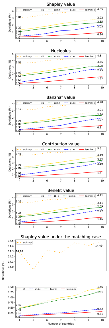
Figure 4: Average total relative deviations for each of the five solution concepts under the five different scenarios, where the number of countries $n$ is ranging from $4$ to $10$. For comparison, the bottom figure displays a result from [8] for $\ell=2$, namely for the Shapley value, which behaved best for $\ell=2$.

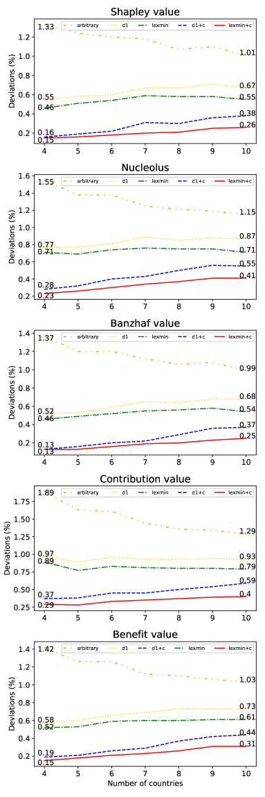
Figure 5: Average maximum relative deviations for each of the five solution concepts under the five different scenarios, where the number of countries $n$ is ranging from $4$ to $10$.

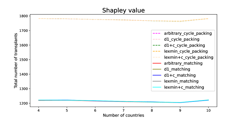
Figure 6: The total number of kidney transplants when the Shapley value is chosen, both when $\ell=2$ (five scenarios, with overlapping plots) and when $\ell=\infty$ (five scenarios, with overlapping plots). The number of countries $n$ is ranging from $4$ to $10$.

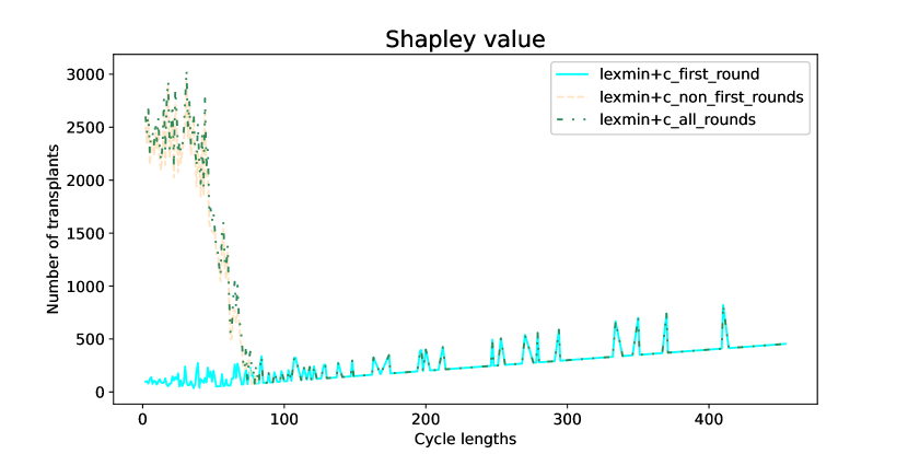
Figure 7: Cycle distribution for the Shapley value in the lexmin+c scenario, where the x-axis represents the cycle length, and the y-axis shows the number of kidney transplants involved in a cycle of that length.

5 Conclusions

We introduced the class of partitioned permutation games and proved a number of complexity results that contrast known results for partitioned matching games. Our new results guided our simulations for IKEPs with up to ten countries, with exchange bound $\ell=\infty$. Our simulations showed a significant improvement in the total number of kidney transplants over the case where $\ell=2$ [8] at the expense of long cycles. In our simulations, all countries had the same size. In [8], simulations were also done for countries with three different sizes, but these led to the same conclusions. We expect the same for $\ell=\infty$, as confirmed by a robustness check for $n=6$ (see Github repository [42]).

For future research we will consider the more realistic exchange bounds $\ell\in\{3,4,5\}$. We note that the simulations done in [11, 31] were only for $\ell=3$; a more limited number of solution concepts; for IKEPs with up to four countries; and only for scenarios that use weakly close optimal solutions. They also used different data sets. For our follow-up study for $\ell\in\{3,4,5\}$, we must now also overcome, just like [11, 31], the additional computational obstacle of not being able to compute an optimal solution for a compatibility graph in a KEP round and the values $v(S)$ of the associated permutation game in polynomial time (see Theorem 1.1). Current techniques for $\ell\in\{3,4,5\}$ therefore involve, besides ILPS based on the edge-formulation, ILPs based on the cycle-formulation, with a variable for each cycle of length at most $\ell$ (see, for example, [20, 22, 25]). Hence, computing a single value $v(S)$ will become significantly more expensive, and even more so for increasing $\ell$. For expensive solution concepts, such as the Shapley or nucleolus, we must compute an exponential number of values $v(S)$. Without any new methods, we expect it will not be possible to do this for simulations up to the same number of countries (ten) as we did for $\ell=\infty$.

Finally, we note that matching games and permutation games are usually defined on edge-weighted graphs. It is readily seen that all our positive theoretical results can be generalized to this setting. In kidney exchange, the primary goal is still to help as many patients as possible, but edge weights might be used to represent transplant utilities. Hence, it would also be interesting to do simulations in the presence of edge weights. We leave this as future research.

Acknowledgments. Benedek was supported by the National Research, Development and Innovation Office of Hungary (OTKA Grant No. K138945); Biró by the Hungarian Scientific Research Fund (OTKA, Grant No. K143858) and the Hungarian Academy of Sciences (Momentum Grant No. LP2021-2); Csáji by the Hungarian Scientific Research Fund (OTKA Grant No. K143858) and the Momentum Grant of the Hungarian Academy of Sciences (Grant No. 2021-1/2021); and Paulusma was supported by the Leverhulme Trust (Grant RF-2022-607) and EPSRC (Grant EP/X01357X/1). Moreover, this work has used Durham University’s NCC cluster. NCC has been purchased through Durham University’s strategic investment funds, and is installed and maintained by the Department of Computer Science. In particular, we thank Rob Powell for his help with setting up our simulations on the NCC cluster.

References

- [1] Abraham, D.J., Blum, A., Sandholm, T.: Clearing algorithms for barter exchange markets: enabling nationwide kidney exchanges. Proceedings EC 2007 pp. 295–304 (2007)
- [2] Ashlagi, I., Fischer, F., Kash, I.A., Procaccia, A.D.: Mix and match: A strategyproof mechanism for multi-hospital kidney exchange. Games and Economic Behavior 91, 284 – 296 (2015)
- [3] Ashlagi, I., Roth, A.E.: New challenges in multihospital kidney exchange. American Economic Review 102, 354–359 (2012)
- [4] Ashlagi, I., Roth, A.E.: Free riding and participation in large scale, multi-hospital kidney exchange. Theoretical Economics 9, 817–863 (2014)
- [5] Aziz, H., Cseh, Á., Dickerson, J.P., McElfresh, D.C.: Optimal kidney exchange with immunosuppressants. Proceedings AAAI 2021 pp. 21–29 (2021)
- [6] Benedek, M.: International kidney exchange scheme (2021), https://github.com/blrzsvrzs/int_kidney_exchange
- [7] Benedek, M., Biró, P., Johnson, M., Paulusma, D., Ye, X.: The complexity of matching games: A survey. Journal of Artificial Intelligence Research 77, 459–485 (2023)
- [8] Benedek, M., Biró, P., Kern, W., Paulusma, D.: Computing balanced solutions for large international kidney exchange schemes. Proceedings AAMAS 2022 pp. 82–90 (2022)
- [9] Benedek, M., Biró, P., Paulusma, D., Ye, X.: Computing balanced solutions for large international kidney exchange schemes. CoRR abs/2109.06788 (2023)
- [10] Benedek, M., Fliege, J., Nguyen, T.: Finding and verifying the nucleolus of cooperative games. Mathematical Programming 190, 135–170 (2021)
- [11] Biró, P., Gyetvai, M., Klimentova, X., Pedroso, J.P., Pettersson, W., Viana, A.: Compensation scheme with Shapley value for multi-country kidney exchange programmes. Proceedings ECMS 2020 pp. 129–136 (2020)
- [12] Biró, P., Haase-Kromwijk, B., Andersson, T., et al.: Building kidney exchange programmes in Europe – an overview of exchange practice and activities. Transplantation 103, 1514–1522 (2019)
- [13] Biró, P., Kern, W., Pálvölgyi, D., Paulusma, D.: Generalized matching games for international kidney exchange. Proceedings AAMAS 2019 pp. 413–421 (2019)
- [14] Biró, P., Klijn, F., Klimentova, X., Viana, A.: Shapley-scarf housing markets: Respecting improvement, integer programming, and kidney exchange. Mathematics of Operations Research to appear (2023)
- [15] Biró, P., Manlove, D.F., Rizzi, R.: Maximum weight cycle packing in directed graphs, with application to kidney exchange programs. Discrete Mathematics, Algorithms and Applications 1, 499–518 (2009)
- [16] Blum, A., Caragiannis, I., Haghtalab, N., Procaccia, A.D., Procaccia, E.B., Vaish, R.: Opting into optimal matchings. Proceedings SODA 2017 pp. 2351–2363 (2017)
- [17] Böhmig, G.A., Fronek, J., Slavcev, A., Fischer, G.F., Berlakovich, G., Viklicky, O.: Czech-Austrian kidney paired donation: first european cross-border living donor kidney exchange. Transplant International 30, 638–639 (2017)
- [18] Carvalho, M., Lodi, A.: A theoretical and computational equilibria analysis of a multi-player kidney exchange program. European Journal of Operational Research 305, 373–385 (2023)
- [19] Carvalho, M., Lodi, A., Pedroso, J.a.P., Viana, A.: Nash equilibria in the two-player kidney exchange game. Mathematical Programming 161, 389–417 (2017)
- [20] Constantino, M., Klimentova, X., Viana, A., Rais, A.: New insights on integer-programming models for the kidney exchange problem. European Journal of Operational Research 231, 57–68 (2013)
- [21] Curiel, I.J., Tijs, S.H.: Assignment games and permutation games. Methods of Operations Research 54, 323–334 (1986)
- [22] Delorme, M., García, S., Gondzio, J., Kalcsics, J., Manlove, D., Pettersson, W.: New algorithms for hierarchical optimisation in kidney exchange programmes. Operations Research (to appear)
- [23] Delorme, M., García, S., Gondzio, J., Kalcsics, J., Manlove, D.F., Pettersson, W., Trimble, J.: Improved instance generation for kidney exchange programmes. Computers & Operations Research 141, 105707 (2022)
- [24] Dezso, B., Jüttner, A., Kovács, P.: LEMON - an open source C++ graph template library. Proceedings WGT@ETAPS, Electronic Notes in Theoretical Computer Science 264, 23–45 (2010)
- [25] Dickerson, J.P., Manlove, D.F., Plaut, B., Sandholm, T., Trimble, J.: Position-indexed formulations for kidney exchange. Proceedings of EC 2016 pp. 25–42 (2016)
- [26] Gurjar, R., Korwar, A., Messner, J., Straub, S., Thierauf, T.: Planarizing gadgets for perfect matching do not exist. Proceedings MFCS 2012, Lecture Notes in Computer Science 7464, 478–490 (2012)
- [27] Hajaj, C., Dickerson, J.P., Hassidim, A., Sandholm, T., Sarne, D.: Strategy-proof and efficient kidney exchange using a credit mechanism. Proceedings AAAI 2015 pp. 921–928 (2015)
- [28] Hein, J., Jiang, T., Wang, L., Zhang, K.: On the complexity of comparing evolutionary trees. Discrete Applied Mathematics 71, 153–169 (1996)
- [29] Hickey, G., Dehne, F., Rau-Chaplin, A., Blouin, C.: Spr distance computation for unrooted trees. Evolutionary Bioinformatics 4, EBO–S419 (2008)
- [30] III, J.F.B.: Weighted voting doesn’t work: A mathematical analysis. Rutgers Law Review 19, 317–343 (1964)
- [31] Klimentova, X., Viana, A., Pedroso, J.a.P., Santos, N.: Fairness models for multi-agent kidney exchange programmes. Omega 102, 102333 (2021)
- [32] Papadimitriou, C.H., Yannakakis, M.: The complexity of restricted spanning tree problems. Journal of the ACM 29, 285–309 (1982)
- [33] Pettersson, W., Trimble, J.: Kidney matching tools data set generator (2021), https://wpettersson.github.io/kidney-webapp/#/generator
- [34] Roth, A.E., Sönmez, T., Ünver, M.U.: Kidney exchange. Quarterly Journal of Economics 119, 457–488 (2004)
- [35] Schmeidler, D.: The nucleolus of a characteristic function game. SIAM Journal on Applied Mathematics 17, 1163–1170 (1969)
- [36] Shapley, L.S.: A value for -person games. Annals of Mathematical Studies 28, 307–317 (1953)
- [37] Smeulders, B., Blom, D., Spieksma, F.C.R.: Identifying optimal strategies in kidney exchange games is -complete. Mathematical Programming to appear (2022)
- [38] Sun, Z., Todo, T., Walsh, T.: Fair pairwise exchange among groups. Proceedings IJCAI 2021 pp. 419–425 (2021)
- [39] Tijs, S., Parthasarathy, T., Potters, J.A., Prassad, V.R.: Permutation games: another class of totally balanced games. OR Spektrum 6, 119–123 (1984)
- [40] Toulis, P., Parkes, D.C.: Design and analysis of multi-hospital kidney exchange mechanisms using random graphs. Games and Economic Behavior 91, 360–382 (2015)
- [41] Valentín, M.O., Garcia, M., Costa, A.N., Bolotinha, C., Guirado, L., Vistoli, F., Breda, A., Fiaschetti, P., Dominguez-Gil, B.: International cooperation for kidney exchange success. Transplantation 103, 180–181 (2019)
- [42] Ye, X.: International kidney exchange data (2023), https://github.com/Arya1531/international_kidney_exchange_program/tree/main