Surojit Ganguli, Zeyu Zhou, Christopher G. Brinton, David I. Inouye
Purdue University
West Lafeyette
{sganguli,zhou1059,cgb,dinouye}email@purdue.edu

Fault-Tolerant Vertical Federated Learning on Dynamic Networks

Surojit Ganguli, Zeyu Zhou, Christopher G. Brinton, David I. Inouye
Purdue University
West Lafeyette
{sganguli,zhou1059,cgb,dinouye}email@purdue.edu

Abstract

Vertical Federated learning (VFL) is a class of FL where each client shares the same sample space but only holds a subset of the features. While VFL tackles key privacy challenges of distributed learning, it often assumes perfect hardware and communication capabilities. This assumption hinders the broad deployment of VFL, particularly on edge devices, which are heterogeneous in their in-situ capabilities and will connect/disconnect from the network over time. To address this gap, we define Internet Learning (IL) including its data splitting and network context and which puts good performance under extreme dynamic condition of clients as the primary goal. We propose VFL as a naive baseline and develop several extensions to handle the IL paradigm of learning. Furthermore, we implement new methods, propose metrics, and extensively analyze results based on simulating a sensor network. The results show that the developed methods are more robust to changes in the network than VFL baseline.

1 Introduction

In recent times, Federated Learning (FL) has emerged as a popular approach to distributed machine learning when data is distributed across clients. FL was primarily developed with the goal of data privacy and efficient communication McMahan et al., (2017). FL has two standard approaches based on the method of partitioning of data among parties: horizontal (which is the most common) and vertical. The data context in horizontal FL (HFL) involves each client possessing unique samples of the full set of features, while Vertical FL (VFL) involves each party sharing the same set of samples while only possessing a portion of the features Wu et al., (2022). The focus for the research presented here is the VFL context.

An ideal VFL scenario involves synchronous aggregation of client models at the server. However, due to communication and computation heterogeneity commonly associated with FL setups – attributed to dynamic changes to the network of clients – in practice the condition for VFL implementation is anything but ideal. Below, we highlight some real-world use cases of VFL where the data is distributed across clients but the system’s ability to handle dynamic changes to the network of clients is critical (e.g., performance under near catastrophic faults).

Use-case 1: Precision Agriculture In recent times, modernization of agriculture has been aided by the adoption of sensor networks to aid with high crop yield Thakur et al., (2019). Within individual farms, each sensor will collect measurements on a portion of the crops (i.e., a subset of the features in VFL), making their individual measurements important to the global models. Yet the sensors may become unreliable given harsh outdoor conditions. Thus, sensors may leave or join the network arbitrarily. System performance must be reliable even in such a scenario.

Use-Case 2: Social-based recommender systems Tech companies employ user data for ad recommendations and entertainment suggestions, but privacy concerns threaten the sustainability of centralized systems. Customers want personalized predictions within trusted circles, with each user possessing a subset of the information (i.e., VFL features) on the influence of recommendation decisions. This private network operates without a central server, allowing users to join or leave based on privacy concerns.

While client faults have been studied in HFL (see subsection 1.1), literature on making VFL robust under dynamic network changes is sparse. Unlike HFL, which involves averaging model parameters, VFL involves concatenating model outputs from different clients, making it more challenging to assure robustness under dynamic network conditions. Some emerging works have considered VFL dynamics, e.g., Li et al., (2023) studied asynchronous clients and Chen et al., (2020) studied straggler clients. However, prior works on fault-tolerant VFL assume there is a special server node that does not fault, and only consider train-time faults. No prior works consider VFL with both train-time and test-time faults where any node can fail.

To fill this gap, we introduce the Internet Learning (IL) paradigm that aims to achieve strong performance under dynamic network conditions, particularly extreme changes, where the features of the data samples are distributed across clients as in VFL.

Owing to its widespread adoption and desirable characteristics such as data privacy, we suggest VFL be used as a baseline and propose several natural extensions of VFL to handle the more challenging context of IL. We consider performance in dynamic scenarios, including near catastrophic faults and nodes joining, as the primary metric for assessing algorithms developed for IL setup. A comparison of IL with federated learning paradigms is captured in Figure 1. We summarize our contributions as follows:

• We define the context and goal of Internet Learning (IL). The context of IL assumes the features are split across clients while the communication network is dynamic, allowing for both communications and devices to fault. We define the goal of IL as minimizing the IL risk, which measures performance under (extreme) dynamic network conditions.

• We propose several modifications of VFL to handle the challenging IL problem including replication of the server nodes, multiple layers of replicated VFL, and gossip-based layers.

• We implement a scalable and modular experimental testbed for IL using the abstraction of message passing to enable reproducible and systematic evaluation protocols for IL.

• We evaluate our IL methods under ideal and dynamic conditions for multiple datasets. Our results demonstrate that VFL fairs unfavorably when dealing with train and test time network faults while our proposed methods are more robust to faults.

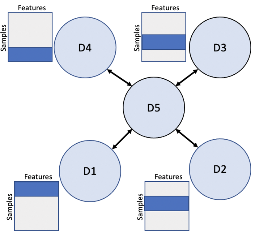
(a) Horizontal FL

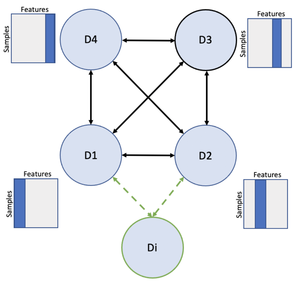
(b) Internet Learning (IL)

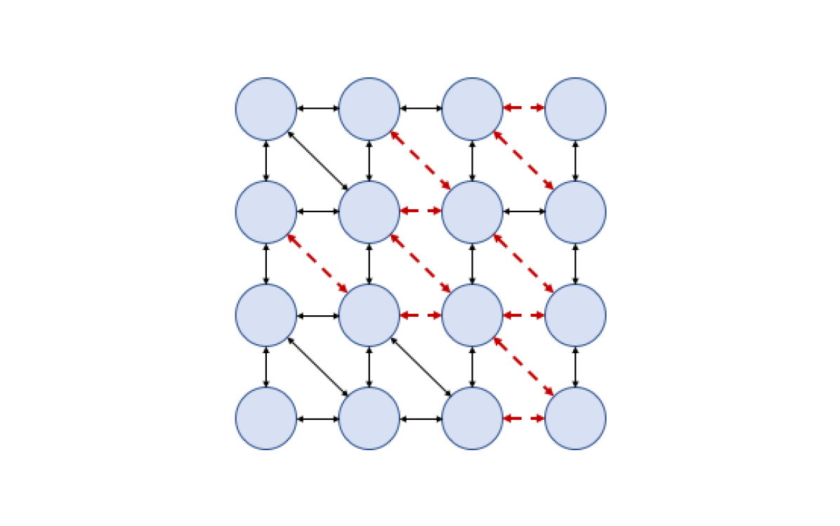
(c) Network faults in IL

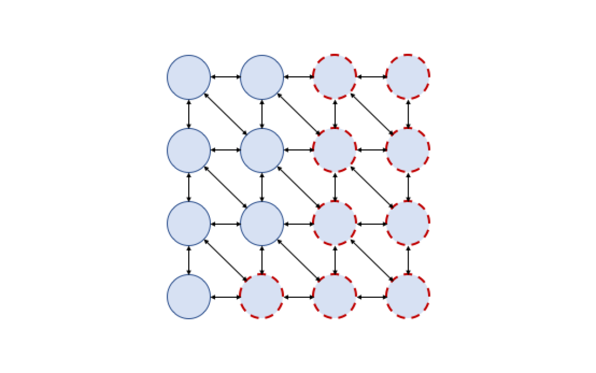
(d) Device faults in IL

Figure 1: While standard (Horizontal) FL assumes samples are split across clients 1(a) with a central server, the data context of IL is the same as Vertical FL where the features are split across clients but where no centralized server node is assumed and clients can leave or join 1(b). Importantly, IL aims to perform well even under highly dynamic networks such as near catastrophic (e.g., 50%) communication 1(c) and device 1(d) faults (shown in red) during both the training and testing. Because of the VFL data context of features split across devices 1(b), network faults mean both a loss of feature values and a loss of computation.

1.1 Related works

Asynchronous and Straggler-Resilient FL

Network dynamics have received attention in HFL. Wang and Ji, (2022) studied the problem of arbitrary client participation and provided an unified convergence analysis under this non-ideal condition. Gu et al., (2021) proposed MIFA, which alleviates device straggler challenges by memorizing the latest updates from devices. Ruan et al., (2021) considers flexible client participation during the training process and proposes aggregation scheme that provides convergence guarantees even in such a scenario. (Liu et al.,, 2021; Chen et al.,, 2021; van Dijk et al.,, 2020) have studied protocols to handle asynchronous client updates. While these HFL methods may provide inspiration, they do not match our feature-split VFL context and thus are not directly applicable. In the VFL context, Chen et al., (2020); Zhang et al., (2021); Li et al., (2020) studied the problem of asynchronous client participation with the objectives of reducing the communication cost, accelerating training, and accounting for device heterogeneity. Li et al., (2023) noted that asynchronous VFL protocols lead to staleness of model updates, resulting in performance degradation, and proposed FedVS which utilizes secret sharing of data and model parameters among clients to introduce redundancy. However, these VFL methods are focused on train-time faults, while our primary focus is performance under test-time faults.

Decentralized FL

Other works in the HFL setting have considered decentralized network architectures, i.e., networks of clients without an aggregation server. Tang et al., (2022) developed GossipFL that uses gossip learning to achieve communication efficient-training, and obtains comparable performance to central HFL. Lalitha et al., (2019) leverages peer to peer learning to achieve HFL in a decentralized manner. Feng et al., (2021) proposed a Blockchain-based decentralized HFL framework. Although gossip based and peer to peer learning based methods are viable options for decentralized HFL, they are not, by themselves, considered reliable when network conditions are dynamic Gabrielli et al., (2023). Nonetheless, we borrow some ideas from gossip-based protocols in our proposed methods.

2 Problem Formulation

Internet Learning specifies both an operating context and the desired properties of a learning system. The context is comprised of two entities: the data context and the network context, which we define in the first subsection. The desired property of the system is robustness under dynamic conditions, which we formally define via IL risk and corresponding metrics in the next two subsections. The term “Internet Learning” was inspired by packet switching, which forms the backbone of the internet. Specifically, packet switching communication networks were designed to perform well even under near catastrophic faults (e.g., major nuclear war) (Baran,, 1964). While these catastrophic faults have not occurred in practice, the design principle of extreme robustness produced an entirely new approach to communication networks. Therefore, IL aims for performance even under extreme conditions.

Notation

Let $\mathcal{X}=\{\bm{x}_{i}\}_{i=1}^{n}$ denote a dataset of with $n$ samples and $d$ features. Let $\bm{x}_{\mathcal{S}}$ denote the subvector associated with the indices in $\mathcal{S}\subseteq\{1,2,\cdots,d\}$, e.g., if $\mathcal{S}=\{1,5,8\}$, then $\bm{x}_{\mathcal{S}}=[x_{1},x_{5},x_{8}]^{T}$. For $C$ clients, the dataset at each client $c\in\{1,2,\cdots,C\}$ will be denoted by $\mathcal{X}_{c}$. Let $\mathcal{G}=(\mathcal{C},\mathcal{E})$ denote a network (or graph) of clients, where $\mathcal{C}\subseteq\{1,2,\cdots,C\}$ denotes the clients and $\mathcal{E}$ denotes the communication edges.

2.1 Internet Learning Context

In this section, we define the data context and the network context for IL. First, we define the partial features data context and then discuss the dynamic network assumption.

Definition 1 (Partial Features Data Context).

A partial features data context means that each client has access to a subset of the features, i.e., $\mathcal{X}_{c}=\{\bm{x}_{i,\mathcal{S}_{c}}\}_{i=1}^{n},$ where $\mathcal{S}_{c}\subset\{1,2,\cdots,d\}$ for each client $c$.

This is the same data context as VFL but we use generic terminology because the network context, assumptions, and applicable methods may differ from the standard VFL setup. One example of this VFL data context is the setup wherein data for the same patient is distributed across multiple hospitals and there is little to no overlap in the data among the hospitals. Another key example is a sensor network where each sample is based on timestamps, i.e., each sensor observes a partial part of the environment but the same time as other sensors. Furthermore, in this study we assume that the features with each client is a partition of the feature set of a sample and each client has disjoint set of features for each sample. However, we do allow for scenarios where the clients can have features among one another that are correlated. For instance, there can be two sensors that can have correlated features due to their physical proximity.

Definition 2 (Dynamic Network Context).

A dynamic network means that the communication graph can change across time indexed by $t$, i.e., $\mathcal{G}(t)=(\mathcal{C}(t),\mathcal{E}(t))$, where the changes over time can be either deterministic or stochastic functions of $t$.

This dynamic network context includes many possible scenarios including various network topologies, clients joining or leaving the network, and communication being limited or intermittent due to power constraints or physical connection interference. We provide two concrete dynamic models where there are device failures or communication failures. For simplicity, we will assume there is a base network topology $\mathcal{G}_{\mathrm{base}}=(\mathcal{C}_{\mathrm{base}},\mathcal{E}_{\mathrm{base}})$ (e.g., complete graph, grid graph or preferential-attachment graph), and we will assume a discrete-time version of a dynamic network where $t\in\{0,1,2,\cdots\}$. Given this, we can formally define two simple dynamic network models that encode random device and communication faults.

Definition 3 (Device Fault Dynamic Network).

Given a fault rate $p$ and a baseline topology $\mathcal{G}_{\mathrm{base}}$, a device fault dynamic network $\mathcal{G}_{\mathrm{DF}}(t)$ means that a client is in the network at time $t$ with probability $1-p$, i.e., $\mathrm{Pr}(c\in\mathcal{C}_{\mathrm{DF}}(t))=1-p,\forall c\in\mathcal{C}_{\mathrm{base}}$ and $\mathcal{E}_{\mathrm{DF}}(t)=\{(c,c^{\prime})\in\mathcal{E}_{\mathrm{base}}:c,c^{\prime}\in\mathcal{C}_{\mathrm{DF}}(t)\}$.

Definition 4 (Communication Fault Dynamic Network).

Given a fault rate $p$ and a baseline topology $\mathcal{G}_{\mathrm{base}}$, a communication fault dynamic network $\mathcal{G}_{\mathrm{CF}}(t)$ means that a communication edge (excluding self-communication) is in the network at time $t$ with probability $1-p$, i.e., $\mathcal{C}_{\mathrm{CF}}(t)=\mathcal{C}_{\mathrm{base}}$ and $\mathrm{Pr}((c,c^{\prime})\in\mathcal{E}_{\mathrm{CF}}(t))=1-p,\forall(c,c^{\prime})\in\mathcal{E}_{\mathrm{base}}$ where $c\neq c^{\prime}$.

As this work focuses on the foundations of IL, we only experimented with these two dynamic network models. However, more complex dynamic models could be explored in the future. For example, the networks could change smoothly over time (e.g., one connection being removed or added at every time point. Or, a network could model a catastrophic event at a particular time $t^{\prime}$ followed by a slow recovery of the network as devices are reconnected or restarted. We leave the investigation of more complex dynamic models to future work.

2.2 Internet Learning Problem

Given these context definitions, we now define the goal of IL in terms of the IL risk which we define next. For now, we will assume the existence of a distributed inference algorithm $\Psi(\bm{x};\theta,\mathcal{G}(t))$ that can predict across the data-split network under the dynamic conditions given by $\mathcal{G}(t)$. In subsection 2.3, we will explain our generic distributed inference algorithm that generalizes VFL that will be used in our methods and that formalizes our proposed metrics.

Definition 5 (Internet Learning Risk).

Assuming the partial features data context (1) and given a dynamic network $\mathcal{G}(t)$ (2), the internet learning risk of all clients’ parameters denoted by $\theta$ is defined as the expected test loss $\ell$ when evaluated with the dynamic network: $R_{\mathcal{G}(t)}(\theta)\triangleq\mathbb{E}_{(\bm{x},y)\sim p_{\mathrm{test}}}[\ell(\Psi(\bm{x};\theta,\mathcal{G}(t)),y)]\,,$ where $\Psi$ is a distributed inference algorithm and $p_{\mathrm{test}}$ is the test distribution.

We will use the term “system” or “network” instead of “model” as all computation must be computed in a distributed manner. This means that the network’s parameters $\theta$ are distributed across all clients. We also note that the model at each client could have different parameters and even different architectures, unlike in HFL.

Given this risk definition, we can now fully define the internet learning problem.

Definition 6 (Internet Learning Problem).

Given partial features client datasets $\{\mathcal{X}_{c}\}_{c=1}^{C}$ (Definition 1) and a dynamic network $\mathcal{G}(t)$ (Definition 2), the internet learning problem aims to find the optimal client parameters $\theta$ that minimize the IL risk $R_{\mathcal{G}(t)}$ under the constraint that $\theta$ are the outputs of some distributed learning algorithm $\Omega(\{\mathcal{X}_{c}\}_{c=1}^{C},\mathcal{G}(t))$, i.e.,

$$\begin{aligned} \min_{\theta}\quad R_{\mathcal{G}(t)}(\theta)\text{ s.t. }\quad\theta=\Omega(\{\mathcal{X}_{c}\}_{c=1}^{C},\mathcal{G}^{\prime}(t)),\end{aligned}$$ (1)

where $\mathcal{G}^{\prime}(t)$ is a dynamic (possibly stochastic) network used during training.

Like the significant change from circuit switching to packet switching, we expect that algorithms may have to be completely redesigned to work on extreme dynamic networks that are not present in standard centralized learning paradigms.

2.3 Distributed Inference Algorithm

While the distributed inference algorithm $\Psi(\bm{x};\theta,\mathcal{G}(t))$ could be any distributed algorithm in theory, we focus on a particular type of distributed inference algorithm based on message passing rounds. In particular, we assume that the distributed inference algorithm alternates between local computation on the client and message passing between clients. For the test phase, the final communication round is between the clients and an external entity that will use the prediction. As examples, the external entity could represent a drone passing over a remote sensing network to gather predictions or a physical connection to the devices at test time (e.g., when the sensors are ultra-low power and cannot directly connect to the internet). Or, this external entity could represent a power intensive connection via satellite to some base station that would only activate when requested to save power. We will first define the intermediate representations of the network computation and then define the final communication layer to accommodate for different scenarios.

For our definition of the algorithm, let $\bm{x}_{c}$ denote the features at client $c$ for an input $\bm{x}$, which represents the concatenated features across the whole network. Let $\bm{z}_{c}^{(t)}$ denote the representation at time $t$ for client $c$.

Definition 7 (Message Passing Inference Algorithm).

The message passing distributed inference algorithm $\Psi$ is defined as follows:

$$\Psi(\bm{x};\theta,\mathcal{G}(\cdot)) \triangleq h(\bm{z}_{1}^{(T)},\bm{z}_{2}^{(T)},\cdots,\bm{z}_{C}^{(T)};\mathcal{G}(T))$$ (2)

where $h$ represents the final communication to an external entity, $\mathcal{G}(t)$ includes a special node indexed by 0 representing the external entity, and the latent representation $\bm{z}_{c}^{(t)}$ for times $1\leq t\leq T$ for all clients $c\in\mathcal{C}(t)$ is the combination of local computation and message passing:

$$\bm{z}_{c}^{(1)} \triangleq f_{c}^{(1)}(\bm{x}_{c};\theta_{c}^{(1)})$$ (3)

$$\bm{z}_{c}^{(t)} \triangleq f_{c}^{(t)}\big{(}g(\{\bm{z}_{c^{\prime}}^{(t-1)}:(c,c^{\prime})\in\mathcal{E}(t)\});\theta_{c}^{(t)}\big{)},\forall t>1$$

where $f_{c}^{(t)}$ is a model with parameters $\theta_{c}^{(t)}$ and $g$ is an aggregation function over neighbor messages.

While this functional form has a superficial resemblance to the computation in graph neural networks (GNN), there are important semantic and syntactic differences, which we discuss in the appendix. In practice, we take $g$ to concatenate the received messages while putting zeros for messages not received. This choice directly generalizes simple VFL pipelines, which use latent feature concatenation. Now we will define the final processing function $h$ which represents the communication to the external entity. We consider two practical scenarios and two oracle methods that provide upper and lower bounds on the best and worst performance depending on how $h$ selects the final output of the inference algorithm. These four methods for defining $h$ will enable the computation of IL risk under different scenarios and form the basis for the four test metrics in the experimental section. For these, we will assume that $h$ produces $C$ class predictions for each client, i.e., $h:\mathbb{R}^{C\times m}\to\{0,1,2,\cdots,m\}^{C}$, where $m$ is the number of classes, so we can define $\hat{\bm{y}}\triangleq h(\bm{z}_{1},\cdots,\bm{z}_{c};\mathcal{G})$. We will then define the loss function as the number of correct answers over the number of non-zero values, where zero represents a missing prediction. The main difference is how to aggregate the predictions under faults (or in VFL where only 1 node acts as the server and computes the classification prediction).

Average Over Clients

If it can be assumed that all clients can communicate their outputs to the external entity (e.g., they can all communicate with a drone that passes by), then a natural measure is the average accuracy over all clients that successfully communicate to this external entity (i.e., the device does not fault and the communication does not fault):

$$\hat{\bm{y}}_{c}^{\mathrm{avg}}\triangleq\begin{cases}\operatorname*{arg\,max\,}_{i}\bm{z}_{i,c},&\text{if }c\in\mathcal{C}(T),(c,0)\in\mathcal{E}(T)\\ 0,&\text{otherwise}\,.\end{cases}$$

where the $0$-th client represents the external entity and a $0$ output means that the device faulted and therefore does not provide any prediction (and will not be counted in the denominator of the loss).

Furthermore, if all devices produce 0, then we randomly sample a class prediction (e.g., if the server fails in VFL).

Random Client Prediction

A slightly different case is the prediction at a device is chosen at random. This models the case where only a single device can communicate with the external entity (e.g., via a physical connection created at test time to extract information from a remote sensing grid). For this definition, let $\mathrm{Cat}(a)$ represents a random sample from a categorical distribution with $a$ categories. Given a random client $c^{\prime}\sim\mathrm{Cat}(C)$, the random client prediction zero for all clients $c\neq c^{\prime}$ and the following for the randomly selected client $c^{\prime}$:

$$\hat{\bm{y}}_{c^{\prime}}^{\mathrm{rand}} \triangleq\begin{cases}\operatorname*{arg\,max\,}_{i}\bm{z}_{i,c^{\prime}},&\text{if }c^{\prime}\in\mathcal{C}(T),(c^{\prime},0)\in\mathcal{E}(T)\\ \mathrm{Cat}(m),&\text{otherwise}\end{cases}$$

Oracle Best and Worst Client Prediction

Finally, we provide two bounds on selecting the best and worst client when doing prediction. These are oracle because they require access to the true label $y$ to select the right client. The oracle best and worst client prediction can be defined as:

$$\hat{\bm{y}}_{c}^{\mathrm{best}} \triangleq\operatorname*{arg\,max\,}_{\bm{y}^{\mathrm{avg}}_{c^{\prime}}:c^{\prime}\in\mathcal{C}(t)}\bm{1}(\bm{y}^{\mathrm{avg}}_{c^{\prime}}=y),\forall c\in\mathcal{C}(t)$$

$$\hat{\bm{y}}_{c}^{\mathrm{worst}} \triangleq\operatorname*{arg\,min\,}_{\bm{y}^{\mathrm{avg}}_{c^{\prime}}:c^{\prime}\in\mathcal{C}(t)}\bm{1}(\bm{y}^{\mathrm{avg}}_{c^{\prime}}=y),\forall c\in\mathcal{C}(t)$$

where $\bm{y}^{\mathrm{avg}}_{c^{\prime}}$ is the average output defined above and $\bm{1}(a=b)$ is an indicator function that is one if $a=b$. Intuitively, if any non-faulted client prediction is correct, we predict the true label for oracle best. Similarly, for oracle worst, if any non-faulted client prediction is incorrect, we predict the wrong label. The worst case lower bounds a single client prediction, i.e., the system’s accuracy even if the worst client is selected.

3 Proposed IL Methods

Here we explain baseline and newly proposed methods that can be used in the IL paradigm. Figure 2 summarizes the different proposed methods and contrasts it with the baseline. Unless mentioned otherwise, learning is taking place in all the represented layers, $L_{t}$, which represent the $f_{c}^{(t)}$ functions. As mentioned in Section 1, owing to the similarity in regards to the data context, VFL seems to be a natural fit as a baseline. In the VFL setup , there is a single server and multiple clients. This can be represented by the clients in the network in the second round is only the server node, i.e., $\mathcal{C}(2)=\{c_{\mathrm{server}}\}$. For experiments that will be presented in the paper, in VFL, one of the participating clients is randomly chosen as the server.

Multiple VFL

Given the critical role that the server has, if the communication to server were to be lost or the server faults out, the learning will be ineffective. In order to prevent such a catastrophic failure, we propose Multiple VFL (MVFL), which is a straightforward extension of the VFL setup to multiple servers. In MVFL, all the participating clients act as servers.

Deep MVFL

Extending the MVFL setup, we propose another variant, Deep MVFL (DMVFL), which stacks MVFL models on top of each other and necessitates multiple rounds of communication between devices for each input. We believe that multiple communication rounds and deeper processing could lead to more robustness on dynamic networks. Comparing Figure 2 (b) and (c), the setup is same till $L_{2}$ but in DMVFL, there is an additional round of communication in $L_{3}$ following which the predictions are made. In Figure 2 (c) we have illustrated DMVFL with just one additional round of communication over MVFL and hence the depth of DMVFL is 1. Nonetheless, the depth in DMVFL need not be restricted to 1 and is a hyperparameter. Furthermore, to guarantee a fair comparison between DMVFL and MVFL, it was ensured that the number of parameters for both these setups be the same.

Output Gossip Layers

Finally, we also propose gossip (G) based method. Hegedűs et al., (2019) demonstrated that gossip learning is a viable alternative to federated learning and aggregating model parameters from peers eliminates the need for a central server. Taking inspiration from this finding, we believe that gossiping the penultimate output across all devices can lead to more robust methods. In Figure 2 (d) MVFL-G refers to the gossip variant of MVFL where the log probability outputs of each client are averaged using a round of gossip passing, which can be viewed as a fixed averaging layer that does not have parameters.

For instance in Figure 2 (d) the latent representations at output of $L_{2}$ (penultimate layer) for $D_{1}$ and $D_{2}$ are averaged together and used as inputs for $L_{3}$ (last layer) from which the predictions are made. In the sample setup, averaging is performed once. However, the number of times averaging can be performed is a hyperparameter. It is critical to note that in the methods proposed here, the gossip protocol is that of averaging log probabilities and does not involve any learning. Nonetheless, it is possible to incorporate intricate learnable gossip protocols. Following a similar logic a gossip variant for DMVFL, DMVFL-G can also be formulated.

(a) VFL

(b) MVFL

(c) DMVFL

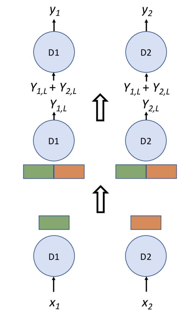
(d) MVFL-G

Figure 2: VFL as a baseline and the proposed methods are illustrated for a network of two fully connected devices, D1 and D2. (a)VFL setup with D1 acting as a client as well as the aggregating server. The input to the devices at the first layer $L_{1}$ are $x_{1}$ and $x_{2}$ and output are the latent representations. The input to the server on the second layer $L_{2}$ is the concatenated latent representation and the output is the prediction $y_{1}$ (b) MVFL arrangement has both the devices acting as servers aside from being clients. (c) DMVFL has a similar arrangement as MVFL, expect that there is an additional layer of processing, $L_{3}$, that has the concatenated features from the previous layer as an input and the output are the predictions. (d) MVFL-G is an extension of MVFL wherein the output log probabilities ($Y_{i,L}$) from each device are averaged before being used for final prediction.

4 Experiments

In this section, we compare of our proposed methods and with the baseline VFL across diverse scenarios. Our primary focus is to assess the advantages of incorporating multiple servers, introducing additional rounds of communication among servers, and leveraging a final phase of gossip communication. This exploration is aimed at enhancing the resilience of our distributed machine learning system for different baseline networks, fault patterns, and fault rates during training and inference.

Subsequently, we delve into a more meticulous investigation, with a specific emphasis on understanding how the number of communication rounds in DMVFL, as well as the frequency of gossip communication in MVFL and DMVFL, influence the model’s performance.

4.1 Experimental Setup

Dataset

We test with MNIST, StarCraftMNIST (Kulinski et al.,, 2023), and CIFAR10. Due to space constraint, results with StarCraftMNIST are presented here and findings with other datasets are in the Appendix. We chose StarCraftMNIST as it is specifically designed to study different tasks over a sensor network, which matches with the context described in the use-cases (Section 1). The results presented below consider 16 clients. In the Appendix we provide analysis with other datasets for different number of clients. Depending on the number of clients chosen, each client obtains different features for a given sample. In case of 16 clients, we first split StarCraftMNIST images into a 4x4 square grid of patches. This splits a 28x28 image into 16 patches, each sized 7x7, with one patch assigned to each client. For other datasets, the procedure is similar.

Methods

As discussed in Section 3, the following methods are studied. 1) VFL: Out of the 16 clients, one of the clients is randomly chosen as the server and it is responsible for prediction; 2) MVFL: All the sixteen clients function as server and each is capable of providing a prediction; 3) DMVFL: Similar setup as MVFL with additional rounds of communication. The additional rounds are denoted by D$i$. For example D2 implies 2 additional rounds of communication; 4) MVFL-G or DMVFL-G: The $i$ in G$i$ denotes the number of rounds of message aggregation at the penultimate layer. Specifics about model architecture and and training parameters can be found in the Appendix. In the main paper, we use geometric averaging for the gossiping as it is more standard, and in the appendix, we do a more careful study of different gossiping methods.

Baseline Communication Network

We consider two types: Complete or Grid. In the former all the clients are connected to the server and in the latter only the neighboring clients, decided based on a distance metric, are connected. Details regarding the implementation of the metric and how it is used to generate the Grid network can be found in the Appendix. For any experiment, a communication network is first chosen and different fault patterns are then applied to that chosen network.

Fault Models

We investigate models’ performance under two different dynamic network scenarios: device faults and communication faults defined in Definition 3 and Definition 4, respectively. Note that these device and communication faults could affect the final communication to the external entity, e.g., if the server in VFL faults, then the external entity does not does not receive a prediction. For simplicity, we assume that the communication graph is constant for processing an entire batch (including the backward pass during training). Future work could consider a streaming setting in which the communication graph could change while a batch is being processed.

For implementing faults, we will investigate five different fault rates for both types of faults (0$\%$, 10$\%$, 20$\%$, 30$\%$, 40$\%$, 50$\%$). In the situation a communication or device is faulted out, we impute the missing values with zeros and assume that for training or inference. In the experiments we use a batch size of 64. Given there are two different communication networks and fault patterns, we run experiments with the following combinations: complete-device, complete-communication, grid-deviceand grid-communication.For its practical purposefulness, "Average Performance" is chosen as the metric in which the results in the section below are presented.

4.2 Result

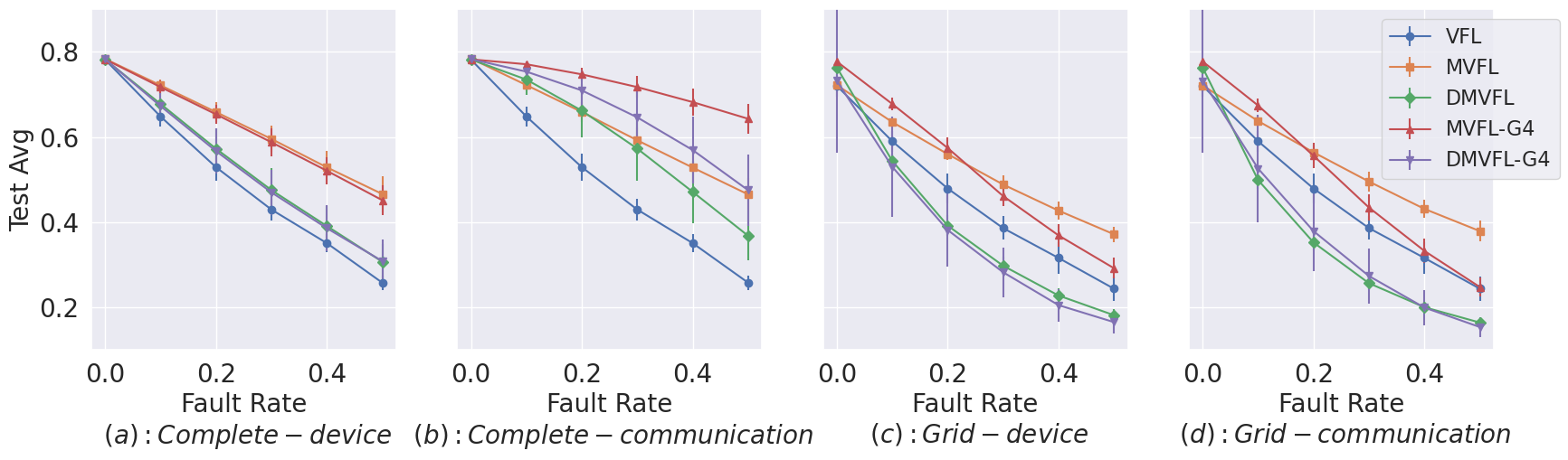
Figure 3: Test average accuracy under no train fault and different test time fault rates for StarCraftMNIST with 16 devices. All results are averaged over 16 runs and error bar represents standard deviation. Observing (a),(b),(c),(d) it can be concluded that VFL does not do well under different faulting conditions. Furthermore, in complete network (a),(b) MVFL when employed with 4 rounds of gossiping leads to the most robust average performance. For grid network, (c),(d), it’s either MVFL or MVFL-G4 that has the best performance.

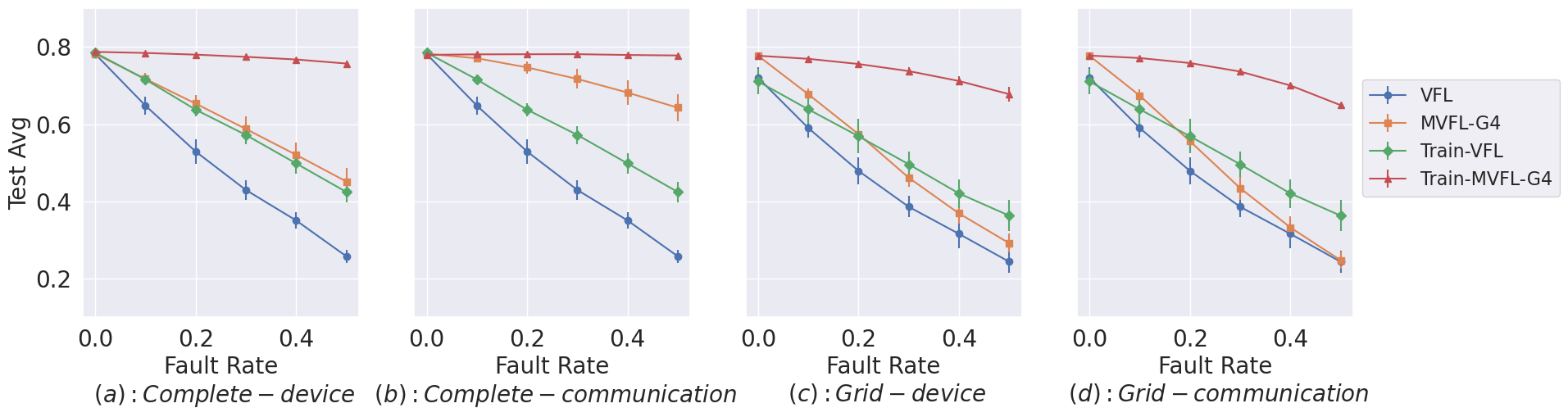
Figure 4: Test average accuracy with and without train faults for StarCraftMNIST with 16 devices. Here we include models trained under fault rate 30% (marked by ’Train-’). All results are averaged over 16 runs and error bar represents standard deviation. Across different configurations, MVFL-G4 has the highest average performance, while VFL performance is not robust as fault rate increases. Irrespective of the model, training with faults makes the model robust against test time faults

Table 1: Best models for 2 complete-communication fault rates within 1 standard deviation are bolded (we do not bold best models for worst metric because all models achieve 0 accuracy. More detailed results with standard deviation are shown in the appendix.

		MNIST				SCMNIST				CIFAR10
		Avg	Rand	Best	Worst	Avg	Rand	Best	Worst	Avg	Rand	Best	Worst
Fault Rate = 0.3	VFL	0.507	nan	nan	nan	0.430	nan	nan	nan	0.267	nan	nan	nan
2-14	MVFL	0.705	0.524	0.997	0.000	0.592	0.444	0.970	0.000	0.342	0.269	0.906	0.000
	MVFL-G4	0.897	0.655	0.938	0.006	0.717	0.533	0.827	0.004	0.354	0.277	0.606	0.002
	DMVFL	0.709	0.525	0.965	0.001	0.573	0.433	0.920	0.001	0.287	0.231	0.761	0.000
	DMVFL-G4	0.799	0.591	0.875	0.005	0.646	0.482	0.783	0.005	0.322	0.255	0.584	0.002
Fault Rate = 0.5	VFL	0.294	nan	nan	nan	0.258	nan	nan	nan	0.181	nan	nan	nan
2-14	MVFL	0.518	0.311	0.987	0.000	0.465	0.280	0.969	0.000	0.264	0.182	0.901	0.000
	MVFL-G4	0.732	0.415	0.887	0.000	0.643	0.372	0.846	0.000	0.267	0.182	0.684	0.000
	DMVFL	0.429	0.266	0.915	0.000	0.368	0.233	0.891	0.000	0.186	0.143	0.773	0.000
	DMVFL-G4	0.547	0.324	0.800	0.000	0.475	0.284	0.773	0.000	0.213	0.156	0.656	0.000

Different Test Fault Rates and Patterns

As shown in Figure 3, under no training faults, we investigate how different models perform under (1) different test fault rates (2) different fault type i.e., device or communication (3) different network i.e., complete network or grid network. In Figure 3, we first note that when there is no train fault rate, as the test fault rate becomes higher, the performance of all models always become worse as we expect. First focusing on the complete baseline network (Figure 3 (a) and (b)), it can be seen that both MVFL and DMVFL outperform VFL, which demonstrates the benefit of replicating servers. It seems that extra communication round between servers does not help in most cases which could result from the fact that we need to keep the total number of parameters the same, but DMVFL requires more communication and could receive more faulted information. In the case of complete-communication, when fault rate is low, DMVFL outperforms MVFL and we think this shows a tradeoff between benefiting from extra communication and receiving more faulted representation while the capability of the model is roughly the same. Regarding gossiping, it helps both MVFL and DMVFL mainly in the case of communication fault. We believe this is because in the device fault case, irrespective of number of gossip rounds, the representations from faulted device cannot be obtained. On the other hand, multiple gossip rounds in communication fault scenario has the effect of balancing out the lost representation at a client via neighboring connections. Switching to the grid baseline network, a major observation here is the degradation in the performance of both DMVFL and DMVFL-G4. We conjecture that in this case, clients can only directly communicate with neighboring clients, thus it’s harder to get information from clients far away and extra communication leads to less benefit while the smaller network size and receiving more faulted representation become a bottleneck. Similarly, we notice that MVFL outperforms MVFL-G4 when fault rate is very high, as there is a much higher chance that the network is disconnected in comparison to complete baseline network. In short, we conclude that when trained with no faults, MVFL is overall the best model while gossiping helps except with high fault rates under the grid baseline network.

Train Faults

We further explore the effect of training with faults on the average performance of models for different test time faults. Figure 4 shows that training with faults improves the average performance during test time faults. We conjecture that faults during training helps with regularizing the model, similar to the effect dropout has. Even when training with faults, MVFL and it’s gossip variant outperforms VFL. Further investigation with training faults is covered in the Appendix.

Ablation Studies

We study the effect of depth for DMVFL and gossip rounds on average performance. It was based on this study that we selected the configurations of models that are presented in Figure 3 and Figure 4. Due to space constraints, the results are presented in the Appendix.

Other metrics

In Table 1 performance of all the models across the four metrics are presented for 3 datasets and 2 complete-communication fault rates. Across the different datasets, when comparing average performance, MVFL or it’s gossip variant are more robust than VFL. Also, it is not surprising that the trends observed for Avg and Rand metric are similar. Furthermore, comparing MVFL-G with MVFL, it is seen that while the average performance is higher for the gossip variant, it is accompanied by a lower Best performance.

In Section 4.2 we highlight results, Test (Inference) Faults [Summarized in Figure 3] and Train Faults [Summarized in Figure 4]) that use the proposed methods. Furthermore, in depth analysis using train and test time faults for these methods are explored in the Appendix. The symmetry of the toy example (without any dynamic conditions) in Figure 2 hides the complexity.

In more complex cases with non-symmetric topologies (example shown in Appendix), each layer might learn something different beyond mere randomness. We agree that Deep MVFL may not provide additional benefits in our current scenario and is a negative result.

Ultimately, we expect new architectures or training algorithms may be needed to enable better IL algorithms.

5 Conclusion

In this paper, we carefully defined Internet Learning, proposed several IL methods based on VFL, developed an IL testbed, and evaluated and compared IL performance across various fault models and datasets. While this work provides the foundation for IL, it opens many new directions such as heterogeneous devices or models, new architectures, or new fault models. Furthermore, a real IL system may need to operate in an online streaming manner, handle asynchronous communication, adapt to smoothly changing network topologies, or minimize latency, communication cost, or power. Ultimately, we believe this paper provides the first step towards highly fault-tolerant learning on dynamic networks.

Appendix

Appendix John Doe

In the main paper, the following information were listed to be provided in the Appendix section and they can be found in the Appendix per the listing below:

1. Relation to GNN from Section 2.3 can be found in Section B

2. Analysis for different number of devices/clients from Section 4.1 can be found in Section D.5

3. Specifics on model architecture from Section 4.1 can be found in Section C.3

4. Further analysis on gossiping methods from Section 4.1 can be found in Section D.1

5. Grid graph construction details from Section 4.1 can be found in Section C.2

6. Further study with training faults from Section 4.2 can be found in Section D.2

7. Ablation studies from Section 4.2 can be found in Section D.3

8. Further details on metrics from Table 1 can be found in Section D.4

Appendix A Device and Communication Fault Visualization

We show in Figure 5 the visual representation of communication and device fault under the MVFL method. Although, we present the scenario for only one method, by extension the visualization is similar for VFL, DMVFL and the gossip variants.

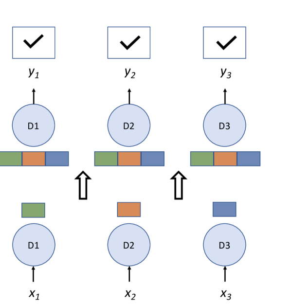
(a) MVFL

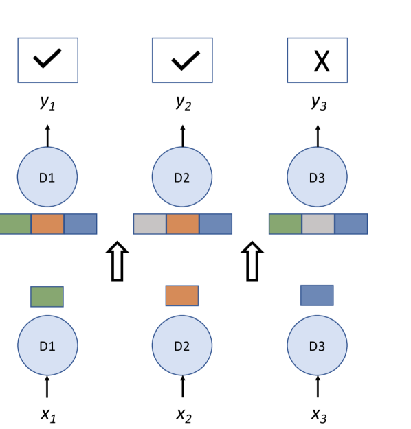
(b) MVFL-Communication Fault

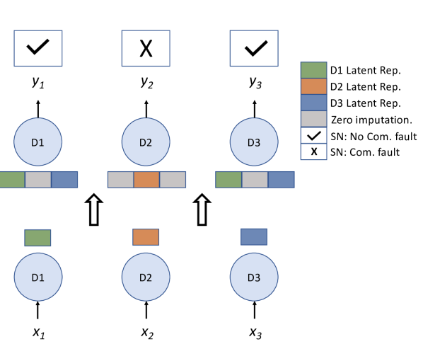
(c) MVFL-Device Fault

Figure 5: Illustration of communication and device faults for a 3 device network for the MVFL method. (a) Fully connected MVFL setup. The check mark indicates that there is no fault in the final communication between device and special node (SN) as defined in Section 2.3 of the main paper (b) Representation with communication faults. In this example communication from D1 to D2 and D2 to D3 is faulted. To account for the missing values, we do zero imputation. $X$ indicates that the communication between D3 and SN is faulted. Hence, the output at SN will be a class selected with uniform probability among all the classes (c) In device faults, the faulted device do not communicate with any other devices and missing values are accounted for by zero imputation. In this example, D2 is assumed to be faulted, hence the information from D2 is not passed to D1 or D3 and it does not produce an output. The output at SN for $D_{2}$ will be a class selected with uniform probability among all the classes

Appendix B Further Discussion and Limitations

Distributed Inference Algorithm’s Resemblance to GNNs:

The form of our distributed inference algorithm in the main paper has a superficial resemblance of the computation of graph neural networks (GNN) [23] but with important semantic and syntactic differences. Semantically, unlike GNN applications whose goal is to predict global, node, or edge properties based on the graph edges, our goal is to do prediction well given any arbitrary edge structure. Indeed, the edges in our dynamic network are assumed to be independent of the input and task—rather they are simply constraints based on the network context of the system. Syntactically, our inference algorithm differs from mainstream convolutional GNNs because convolutional GNNs share the parameters across clients (i.e., $\theta_{c}^{(t)}=\theta^{(t)}$) whereas in our algorithm the parameters at each client are not shared across clients (i.e., $\theta_{c}^{(t)}\neq\theta_{c^{\prime}}^{(t)}$). Additionally, most GNNs assume the aggregation function $g$ is permutation equivariant such as a sum, product or maximum function. However, we assume $g$ could be any aggregation function. Finally, this definition incorporates the last processing function $h$ that represents the final communication round to an external entity (Main Paper Section 2.3).

Design for extreme conditions:

The proposal to consider extreme conditions as the basis for Internet Learning (IL), is inspired by impressive performance of technologies such as the internet and autonomous vehicles, that have been developed to handle rare or catastrophic events. To elaborate, the foundation of the Internet is the development of packet switching to replace circuit switching for communication [1, 7]. Indeed, Baran, [1] motivated packet switching almost entirely by the concept of survivability or reliability of the communication network under near catastrophic and adversarial faults (e.g., a nuclear bomb or enemy raid). For autonomous cars, the learning-based systems need to handle all circumstances well particularly rare circumstances where a mistake could cause a human fatality (e.g., driving in a snowstorm with limited visibility in a construction site). Thus, designing for the worst case is critical in this application as well. Like circuit switching, current ML algorithms (particularly standard end-to-end backpropagation) require careful synchronization and would likely degrade significantly under benign failures. Yet, highly fault-tolerant learning algorithms could have wide applicability.

Alternative Approaches:

Although in the main paper we presented novel methods, we believe that methods which allow for asynchronicity and decoupling of forward and backward passes during training/inference will be critical to the development of future methods. To that end, localized learning algorithms, such as Hinton, [13], Høier et al., [14], Detorakis et al., [8], Movellan, [21], Czarnecki et al., [6], Belilovsky et al., [2, 3], may play an important role in the development of IL methods that have the desired robustness properties for the IL context.

Limitations:

In recent times, a key consideration for distributed learning paradigms, such as Federated Learning, has been to ensure that clients or devices data remains private. Given the distributed nature and the ability of the devices/clients in IL to interact with each other, we believe that, though not the primary property of an IL system, privacy and security of an IL system is an important direction for future work. Furthermore, the experiments in the main paper were simulated with no communication latency. However, it is a salient practical consideration. Therefore, in the future it will be crucial to consider this in the IL paradigm and develop methods that can accommodate for asynchronous or semi-synchronous updates. Finally, we also note that we assumed the communication graph was constant for the entire forward and backward operations. This is unlikely to hold in practice but may change every communication round. Further implementation effort would be required to implement dropping on both the forward and backward passes of training.

Appendix C Experiment Details

C.1 Datasets

For the experiments presented in this paper, following are the datasets that were used:

StarCraftMNIST(SCMNIST): Contains a total of 70,000 28x28 grayscale images in 10 classes. The data set has 60,000 training and 10,000 testing images. For experiments, all the testing images were used, 48,000 training images were used for training and 12,000 training images were used for validation study.

MNIST: Contains a total of 70,000 28x28 grayscale images in 10 classes. The data set has 60,000 training and 10,000 testing images. For experiments, all the testing images were used, 48,000 training images were used for training and 12,000 training images were used for validation study.

CIFAR-10: Contains a total of 60,000 32x32 color images in 10 classes, with each class having 6000 images. The data set has 50,000 training and 10,000 testing images. For experiments, all the testing images were used, 40,000 training images were used for training and 10,000 training images were used for validation study.

C.2 Graph construction

In the main paper as well as in the Appendix the terms client and devices are used interchangeably. In Section 4.1 of the main paper, two different graphs were introduced: Complete and Grid. To elaborate how these graphs are constructed for a set of 16 clients, we take an example of an image from each of the three datasets and split it up into 16 sections, as illustrated in Figure 6.

For a Complete graph, all the devices are connected to the server. For instance, if $D_{1}$ is selected as the server, then all the other devices $D_{i}$ for $i$ = $2$, $3$, …, $16$ are connected to $D_{1}$. To construct Grid graph, we use compute a Distance parameter. For Grid graph, distance returns true if a selected device lies horizontally or vertically adjacent to a server and only under this circumstance it is connected to the server otherwise it is not. For example, in Figure 6, if $D_{3}$ is selected as the server, then $D_{2}$, $D_{4}$ and $D_{7}$ are the only devices connected to $D_{3}$. Another example will be, if $D_{13}$ is selected as the server, then $D_{9}$ and $D_{14}$ are the only ones connected to the server.

Irrespective of the base graph, Grid or Complete, when training or testing faults are applied to the selected base graph, during implementation it is assumed that the graph with incorporated faults stays constant for one entire batch and then the graph is reevaluated for the next batch. In our experiments, the batch-size is taken to be 64.

Furthermore, in Figure 7 we highlight a few examples, to illustrate with MNIST images, why in some cases it is easy to distinguish between images based on partial information and while in other situations, it is not. Thus, device connectivity plays a crucial role in enabling classification tasks.

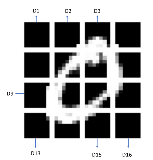
(a) MNIST

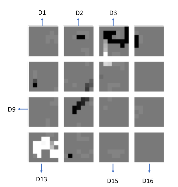
(b) StarCraftMNIST(SCMNIST)

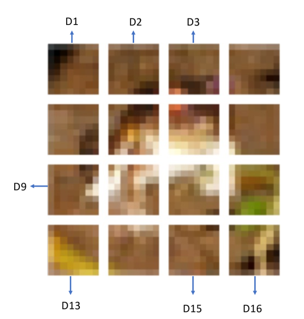
(c) CIFAR-10

Figure 6: (a)MNIST, (b)SCMNIST, (c)CIFAR-10 Image split into 16 sections. Each section is assigned to a device/client.$D_{i}$ denotes a device/client

(a) 1

(b) 9

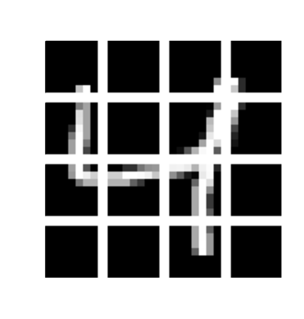
(c) 4

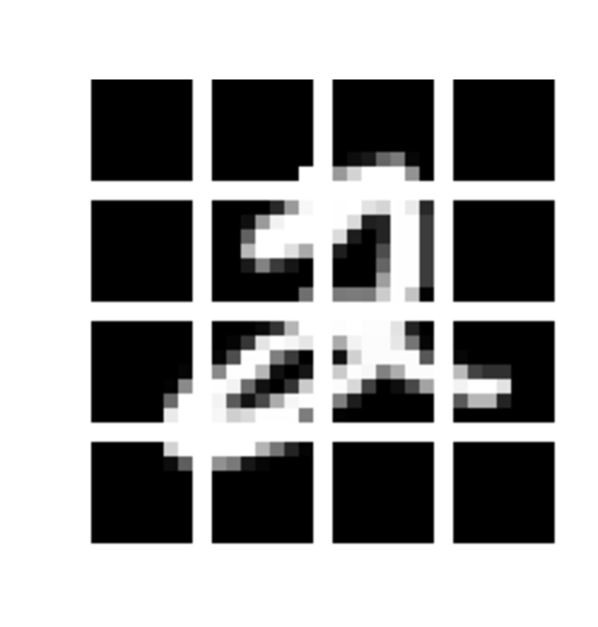
(d) 2

Figure 7: Based on limited information, some images are easy to distinguish from one another, others are not. For instance, based on the information from just bottom half of the devices, it is hard to distinguish between (a) and (b) while differentiating between images (c) and (d) is achievable just based in the bottom half of devices.

C.3 Training

For all of our experiments, we train the model for 100 epochs and we always report the result using the model checkpoint with lowest validation loss. We use a batch size of 64 and Adam optimizer with learning rate 0.001 and $(\beta_{1},\beta_{2})=(0.9,0.999)$. All experiments are repeated using seed 1,2,…,16.

For 16 devices with all datasets, each device in VFL and MVFL has a model with the following structure: Linear(49,16),ReLU,Linear(16,4),ReLU,MP,Linear(64,64),ReLU,Linear(64,10) where MP means message passing. For 4 devices with all datasets, each device in VFL and MVFL has a model with the following structure: Linear(196,64),ReLU,Linear(64,16),ReLU,MP,Linear(64,64),ReLU,Linear(64,10). For 49 devices with all datasets, each device in VFL and MVFL has a model with the following structure: Linear(16,4),ReLU,Linear(4,2),ReLU,MP,Linear(98,98),ReLU,Linear(98,10).

For 16 devices with all datasets, each device in DMVFL has a model with the following structure: Linear(49,16),ReLU,Linear(16,4),ReLU,MP,DeepLayer,Linear(64,10). For 4 devices with all datasets, each device in DMVFL has a model with the following structure: Linear(196,64),ReLU,Linear(16,4),ReLU,MP,DeepLayer,Linear(64,10). For 49 devices with all datasets, each device in DMVFL has a model with the following structure: Linear(16,4),ReLU,Linear(16,4),ReLU,MP,DeepLayer,Linear(98,10). DeepLayer are composed of a sequence of MultiLinear(64,16) based on depth and MultiLinear(x)=Mean(ReLU(Linear(64,16)(x)),…,ReLU(Linear(64,16)(x))). Here we use multiple perceptrons at each layer to make sure the number of parameters between MVFL and DMVFL. For example, for 16 devices and a depth of 2, we use $16/2=8$ perceptrons at each layer.

All experiments are performed on a NVIDIA RTX A5000 GPU.

Appendix D Additional Experiments

D.1 Gossip Methods

Here we compare 4 different methods of gossip. Let $y^{(0)}_{c,i}$ be the logit at client $c$ for class $j$ (input to the gossip layer) and $N_{g}$ indicate the number of gossiping (averaging). We want to investigate the effect of log probability normalization via log softmax throughout the gossiping strategy. We propose several different methods that add logsoftmax normalization in multiple places during gossip. Below we formalize the computation of each gossip methods and the final output would be used for computing negative loglikelihood loss.

(1) Logit: We take the average of raw output of the final layer of network and apply LogSoftmax at the end of gossipping.

$$y^{(1)}_{c,j} =y^{(0)}_{c,j}$$

$$y^{(n+1)}_{c,j} =\frac{1}{C}\sum_{c^{\prime}}y^{(n)}_{c^{\prime},j}\quad\forall n\in\{1,\dots,N_{g}\}$$

$$y^{(final)}_{c,j} =\left[\operatorname{LogSoftmax}(y^{(N_{g}+1)}_{c,1},\dots,y^{(N_{g}+1)}_{c,m})\right]_{j}$$

(2) Gm (geometric mean): We apply LogSoftmax to the final output of the network to get proper log probabilities for each head. Then we run gossipping, and we also normalize the log probabilities after each gossip round to make sure that they always represent log probabilities in each gossip round.

$$y^{(1)}_{c,j} =\left[\operatorname{LogSoftmax}(y^{(0)}_{c,1},\dots,y^{(0)}_{c,m})\right]_{j}$$

$$y^{(n+1)}_{c,j} =\frac{1}{C}\sum_{c^{\prime}}y^{(n)}_{c^{\prime},j}-\left[\operatorname{LogSumExp}(\frac{1}{C}\sum_{c^{\prime}}y^{(n)}_{c^{\prime},1},\dots,\frac{1}{C}\sum_{c^{\prime}}y^{(n)}_{c^{\prime},m})\right]_{j}\quad\forall n\in\{1,\dots,N_{g}\}$$

$$y^{(final)}_{c,j} =y^{(N_{g}+1)}_{c,j}$$

(3) Ugm (unnormalized geometric mean): we apply LogSoftmax to the final output of the network. Then we run gossipping without normalizing the output after each round. Notice that this does not renormalize at each round like in Gm.

$$y^{(1)}_{c,j} =\left[\operatorname{LogSoftmax}(y^{(0)}_{c,1},\dots,y^{(0)}_{c,m})\right]_{j}$$

$$y^{(n+1)}_{c,j} =\frac{1}{C}\sum_{c^{\prime}}y^{(n)}_{c^{\prime},j}\quad\forall n\in\{1,\dots,N_{g}\}$$

$$y^{(final)}_{c,j} =y^{(N_{g}+1)}_{c,j}$$

(4) Ugmn (unnormalized geoemetric mean and normalizing): This is the same as ugm except that we normalize the output after the final round of gossip such that we are using proper log probabilities when computing negative log likelihood loss.

$$y^{(1)}_{c,j} =\left[\operatorname{LogSoftmax}(y^{(0)}_{c,1},\dots,y^{(0)}_{c,m})\right]_{j}$$

$$y^{(n+1)}_{c,j} =\frac{1}{C}\sum_{c^{\prime}}y^{(n)}_{c^{\prime},j}\quad\forall n\in\{1,\dots,N_{g}\}$$

$$y^{(final)}_{c,j} =y^{(N_{g}+1)}_{c,j}-\left[\operatorname{LogSumExp}(\frac{1}{C}\sum_{c^{\prime}}y^{(N_{g}+1)}_{c^{\prime},1},\dots,\frac{1}{C}\sum_{c^{\prime}}y^{(N_{g}+1)}_{c^{\prime},m})\right]_{j}$$

In Figure 8, we show the results of these models with no training faults but with various levels of test faults. We notice that, in most cases, ugm outperforms all others while the remaining three methods have similar performance. Thus, surprisingly, because all other methods normalize the values at the end, it seems that the most important difference (and significantly important) is whether logsoftmax is used at the end immediately prior to being passed to the cross entropy loss. Other intermediate normalizations before or during gossiping (as in logits, gm) do not seem to have a significant affect on the performance but normalization at the end as in ugmn does change the performance. This result is surprising because this means that the values being passed to the cross entropy loss are unnormalized log probabilities rather than proper log probabilities.

We conjecture this surprising phenomena is caused by the idea that with normalization a very confident prediction from one classifier head can dominate the gossip-based prediction. Specifically, the training loss can be reduced by focusing on a single classifier head’s prediction and making it very confident while ignoring other classifier heads’ predictions. While this works during training because there are no faults, at test time, the well-trained classifier head may fault leaving only poorly trained classifier heads. On the other hand, without normalization, each classifier head more evenly contributes to the final gossip-based prediction and thus all classifier heads have to predict reasonably well. When the task gets more difficult (e.g., fault rate gets higher or the baseline network becomes grid), it would be harder for some devices (especially those with less meaningful data on their own) to make correct predictions and ugm would be better at optimizing those devices. This also aligns with our observation that the gap gets minimum when there is no fault. Even though this is a uncommon technique to use, we think it’s an interesting observation and report it here. And as gm is a more standard technique in the literature, we use it for all other experiments in this paper and leave further investigation of gossip methods as future works.

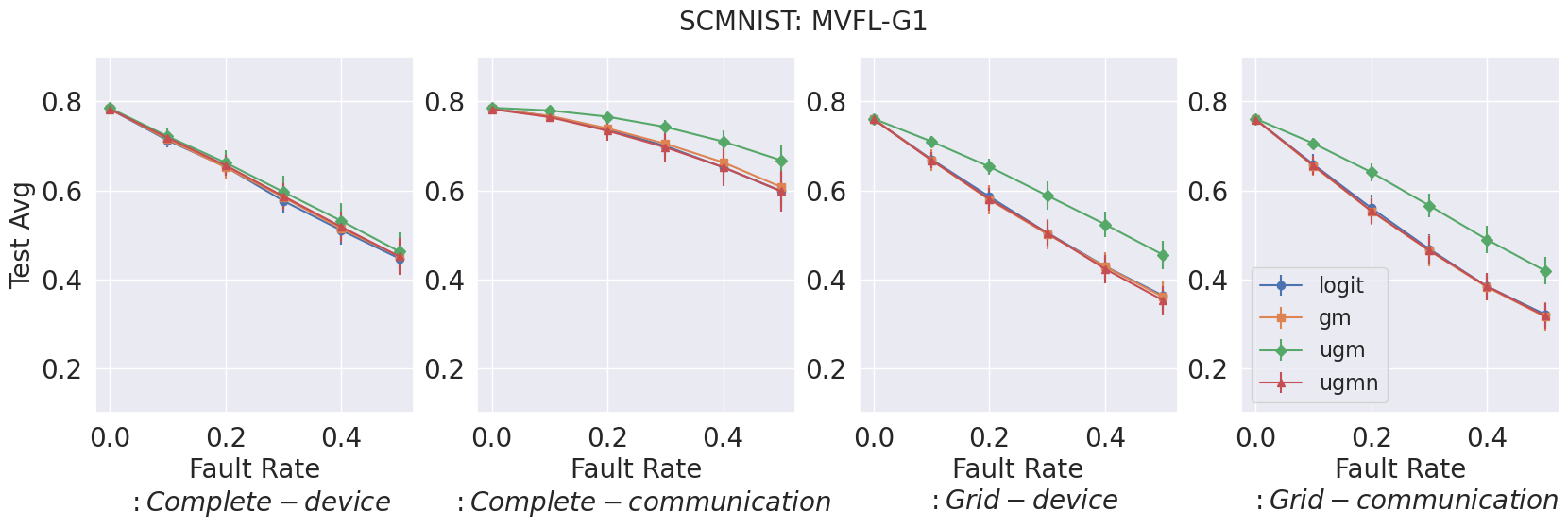
(a) MVFL-G1

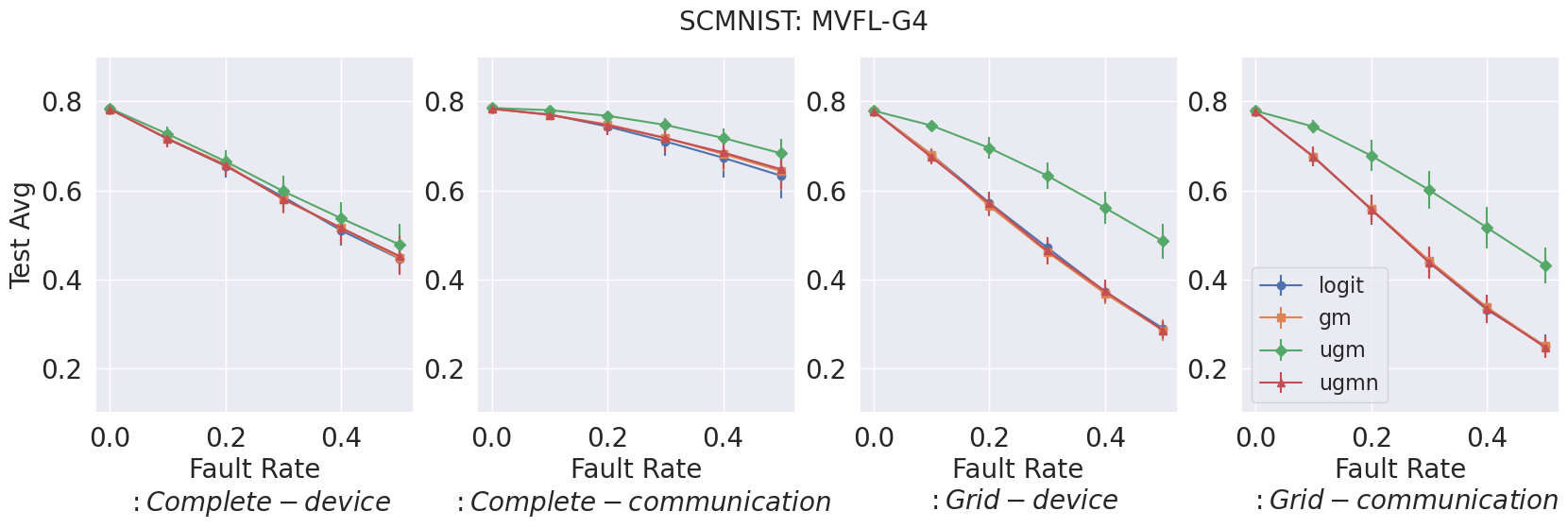
(b) MVFL-G4

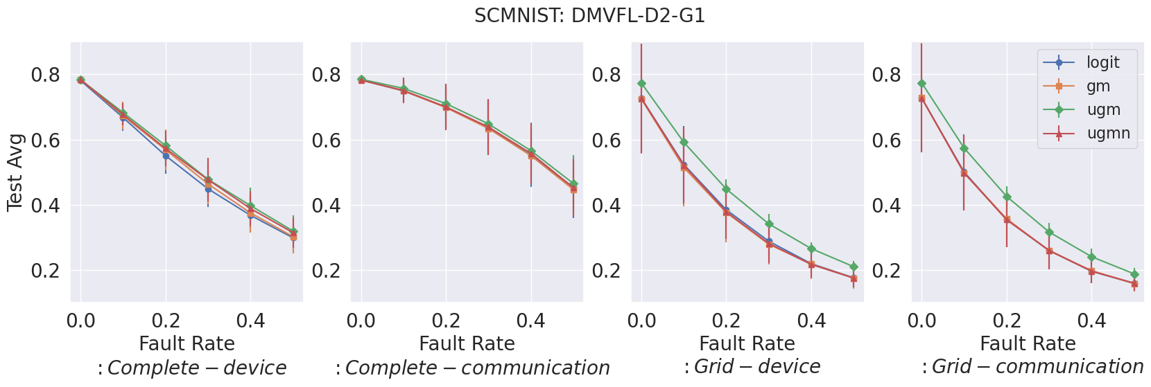
(c) DMVFL-D2-G1

(d) DMVFL-D2-G4

Figure 8: Comparison of gossip methods with different models for SCMNIST.

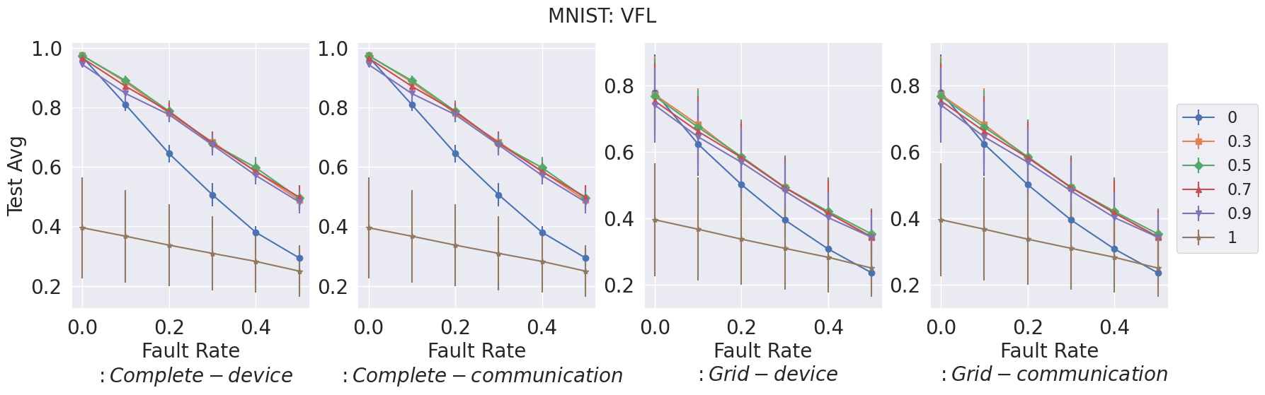
(a) VFL

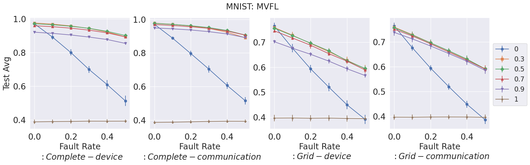
(b) MVFL

(c) MVFL-G4

Figure 9: Test average accuracy with different communication training fault rates for MNIST with 16 devices. Across different configurations,training with faults makes the model robust against test time faults

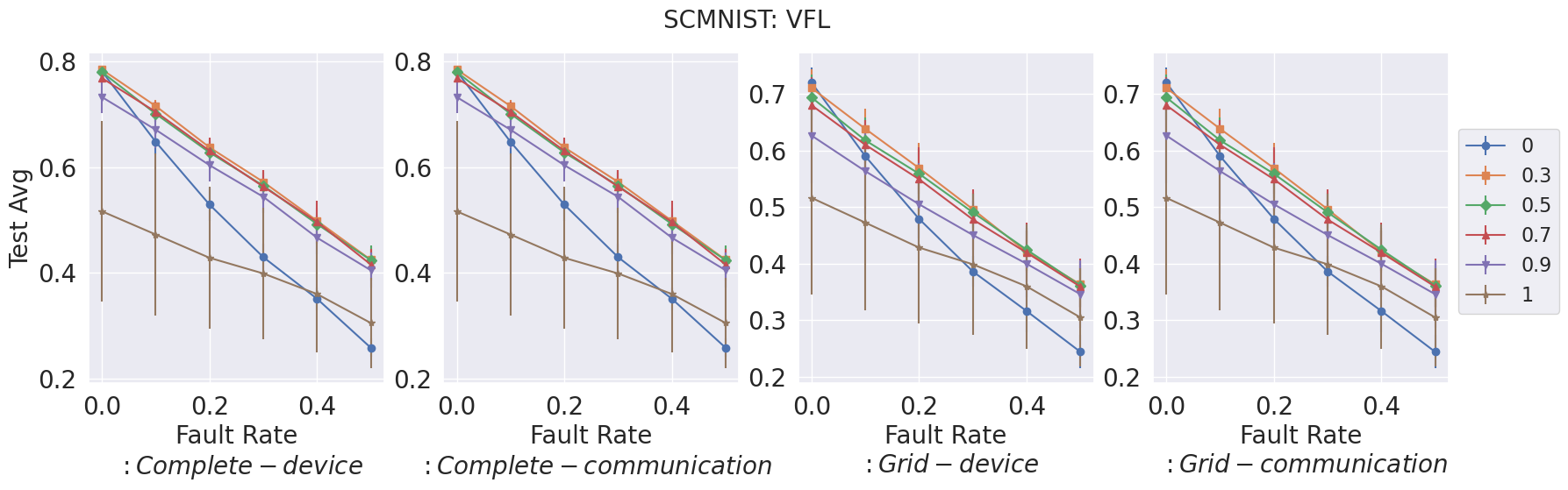
(a) VFL

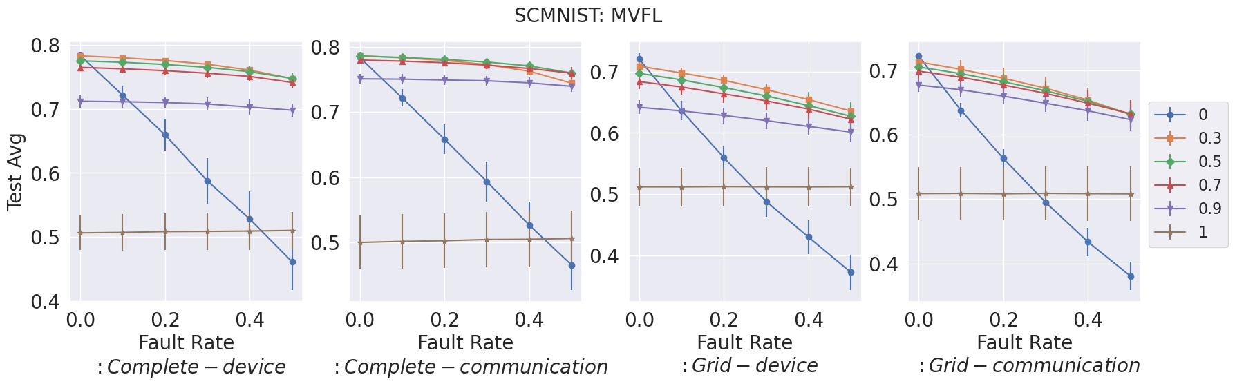
(b) MVFL

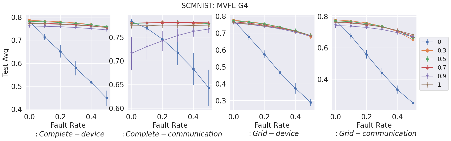
(c) MVFL-G4

Figure 10: Test average accuracy with different communication training fault rates for SCMNIST with 16 devices. Across different configurations,training with faults makes the model robust against test time faults

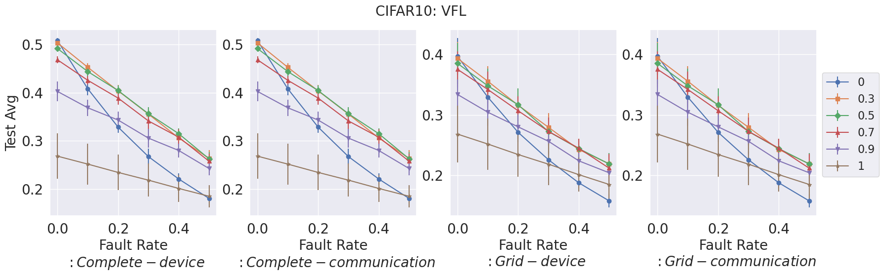
(a) VFL

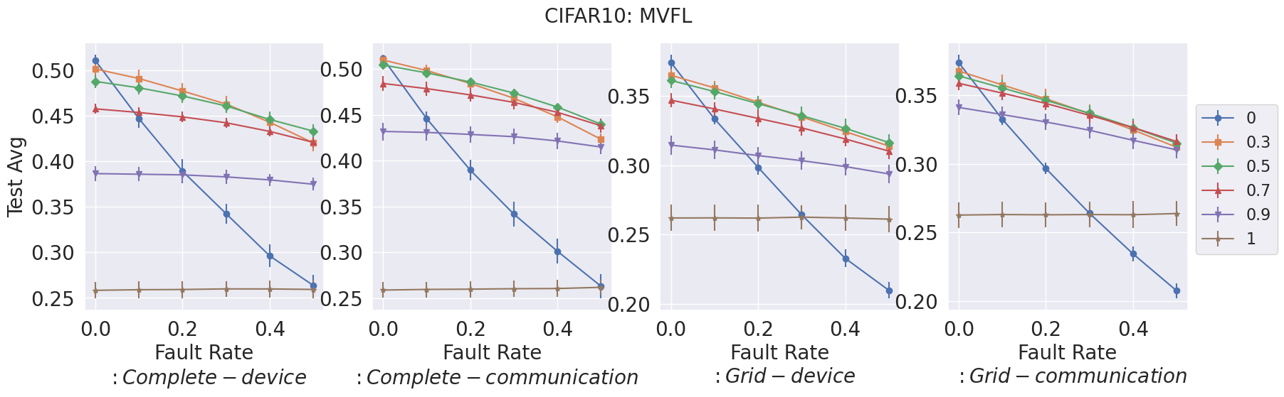
(b) MVFL

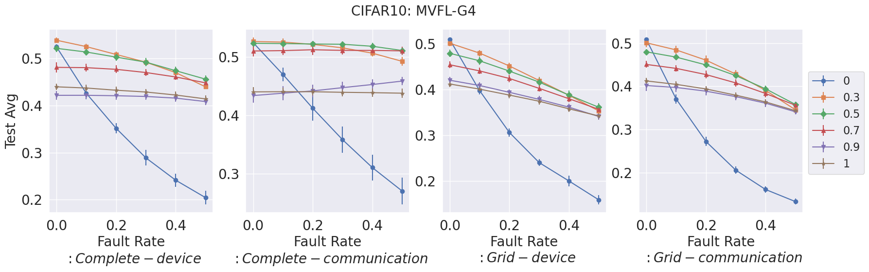
(c) MVFL-G4

Figure 11: Test average accuracy with different communication training fault rates for CIFAR10 with 16 devices. Across different configurations,training with faults makes the model robust against test time faults

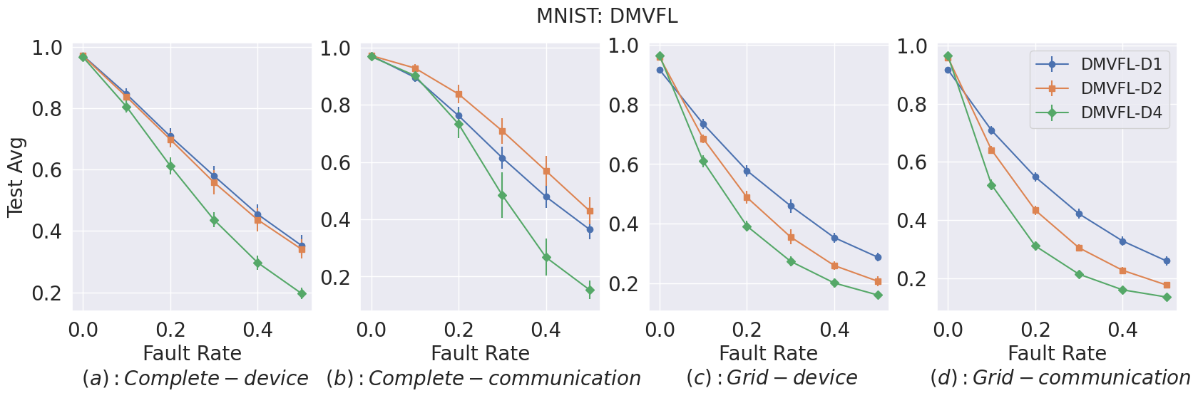
Figure 12: Average performance as a function of Depth of DMVFL for MNIST.

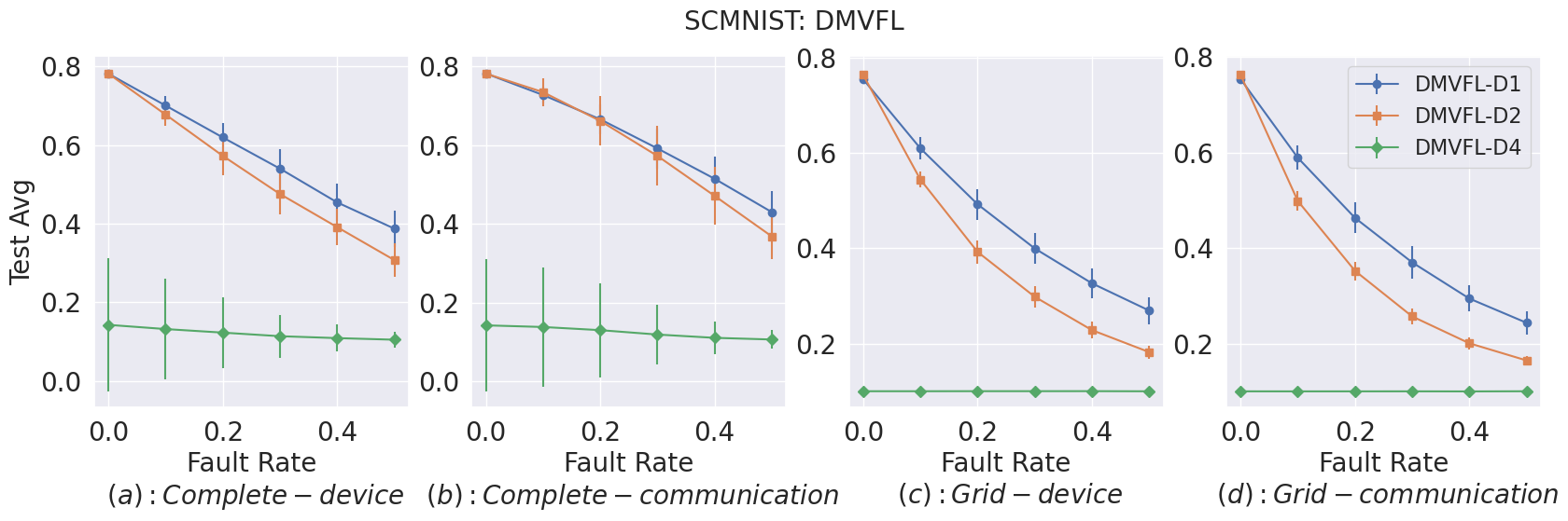
Figure 13: Average performance as a function of Depth of DMVFL for SCMNIST.

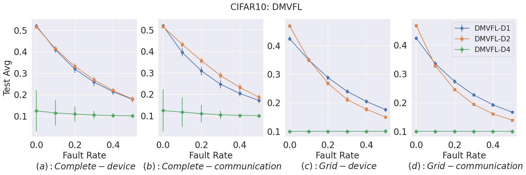
Figure 14: Average performance as a function of Depth of DMVFL for CIFAR-10.

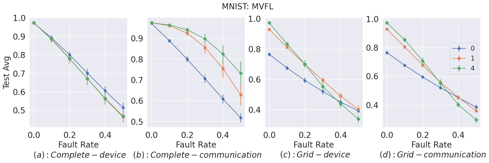
(a) MNIST

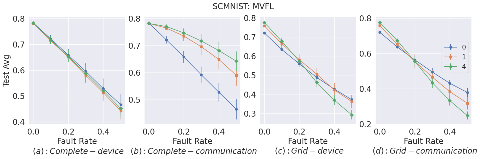
(b) SCMNIST

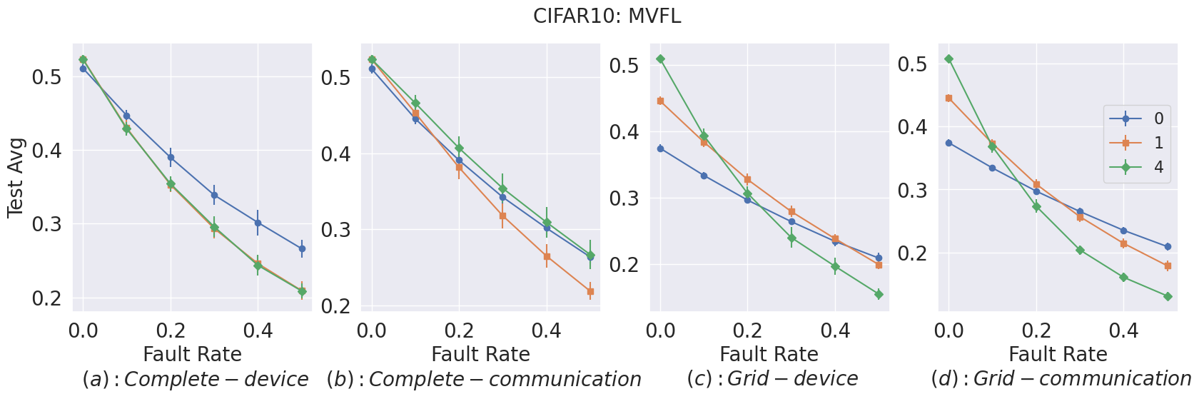
(c) CIFAR-10

Figure 15: MVFL: Effect of different rounds of Gossip on average performance when evaluated with no training faults but only test time faults for 16 devices

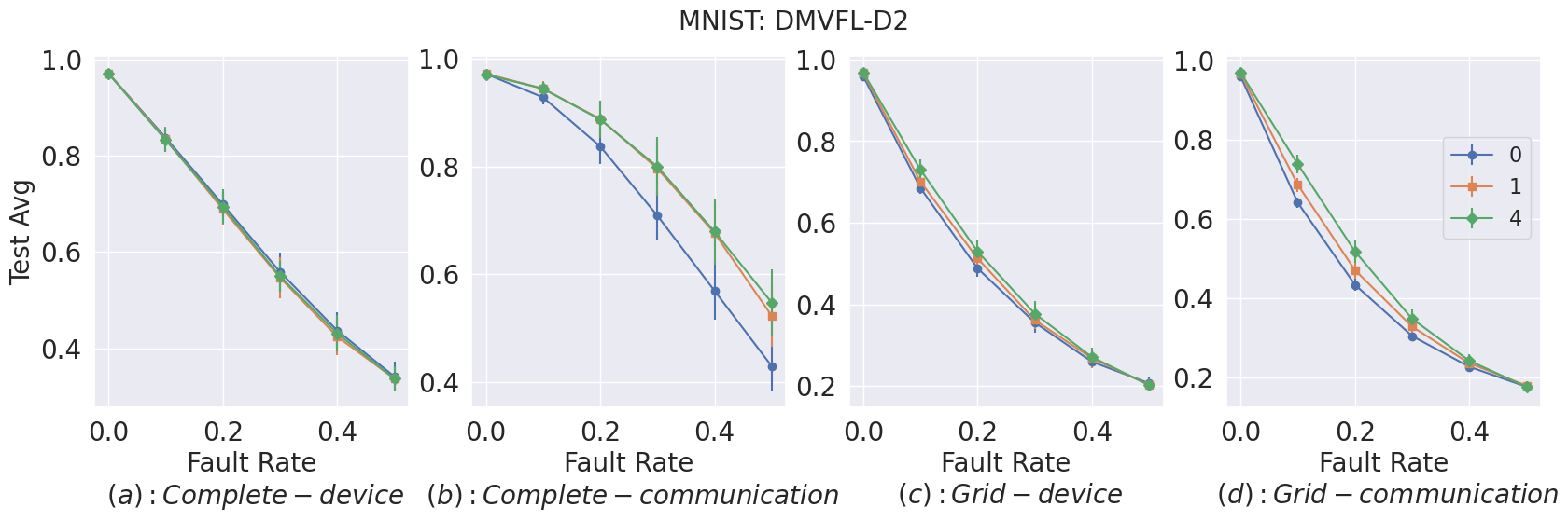
(a) MNIST

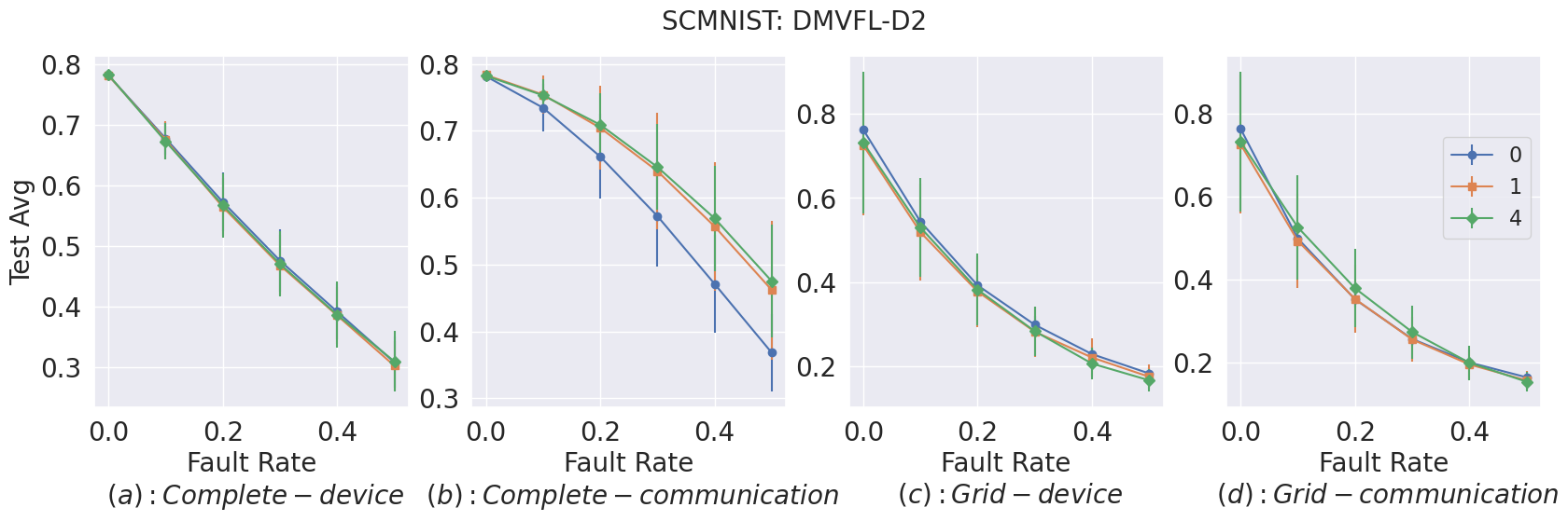
(b) SCMNIST

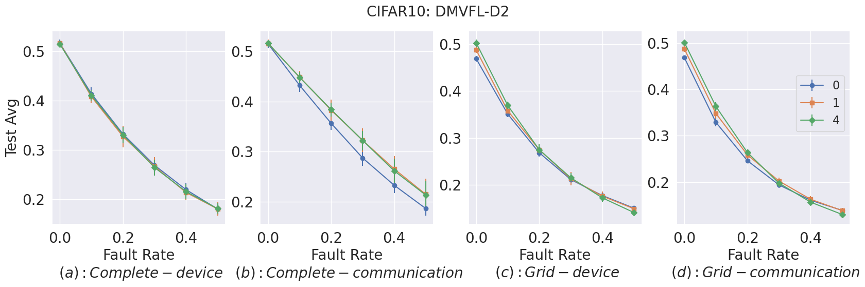
(c) CIFAR-10

Figure 16: DMVFL-D2: Effect of different rounds of Gossip on average performance when evaluated with no training faults but only test time faults for 16 devices

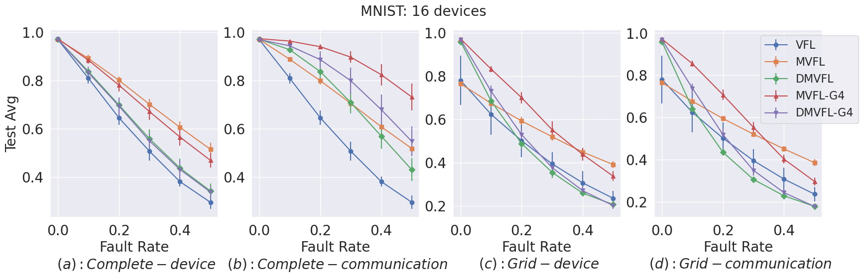
(a) Avg

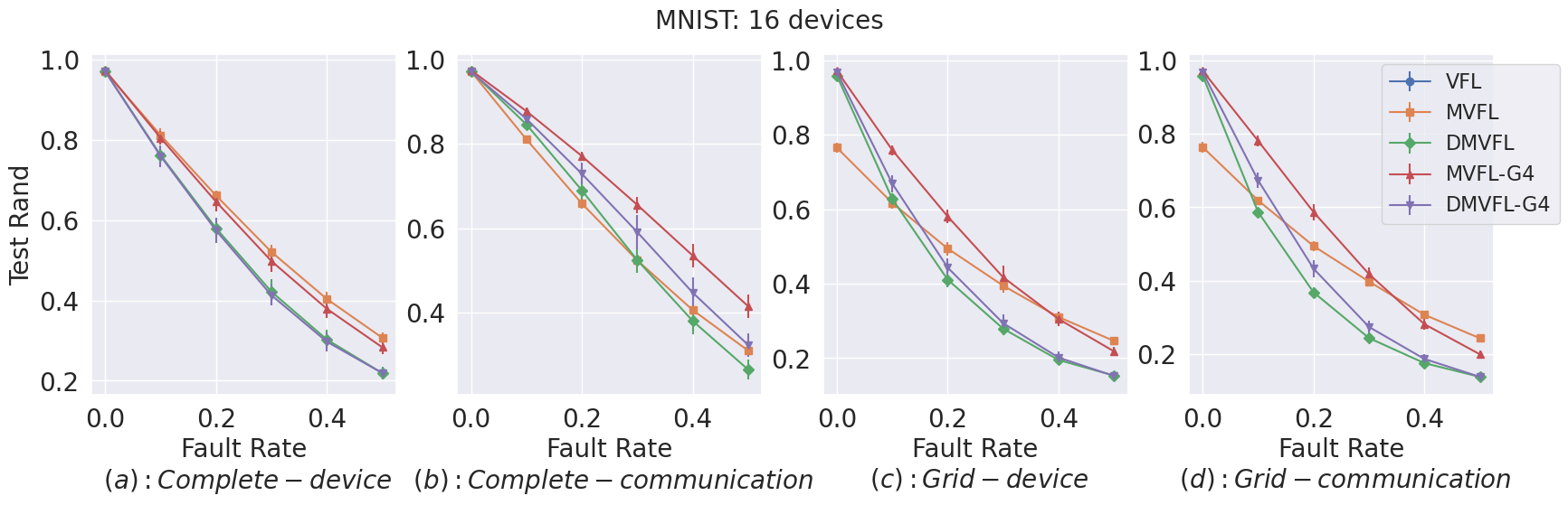
(b) Rand

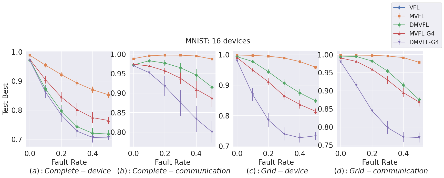
(c) Best

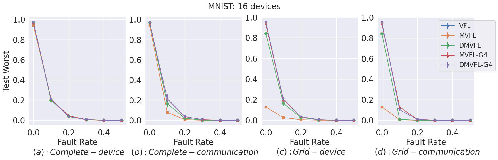
(d) Worst

Figure 17: All metrics reported for MNIST with 16 devices and only test time faults

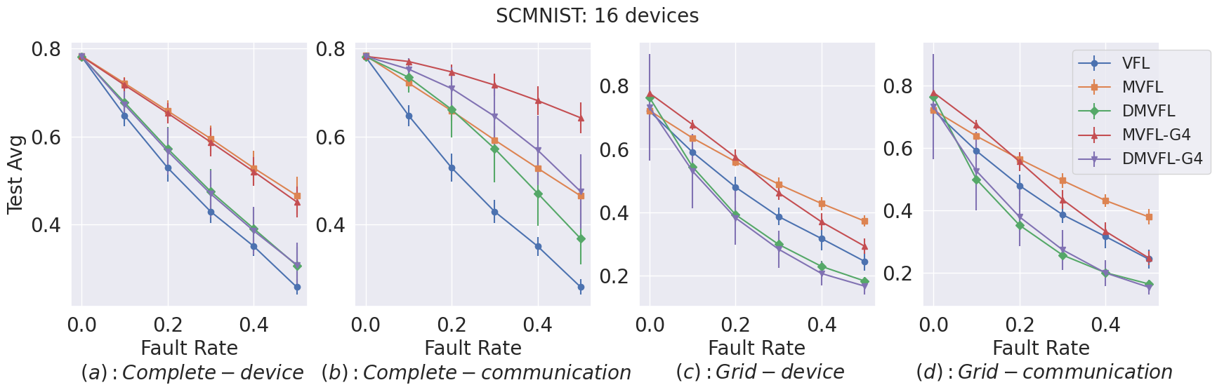
(a) Avg

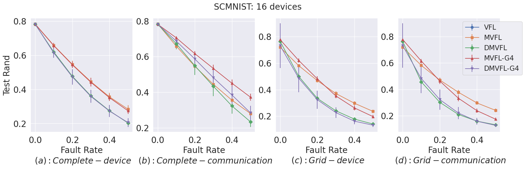
(b) Rand

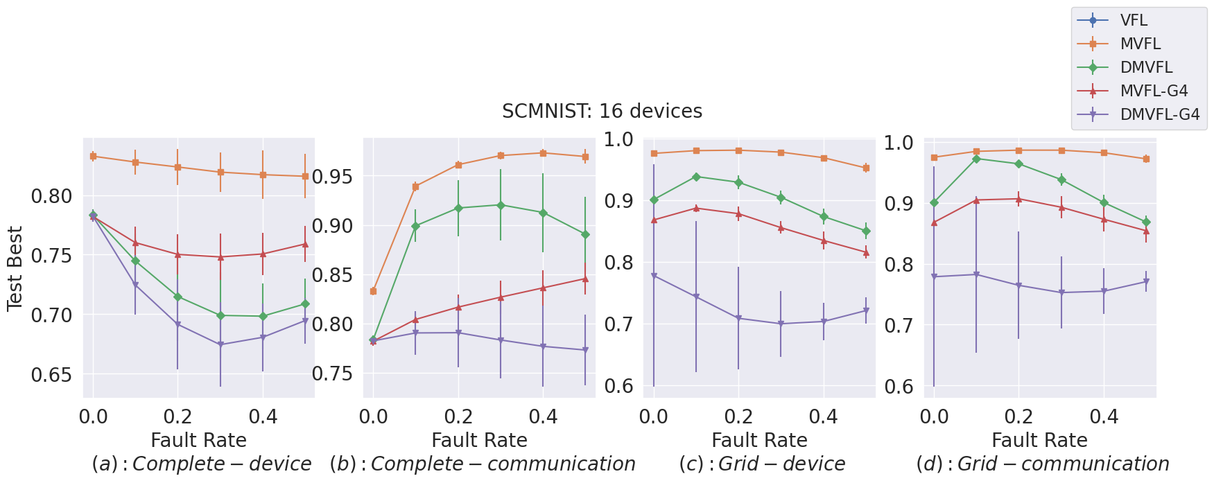
(c) Best

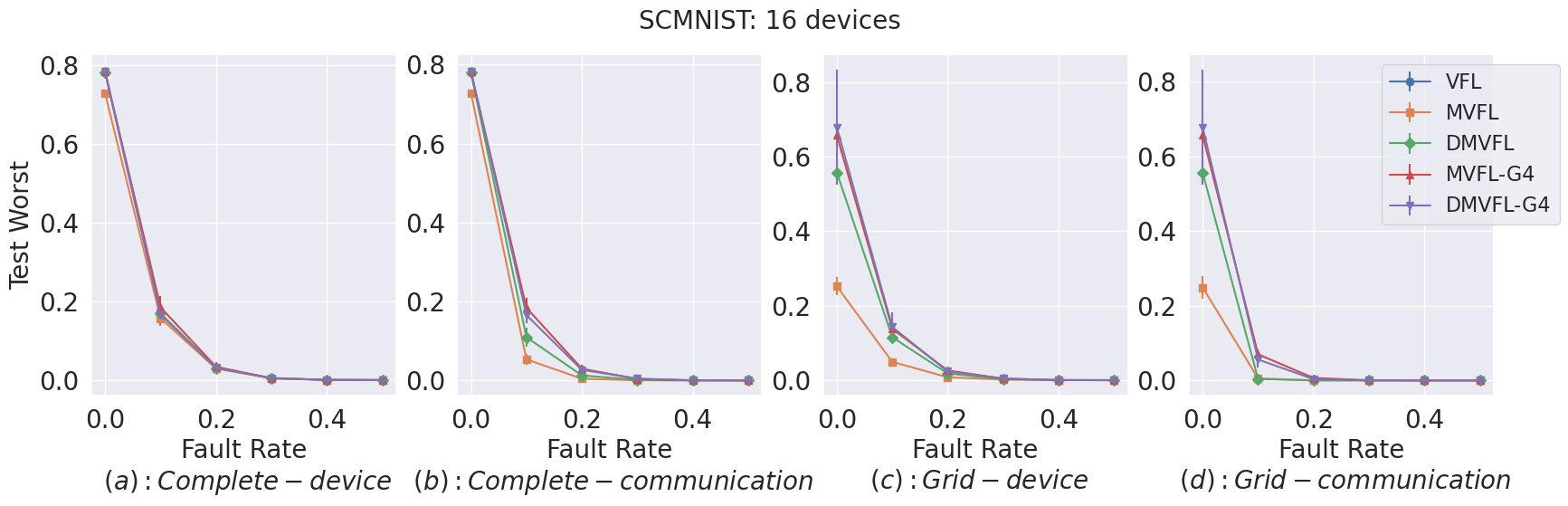
(d) Worst

Figure 18: All metrics reported for SCMNIST with 16 devices and only test time faults

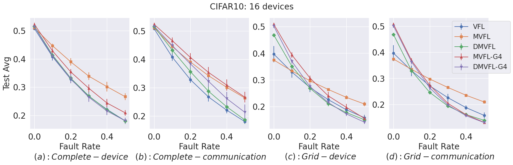
(a) Avg

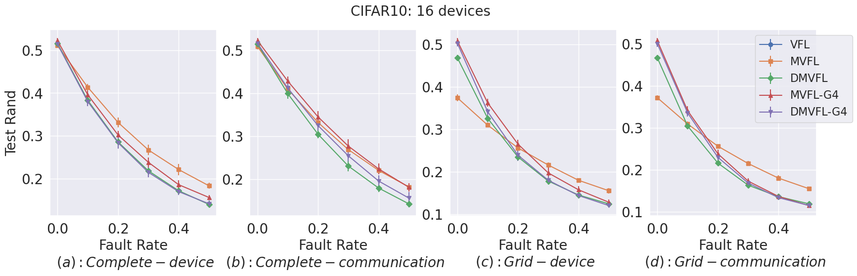
(b) Rand

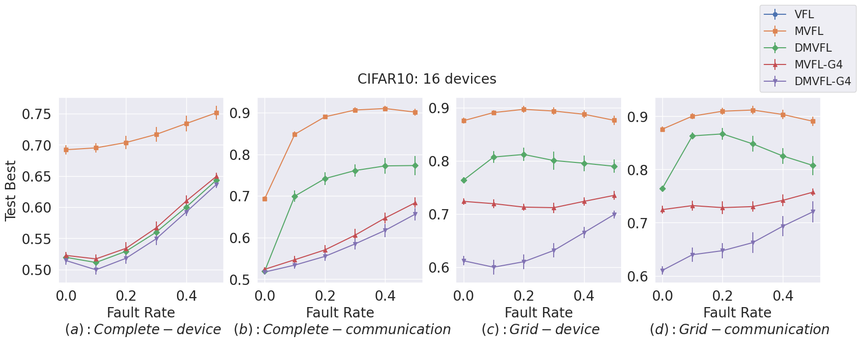
(c) Best

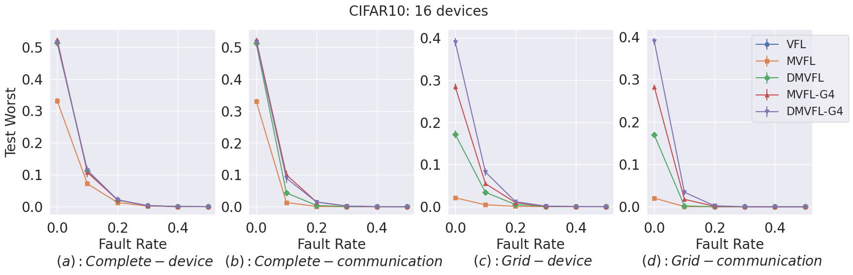
(d) Worst

Figure 19: All metrics reported for CIFAR-10 with 16 devices and only test time faults

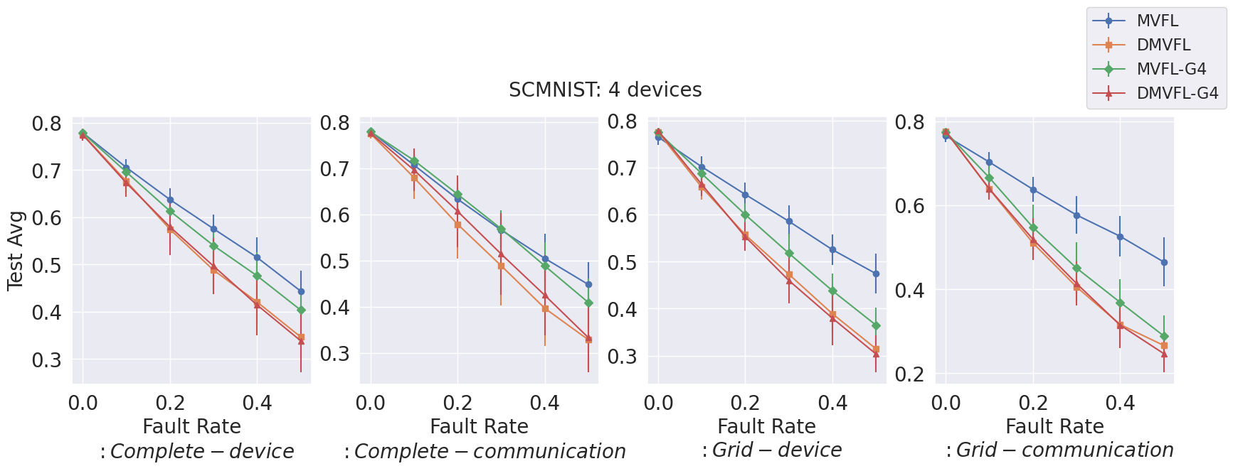
(a) 4 devices.

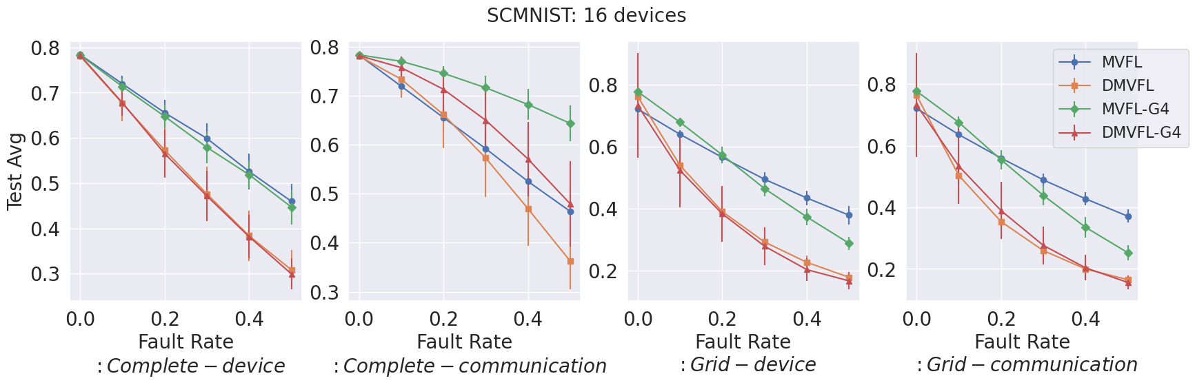
(b) 16 devices.

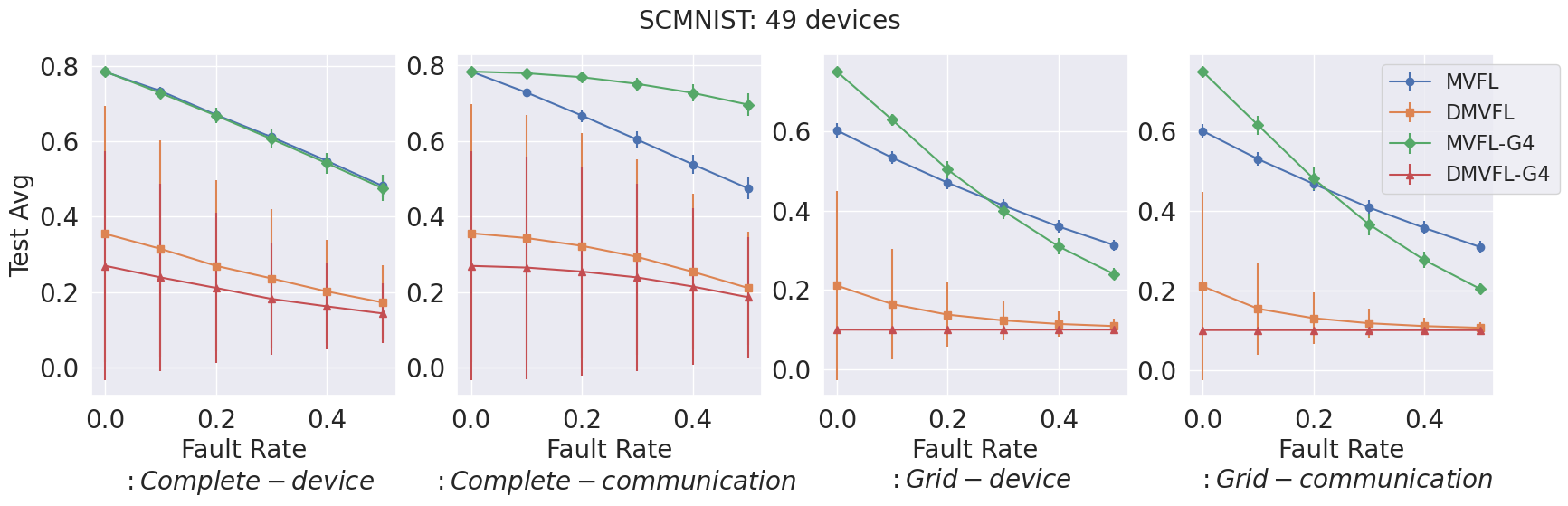
(c) 49 devices.

Figure 20: Test average accuracy under no train fault and different test time fault rates for StarCraftMNIST with 4,16 and 49 devices. Observing the plots it can be concluded that VFL does not do well under different faulting conditions and MVFL or its gossip variant has the best performance.

D.2 Training Faults

In Section 4.2 of the main paper we presented the effect of training fault on the test time performance under communication and device faulting regime. Here we present an extension by studying the average test time performance for 6 different rates of communication fault during training. Figures 9, 10 and 11 show the results for three datasets, MNIST, SCMNIST and CIFAR-10, respectively. Across the different sets and models it is observed that training with faults improves the average performance during test time faults. Furthermore, on observing Figures 9, 10 and 11 (c), it seems that gossiping has a profound impact on the model performance even if training with 100% faults, which means that each device is training it’s own local model independently. However, by doing gossip during the testing time, devices are able to reach a consensus that gives the model a performance boost, even during high testing fault rates.

D.3 Ablation Studies

Effect of number of communication rounds in DMVFL

In Section 3 of the main paper, we highlighted that the depth of DMVFL model is a hyperparameter. In Figures 12, 13 and 14 we present the investigation the effect of changing the depth hyperparameter for the three different datasets. The evaluation is carried out for average performance under no train faults but only test time faults with 16 devices.

Based on the figures we conclude that increasing the number for depths in DMVFL, does not have a favorable impact on average performance. We conjecture that this happens as per design, irrespective of the depth, we need to keep the total number of parameters the same for all the models, thus deeper DMVFL requires more communication and could receive more faulted information due to lack of parameters, resulting in inferior performance.

Effect of number of gossip rounds:

For the gossip (G) variants of MVFL and DMVFL-D2 methods, we are interested in studying the effect the number of gossip rounds has on average performance. In Figures 15 and 16 the effect of three different gossip rounds on the average performance for three different datasets is presented. From the plots we observe that irrespective of the method, Complete-communication train fault benefits the most with incorporating gossip rounds. Despite Grid-communication being a communication type of fault, gossiping does not improve the average performance. We believe this happens as a grid graph is quite sparse and training faults makes it more sparse. As a result, increasing gossip rounds does not lead to efficient passing of feature information from one client to another due to the sparseness, this is not the case in a complete graph. Furthermore, for reasons mentioned in Section 4.2 of the main paper, from Figures 15 and 16 we observe that adding any gossip rounds with device faults does not help in improving the performance.

D.4 Other metrics

In Figures 18,17 and 19 we present not only the average metric but also Rand, Best and Worst metrics when evaluation are carried out for 16 Devices/Clients under only test faults. In the main paper, Table 1 is a subset of the comprehensive data presented here.

D.5 Evaluation for different number of devices/clients

In Figure 20 we present average performance as a function of test time faults for three different number of devices. For all the different cases, it is observed that MVFL or its gossip variant performs the best. On observing the Complete-Communication plots for Figure 20, it can be seen that MVFL with gossiping has a more significant impact when the number of devices are 49 or 16 compared to when the number of devices are 4.

References

- Baran, [1964] Baran, P. (1964). On Distributed Communications: I. Introduction to Distributed Communications Networks. RAND Corporation, Santa Monica, CA.
- Belilovsky et al., [2019] Belilovsky, E., Eickenberg, M., and Oyallon, E. (2019). Greedy layerwise learning can scale to imagenet. In International conference on machine learning, pages 583–593. PMLR.
- Belilovsky et al., [2020] Belilovsky, E., Eickenberg, M., and Oyallon, E. (2020). Decoupled greedy learning of cnns. In International Conference on Machine Learning, pages 736–745. PMLR.
- Chen et al., [2020] Chen, T., Jin, X., Sun, Y., and Yin, W. (2020). Vafl: a method of vertical asynchronous federated learning. arXiv preprint arXiv:2007.06081.
- Chen et al., [2021] Chen, Z., Liao, W., Hua, K., Lu, C., and Yu, W. (2021). Towards asynchronous federated learning for heterogeneous edge-powered internet of things. Digital Communications and Networks, 7(3):317–326.
- Czarnecki et al., [2017] Czarnecki, W. M., Świrszcz, G., Jaderberg, M., Osindero, S., Vinyals, O., and Kavukcuoglu, K. (2017). Understanding synthetic gradients and decoupled neural interfaces. In Precup, D. and Teh, Y. W., editors, Proceedings of the 34th International Conference on Machine Learning, volume 70 of Proceedings of Machine Learning Research, pages 904–912. PMLR.
- Davies, [1966] Davies, D. W. (1966). Proposal for a digital communication network. Unpublished memo.
- Detorakis et al., [2018] Detorakis, G., Bartley, T., and Neftci, E. (2018). Contrastive hebbian learning with random feedback weights. CoRR, abs/1806.07406.
- Feng et al., [2021] Feng, C., Liu, B., Yu, K., Goudos, S. K., and Wan, S. (2021). Blockchain-empowered decentralized horizontal federated learning for 5g-enabled uavs. IEEE Transactions on Industrial Informatics, 18(5):3582–3592.
- Gabrielli et al., [2023] Gabrielli, E., Pica, G., and Tolomei, G. (2023). A survey on decentralized federated learning. arXiv preprint arXiv:2308.04604.
- Gu et al., [2021] Gu, X., Huang, K., Zhang, J., and Huang, L. (2021). Fast federated learning in the presence of arbitrary device unavailability. Advances in Neural Information Processing Systems, 34:12052–12064.
- Hegedűs et al., [2019] Hegedűs, I., Danner, G., and Jelasity, M. (2019). Gossip learning as a decentralized alternative to federated learning. In Distributed Applications and Interoperable Systems: 19th IFIP WG 6.1 International Conference, DAIS 2019, Held as Part of the 14th International Federated Conference on Distributed Computing Techniques, DisCoTec 2019, Kongens Lyngby, Denmark, June 17–21, 2019, Proceedings 19, pages 74–90. Springer.
- Hinton, [2022] Hinton, G. (2022). The forward-forward algorithm: Some preliminary investigations. arXiv preprint arXiv:2212.13345.
- Høier et al., [2023] Høier, R., Staudt, D., and Zach, C. (2023). Dual propagation: Accelerating contrastive hebbian learning with dyadic neurons.
- Kulinski et al., [2023] Kulinski, S., Waytowich, N. R., Hare, J. Z., and Inouye, D. I. (2023). Starcraftimage: A dataset for prototyping spatial reasoning methods for multi-agent environments. In Proceedings of the IEEE/CVF Conference on Computer Vision and Pattern Recognition, pages 22004–22013.
- Lalitha et al., [2019] Lalitha, A., Kilinc, O. C., Javidi, T., and Koushanfar, F. (2019). Peer-to-peer federated learning on graphs. arXiv preprint arXiv:1901.11173.
- Li et al., [2020] Li, M., Chen, Y., Wang, Y., and Pan, Y. (2020). Efficient asynchronous vertical federated learning via gradient prediction and double-end sparse compression. In 2020 16th international conference on control, automation, robotics and vision (ICARCV), pages 291–296. IEEE.
- Li et al., [2023] Li, S., Yao, D., and Liu, J. (2023). Fedvs: Straggler-resilient and privacy-preserving vertical federated learning for split models. arXiv preprint arXiv:2304.13407.
- Liu et al., [2021] Liu, Y., Qu, Y., Xu, C., Hao, Z., and Gu, B. (2021). Blockchain-enabled asynchronous federated learning in edge computing. Sensors, 21(10):3335.
- McMahan et al., [2017] McMahan, B., Moore, E., Ramage, D., Hampson, S., and y Arcas, B. A. (2017). Communication-efficient learning of deep networks from decentralized data. In Artificial intelligence and statistics, pages 1273–1282. PMLR.
- Movellan, [1991] Movellan, J. R. (1991). Contrastive hebbian learning in the continuous hopfield model. In Touretzky, D. S., Elman, J. L., Sejnowski, T. J., and Hinton, G. E., editors, Connectionist Models, pages 10–17. Morgan Kaufmann.
- Ruan et al., [2021] Ruan, Y., Zhang, X., Liang, S.-C., and Joe-Wong, C. (2021). Towards flexible device participation in federated learning. In International Conference on Artificial Intelligence and Statistics, pages 3403–3411. PMLR.
- Scarselli et al., [2008] Scarselli, F., Gori, M., Tsoi, A. C., Hagenbuchner, M., and Monfardini, G. (2008). The graph neural network model. IEEE transactions on neural networks, 20(1):61–80.
- Tang et al., [2022] Tang, Z., Shi, S., Li, B., and Chu, X. (2022). Gossipfl: A decentralized federated learning framework with sparsified and adaptive communication. IEEE Transactions on Parallel and Distributed Systems, 34(3):909–922.
- Thakur et al., [2019] Thakur, D., Kumar, Y., Kumar, A., and Singh, P. K. (2019). Applicability of wireless sensor networks in precision agriculture: A review. Wireless Personal Communications, 107:471–512.
- van Dijk et al., [2020] van Dijk, M., Nguyen, N. V., Nguyen, T. N., Nguyen, L. M., Tran-Dinh, Q., and Nguyen, P. H. (2020). Asynchronous federated learning with reduced number of rounds and with differential privacy from less aggregated gaussian noise. arXiv preprint arXiv:2007.09208.
- Wang and Ji, [2022] Wang, S. and Ji, M. (2022). A unified analysis of federated learning with arbitrary client participation. Advances in Neural Information Processing Systems, 35:19124–19137.
- Wu et al., [2022] Wu, Z., Li, Q., and He, B. (2022). Practical vertical federated learning with unsupervised representation learning. IEEE Transactions on Big Data.
- Zhang et al., [2021] Zhang, Q., Gu, B., Deng, C., and Huang, H. (2021). Secure bilevel asynchronous vertical federated learning with backward updating. In Proceedings of the AAAI Conference on Artificial Intelligence, volume 35, pages 10896–10904.