Robust Boundary Stabilization of Stochastic Hyperbolic PDEs

Abstract

This paper proposes a backstepping boundary control design for robust stabilization of linear first-order coupled hyperbolic partial differential equations (PDEs) with Markov-jumping parameters. The PDE system consists of 4 $\times$ 4 coupled hyperbolic PDEs whose first three characteristic speeds are positive and the last one is negative. We first design a full-state feedback boundary control law for a nominal, deterministic system using the backstepping method. Then, by applying Lyapunov analysis methods, we prove that the nominal backstepping control law can stabilize the PDE system with Markov jumping parameters if the nominal parameters are sufficiently close to the stochastic ones on average. The mean-square exponential stability conditions are theoretically derived and then validated via numerical simulations.

I Introduction

Hyperbolic partial differential equations (PDEs) find applications in many engineering areas, including transportation systems [21], open-channel flows [10]. Extensive research efforts have been made for boundary control problems of hyperbolic PDE systems. PDE backstepping, as a feedback stabilization method, has been developed for general first-order coupled hyperbolic PDEs in a series of work [9, 11, 15]. Further advances generalize the PDE backstepping for adaptive control [2], robust stabilization to delay and disturbances [3, 17]. These research results mainly pertain to deterministic PDE systems. On the other hand, scarce studies focus on stochastic PDE systems, the stochasticity being usually caused by uncertain parameters in real applications. The question of boundary control of uncertain hyperbolic PDEs with Markov jump parameters via the backstepping method remains open.

Previous results have focused on stochastic stability analysis with distributed or boundary controllers using linear matrix inequalities [1, 7, 12]. Prieur [18] modeled the abrupt changes of boundary conditions as a piecewise constant function and derived sufficient conditions for the exponential stability of the switching system. Wang et al. [20] examined the robustly stochastically exponential stability and stabilization of uncertain linear first-order hyperbolic PDEs with Markov jumping parameters, deriving sufficient stability conditions using linear matrix inequalities (LMIs) based on integral-type stochastic Lyapunov functional. Zhang [22] studied traffic flow control of Markov jump hyperbolic systems, employing LMIs to derive sufficient conditions for boundary exponential stability. Auriol [5] first considered the mean-square exponential stability of a $2\times 2$ stochastic hyperbolic system using backstepping.

The main results of this paper are that we propose a robust stabilizing backstepping control law for a $4\times 4$ stochastic hyperbolic PDEs. We first design a backstepping boundary control law to stabilize the nominal system without Markov jumping parameters. We prove that the nominal control law can still stabilize the stochastic PDE system, provided the nominal parameters are sufficiently close to the stochastic ones on average. The stability conditions are derived using a Lyapunov analysis. The contribution of this paper extends to both theoretical advancements and practical applications.

This paper is organized as follows: In Section II, we introduce the stochastic hyperbolic PDE system and state the problem under consideration. In Section III, the nominal boundary controller is designed, and the mean-square exponential stabilization of the stochastic PDEs is proposed. In Section IV, a Lyapunov analysis is conducted to prove the nominal control law achieves the mean-square exponential stability of the PDE system with Markov jumping parameters. In Section V numerical simulations verify the theoretical results.

II Problem Statement

In this paper, we consider the following stochastic PDE system

$$\mathbf{w}_{t}^{+}(x,t)+\Lambda^{+}(t)\mathbf{w}^{+}_{x}(x,t)= \Sigma^{++}(x,t)\mathbf{w}^{+}(x,t)$$

$$+\Sigma^{+-}(x,t)\mathbf{w}^{-}(x,t),$$ (1)

$$\mathbf{w}^{-}_{t}(x,t)-\Lambda^{-}(t)\mathbf{w}^{-}_{x}(x,t)= \Sigma^{-+}(x,t)\mathbf{w}^{+},$$ (2)

with the boundary conditions

$${\mathbf{w}^{+}(0,t)}={Q}(t)\mathbf{w}^{-}(0,t),$$ (3)

$$\mathbf{w}^{-}(1,t)={R}(t)\mathbf{w}^{+}(1,t)+{U}(t),$$ (4)

where $\mathbf{w}^{+}=[w_{1},w_{2},w_{3}]^{\mathsf{T}}$, $\mathbf{w}^{-}=w_{4}$, where the spatial and time domain are defined in $(x,t)\in[0,1]\times\mathbb{R}^{+}$. The different transport matrices are defined as

$$\Lambda^{+}(t)=\begin{bmatrix}\lambda_{1}(t)&0&0\\ 0&\lambda_{2}(t)&0\\ 0&0&\lambda_{3}(t)\end{bmatrix},\Lambda^{-}_{i}=\lambda_{4}(t)$$

The coefficient matrices are $\Sigma^{++}(x,t)\in\mathbb{R}^{3\times 3}$, $\Sigma^{+-}(x,t)\in\mathbb{R}^{1\times 3}$, $\Sigma^{-+}(x,t)\in\mathbb{R}^{3\times 1}$, ${Q}(t)\in\mathbb{R}^{3\times 1}$, ${R}(t)\in\mathbb{R}^{1\times 3}$. The function $U(t)$ is the control input. All the parameters of the systems are stochastic and we denote their concatenation $\mathscr{X}(t)=\{\Lambda^{+}(t),\Lambda^{-}(t),\Sigma^{++}(x,t),\Sigma^{+-}(x,t),\Sigma^{-+}(x,t),Q(t),R(t)\}$. We consider that the set $\mathscr{X}(t)$ corresponds to a homogeneous continuous Markov process $\mathscr{X}(t),t\in\mathbb{R}^{+}$ with a finite number of states $\mathscr{S}=\{\mathscr{X}_{1},\mathscr{X}_{2},\dots,\mathscr{X}_{r}\}$, whose realization is right continuous. For instance, we have $\mathscr{X}_{j}=\{\Lambda_{j}^{+},\Lambda_{j}^{-},\Sigma_{j}^{++}(x),\Sigma_{j}^{+-}(x),\Sigma_{j}^{-+}(x),Q_{j},R_{j}\}$.

The transition probabilities $P_{ij}(t_{1},t_{2})$ denote the probability to switch from mode $\mathscr{X}_{i}$ at time $t_{1}$ to mode $\mathscr{X}_{j}$ at time $t_{2}$ ($(i,j)\in\{1,\dots,r\}^{2},~{}0\leq t_{1}\leq t_{2}$). They satisfy  $P_{ij}:\mathbb{R}^{2}\rightarrow[0,1]$ with $\sum_{j=1}^{r}P_{ij}(t_{1},t_{2})=1$. Moreover, for $\varrho<t$, the transition probabilities ${P}_{ij}$ follows the Kolmogorov equation [14, 16],

$$\partial_{t}{P}_{ij}(\varrho,t)=-\mathfrak{c}_{j}(t){P}_{ij}(\varrho,t)+\sum_{k=1}^{r}{P}_{ik}(\varrho,t)\tau_{kj}(t),$$

$${P}_{ii}(\varrho,\varrho)=1,\text{ and }{P}_{ij}(\varrho,\varrho)=0\text{ for }i\neq j$$ (5)

where the $\tau_{ij}$ and $\mathfrak{c}_{j}=\sum_{k=1,k\neq j}^{r}\tau_{jk}$ are non-negative-valued functions such that $\tau_{ii}(t)=0$. The functions $\tau_{ij}$ are upper bounded by a constant $\tau^{\star}$. For $\mathscr{X}_{j}\in\mathscr{S}$, we denote $||\mathscr{X}_{j}(t)||$ as

$$||\mathscr{X}_{j}(t)|| =(||\Lambda^{+}_{j}(t)||^{2}+||\Lambda^{-}_{j}(t)||^{2}+||Q_{j}(t)||^{2}+||R_{j}(t)||^{2}$$

$$+\sup_{x\in[0,1]}||\Sigma_{j}^{++}(x)||^{2}+\sup_{x\in[0,1]}||\Sigma_{j}^{+-}(x)||^{2}$$

$$+\sup_{x\in[0,1]}||\Sigma_{j}^{-+}(x)||^{2})^{\frac{1}{2}},$$ (6)

where we have used the standard Euclidean norm. We assume that there exists known lower bounds $\underline{\mathscr{X}}$ and upper bounds $\overline{\mathscr{X}}$ such that for all $j$ , $\underline{\mathscr{X}}\leq||\mathscr{X}_{j}||\leq\overline{\mathscr{X}}$. Moreover, we assume that the lower bounds of the stochastic velocities are always positive. More precisely, we have $\underline{\Lambda_{i}^{+}}>0$, $\underline{\Lambda_{i}^{-}}>0$, which implies $\underline{\lambda_{1i}}>0$, $\underline{\lambda_{2i}}>0$, $\underline{\lambda_{3i}}>0$ and $\underline{\lambda_{4i}}>0$. Using the notations $\mathbf{w}=[\mathbf{w}^{+},\mathbf{w}^{-}]$ and $\Lambda_{i}=\text{Diag}\{\lambda_{1}^{i},\lambda_{2}^{i},\lambda_{3}^{i},-\lambda_{4}^{i}\}$, the system (1)-(4) can be rewritten in the compact form:

$$\partial_{t}\mathbf{w}(x,t)+\Lambda_{i}\partial_{x}\mathbf{w}(x,t)=\Theta_{i}\mathbf{w}(x,t),$$ (7)

for $x\in(0,L)$, with the boundary condition:

$$\left[\begin{array}[]{l}\mathbf{w}^{+}(0,t)\\ \mathbf{w}^{-}(1,t)\end{array}\right]=G_{i}\left[\begin{array}[]{l}\mathbf{w}^{+}(1,t)\\ \mathbf{w}^{-}(0,t)\end{array}\right]+\left[\begin{array}[]{c}0\\ {U}(t)\end{array}\right],$$ (14)

where the coefficient matrix $\Theta_{i}$, $G_{i}$ are:

$$\Theta_{i}=\left[\begin{array}[]{cc}\Sigma^{++}_{i}(x)&\Sigma^{+-}_{i}(x)\\ \Sigma^{-+}_{i}(x)&0\end{array}\right],G_{i}=\left[\begin{array}[]{cc}0&Q_{i}\\ R_{i}&0\end{array}\right].$$

In the case of deterministic coefficients, equations (7)-(14) naturally appear when modeling traffic networks with two classes of vehicles [8].

III Backstepping Controller Design

In this section, we propose a backstepping control design for the nominal system (that is, the system is in a known nominal deterministic state). We will then show that the stochastic system with this nominal control law is well-posed. Finally, we will state our main result, which is the mean-square exponential stability of the closed-loop system, provided the nominal parameters are sufficiently close to the stochastic ones on average. This result will be proved in the next section using a Lyapunov analysis.

III-A Backstepping transformation

We consider in this section that the stochastic parameters are in the nominal mode $\mathscr{X}(t)=\mathscr{X}_{0}$. This nominal mode is not necessarily related to the set $\mathscr{S}$. Our objective is to design a control law that stabilizes this nominal system. We first simplify the structure of the system (7) by removing the in-domain coupling terms in the equation. More precisely, let us consider the following backstepping transformation $\mathcal{K}_{0}$

$$\mathcal{K}_{0}\mathbf{w}=\begin{pmatrix}\mathbf{w}^{+}\\ \mathbf{w}^{-}-\int_{0}^{x}\mathbf{K}_{0}(x,\xi)\mathbf{w}^{+}(\xi,t)+N_{0}(x,\xi)\mathbf{w}^{-}(\xi,t))d\xi\end{pmatrix}$$ (15)

where the kernels $\mathbf{K}_{0}(x,\xi)\in\mathbb{R}^{1\times 3}$ and $N_{0}(x,\xi)\in\mathbb{R}^{1}$ are piecewise continuous functions defined on the triangular domain $\mathcal{T}=\{0\leq\xi\leq x\leq 1\}$. We have

$$\mathbf{K}_{0}(x,\xi)=\left[\begin{array}[]{ccc}k^{0}_{1}(x,\xi)&k^{0}_{2}(x,\xi)&k^{0}_{3}(x,\xi)\end{array}\right].$$ (17)

The different kernels verify the following PDE system

$$-\Lambda^{-}_{0}(\mathbf{K}_{0})_{x}(x,\xi)+(\mathbf{K}_{0})_{\xi}(x,\xi)\Lambda^{+}_{0}=-\mathbf{K}_{0}(x,\xi)\Sigma^{++}_{0}(\xi)$$

$$-\Sigma^{-+}_{0}(\xi)N_{0}(x,\xi),$$ (18)

$$\Lambda^{-}_{0}(N_{0})_{x}(x,\xi)+\Lambda^{-}_{0}(N_{0})_{\xi}(x,\xi)=\mathbf{K}_{0}(x,\xi)\Sigma^{+-}_{0}(\xi),$$ (19)

with the boundary conditions

$$\left(-\Lambda^{-}_{0}\mathbf{I}_{3}-\Lambda^{+}_{0}\right)\mathbf{K}_{0}^{\mathsf{T}}(x,x) =\Sigma^{-+^{\mathsf{T}}}_{0}(x),$$ (20)

$$-\Lambda^{-}_{0}N_{0}(x,0)+\mathbf{K}_{0}(x,0)\Lambda^{+}_{0}{Q}_{0} =0,$$ (21)

where $\mathbf{I}_{3}$ is a $3\times 3$ identity matrix. The well-posedness of the kernel equations can be proved by adjusting the results from [15, Theorem 3.3]. The solutions of the kernel equations can be expressed by integration along the characteristic lines. Applying the method of successive approximations, we can then prove the existence and uniqueness of the solution to the kernel equations (18)-(21). Applying the backstepping transformation, we can define the target system state $\vartheta$ as

$$\vartheta=(\alpha_{1},\alpha_{2},\alpha_{3},\beta)=\mathcal{K}_{0}\mathbf{w}.$$

And we denote the augmented states $\mathscr{Q}=[\alpha_{1},\alpha_{2},\alpha_{3}]^{\mathsf{T}}$ The target system equations are given by:

$$\mathscr{Q}_{t}(x,t)+\Lambda^{+}_{0}\mathscr{Q}_{x}(x,t)=\Sigma^{++}_{0}(x)\mathscr{Q}(x,t)+\Sigma^{+-}_{0}(x)\beta(x,t)$$

$$+\int_{0}^{x}\mathbf{C}_{0}^{+}(x,\xi)\mathscr{Q}(\xi,t)d\xi+\int_{0}^{x}\mathbf{C}_{0}^{-}(x,\xi)\beta(\xi,t)d\xi,$$ (22)

$$\beta_{t}\left(x,t\right)-\Lambda^{-}_{0}\beta_{x}(x,t)=0,$$ (23)

with the boundary conditions:

$$\mathscr{Q}(0,t)= {Q}_{0}\beta(0,t),$$ (24)

$$\beta(1,t)= R_{0}\mathbf{w}^{+}(1,t)-\int_{0}^{1}\mathbf{K}_{0}(1,\xi)\mathbf{w}^{+}(\xi,t)$$

$$+N_{0}(1,\xi)\mathbf{w}^{-}(\xi,t))d\xi+\bar{U}(t).$$ (25)

where the coefficients $\mathbf{C}_{0}^{+}(x,\xi)\in\mathbb{R}^{3\times 3}$ and $\mathbf{C}_{0}^{-}(x,\xi)\in\mathbb{R}^{3\times 1}$ are bounded functions defined on the triangular domain $\mathcal{T}$. Their expressions can be found in [8]. Note that we still have the presence of $\mathbf{w}^{+}$ and $\mathbf{w}^{-}$ terms in equation (25), but this is not a problem since these terms will be removed using the control input. The transformation $\mathcal{K}_{0}$ is a Volterra transformation, therefore boundedly invertible. Consequently, the states $\mathbf{w}$ and $\vartheta$ have equivalent $L^{2}$ norms, i.e. there exist two constants $m_{\vartheta}>0$ and $M_{\vartheta}>0$ such that

$$m_{\vartheta}||\mathbf{w}||_{L^{2}}^{2} \leq||\vartheta||_{L^{2}}^{2}\leq M_{\vartheta}||\mathbf{w}||_{L^{2}}^{2}.$$ (26)

III-B Nominal control law and Lyapunov functional

From the nominal target system (22)-(25), we can easily design a stabilizing control law as [4]:

$${U}(t)= -{R}_{0}\mathbf{w}^{+}(1,t)+\int_{0}^{1}\left(\mathbf{K}_{0}(1,\xi)\mathbf{w}^{+}(\xi,t)\right.$$

$$\left.+N_{0}(1,\xi)\mathbf{w}^{-}(\xi,t)\right)d\xi.$$ (27)

To analyze the stability properties of the target system (22)-(25), we consider the Lyapunov functional $V_{0}$ defined by

$$V_{0}(t)=\int_{0}^{1}\vartheta^{\mathsf{T}}(x,t)D_{0}(x)\vartheta(x,t)dx,$$ (28)

where

$$D_{0}(x)=\text{Diag}\left\{\frac{\mathrm{e}^{-\frac{\nu}{\lambda_{1}^{0}}x}}{\lambda_{1}^{0}},\frac{\mathrm{e}^{-\frac{\nu}{\lambda_{2}^{0}}x}}{\lambda_{2}^{0}},\frac{\mathrm{e}^{-\frac{\nu}{\lambda_{3}^{0}}x}}{\lambda_{3}^{0}},a\frac{\mathrm{e}^{\frac{\nu}{\Lambda^{-}_{0}}x}}{\Lambda^{-}_{0}}\right\}.$$ (29)

This Lyapunov functional is equivalent to the $L^{2}$ norm of the system, that is, there exist two constant $k_{1}>0$ and $k_{2}>0$ such that

$$k_{1}||\vartheta||_{L^{2}}^{2}\leq V_{0}(t)\leq k_{2}||\vartheta||_{L^{2}}^{2}.$$ (30)

It can also be expressed in terms of the original state as

$$V_{0}(t)=\int_{0}^{1} (\mathcal{K}_{0}\mathbf{w}(x,t))^{\mathsf{T}}D_{0}(x)\mathcal{K}_{0}\mathbf{w}(x,t)dx.$$ (31)

Taking the time derivative of $V_{0}(t)$ and integrating by parts, we get

$$\dot{V}_{0}(t)\leq-\nu V_{0}(t)+\int_{0}^{1}2\mathscr{Q}(x,t)D_{\alpha}^{0}$$

$$\left(\Sigma_{0}^{++}(x)\mathscr{Q}(x,t)+\Sigma_{0}^{+-}(x)\mathbf{w}^{-}(x,t)\right)dx$$

$$\leq-\eta V_{0}(t)+(q_{10}^{2}+q_{20}^{2}+q_{30}^{2}-a)\beta^{2}(0,t),$$ (32)

where

$$\eta=\nu-\frac{2}{||\underline{\Lambda^{+}}||k_{1}}(\max_{x\in[0,1]}||\Sigma^{++}_{0}(x)||$$

$$+(1+\frac{1}{m_{\vartheta}})\max_{x\in[0,1]}||\Sigma^{+-}_{0}||(x)),$$ (33)

$$D_{\alpha}^{0}=\text{Diag}\left\{\frac{\mathrm{e}^{-\frac{\nu}{\lambda_{1}^{0}}x}}{\lambda_{1}^{0}},\frac{\mathrm{e}^{-\frac{\nu}{\lambda_{2}^{0}}x}}{\lambda_{2}^{0}},\frac{\mathrm{e}^{-\frac{\nu}{\lambda_{3}^{0}}x}}{\lambda_{3}^{0}}\right\}.$$ (34)

We choose $a>0$ and $\nu>0$ such that

$$q_{10}^{2}+q_{20}^{2}+q_{30}^{2}-a\leq 0,\eta>0.$$ (35)

where $q_{10}$, $q_{20}$, $q_{30}$ are the elements of $Q_{0}$. Consequently, we obtain $\dot{V}_{0}(t)\leq-\eta V_{0}(t)$, which implies the $L^{2}$-exponential stability of the system.

III-C Mean-square exponential stabilization

We now state the well-posedness of the stochastic system and then give the main result on mean-square exponential stability. We must first guarantee that the stochastic system (1)-(4) with the nominal controller (27) has a unique solution. We have the following lemma,

Lemma 1.

For any initial conditions of the Markov system $\mathbf{w}(x,t)\in L^{2}[0,1]$ and any initial states $\mathscr{X}(t)=\mathscr{X}(0)$ for the stochastic parameters, the system (1)-(4) with the nominal control law (27) has a unique solution such that for any $t$,

$$\mathbb{E}\{||\mathbf{w}(x,t)||\}<\infty,$$ (36)

where the $\mathbb{E}\{\cdot\}$ denotes the mathematical expectation.

Proof.

This lemma can be easily proved by adjusting the results in [22]. Almost every sample path of our stochastic processes are right-continuous step functions with a finite number of jumps in any finite time interval. We can then find a sequence $\{t_{k}:k=0,1,\dots\}$ of stopping times such that $t_{0}=0,\lim_{t\to\infty}t_{k}=\infty$, and $\mathscr{X}(t)=\mathscr{X}(t_{k})$ on $t_{k}\leq t<t_{k+1}$. We start from time $t=0$ and then use [6, Theorem A.4] for each time interval in the whole time period. Thus, the stochastic system (1)-(4) has a unique solution. ∎

The main goal of this paper is to prove that the control law (27) can still stabilize the stochastic system (1)-(4), provided the nominal parameter $\mathscr{X}_{0}$ is sufficiently close to the stochastic ones on average. More precisely, we want to show the following sufficient condition for robust stabilization.

Theorem 1.

There exists a constant $\epsilon^{\star}>0$, such that if, for all time $t>0$,

$$\mathbb{E}\left(\left|\left|\mathscr{X}(t)-\mathscr{X}_{0}\right|\right|\right)\leq\epsilon^{\star},$$ (37)

then the closed-loop system (1)-(4) with the control law (27) is mean-square exponentially stable, namely, there exist $\varsigma,\zeta>0$ such that:

$$\mathbb{E}_{[0,(p(0),\mathscr{X}(0)]}(p(t))\leq\varsigma\mathrm{e}^{-\zeta t}p(0),$$ (38)

where $p(t)=\int_{0}^{1}||\mathbf{w}(x,t)||_{2}^{2}dx$, while $\mathbb{E}_{[0,(p(0),\mathscr{X}(0)]}$ denotes the conditional expectation at time $t=0$ with initial settings of $p(t)=p(0)$, $\mathscr{X}(t)=\mathscr{X}(0)$.

This theorem will be proved in the next section.

IV Lyapunov Analysis

In this section, we consider the closed-loop stochastic system with the nominal controller (27). The objective is to prove Theorem 2. The proof will rely on a Lyapunov analysis. More precisely, we will consider the following stochastic Lyapunov functional candidate

$$V(t)=\int_{0}^{1} (\mathcal{K}_{0}\mathbf{w}(x,t))^{\mathsf{T}}D(t,x)\mathcal{K}_{0}\mathbf{w}(x,t)dx,$$ (39)

where the diagonal matrix $D(t,x)=D_{j}(x)$ if $\mathscr{X}(t)=\mathscr{X}_{j}$, and where

$$D_{j}(x)=\text{Diag}\left\{\frac{\mathrm{e}^{-\frac{\nu}{\lambda_{1}^{j}}x}}{\lambda_{1}^{j}},\frac{\mathrm{e}^{-\frac{\nu}{\lambda_{2}^{j}}x}}{\lambda_{2}^{j}},\frac{\mathrm{e}^{-\frac{\nu}{\lambda_{3}^{j}}x}}{\lambda_{3}^{j}},a\frac{\mathrm{e}^{\frac{\nu}{\Lambda^{-}_{j}}x}}{\Lambda^{-}_{j}}\right\}.$$ (40)

We consider that the parameters $\nu$ and $a$ introduced in the definition of $D_{j}$ can still be tuned. In the nominal case $\mathscr{X}(t)=\mathscr{X}_{0}$, the Lyapunov functional $V(t)$ corresponds to $V_{0}$. It is noted that inequality (30) still holds for $V(t)$ (even if the constants $k_{1}$ and $k_{2}$ may change).

IV-A Target system in stochastic mode $\mathscr{X}_{j}$

In this section, we consider that $\mathscr{X}(t)=\mathscr{X}_{j}$ at time $t$. We can define the state $\vartheta=(\alpha_{1},\alpha_{2},\alpha_{3},\beta)=\mathcal{K}_{0}\mathbf{w}$. Our objective is first to obtain the equations verified by the state $\vartheta$ that appears in the Lyapunov functional (39). It verifies the following set of equations

$$\mathscr{Q}_{t}(x,t)+\Lambda^{+}_{j}\mathscr{Q}_{x}(x,t)= \Sigma^{++}_{j}(x)\mathbf{w}^{+}(x,t)$$

$$+\Sigma^{+-}_{j}(x)\mathbf{w}^{-}(x,t),$$ (41)

$$\beta_{t}\left(x,t\right)-\Lambda^{-}_{j}\beta_{x}(x,t)=\mathbf{f}_{1j}(x)\mathbf{w}^{+}(x,t)+\mathbf{f}_{2j}(x)\beta(0,t)$$

$$+\int_{0}^{x}\mathbf{f}_{3j}(x,\xi)\mathbf{w}^{+}(\xi,t)d\xi+\int_{0}^{x}\mathbf{f}_{4j}(x,\xi)\mathbf{w}^{-}(\xi,t)d\xi,$$ (42)

with the boundary conditions:

$$\mathscr{Q}(0,t) ={Q}_{j}\beta(0,t),$$ (43)

$$\beta(1,t) =\left({R}_{j}-{R}_{0}\right)\mathscr{Q}(1,t),$$ (44)

where the functions are defined by:

$$\mathbf{f}_{1j}(x) =\Sigma^{-+}_{j}(x)+\Lambda^{-}_{j}\mathbf{K}_{0}(x,x)+\mathbf{K}_{0}(x,x)\Lambda^{+}_{j},$$ (45)

$$\mathbf{f}_{2j}(x) =-\mathbf{K}_{0}(x,0)\Lambda^{+}_{j}{Q}_{j}+N_{0}(x,0)\Lambda^{-}_{j},$$ (46)

$$\mathbf{f}_{3j}(x,\xi) =\Lambda^{-}_{j}(\mathbf{K}_{0})_{x}(x,\xi)-(\mathbf{K}_{0})_{\xi}(x,\xi)\Lambda^{+}_{j}$$

$$-\mathbf{K}_{0}(x,\xi)\Sigma^{++}_{j}(\xi)-N_{0}(x,\xi)\Sigma^{-+}_{j}(\xi),$$ (47)

$$\mathbf{f}_{4j}(x,\xi) =\Lambda^{-}_{j}(N_{0})_{x}(x,\xi)+\Lambda^{-}_{j}(N_{0})_{\xi}(x,\xi)$$

$$-\mathbf{K}_{0}(x,\xi)\Sigma^{+-}_{j}(\xi).$$ (48)

All the terms that depend on $\mathbf{w}$ in the target system (41)-(44) could be expressed in terms of $\vartheta$ using the inverse transformation $\mathcal{K}_{0}^{-1}$. However, this would make the computations more complex and is not required for the stability analysis. It is important to emphasize that all the terms on the right-hand side of equation (42) become small if the stochastic parameters are close enough to the nominal ones. More precisely, we have the following lemma

Lemma 2.

There exists a constant $M_{0}$, such that for any realization $\mathscr{X}(t)=\mathscr{X}_{j}\in\mathscr{S}$, for any $(x,\xi)\in\mathcal{T}$

$$||\mathbf{f}_{\mathfrak{i}j}||<M_{0}\left|\left|\mathscr{X}_{j}-\mathscr{X}_{0}\right|\right|,\quad\mathfrak{i}\in\{1,2,3,4\}.$$ (49)

Proof.

Considering the function $\mathbf{f}_{1j}(x)$. For all $x\in[0,1]$, we have

$$\mathbf{f}_{1j}(x) =\Sigma^{-+}_{j}(x)+\Lambda^{-}_{j}\mathbf{K}_{0}(x,x)+\mathbf{K}_{0}(x,x)\Lambda^{+}_{j}$$

$$=(\Sigma^{-+}_{j}(x)-\Sigma^{-+}_{0}(x))+(\Lambda^{-}_{j}-\Lambda^{-}_{0})\mathbf{K}_{0}(x,x)$$

$$+\mathbf{K}_{0}(x,x)(\Lambda^{+}_{j}-\Lambda^{+}_{0}).$$ (50)

Consequently, we obtain the existence of a constant $K_{1}>0$ such that

$$||\mathbf{f}_{1j}|| \leq K_{1}\left|\left|\mathscr{X}_{j}-\mathscr{X}_{0}\right|\right|.$$ (51)

The other inequalities for $\mathbf{f}_{2}(x)$, $\mathbf{f}_{3}(x,\xi)$ and $\mathbf{f}_{4}(x,\xi)$ can also be derived similarly. This finishes the proof. ∎

IV-B Derivation of the Lyapunov function

Let us consider the Lyapunov functional  $V$ defined in equation (39). Its infinitesimal generator $L$ is defined as [19]

$$LV(\mathbf{w},s_{2}) =\limsup_{\Delta t\rightarrow 0^{+}}\frac{1}{\Delta t}\times\mathbb{E}(V(\mathbf{w}(t+\Delta t),\mathscr{X}(t+\Delta t))$$

$$-V(\mathbf{w}(t),\mathscr{X}(t))).$$ (52)

We define $L_{j}$, the infinitesimal generator of $V$ obtained by fixing $\mathscr{X}(t)=\mathscr{X}_{j}\in\mathscr{S}$. We have

$$L_{j}V(\mathbf{w}) =\frac{dV}{d\mathbf{w}}\left(\vartheta,\mathscr{X}_{j}\right)h_{j}(\vartheta)+\sum_{\ell\in\mathscr{S}}\left(V_{\ell}(\mathbf{w})-V_{j}(\mathbf{w})\right)\tau_{j\ell},$$ (53)

where $V_{\ell}(\mathbf{w})=V(\mathbf{w},s_{2}^{\ell})$, and where the operator $h_{j}$ is defined by

$$h_{j}(\vartheta)=\left(\begin{array}[]{l}-\Lambda^{+}_{j}\mathscr{Q}_{x}(x,t)+\Sigma_{j}^{++}(x)\mathbf{w}^{+}(x,t)\\ +\Sigma_{j}^{+-}(x)\mathbf{w}^{-}(x,t)\\ \Lambda_{j}^{-}\beta_{x}(x,t)+\mathbf{f}_{1j}(x)\mathbf{w}^{+}(x,t)\\ +\mathbf{f}_{2j}(x)\beta(0,t)+\int_{0}^{x}\mathbf{f}_{3j}(x,\xi)\mathbf{w}^{+}(\xi,t)d\xi\\ +\int_{0}^{x}\mathbf{f}_{4j}(x,\xi)\mathbf{w}^{-}(\xi,t)d\xi\end{array}\right).$$ (59)

To shorten the computations, we denote in the sequel $V(t),LV(t),V_{j}(t)$ and $L_{j}V(t)$ instead of (respectively) $V(\mathbf{w},\mathscr{X}(t))$, $LV(\mathbf{w},\mathscr{X}(t))$, $V(\mathbf{w},\mathscr{X}_{j})$ and $L_{j}(V(\mathbf{w}))$. From now, we consider that $\mathscr{X}(t=0)=\mathscr{X}_{i_{0}}\in\mathscr{S}$. We have the following lemma.

Lemma 3.

There exists $\bar{\eta}>0$, $M_{1}>0$ and $d_{1},d_{2}>0$ such that the Lyapunov functional $V(t)$ satisfies

$$\sum_{j=1}^{r}P_{ij}(0,t)L_{j}V(t)\leq-V(t)\Bigg{(}\bar{\eta}-d_{1}\mathcal{Z}(t)$$

$$\left.-\left(M_{1}+d_{1}r\tau^{\star}\right)\mathbb{E}\left(\left|\left|\mathscr{X}(t)-\mathscr{X}_{0}\right|\right|\right)\right)$$

$$+\sum_{k=1}^{3}(d_{2}\mathbb{E}(\left|\left|\mathscr{X}(t)-\mathscr{X}_{0}\right|\right|)-\mathrm{e}^{-\frac{\nu}{\bar{\lambda}}})\alpha_{k}^{2}(1,t)$$ (60)

where the function $\mathcal{Z}(t)$ is defined as:

$$\mathcal{Z}(t)=\sum_{j=1}^{r}\left|\left|\mathscr{X}(t)-\mathscr{X}_{0}\right|\right|\left(\partial_{t}P_{ij}(0,t)+\mathfrak{c}_{j}P_{ij}(0,t)\right)$$ (61)

Proof.

In what follows, we denote $c_{i}$ positive constants. We will first compute the first term of $L_{j}$. Consider that $\mathscr{X}(t)=\mathscr{X}_{j}$. The Lyapunov functional rewrites

$$V_{j}(t)=\int_{0}^{1}\vartheta^{\mathsf{T}}(x,t)D_{j}(x)\vartheta(x,t)dx,$$ (62)

$$\frac{dV_{j}}{d\mathbf{w}}(\mathbf{w})h_{j}(\mathbf{w})\leq-\eta V_{j}(t)+M_{1}\left|\left|\mathscr{X}_{j}-\mathscr{X}_{0}\right|\right|V(t)$$

$$+\left(c_{2}\left|\overline{\mathscr{X}}-\underline{\mathscr{X}}\right|\varepsilon_{0}+q_{1j}^{2}+q_{2j}^{2}+q_{3j}^{2}-a\right)\beta^{2}(0,t)$$

$$+\sum_{k=1}^{3}(a\mathrm{e}^{\frac{\nu}{\Lambda^{-}_{j}}}\left(({R}_{j})_{k}-({R}_{0})_{k}\right)^{2}-\mathrm{e}^{-\frac{\nu}{\lambda_{kj}}L})\alpha_{k}^{2}(1,t),$$ (63)

where

$$\eta=\nu-\frac{2}{||\underline{\Lambda^{+}}||k_{1}}(\max_{x\in[0,1]}||\Sigma^{++}_{0}(x)||$$

$$+(1+\frac{1}{m_{\vartheta}})\max_{x\in[0,1]}||\Sigma^{+-}_{0}(x)||)-\frac{2\overline{\mathscr{X}}c_{2}}{k_{1}\varepsilon_{0}},$$ (64)

$$M_{1}=c_{4}+ac_{3}+\frac{c_{2}}{k_{1}\varepsilon_{0}}+c_{1}.$$ (65)

The coefficients $\nu$, $\varepsilon_{0}$ and $a$ are chosen such that

$$\eta>0,\quad c_{2}\left|\overline{\mathscr{X}}-\underline{\mathscr{X}}\right|\varepsilon_{0}+{q}_{1j}^{2}+{q}_{2j}^{2}+{q}_{3j}^{2}-a<0.$$ (66)

where the ${q}_{1j}$, ${q}_{2j}$, ${q}_{3j}$ are the elements of ${Q}_{j}$, $\overline{\mathscr{X}}$ and $\underline{\mathscr{X}}$ are the upper and lower bound of the stochastic parameters. There exists a constant $C_{0}$ such that for all $1\leq j\leq r$, $V_{j}(\mathbf{w})\leq C_{0}V(\mathbf{w})$. Thus, we get the following inequality:

$$\frac{dV_{j}}{d\mathbf{w}}(\mathbf{w})h_{j}(\mathbf{w})\leq-\bar{\eta}V(t)+M_{1}\left|\left|\mathscr{X}_{j}-\mathscr{X}_{0}\right|\right|V(t)$$

$$+\sum_{k=1}^{3}(a\mathrm{e}^{\frac{\nu}{\Lambda^{-}_{j}}}\left(({R}_{j})_{k}-({R}_{0})_{k}\right)^{2}-\mathrm{e}^{-\frac{\nu}{\lambda_{kj}}L})\alpha_{k}^{2}(1,t),$$ (67)

where $\bar{\eta}=\eta C_{0}$. Now, we calculate the second term of $L_{j}$. We have:

$$\sum_{l=1}^{r}\left(V_{l}(\mathbf{w})-V_{j}(\mathbf{w})\right)\tau_{jl}=\sum_{l=1}^{r}\tau_{jl}$$

$$\left(\int_{0}^{1}\mathcal{K}_{0}^{\mathsf{T}}(\mathbf{w}(x,t))D_{l}(x)\mathcal{K}_{0}\mathbf{w}(x,t)dx\right.$$

$$-\left.\int_{0}^{1}\mathcal{K}_{0}^{\mathsf{T}}\mathbf{w}(x,t)D_{j}(x)\mathcal{K}_{0}\mathbf{w}(x,t)dx\right).$$

$$\leq d_{1}\sum_{l=1}^{r}\tau_{jl}\left|\left|\mathscr{X}_{l}-\mathscr{X}_{j}\right|\right|V(t),$$ (68)

We then calculate the quantity $\bar{L}=\sum_{j=1}^{r}P_{ij}(0,t)L_{j}V(t)$. Using the property of the expectation and we get

$$\bar{L}\leq-V(t)\left(\bar{\eta}-(M_{1}+d_{1}r\tau^{\star})\mathbb{E}(\left|\left|\mathscr{X}(t)-\mathscr{X}_{0}\right|\right|)\right.$$

$$\left.+d_{1}\sum_{j=1}^{r}\left|\left|\mathscr{X}_{j}-\mathscr{X}_{0}\right|\right|\left(\partial_{t}P_{ij}(0,t)+\mathfrak{c}_{j}P_{ij}(0,t)\right)\right)$$

$$+\sum_{k=1}^{3}(d_{2}\mathbb{E}(\left|\left|\mathscr{X}(t)-\mathscr{X}_{0}\right|\right|)-\mathrm{e}^{-\frac{\nu}{\bar{\lambda}}})\alpha_{k}^{2}(1,t),$$ (69)

This finish the proof of Lemma 3. ∎

IV-C Proof of Theorem 2

Notice first that if $\epsilon^{\star}$ is small enough (namely smaller than $\frac{e^{-\frac{\nu}{\bar{\lambda}}}}{d_{2}}$) and if inequality (37) holds, the term $\sum_{k=1}^{3}(d_{2}\mathbb{E}(\left|\left|\mathscr{X}(t)-\mathscr{X}_{0}\right|\right|)-\mathrm{e}^{-\frac{\nu}{\bar{\lambda}}})\alpha_{k}^{2}(1,t)<0$, then we have the following result based on Lemma 3:

$$\sum_{j=1}^{r}P_{ij}(0,t)L_{j}V(t)\leq-V(t)\Bigg{(}\bar{\eta}-d_{1}\mathcal{Z}(t)$$

$$\left.-\left(M_{1}+d_{1}r\tau^{\star}\right)\mathbb{E}\left(\left|\left|\mathscr{X}(t)-\mathscr{X}_{0}\right|\right|\right)\right).$$ (70)

We define the following function:

$$\phi(t)=\bar{\eta}-d_{1}\mathcal{Z}(t)-(M_{1}+d_{1}r\tau^{\star})\mathbb{E}(||\mathscr{X}(t)-\mathscr{X}_{0}||).$$ (71)

And then, using the functional $\Psi(t)$:

$$\Psi(t)=\mathrm{e}^{\int_{0}^{t}\phi(y)dy}V(t).$$ (72)

With the definition of $\Psi(t)$, taking the expectation of the infinitesimal generator $L$ of $\Psi(t)$ , we get:

$$\mathbb{E}\left(\sum_{j=1}^{r}P_{ij}(0,t)L_{j}V(t)\right)\leq-\mathbb{E}\left(V(t)\phi(t)\right).$$ (73)

We know that $\mathbb{E}(\sum_{j=1}^{r}P_{ij}(0,t)L_{j}V(t))=\mathbb{E}(LV(t))$, thus

$$\mathbb{E}(LV(t))\leq-\mathbb{E}(V(t)\phi(t)).$$ (74)

Then applying the Dynkin’s formula [13],

$$\mathbb{E}(\Psi(t))-\Psi(0)=\mathbb{E}\left(\int_{0}^{t}L\Psi(y)dy\right)\leq 0.$$ (75)

To calculate the $\mathbb{E}(\Psi(t))$, we write down the formulation of $\Psi(t)$:

$$\mathbb{E}(\Psi(t))=\mathbb{E}\left(V(t)\mathrm{e}^{\int_{0}^{t}\phi(y)dy}\right)$$

$$=\mathbb{E}\left(V(t)\mathrm{e}^{\int_{0}^{t}(\bar{\eta}-d_{1}\mathcal{Z}(y)-(M_{1}+d_{1}r\tau^{*})\mathbb{E}(||\mathscr{X}(y)-\mathscr{X}_{0}||))dy}\right).$$ (76)

We already know that

$$\int_{0}^{t}\mathcal{Z}(y)dy=\int_{0}^{t}\left(\sum_{j=1}^{r}\left|\left|\mathscr{X}(y)-\mathscr{X}_{0}\right|\right|\left(\partial_{y}P_{ij}(0,y)\right.\right.$$

$$\left.+\mathfrak{c}_{j}P_{ij}(0,y)\right)V(y)\Big{)}dy$$

$$\leq\mathbb{E}(\left|\left|\mathscr{X}(t)-\mathscr{X}_{0}\right|\right|)+r\tau^{\star}\int_{0}^{t}\mathbb{E}(\left|\left|\mathscr{X}(y)-\mathscr{X}_{0}\right|\right|)dy,$$ (77)

where $\tau^{\star}$ is the largest value of the transition rate. Using this inequality, we get

$$\mathbb{E}(\Psi(t))\geq\mathbb{E}\left(V(t)\mathrm{e}^{\left(-d_{1}\epsilon^{\star}+\int_{0}^{t}(\bar{\eta}-(M_{1}+2d_{1}r\tau^{\star})\epsilon^{\star}dy\right)}\right).$$ (78)

Then we take $\epsilon^{\star}$ as

$$\epsilon^{\star}=\frac{\bar{\eta}}{2(2d_{1}r\tau^{\star}+M_{1})},$$ (79)

thus we have

$$\mathbb{E}(\Psi(t))\geq\mathbb{E}\left(V(t)\mathrm{e}^{\left(-d_{1}\epsilon^{\star}+\frac{\bar{\eta}}{2}t\right)}\right).$$ (80)

From the before proof, we know $\mathbb{E}(\Psi(t))\leq\Psi(0)$, such that

$$\mathbb{E}(V(t))\leq\mathrm{e}^{d_{1}\epsilon^{\star}}\mathrm{e}^{-\zeta t}V(0),$$ (81)

where $\zeta=\frac{\bar{\eta}}{2}$. The function $V(t)$ is equivalent to the $L^{2}$-norm of the system. This concludes the proof of Theorem 1.

V Numerical Simulation

In this section, we illustrate our results with simulations. We consider that only the parameter $\lambda_{4}$ is stochastic. Its nominal value is $-0.024$. The five other possible values are $\lambda_{4}^{1}=-0.02,\lambda_{4}^{2}=-0.023,\lambda_{4}^{3}=-0.024,\lambda_{4}^{4}=-0.025,\lambda_{4}^{5}=-0.03)$ and the initial transition probabilities are chosen as $(0.02,0.32,0.32,0.32,0.02)$. The transition rates $\tau_{ij}$ are defined as the same as in  [5]. The corresponding matrices in nominal case are setting as:

$$\Lambda^{+}_{0}=\left[\begin{array}[]{ccc}0.0081&0&0\\ 0&0.0037&0\\ 0&0&0.0065\end{array}\right],\Lambda^{-}_{0}=-0.024$$

$$Q_{0}=\begin{bmatrix}-12.29\\ -3\\ 8.45\end{bmatrix},R_{0}=\begin{bmatrix}0.0011&-0.1601&0.0034\end{bmatrix}$$

Solving the Kolmogorov forward equation, we get the probability of each state in the simulation process shown in Fig. 1.

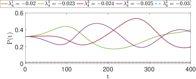
Figure 1: The probability of Markov states

From the probability of the Markov states, the system stays near the nominal value in the entire simulation period. Using the Markov process, we conduct the simulation for $t=400$ with the sinusoidal initial conditions, the closed-loop results are shown in Fig. 2.

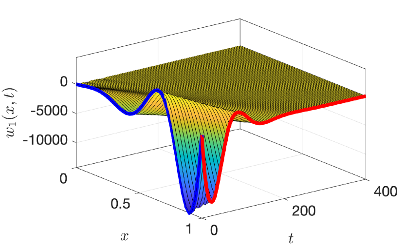
(a) $w_{1}$

(b) $w_{2}$

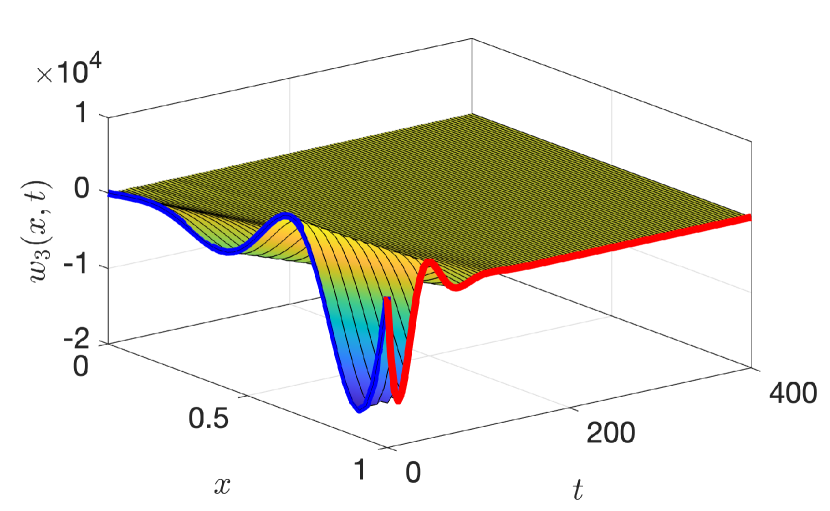
(c) $w_{3}$

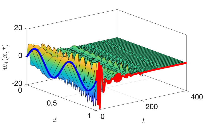
(d) $w_{4}$

Figure 2: Closed-loop results of the stochastic system

All the states with Markov jumping parameters almost converge to zero under the nominal control law, which is consistent with the theoretical results.

VI Conclusions

In this paper, we proposed a backstepping control low that mean-squarely exponentially stabilizes a $4\times 4$ Markov jumping coupled hyperbolic PDEs. The full-state feedback boundary control law was derived using the backstepping method for a nominal system. By applying Lyapunov analysis, we prove that this nominal control law can stabilize the PDE system with Markov jumping parameters provided the nominal parameters are sufficiently close to the stochastic ones on average. Finally, we use numerical examples to illustrate the efficiency of our approach.Future work will focus on its application in traffic flow systems.

References

• [1] S. Amin, F. M. Hante, and A. M. Bayen. Exponential stability of switched linear hyperbolic initial-boundary value problems. IEEE Transactions on Automatic Control, 57(2):291–301, 2011.
• [2] H. Anfinsen and O. M. Aamo. Adaptive control of linear2$\times$ 2 hyperbolic systems. Automatica, 87:69–82, 2018.
• [3] J. Auriol, U. J. F. Aarsnes, P. Martin, and F. Di Meglio. Delay-robust control design for two heterodirectional linear coupled hyperbolic pdes. IEEE Transactions on Automatic Control, 63(10):3551–3557, 2018.
• [4] J. Auriol and F. Di Meglio. Minimum time control of heterodirectional linear coupled hyperbolic pdes. Automatica, 71:300–307, 2016.
• [5] J. Auriol, M. Pereira, and B. Kulcsar. Mean-square exponential stabilization of coupled hyperbolic systems with random parameters. IFAC-PapersOnLine, pages 8823–8828, 2023.
• [6] G. Bastin and J.-M. Coron. Stability and boundary stabilization of 1-d hyperbolic systems, volume 88. Springer, 2016.
• [7] P. Bolzern, P. Colaneri, and G. De Nicolao. On almost sure stability of continuous-time markov jump linear systems. Automatica, 42(6):983–988, 2006.
• [8] M. Burkhardt, H. Yu, and M. Krstic. Stop-and-go suppression in two-class congested traffic. Automatica, 125:109381, 2021.
• [9] J.-M. Coron, R. Vazquez, M. Krstic, and G. Bastin. Local exponential $h^{2}$ stabilization of a 2$\times$2 quasilinear hyperbolic system using backstepping. SIAM Journal on Control and Optimization, 51(3):2005–2035, 2013.
• [10] J. de Halleux, C. Prieur, J.-M. Coron, B. d’Andréa Novel, and G. Bastin. Boundary feedback control in networks of open channels. Automatica, 39(8):1365–1376, 2003.
• [11] F. Di Meglio, R. Vazquez, and M. Krstic. Stabilization of a system of $n+1$ coupled first-order hyperbolic linear pdes with a single boundary input. IEEE Transactions on Automatic Control, 58(12):3097–3111, 2013.
• [12] O. L. do Valle Costa, M. D. Fragoso, and M. G. Todorov. Continuous-time Markov jump linear systems. Springer Science & Business Media, 2012.
• [13] E. B. Dynkin. Theory of Markov processes. Courier Corporation, 2012.
• [14] A. Hoyland and M. Rausand. System reliability theory: models and statistical methods. John Wiley & Sons, 2009.
• [15] L. Hu, F. Di Meglio, R. Vazquez, and M. Krstic. Control of homodirectional and general heterodirectional linear coupled hyperbolic pdes. IEEE Transactions on Automatic Control, 61(11):3301–3314, 2015.
• [16] I. Kolmanovsky and T. L. Maizenberg. Mean-square stability of nonlinear systems with time-varying, random delay. Stochastic analysis and Applications, 19(2):279–293, 2001.
• [17] P.-O. Lamare, J. Auriol, F. Di Meglio, and U. J. F. Aarsnes. Robust output regulation of $2\times 2$ hyperbolic systems: Control law and input-to-state stability. In 2018 Annual American Control Conference (ACC), pages 1732–1739. IEEE, 2018.
• [18] C. Prieur, A. Girard, and E. Witrant. Stability of switched linear hyperbolic systems by lyapunov techniques. IEEE Transactions on Automatic control, 59(8):2196–2202, 2014.
• [19] S. M. Ross. Introduction to probability models. Academic press, 2014.
• [20] J.-W. Wang, H.-N. Wu, and H.-X. Li. Stochastically exponential stability and stabilization of uncertain linear hyperbolic pde systems with markov jumping parameters. Automatica, 48(3):569–576, 2012.
• [21] H. Yu and M. Krstic. Traffic Congestion Control by PDE Backstepping. Springer, 2022.
• [22] L. Zhang and C. Prieur. Stochastic stability of markov jump hyperbolic systems with application to traffic flow control. Automatica, 86:29–37, 2017.