Topological phase transitions induced by the variation of exchange couplings in graphene

Abstract

We consider a modified graphene model under exchange couplings. Various quantum anomalous phases are known to emerge under uniform or staggered exchange couplings. We introduce the twist between the orientations of two sublattice exchange couplings, which is useful for examining how such topologically nontrivial phases under different types of exchange couplings are connected to one another. The phase diagrams constructed by the variation of exchange coupling strengths and twist angles exhibit rich structures of successive topological transitions. We analyze the emergence of peculiar phases in terms of the evolution of the energy dispersions. Perturbation schemes applied to the energy levels turn out to reproduce well phase boundary lines up to moderate values of the twist angle. We also discover two close topological transitions under uniform exchange couplings, which is attributed to the interplay of the trigonal-warping deformation due to Rashba spin-orbit coupling and the staggered sublattice potential. Finally the implications of Berry curvature structure and topological excitations in real and pseudo spin textures are discussed.

I Introduction

Quantum anomalous Hall effect is a variation of quantum Hall effect which occurs with spontaneously broken time-reversal symmetry in the absence of external magnetic field Chang et al. (2023); Liu et al. (2016, 2008); Onoda and Nagaosa (2003); Wu (2008). It is distinguished from quantum Hall effect which requires strong external magnetic field and quantum spin Hall effect which appears in the presence of time-reversal symmetry von Klitzing et al. (1980); Thouless et al. (1982); Qiao et al. (2010); Sheng et al. (2006); Qiao et al. (2011). Quantum anomalous Hall effect makes Chern insulators have dissipationless chiral edge states and insulating bulk states, which is characterized by Chern number Chang et al. (2023). Chern number $C$ is physically related to Hall conductivity $\sigma_{xy}$ via $\sigma_{xy}=C\frac{e^{2}}{h}$ Bernevig and Hughes (2013); Fradkin (2013); Vanderbilt (2018).

Many candidates have been suggested as materials to exhibit quantum anomalous Hall effect and some of them were successful Chang et al. (2023). Since quantum anomalous Hall effect requires band inversion and time-reversal symmetry breaking, it can be naturally considered to catalyze magnetism in topological materials to realize it. Magnetically doped topological insulators such as Cr-doped $\mathrm{(Bi,Sb)}_{2}\mathrm{Te}_{3}$ films first showed quantum anomalous Hall effect Chang et al. (2013). The observation of quantum anomalous Hall effect in intrinsic magnetic topological insulator such as $\mathrm{MnBi_{2}Te_{4}}$ flakes was also reported Deng et al. (2020). Recently, moir$\acute{\mathrm{e}}$ materials are expected to host quantum anomalous Hall effect due to their strong correlations to break time-reversal symmetry and realized in the heterostructure of hexagonal boron nitride Serlin et al. (2020).

Several pioneering studies motivated extensive theoretical studies on the compounds with honeycomb-type lattice structure and strong spin-orbit coupling Haldane (1988); Kane and Mele (2005). In this context graphene was proposed to exhibit quantum anomalous Hall effect in the presence of Rashba spin orbit coupling and exchange coupling Qiao et al. (2010, 2012). This model shows gap opening and nontrivial Berry curvature in the vicinity of $K$ and $K^{\prime}$ in the hexagonal Brillouin zone Qiao et al. (2010). The Berry curvature is integrated to produce a nontrivial Chern number in the system, which characterizes quantum anomalous Hall effect. Such theoretical models are expected to be realized by the addition of transition-metal atoms on top of graphene Qiao et al. (2010); Chang et al. (2023); it has not been observed yet in real materials. However, germanene which also has honeycomb lattice was reported recently to host quantum spin Hall effect Bampoulis et al. (2023).

The graphene model with quantum anomalous Hall effect can be extended with the additional intrinsic spin orbit coupling and staggered sublattice potential Qiao et al. (2012); Högl et al. (2020). While intrinsic spin orbit coupling in pristine graphene is weak, proximity spin orbit coupling in graphene induced by transition-metal dichalcogenides can be intensified in meV scale. Besides, the proximity spin orbit coupling acquires staggered form on sublattices A and B Högl et al. (2020). Meanwhile, exchange coupling can be either uniform or staggered depending on the magnetism of substrates Högl et al. (2020). Based on these facts, topological phases under uniform and staggered regime of intrinsic spin orbit coupling and exchange coupling were investigated Högl et al. (2020). As a result, a variety of interesting quantum anomalous Hall phases were predicted such as those with Chern number two in uniform intrinsic spin orbit coupling and uniform exchange coupling, and those with Chern number one in uniform intrinsic spin orbit coupling and staggered exchange coupling Högl et al. (2020). One may lead to questions as to whether such nontrivial phases are connected continuously to one another and how the phases evolves during the path, which is one of the main motivations of our study.

In this paper, we investigate the topological phase transition of the modified graphene model with quantum anomalous Hall effect by varying the relative orientation of exchange couplings of two sublattices. Rich phase diagrams are obtained by the numerical diagonalization. Topologically nontrivial phases are characterized by Chern numbers, and the change in Chern numbers are discussed in terms of the touching of valence and conduction bands. The topological phase transitions for small twist angles are explained quantitatively by the perturbation theory. Two successive transitions as well as distorted trigonal-warping deformation are also found to take place for small twist angles. We scrutinize the nature of topological phases in terms of the distribution of Berry curvature for valence bands and topological objects in real and pseudo spin textures.

II Model

We consider the half-filled proximity-modified graphene model described by the Hamiltonian

$$H=H_{0}+H_{R}+H_{S}+H_{I}+H_{E}$$ (1)

with

$$H_{0} = -t\sum_{\langle i,j\rangle,\alpha}c^{\dagger}_{i\alpha}c_{j\alpha},$$ (2)

$$H_{R} = i\lambda_{R}\sum_{\langle i,j\rangle,\alpha,\beta}c^{\dagger}_{i\alpha}c_{j\beta}[\small(\hat{\bm{\sigma}}\times\hat{\bm{d}}_{ij})_{z}]_{\alpha\beta},$$ (3)

$$H_{S} = \Delta\sum_{i,\alpha}\xi_{i}c^{\dagger}_{i\alpha}c_{i\alpha},$$ (4)

$$H_{I} = \frac{i\lambda_{I}}{3\sqrt{3}}\sum_{\langle\langle i,j\rangle\rangle,\alpha,\beta}\nu_{ij}c^{\dagger}_{i\alpha}c_{j\beta}[\hat{\sigma}_{z}]_{\alpha\beta},$$ (5)

$$H_{E} = \lambda_{E}\sum_{i,\alpha,\beta}c^{\dagger}_{i\alpha}c_{i\beta}[\hat{\bm{m}}_{i}\cdot\hat{\bm{\sigma}}]_{\alpha\beta}.$$ (6)

Here, $c_{i\alpha}^{\dagger}(c_{i\alpha})$ is the creation(annihilation) operator of an electron with spin $\alpha$ at site $i$ on the honeycomb lattice. $H_{0}$ describes the hopping between the nearest neighbor sites and the summation runs over all the nearest neighbor pairs $\langle i,j\rangle$. $H_{R}$ represents the Rashba spin orbit coupling of strength $\lambda_{R}$ where $\hat{\bm{\sigma}}$ is the vector whose components are Pauli matrices and $\hat{\bm{d}}_{ij}$ is the unit vector of the path from site $j$ to $i$. $H_{S}$ denotes the staggered sublattice potential of strength $\Delta$ with

$$\xi_{i}=\begin{cases}+1&\hbox{for }i\in\hbox{A},\\ -1&\hbox{for }i\in\hbox{B}.\end{cases}$$ (7)

$H_{I}$ indicates the intrinsic spin orbit coupling between next nearest neighbors with the summation over all the pairs $\langle\langle i,j\rangle\rangle$ and $\nu_{ij}=\pm 1$ when the path from site $j$ to $i$ bends counterclockwise/clockwise. $H_{E}$ describes exchange couplings of strength $\lambda_{E}$ in the direction $\hat{\bm{m}}_{i}\equiv(\cos{\phi_{i}}\sin{\theta_{i}},\sin{\phi_{i}}\sin{\theta_{i}},\cos{\theta_{i}})$ at site $i$.

In this work we will employ the twisted exchange couplings where the exchange couplings are oriented in $z$ direction at sublattice A $(\theta_{i}=0,\phi_{i}=0)$ and it is twisted by the angle $\theta_{T}$ about the $y$ direction at sublattice B $(\theta_{i}=\theta_{T},\phi_{i}=0)$; this corresponds to

$$\hat{\bm{m}}_{i}=\begin{cases}(0,0,1)&\hbox{for }i\in\hbox{A},\\ (\sin{\theta_{T}},0,\cos{\theta_{T}})&\hbox{for }i\in\hbox{B}.\end{cases}$$ (8)

The uniform and the staggered exchange couplings correspond to the twisted exchange couplings with $\theta_{T}=0$ and $\theta_{T}=\pi$, respectively. By the continuous variation of the twist angle $\theta_{T}$ we can conveniently examine how the topological phases evolve between the uniform and the staggered exchange couplings.

Henceforth we will focus on two values of the uniform intrinsic spin orbit couplings $\lambda_{I}=-0.05t$ and $0.05t$ for sublattice potential $\Delta=0.1t$ and Rashba spin-orbit coupling $\lambda_{R}=0.05t$. In the earlier work Högl et al. (2020) the uniform exchange coupling was shown to result in the same topological transitions for both cases. On the other hand, in the presence of the staggered exchange couplings the resulting intermediate topological phases display different topological invariants. We examine the topological phase transitions by varying the twist angle $\theta_{T}$ with particular attention to the two cases, which will help us to understand the underlying physical implications in a variety of topological phase transitions depending on the patterns of exchange couplings. Throughout the paper, we measure all the energy scales in units of the hopping strength $t$ between nearest neighbors and the length scales in units of next-nearest-neighbor spacing $a$.

III Results

III.1 Phase Diagram

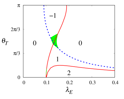
(a)

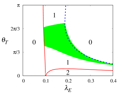
(b)

Figure 1: Phase diagrams of the proximity-modified graphene with twisted exchange couplings of strength $\lambda_{E}$ and twist angle $\theta_{T}$ for $\Delta=0.1$, $\lambda_{R}=0.05$, and (a) $\lambda_{I}=-0.05$; (b) $\lambda_{I}=0.05$. Red solid and blue dashed lines represent phase transition lines induced by band crossing near $K$ and $K^{\prime}$, respectively. The area marked in green denotes a metallic region. The numbers displayed indicate the Chern numbers of the corresponding topological phases.

The topological phases are characterized by Chern number defined by

$$C=\frac{1}{2\pi}\sum_{n}\int_{\textrm{BZ}}d^{2}k\ \ \Omega_{n}(\bm{k}),$$ (9)

where the summation of $n$ runs over all the filled valence bands and $\Omega_{n}(\bm{k})$ is Berry curvature of the $n$th valence band at momentum $\bm{k}$, defined by

$$\Omega_{n}(\bm{k}){=}-2\sum_{n^{\prime}\neq n}\frac{\textrm{Im}\langle\psi_{n,\bm{k}}|\partial_{k_{x}}H_{\bm{k}}|\psi_{n^{\prime},\bm{k}}\rangle\langle\psi_{n^{\prime},\bm{k}}|\partial_{k_{y}}H_{\bm{k}}|\psi_{n,\bm{k}}\rangle}{(E_{n^{\prime},\bm{k}}-E_{n,\bm{k}})^{2}},$$ (10)

with the eigenenergy $E_{n,\bm{k}}$ and the eigenfunction $\psi_{n,\bm{k}}$. By the exact diagonalization method, we obtain the eigenvalues and eigenvectors of the Fourier transformed Hamiltonian $H_{\bm{k}}$. Numerical integration of Berry curvature is performed over the Brillouin zone, which yields the Chern number of the phase.

Phase diagrams are constructed by the resulting Chern numbers for various exchange coupling strengths $\lambda_{E}$ and twist angles $\theta_{T}$. In Fig. 1 we plot two phase diagrams for $\lambda_{I}=\pm 0.05$ as mentioned in the previous section. The two systems have common behaviors in the topological phase transitions in the limits of small and large $\lambda_{E}$. For small $\lambda_{E}$ the system generally displays zero Chern number. On the other hand, for large $\lambda_{E}$, the system exhibits $C=2$ in the presence of uniform exchange coupling ($\theta_{T}=0$). As $\theta_{T}$ increases, the system undergoes two successive topological transitions and Chern number reduces by one at each transition. Thus, for staggered exchange coupling $(\theta_{T}=\pi)$, the resulting phase is topologically trivial in both limits.

In the intermediate region of exchange coupling strength $\lambda_{E}$ the topological characters of the two systems with $\lambda_{I}=\pm 0.05$ are very different. The system with $\lambda_{I}=-0.05$ exhibits three successive transitions from $C=2$ with the increase of $\theta_{T}$ and accordingly we obtain $C=-1$ for $\theta_{T}=\pi$. For $\lambda_{I}=0.05$, in contrast, only a single topological transition occurs with increasing $\theta_{T}$ and the phase with $C=1$ persists up to $\theta_{T}=\pi$ without further transitions.

At phase boundaries where Chern number changes by one the lower conduction band and the upper valence band touches at one point $\bm{k}_{0}$. One can find that we find two phase boundaries where $\bm{k}_{0}$ is near $K$ point (displayed in red solid lines) and one with $\bm{k}_{0}$ being near $K^{\prime}$ (displayed in blue dashed lines). It is of interest to note that $\bm{k}_{0}$ is located exactly at the symmetric point ($K$) only on the left red solid line. On the other two phase boundaries, $\bm{k}_{0}$ changes with $\lambda_{E}$ although $\bm{k}_{0}$ is close to $K$ or $K^{\prime}$ in the region displayed in Fig. 1. We have obtained the precise positions of the phase boundaries by numerically identifying the value of $\lambda_{E}^{c}(\theta_{T})$ for which the conduction and the valence bands touch each other and constructed the phase diagram in Fig. 1.

The analysis of the variation of the phase boundaries with $\theta_{T}$ reveals the the origin of the different behavior in the intermediate regions of $\lambda_{E}$. As illustrated in Fig. 1, we have one red($K$) and one blue($K^{\prime}$) boundary lines which traverse the whole range of $\theta_{T}$ between the uniform and the staggered exchange couplings. For $\lambda_{I}=0.05$ both $\lambda_{E}^{c}(K)$ and $\lambda_{E}^{c}(K^{\prime})$ decreases with the increase of $\theta_{T}$ and do not cross each other. Thus the phase with $C=1$ for small $\theta_{T}$ extends continuously to $\theta_{T}=\pi$. For $\lambda_{I}=-0.05$, on the other hand, $\lambda_{E}^{c}(K)$ increases with $\theta_{T}$ and the resulting phase boundary crosses the $K^{\prime}$ boundary line. The crossing point results in two more successive topological transitions and the system exhibits $C=-1$ at $\theta_{T}=\pi$

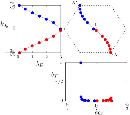
Figure 2: The band-touching momentum $\bm{k}_{0}$ of the proximity-modified graphene model with twisted exchange couplings on the phase boundaries as a function of $\lambda_{E}$ and $\theta_{T}$ for $\Delta=0.1$, $\lambda_{R}=0.05$, and $\lambda_{I}=-0.05$. A dashed hexagon indicates the boundary of the Brillouin zone and the crosses($\times$) indicate the location of symmetric points, $K$, $K^{\prime}$, and $\Gamma$ in the Brillouin zone.

Another interesting feature in the phase diagram is the existence of metallic regions for intermediate $\theta_{T}$. The metallic phase shows up when the minimum of the conduction band is lower than the maximum of the valence band, which yields partial filling in the conduction band without the overlap of valence and conduction bands. For $\lambda_{I}=-0.05$ the metallic region is located around the crossing point of two traversing $K$ and $K^{\prime}$ phase boundaries. Such a metallic region also appears for $\lambda_{I}=0.05$ in the middle of the region with $C=1$, and it separates $C=1$ phase for uniform exchange coupling from that for staggered exchange coupling.

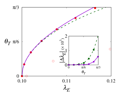
(a)

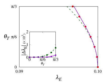
(b)

Figure 3: Comparison of phase boundaries from exact diagonalization and perturbative calculations in the proximity-modified graphene model with twisted exchange couplings for $\Delta=0.1$, $\lambda_{R}=0.05$ and (a) $\lambda_{I}=-0.05$; (b) $\lambda_{I}=0.05$. The phase boundaries estimated from exact diagonalization are marked by red circles, and green dashed and purple solid lines denote those obtained from the second-order and the fourth-order perturbation theory in the twist angle $\theta_{T}$, respectively. The insets show the absolute differences between the numerical and the perturbative values of $\lambda_{E}^{c}$ as a function of $\theta_{T}$.

Figure 2 displays how the band-touching momentum $\bm{k}_{0}$ changes as the system parameter varies. For small $\lambda_{E}$ two bands touch around $K$ point on the “red” boundary and around $K^{\prime}$ point on the “blue” boundary. As $\lambda_{E}$ increases, both $|k_{0x}|$ and $|k_{0y}|$ reduce and $\bm{k_{0}}$ monotonically approaches $\Gamma$ point. Although $K^{\prime}$ boundary line starts from $\theta_{T}=\pi$, we can find that the twist angle $\theta_{T}$ drastically decreases with the increase of $\lambda_{E}$. As demonstrated in Fig. 2 the band-touching momentum is close to $\Gamma$ for $\lambda_{E}\gtrsim 3$.

III.2 Perturbation Theory

In this section, we apply the perturbation theory to obtain the phase boundary which is determined by the band-touching at $K$ point. The characteristic equation of the Hamiltonian at $K$ is given by

$$\begin{split}\big{(}&\Delta-\lambda_{I}-\lambda_{E}-E\big{)}\times\\ \big{[}&\big{(}\Delta+\lambda_{I}+\lambda_{E}-E\big{)}\times\\ &\big{(}-\Delta-\lambda_{I}+\lambda_{E}\cos{\theta_{T}}-E\big{)}\times\\ &\big{(}-\Delta+\lambda_{I}-\lambda_{E}\cos{\theta_{T}}-E\big{)}\\ &-9\lambda_{R}^{2}\big{(}-\Delta-\lambda_{I}+\lambda_{E}\cos{\theta_{T}}-E\big{)}\\ &-\lambda_{E}^{2}\sin^{2}{\theta_{T}}\big{(}\Delta+\lambda_{I}+\lambda_{E}-E\big{)}\big{]}=0,\end{split}$$ (11)

where $E$ is an energy eigenvalue.

For $\theta_{T}=0$, four energy levels are given by

$$\begin{split}E_{1}^{(0)}=&\lambda_{I}-\sqrt{(\Delta+\lambda_{E})^{2}+9\lambda_{R}^{2}},\\ E_{2}^{(0)}=&-\lambda_{I}-\Delta+\lambda_{E},\\ E_{3}^{(0)}=&-\lambda_{I}+\Delta-\lambda_{E},\\ E_{4}^{(0)}=&\lambda_{I}+\sqrt{(\Delta+\lambda_{E})^{2}+9\lambda_{R}^{2}},\\ \end{split}$$ (12)

and the topological transition occurs at $\lambda_{E}=\Delta$ by the band-crossing of $E_{2}^{(0)}$ and $E_{3}^{(0)}$.

We apply the perturbation theory by trying the power-series solution of the energy eigenvalues

$$E_{i}=E_{i}^{(0)}+\sum_{n=1}^{\infty}c_{i}^{(n)}\theta_{T}^{n}\quad\quad(i=1,2,3,4).$$ (13)

Since the characteristic equation is an even function of $\theta_{T}$, $c_{i}^{(n)}=0$ for odd $n$. From the overall factor in Eq. (11) we can also find that $E_{3}=E_{3}^{(0)}$ is independent of $\theta_{T}$.

By inserting ${E_{2}}$ to Eq. (11) and expanding it to the fourth order in $\theta_{T}$, we find the first two nonvanishing coefficients

$$\begin{split}c_{2}^{(2)}=&-\frac{\lambda_{E}}{2}-\frac{2\lambda_{E}^{2}\big{(}\Delta+\lambda_{I}\big{)}}{4\big{(}\lambda_{I}-\lambda_{E}\big{)}\big{(}\Delta+\lambda_{I}\big{)}-9\lambda_{R}^{2}},\\ c_{2}^{(4)}=&\frac{\lambda_{E}}{24}+\frac{1}{4(\lambda_{I}-\lambda_{E})(\Delta+\lambda_{I})-9\lambda_{R}^{2}}\times\\ &\Big{[}\lambda_{E}^{2}(\Delta+\lambda_{I})/6+c_{2}^{(2)}\lambda_{E}\lambda_{I}\\ &\quad+2\left(c_{2}^{(2)}\right)^{2}(2\lambda_{I}-\lambda_{E}+\Delta)\Big{]}.\end{split}$$ (14)

Figure 3 displays the results from the perturbation calculation of the second and the fourth order in $\theta_{T}$ for $\lambda_{I}=\pm 0.05$. We can observe that second-order perturbation results reproduce the phase boundaries well at least up to $\theta_{T}=\pi/6$. The fourth-order results show better agreement for higher $\theta_{T}$ than the second-order ones. It is interesting that this approach identifies only one of two phase boundaries which split near $(\lambda_{E}=\Delta$ and $\theta_{T}=0)$. The reason is that the phase boundary denoted by open circles is caused by the band-touching which does not occur exactly at $K$ point. We will examine the peculiar features of this phase boundary in the next section.

III.3 Fine structures near the transition under uniform exchange coupling

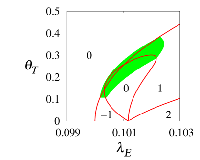
(a)

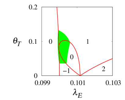
(b)

Figure 4: Phase diagram magnified in the vicinity of the transition point at $\theta_{T}=0$. The number displayed is the Chern number of the corresponding phase. The areas marked in green denote metallic regions.

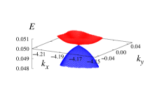
(a)

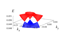
(b)

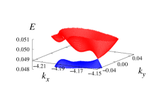
(c)

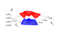
(d)

Figure 5: Energy dispersions of the proximity-modified graphene model with twisted exchange couplings for $\Delta=0.1$, $\lambda_{R}=0.05$, (a) $\lambda_{E}=0.1$, and $\theta_{T}=0$; (b) $\lambda_{E}=0.1012$, and $\theta_{T}=0$; (c) $\lambda_{E}=0.101655$, and $\theta_{T}=0.1775$; (d) $\lambda_{E}=0.10074$, and $\theta_{T}=0.04125$.

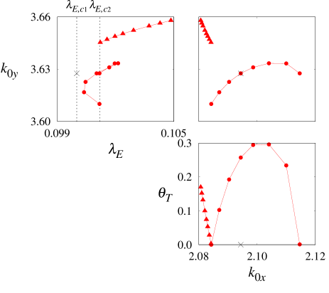
Figure 6: The band-touching momentum $\bm{k}_{0}$ of the proximity-modified graphene model with twisted exchange couplings on the phase boundaries as a function of $\lambda_{E}$ and $\theta_{T}$ for $\Delta=0.1$, $\lambda_{R}=0.05$, and $\lambda_{I}=-0.05$. The dotted lines are the two transition points $\lambda_{E,c1}$ and $\lambda_{E,c2}$ at $\theta_{T}=0$, and the cross($\times$) indicates $K$ point.

Figure 4 presents the phase diagram magnified in the vicinity of the topological transition at $\theta_{T}=0$. It is remarkable that for the uniform exchange coupling ($\theta_{T}=0$) the system does not exhibit a direct transition from a topologically trivial phase ($C=0$) for small $\lambda_{E}$ to a topological phase ($C=2$) for large $\lambda_{E}$. As $\lambda_{E}$ increases, the system undergoes a transition to a topological phase with $C=-1$ at $\lambda_{E,c1}=0.1$, and successively to a second topological phase with $C=2$ at $\lambda_{E,c2}=0.1012(1)$.

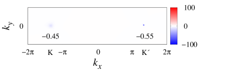
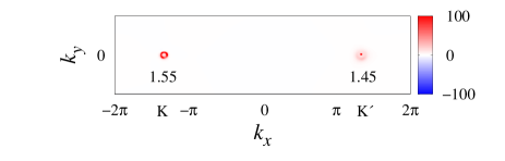
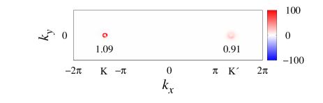
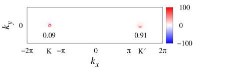
Figure 7: The distribution of Berry curvature in a Brillouin zone in the systems of $\theta_{T}=0.25$(left) and $\theta_{T}=0.7$(right). The range of the Brillouin zone is $-2\pi<k_{x}<2\pi$ and $-\frac{1}{\sqrt{3}}<k_{y}<\frac{1}{\sqrt{3}}$. The color on the momentum plane denotes Berry curvature ranging from -100 to 100. The numbers written in the plane are Chern numbers to which the Berry curvature is integrated over the half of the Brillouin zone including $K$ and $K^{\prime}$, respectively. The first, second, and third rows correspond to the lower valence band, the upper band valence band, and all the filled bands, respectively.

The energy dispersions at the transition points, plotted in Fig. 5(a) and (b), reveals the nature of two transitions. At $\lambda_{E,c1}=\Delta$, the valence and the conduction band touches at $K$ point and the Chern number decreases by one. In contrast, at $\lambda_{E,c2}$ the energy dispersion exhibits three band-touching points placed in the form of an equilateral triangle around $K$ point, which increases the Chern number by three. It is reminiscent of trigonal-warping deformation which is known to be induced in graphene by Rashba spin-orbit interaction Rakyta et al. (2010). The introduction of the sublattice potential shifts the topological transition point from $\lambda_{E}=0$ to $\lambda_{E,c1}=\Delta$, and we presume that it gives rise to additional fine splitting of the trigonal-warping deformation at $\lambda_{E,c2}$ from the $K$-point band-touching at $\lambda_{E,c1}$.

For finite $\theta_{T}$, each of three band-touching points produces different phase boundary lines, as shown in Fig. 4. Two of them merge at finite $\theta_{T}$, forming a closed phase boundary line which encloses a trivial phase with $C=0$. Two typical energy dispersions on the closed phase boundary line are shown in Figs. 5 (c) and (d). They show a single band-touching point with a distorted trigonal-warping deformation. The phase boundary line generated by the third band-touching point is that separating $C=2$ phase from $C=1$ phase; this is the one shown in the global phase diagram of Fig. 1. We can also observe that metallic regions emerge around the region where the closed phase boundary line is overlapped with that generated by the $K$-point band-touching for both systems.

We also display the band-touching momentum $\bm{k}_{0}$ on these phase boundaries in Fig. 6. As is discussed in the above, the three points at $\lambda_{E,c2}$ form an equilateral triangle, and two of them merge when $\theta_{T}$ is increased up to a critical value. The third band-touching point goes towards $\Gamma$ point as $\lambda_{E}$ is increased, and reaches close to $\Gamma$ point for very large $\lambda_{E}$.

III.4 Berry curvatures and winding numbers

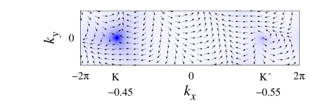
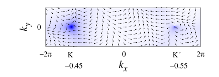
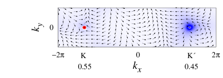
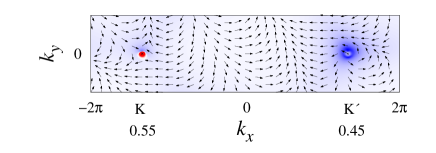
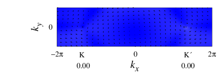
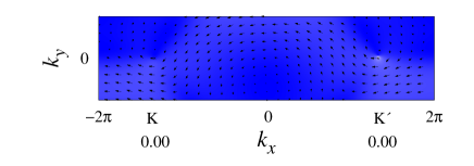
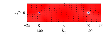
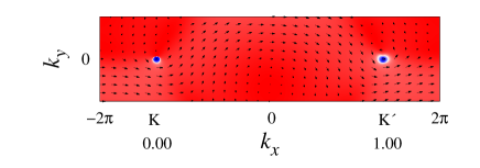
Figure 8: Spin textures of pseudo and real spins for both valence bands in the cases of $\theta_{T}=0.25$(left) and $\theta_{T}=0.7$(right). The upper(lower) two rows correspond to pseudo(real) spin textures. The first and the third rows correspond to the lower valence band and the second and the fourth rows to the upper valence band. Arrows on the Brillouin zone represent the planar components of pseudo or real spins and the color denotes those values of the $z$-component: blue$(-)$, white$(0)$, and red$(+)$. The numbers written below $K$ or $K^{\prime}$ are the contribution to the winding number from the half of the Brillouin zones around the point.

In this section, we demonstrate topological properties of the nontrivial phases in terms of Berry curvature and winding numbers. We focus on two systems with $\theta_{T}=0.25$ and $\theta_{T}=0.7$ for $\lambda_{I}=-0.05$ and $\lambda_{E}=0.15$. The former and the latter systems exhibit the topological phases with $C=2$ and $C=1$, respectively, as shown in Fig. 1(a).

Figure 7 shows the distribution of Berry curvature of the individual and all the valence bands. In both valence bands, Berry curvature concentrates on $K$ and $K^{\prime}$. In the case of $\theta_{T}=0.25$, the Berry curvature in the lower valence band contributes to the total Chern number negatively both in $K$ and $K^{\prime}$. However, those in the upper valence band are positive, which are much larger than those in the lower valence band. As a result, both $K$ and $K^{\prime}$ have positive Berry curvature peaks and their sum produces Chern number two. In the case of $\theta_{T}=0.7$, the Berry curvature distributions are more or less the same as in the case of $\theta_{T}=0.25$ except for the area around $K$. An additional negative peak shows up as well as a positive peak near $K$ in the upper valence band, and the Chern number of this area is reduced by one. Consequently, the total Chern number for $K$ is less than that of $\theta_{T}=0.25$ by one. Thus, the phase transition from $C=2$ to $C=1$ is attributed to the change of Berry curvature distribution around $K$ in the upper valence band.

The topological properties can also be represented in terms of the winding numbers in spin textures Qiao et al. (2012); Fradkin (2013); Bernevig and Hughes (2013); Fösel et al. (2017); Ren et al. (2016); Nagaosa and Tokura (2013); Yu et al. (2010). We calculate pseudo spin $\langle\bm{S}\rangle$ associated with two valleys and real spin $\langle\bm{\sigma}\rangle$ in momentum space and the winding number $\omega$ in each texture is defined by

$$\omega=-\frac{1}{4\pi}\int_{\rm BZ}\hat{\bm{M}}(\bm{k})\cdot\Big{(}\partial_{k_{x}}\hat{\bm{M}}(\bm{k})\times\partial_{k_{y}}\hat{\bm{M}}(\bm{k})\Big{)}d^{2}k,$$ (15)

where $\hat{\bm{M}}(\bm{k})$ is the unit vector in the direction of each spin at momentum $\bm{k}$. Chern number of the individual band is equal to the winding number, $C=\omega$ Fradkin (2013).

Figure 8 describes the pseudo and real spin textures in both valence bands. In the case of $\theta_{T}=0.25$, merons and antimerons in pseudo spin textures of lower and upper valence band cancel each other in both $K$ and $K^{\prime}$ while two skyrmions remain in both $K$ and $K^{\prime}$ in the real spin texture of upper valence band. Thus, the nontrivial property of the system comes from real spins in upper valence bands. As $\theta_{T}$ increases up to 0.7, the winding number changes from 1 to 0 due to the contribution in the vicinity of $K$ in the upper valence band. This is due to the destruction of a skyrmion at $K$ by the band-touching of the upper valence and the lower conduction bands at $K$.

IV Summary

In summary, we have investigate the topological phase transition of the modified graphene model under the twisted exchange couplings. By the variation of the twist in the directions of two sublattice exchange couplings we have successfully examined the nature of transitions between the topological phases under uniform exchange couplings and those under staggered exchange couplings. The resulting phase diagrams have been found to exhibit rich phases. We have performed the perturbative calculation in the twist angle, which was successful in describing the phase transition line near the uniform exchange couplings. Topological objects in real and pseudo spin textures have been shown to the source for the contribution to topological invariants of the system.

Remarkably, we have discovered that the transition from a trivial phase to a topological phase with Chern number two in uniform exchange coupling is not a direct transition. As the exchange coupling increases, the system first make a transition from the trivial phase to a topological phase with Chern number reduced by one. At a higher value of exchange coupling, the trigonal-warping deformation has been found to drive the system to the topological phase with Chern number two. The two close but separate transitions may have its origin in the interplay by the Rashba spin-orbit coupling and the staggered sublattice potential.

References

- Chang et al. (2023) C.-Z. Chang, C.-X. Liu, and A. H. MacDonald, Rev. Mod. Phys. 95, 011002 (2023).
- Liu et al. (2016) C.-X. Liu, S.-C. Zhang, and X.-L. Qi, Annu. Rev. Condens. Matter Phys. 7, 301 (2016).
- Liu et al. (2008) C.-X. Liu, X.-L. Qi, X. Dai, Z. Fang, and S.-C. Zhang, Phys. Rev. Lett. 101, 146802 (2008).
- Onoda and Nagaosa (2003) M. Onoda and N. Nagaosa, Phys. Rev. Lett. 90, 206601 (2003).
- Wu (2008) C. Wu, Phys. Rev. Lett. 101, 186807 (2008).
- von Klitzing et al. (1980) K. von Klitzing, G. Dorda, and M. Pepper, Phys. Rev. Lett. 45, 494 (1980).
- Thouless et al. (1982) D. J. Thouless, M. Kohmoto, M. P. Nightingale, and M. den Nijs, Phys. Rev. Lett. 49, 405 (1982).
- Qiao et al. (2010) Z. Qiao, S. A. Yang, W. Feng, W.-K. Tse, J. Ding, Y. Yao, J. Wang, and Q. Niu, Phys. Rev. B 82, 161414 (2010).
- Sheng et al. (2006) D. N. Sheng, Z. Y. Weng, L. Sheng, and F. D. M. Haldane, Phys. Rev. Lett. 97, 036808 (2006).
- Qiao et al. (2011) Z. Qiao, W.-K. Tse, H. Jiang, Y. Yao, and Q. Niu, Phys. Rev. Lett. 107, 256801 (2011).
- Bernevig and Hughes (2013) B. A. Bernevig and T. L. Hughes, Topological Insulators and Topological Superconductors (Princeton University Press, New Jersey, 2013).
- Fradkin (2013) E. Fradkin, Field Theories of Condensed Matter Physics (Cambridge University Press, Cambridge, 2013).
- Vanderbilt (2018) D. Vanderbilt, Berry Phases in Electronic Structure Theory (Cambridge University Press, Cambridge, 2018).
- Chang et al. (2013) C.-Z. Chang, J. Zhang, X. Feng, J. Shen, Z. Zhang, M. Guo, K. Li, Y. Ou, P. Wei, L.-L. Wang, Z.-Q. Ji, Y. Feng, S. Ji, X. Chen, J. Jia, X. Dai, Z. Fang, S.-C. Zhang, K. He, Y. Wang, L. Lu, X.-C. Ma, and Q.-K. Xue, Science 340, 167 (2013).
- Deng et al. (2020) Y. Deng, Y. Yu, M. Z. Shi, Z. Guo, Z. Xu, J. Wang, X. H. Chen, and Y. Zhang, Science 367, 895 (2020).
- Serlin et al. (2020) M. Serlin, C. L. Tschirhart, H. Polshyn, Y. Zhang, J. Zhu, K. Watanabe, T. Taniguchi, L. Balents, and A. F. Young, Science 367, 900 (2020).
- Haldane (1988) F. D. M. Haldane, Phys. Rev. Lett. 61, 2015 (1988).
- Kane and Mele (2005) C. L. Kane and E. J. Mele, Phys. Rev. Lett. 95, 226801 (2005).
- Qiao et al. (2012) Z. Qiao, H. Jiang, X. Li, Y. Yao, and Q. Niu, Phys. Rev. B 85, 115439 (2012).
- Bampoulis et al. (2023) P. Bampoulis, C. Castenmiller, D. J. Klaassen, J. van Mil, Y. Liu, C.-C. Liu, Y. Yao, M. Ezawa, A. N. Rudenko, and H. J. W. Zandvliet, Phys. Rev. Lett. 130, 196401 (2023).
- Högl et al. (2020) P. Högl, T. Frank, K. Zollner, D. Kochan, M. Gmitra, and J. Fabian, Phys. Rev. Lett. 124, 136403 (2020).
- Rakyta et al. (2010) P. Rakyta, A. Kormányos, and J. Cserti, Phys. Rev. B 82, 113405 (2010).
- Fösel et al. (2017) T. Fösel, V. Peano, and F. Marquardt, New J. Phys. 19, 115013 (2017).
- Ren et al. (2016) Y. Ren, Z. Qiao, and Q. Niu, Rep. Prog. Phys. 79, 066501 (2016).
- Nagaosa and Tokura (2013) N. Nagaosa and Y. Tokura, Nat. Nanotechnol. 8, 899 (2013).
- Yu et al. (2010) X. Z. Yu, Y. Onose, N. Kanazawa, J. H. Park, J. H. Han, Y. Matsui, N. Nagaosa, and Y. Tokura, Nature 465, 901 (2010).